Trapezoid central configurations

Abstract.

We classify all planar four–body central configurations where two pairs of the bodies are on parallel lines. Using Cartesian coordinates, we show that the set of four–body trapezoid central configurations with positive masses forms a two–dimensional surface where two symmetric families, the rhombus and isosceles trapezoid, are on its boundary. We also prove that, for a given position of the bodies, in some cases an specific order of the masses determine the geometry of the configuration, namely acute or obtuse trapezoid central configuration. We also prove the existence on non–symmetric trapezoid central configuration with two pairs of equal masses.

1. Introduction

Central configurations are particular positions of the masses in the Newtonian $n$–body problem, where the position and acceleration vectors with respect to the center of masses are proportional, with the same constant of proportionality for all masses. They play an important role in celestial mechanics because, among other properties, they generate the unique known explicit solutions in the $n$–body problem for $n\geq 3$. For general information about central configurations see for instance Albouy and Chenciner [4], Hagihara [22], Moeckel [33], Saari [38, 39], Schmidt [41], Smale [43, 44] and Wintner [47].

More precisely we consider the planar $n$–body problem

$$m_{k}\,\ddot{\mathbf{q}}_{k}=-\sum_{\scriptsize\begin{array}[]{c}j=1\\ j\neq k\end{array}}^{n}G\,m_{k}\,m_{j}\,\displaystyle{\frac{\mathbf{q}_{k}-\mathbf{q}_{j}}{|\mathbf{q}_{k}-\mathbf{q}_{j}|^{3}}}\ ,$$

$k=1,\dots,n$, being $\mathbf{q}_{k}\in\mathbb{R}^{2}$ the position vector of the punctual mass $m_{k}$ in an inertial coordinate system, and $G$ is the gravitational constant that we can take equal to one by choosing conveniently the unit of time. The configuration space of the planar $n$–body problem is

$$\mathcal{E}=\{(\mathbf{q}_{1},\dots,\mathbf{q}_{n})\in\mathbb{R}^{2n}\>:\>\mathbf{q}_{k}\neq\mathbf{q}_{j},\ \mbox{for }k\neq j\}.$$

A configuration of the $n$ bodies $(\mathbf{q}_{1},\dots,\mathbf{q}_{n})\in\mathcal{E}$ is central if there is a positive constant $\lambda$ such that

(1) $$\ddot{\mathbf{q}}_{k}=-\lambda\,\left(\mathbf{q}_{k}-\mathbf{c}\right)\ ,$$

for $k=1,\dots,n$, being $\mathbf{c}$ the position vector of the center of mass of the system, which is defined by $\mathbf{c}=\sum_{k=1}^{n}m_{k}\mathbf{q}_{k}/\sum_{k=1}^{n}m_{k}.$

Two planar central configurations are equivalent if there is a homothecy of $\mathbb{R}^{2}$ and a rotation of $SO(2)$ with respect to the center of mass which send one into the other. Since this relation is of equivalency, in what follows we shall consider the classes of equivalency of central configurations.

The complete set of planar central configurations of the $n$–body problem is only known for $n=2,3$. For $n=2$ there is only one class of central configurations. For each choice of three positive masses there are five classes of central configurations of the three–body problem, the three collinear central configurations found in 1767 by Euler [18], and the two equilateral triangle central configurations found in 1772 by Lagrange [25].

When $n>3$ there are many partial results for the number of classes of central configurations of the $n$–body problem. In 1910 Moulton [34] showed that there exists exactly $n!/2$ classes of collinear central configurations for any given set of positive masses, one for each ordering of the masses on the straight line modulo a rotation of $\pi$ radians. A lower bound of the number of planar non–collinear central configurations was obtained by Palmore in [35].

Although the set of all planar central configurations of the four–body problem is not completely known, we can find in the literature several papers that provide the existence and classification of central configurations of the four–body problem in some particular cases. For instance, a complete numerical study for the number of classes of central configurations for $n=4$ and arbitrary masses was done by Simó in [42]. A computer assisted proof of the finiteness of the number of central configurations for $n=4$ and any choice of the masses was given by Hampton and Moeckel [23]. Later on Albouy and Kaloshin [7] proved this result analytically, and extend it for for $n=5$, except for a zero measure set in the masses space .

Assuming that every central configuration of the four–body problem with equal masses has an axis of symmetry Llibre in [27] obtained all the planar central configurations of the four–body problem with equal masses by studying the intersection points of two planar curves. Later on Albouy in [1, 2] gave a complete analytic proof of this result.

When one of the four masses is sufficiently small Pedersen [36], Gannaway [20] and Arenstorf [10] numerically and analytically obtained the number of its classes of central configurations. These studies were completed later on by Barros and Leandro in [11] and [12].

A central configuration is called kite if it has an axis of symmetry passing through two non–adjacent bodies. The kite non–collinear classes of central configurations having some symmetry for the four–body problem with three equal masses where characterized by Bernat et al. in [13], see also Leandro [26]. The characterization of the convex central configurations with an axis of symmetry and the concave central configurations of the four–body problem when the masses satisfy that $m_{1}=m_{2}\neq m_{3}=m_{4}$ was done by Álvarez and Llibre in [9].

A planar configuration of the four–body problem can be classified as either convex or concave. A configuration is convex if none of the bodies is located in the interior of the triangle formed by the others. A configuration is concave if one of the bodies is in the interior of the triangle formed by the others.

In [31] MacMillan and Bartky shown that for any assigned order of any four positive masses there is a convex planar central configuration of the four–body problem with that order. Later on, Xia [49] provided a simpler proof of this result. The following convex conjecture stated by Albouy and Fu in [5] (see also [31, 37]) is well known between the community working in central configurations: For the planar four–body problem there is a unique convex central configuration of the four–body problem for each ordering of the masses in the boundary of its convex hull.

Already, MacMillan and Bartky in [31] proved that there exists a unique isosceles trapezoid central configuration of the four–body when two pairs of equal masses are located at adjacent vertices. Later on Xie in [50] reproved this result.

The following subconjecture of the convex conjecture is also well known: For the planar four–body problem there exists a unique convex central configuration having two pairs of equal masses located at the adjacent vertices of the configuration and it is an isosceles trapezoid.

In [29] Long and Sun shown that any convex central configuration with masses $m_{1}=m_{2}<m_{3}=m_{4}$ located at the opposite vertices of a quadrilateral and such that the diagonal corresponding to the mass $m_{1}$ is not shorter than the one corresponding to the mass $m_{3}$, has a symmetry and the quadrilateral is a rhombus. This result was extended by Pérez–Chavela [37] and Santoprete to the case where two of the masses are equal and at most, only one of the remaining mass is larger than the equal masses. Moreover, they proved that there is only one convex central configuration when the opposite masses are equal and it is a rhombus. Later on Albouy et. al. in [8] shown that in the four–body problem a convex central configuration is symmetric with respect to one diagonal if and only if the masses of the two particles on the other diagonal are equal. If these two masses are unequal, then the less massive one is closer to the former diagonal.

Using the results on the symmetries mentioned in the previous paragraph Corbera and Llibre [14] gave a complete description of the families of central configurations of the four–body problem with two pairs of equals masses and two equal masses sufficiently small, proving for these masses the convex conjecture and the subconjecture. More recently, the subconjecture was proved for arbitrary masses by Fernandes et al. in [19].

The co-circular classes of central configurations of the four–body problem, i.e. when the four masses are on a circle have been studied by Cors and Roberts in [15].

A trapezoid is a convex quadrilateral with at least one pair of parallel sides. The parallel sides are called the bases of the trapezoid and the other two sides are called the lateral sides. See Figure 1 for the classification of the nine trapezoids, namely:

• An acute trapezoid has two adjacent acute angles on its longer base edge.

• An obtuse trapezoid has one acute and one obtuse angle on each base.

• A right trapezoid has two adjacent right angles.

• An isosceles trapezoid is an acute trapezoid if its lateral sides have the same length, and the base angles have the same measure.

• A $3$–sides equal trapezoid is an isosceles trapezoid with three sides of the same length.

• A parallelogram is an obtuse trapezoid with two pairs of parallel sides.

• A rhombus is a parallelogram with the four sides with the same length.

• A rectangle is a parallelogram with four right angles.

• A square is a rectangle with the four sides with the same length.

Figure 1. Classification of Trapezoids

In this paper we are interested in studying trapezoid central configurations. See [40] for a really fresh work in the same topic. In section 3 we derive the equations for the trapezoid central configurations in terms of the mutual distances. In section 4 we prove that not all the trapezoid configurations are realizable. In section 5 we characterize, using cartesian coordinates, the set of positions that yield to trapezoid central configurations with positive masses. In section 6 we prove that there exist a one–parameter family of right trapezoid central configurations. Finally, in section 7 we study the set of positive masses which yields to a trapezoid central configurations. We prove, in contrast to the co–circular case, that two pair of equal masses do not imply that the central configuration has some symmetry.

2. Preliminaries

The central configurations (in what follows simply CC by short) can be described in terms of Lagrange multipliers. We denote by ${\bf q}=({\bf q}_{1},{\bf q}_{2},{\bf q}_{3},{\bf q}_{4})\in(\mathbb{R}^{2})^{4}$ the position of four positive masses $m_{1},m_{2},m_{3},m_{4}$ on the plane and by $r_{ij}=||\mathbf{q}_{i}-\mathbf{q}_{j}||$ the mutual distances between the $i$–th and the $j$–th bodies. The vector ${\bf q}$ is a CC of the $4$–body problem if it satisfies the following algebraic equation for some value of $\lambda$ (the Lagrange multiplier)

(2) $$\nabla U({\bf q})+\lambda\,\nabla I({\bf q})=0,$$

where $U$ is the Newtonian potential

(3) $$U({\bf q})=\sum_{i<j}^{n}\;\frac{m_{i}m_{j}}{r_{ij}},$$

$I({\bf q})$ is the moment of inertia, which represents the size of the system,

(4) $$I({\bf q})=\frac{1}{2}\sum_{i=1}^{n}m_{i}||\mathbf{q}_{i}-\mathbf{c}||^{2}=\frac{1}{2M}\sum_{1\leq i<j\leq n}\;m_{i}m_{j}r_{ij}^{2},$$

${\bf c}$ is the center of mass of the system, and $M=m_{1}+\cdots+m_{n}$ is the total mass (see [32] for more details).

We observe that generically six mutual distances describe a tetrahedron in $\mathbb{R}^{3}$, since in this work we are interested in planar CC, when we write equation (2) in terms of mutual distances, we must add a constraint to maintain the particles on a plane. This constraint arises setting the volume of the tetrahedron equals to zero. Denoting as ${\bf r}=(r_{12},r_{13},r_{14},r_{23},r_{24},r_{34})\in\mathbb{R}^{+^{6}}$ the vector of mutual distances, it is well know in the literature (see for instance [39, 41]), that the volume $V$ of a tetrahedron is given by the Cayley-Menger determinant

$$V^{2}\;=\;\frac{1}{288}\left|\begin{array}[]{ccccc}0&1&1&1&1\\ 1&0&r_{12}^{2}&r_{13}^{2}&r_{14}^{2}\\ 1&r_{12}^{2}&0&r_{23}^{2}&r_{24}^{2}\\ 1&r_{13}^{2}&r_{23}^{2}&0&r_{34}^{2}\\ 1&r_{14}^{2}&r_{24}^{2}&r_{34}^{2}&0\end{array}\right|.$$

From now on we will assume that $V=0$. Also in order to avoid collinear configurations we impose that all triples of mutual distances satisfy strictly the triangle inequality (see [15] for more details).

Let $A_{i}$ be the oriented area of the triangle formed by the configuration ${\bf q}$ where the point ${\bf q}_{i}$ is deleted, and let $\Delta_{i}=(-1)^{i+1}A_{i}$. Since $A_{i}>0$ when the vertices are ordered sequentially counterclockwise, for a convex quadrilateral ordered sequentially counterclockwise we obtain $\Delta_{1},\Delta_{3}>0$ and $\Delta_{2},\Delta_{4}<0,$ satisfying the equation

$$\Delta_{1}+\Delta_{2}+\Delta_{3}+\Delta_{4}=0.$$

In 1900 Dziobeck [17] proved for planar CC that

$$\frac{\partial V}{\partial r_{ij}^{2}}\;=\;-32\,\Delta_{i}\Delta_{j}\,.$$

From this equality we obtain

$$\frac{\partial V}{\partial r_{ij}}=\frac{\partial V}{\partial r_{ij}^{2}}\cdot\frac{d(r_{ij}^{2})}{dr_{ij}}=-64r_{ij}\,\Delta_{i}\Delta_{j}.$$

Fixing the moment of inertia $I=I_{0}$ and applying Lagrange multipliers, we have that the planar non-collinear CC are the critical points of the function

(5) $$U+\lambda M(I-I_{0})-\sigma V.$$

Taking the partial derivatives and using the six mutual distances as variables we obtain

$$m_{1}m_{2}(r_{12}^{-3}-\lambda)=64\sigma\Delta_{1}\Delta_{2}, m_{3}m_{4}(r_{34}^{-3}-\lambda)=64\sigma\Delta_{3}\Delta_{4},$$

(6) $$m_{1}m_{3}(r_{13}^{-3}-\lambda)=64\sigma\Delta_{1}\Delta_{3}, m_{2}m_{4}(r_{24}^{-3}-\lambda)=64\sigma\Delta_{2}\Delta_{4},$$

$$m_{1}m_{4}(r_{14}^{-3}-\lambda)=64\sigma\Delta_{1}\Delta_{4}, m_{2}m_{3}(r_{23}^{-3}-\lambda)=64\sigma\Delta_{2}\Delta_{3}.$$

Grouping the above equations by row, so that the product of the right-hand side is simply $(64\sigma)^{2}\Delta_{1}\Delta_{2}\Delta_{3}\Delta_{4}$, and since the masses are positive we obtain the well known Dziobeck relation

(7) $$(r_{12}^{-3}-\lambda)(r_{34}^{-3}-\lambda)=(r_{13}^{-3}-\lambda)(r_{24}^{-3}-\lambda)=(r_{14}^{-3}-\lambda)(r_{23}^{-3}-\lambda),$$

which must be satisfied for any planar 4-body CC. Solving each of the three pairs of equations for $\lambda$ we obtain

(8) $$\begin{array}[]{rl}\lambda\;=&\dfrac{r_{12}^{-3}\,r_{34}^{-3}-r_{13}^{-3}\,r_{24}^{-3}}{r_{12}^{-3}+r_{34}^{-3}-r_{13}^{-3}-r_{24}^{-3}}\\ =&\dfrac{r_{13}^{-3}\,r_{24}^{-3}-r_{14}^{-3}\,r_{23}^{-3}}{r_{13}^{-3}+r_{24}^{-3}-r_{14}^{-3}-r_{23}^{-3}}\\ =&\dfrac{r_{14}^{-3}\,r_{23}^{-3}-r_{12}^{-3}\,r_{34}^{-3}}{r_{14}^{-3}+r_{23}^{-3}-r_{12}^{-3}-r_{34}^{-3}}.\end{array}$$

If we set

$$\begin{array}[]{ccc}s_{1}=r_{12}^{-3}+r_{34}^{-3},&&p_{1}=r_{12}^{-3}r_{34}^{-3},\\[5.05942pt] s_{2}=r_{13}^{-3}+r_{24}^{-3},&&p_{2}=r_{13}^{-3}r_{24}^{-3},\\[5.05942pt] s_{3}=r_{14}^{-3}+r_{23}^{-3},&&p_{3}=r_{14}^{-3}r_{23}^{-3},\end{array}$$

then equation (8) can be written as

(9) $$\lambda\;=\;\frac{p_{1}-p_{2}}{s_{1}-s_{2}}\;=\;\frac{p_{2}-p_{3}}{s_{2}-s_{3}}\;=\;\frac{p_{3}-p_{1}}{s_{3}-s_{1}},$$

which means that $(s_{1},p_{1}),(s_{2},p_{2}),(s_{3},p_{3})$, viewed as points in $\mathbb{R}^{+2}$, must lie on the same line with slope $\lambda$. This in turn, is equivalent to

$$\left|\begin{array}[]{ccc}1&1&1\\[3.61371pt] s_{1}&s_{2}&s_{3}\\[3.61371pt] p_{1}&p_{2}&p_{3}\end{array}\right|\;=\;0,$$

a representation that allows to write Dziobeck equation (7) as the nice factorization

$$D=(r_{13}^{3}-r_{12}^{3})(r_{23}^{3}-r_{34}^{3})(r_{24}^{3}-r_{14}^{3})-(r_{12}^{3}-r_{14}^{3})(r_{24}^{3}-r_{34}^{3})(r_{13}^{3}-r_{23}^{3})=0$$

The Dziobeck equation $D=0$ must be satisfied for the six mutual distances of every four-body planar central configuration.

3. Equations of trapezoidal central configurations

We consider four positive masses $m_{1},m_{2},m_{3},m_{4}$ located at the vertices of a trapezoid, i.e. located by pairs on two parallel lines, which without loss of generality we assume are vertical. Since the central configurations are invariant under homotheties we can take the distance between the two parallel lines equal to one, after normalizing the unity of mass we can assume that $m_{1}=1$ located at the bottom part of the left line, $m_{2}$ above $m_{1}$ on the same line and $m_{3}$ above $m_{4}$ on the right line (see Fig. 2). From now on we will use this ordering and normalization of the units of mass and length in this work.

Figure 2. Central configurations with two parallel lines

All trapezoidal central configurations are convex, so from the results of McMillan [31], we know first that the diagonals of the respective quadrilateral are longer that any of the four sides, that is

(10) $$r_{13},r_{24}\;>\;r_{12},r_{14},r_{23},r_{34};$$

and second that the bigger and the smaller sides of the quadrilateral correspond to opposite sides. We note that in the restricted problem, i.e. when one or more masses are equal to zero, one of the sides of the quadrilateral could be equal to one diagonal.

Lemma 1.

The biggest side of the quadrilateral is on the parallel lines.

Proof.

Assume that $r_{23}$ is the biggest side and that we exclude the case where all the sides are equal, that is, the square. So, its opposite side, $r_{14}$, has to be the smaller one, and

$$r_{13},r_{24}\;>\;r_{23}\;\geq\;r_{12},r_{34}\;\geq\;r_{14}>1.$$

Then depending on the relative position of the four masses we have the following four scenarios:

• $r_{34}=r_{12}+\sqrt{r_{23}^{2}-1}+\sqrt{r_{14}^{2}-1},$

• $r_{34}=r_{12}+\sqrt{r_{23}^{2}-1}-\sqrt{r_{14}^{2}-1},$

• $r_{34}=r_{12}-\sqrt{r_{23}^{2}-1}+\sqrt{r_{14}^{2}-1},$

• $r_{34}=r_{12}-\sqrt{r_{23}^{2}-1}-\sqrt{r_{14}^{2}-1}.$

Notice that the cases where $m_{3}$ and $m_{4}$ are either both above $m_{2}$ or both below $m_{1}$ are not possible because in these cases one of the diagonals would be smaller than one of the sides.

In all scenarios we will arrive to a contradiction with the fact that $r_{23}$ is the biggest side or $r_{14}$ the smaller one.

In the scenario (a), $r_{34}>r_{12}+\sqrt{r_{23}^{2}-1}>1+\sqrt{r_{23}^{2}-1}>r_{23}$.

For the scenarios (b) and (c) we shall use the following result: Let $x,y\geq 1$ be two real numbers,

$$x-\sqrt{x^{2}-1}+\sqrt{y^{2}-1}=y\quad\text{if and only if}\quad x=y.$$

Moreover if $y>x$ then $x-\sqrt{x^{2}-1}+\sqrt{y^{2}-1}>y$, and if $y<x$ then $x-\sqrt{x^{2}-1}+\sqrt{y^{2}-1}<y$.

In (b) $r_{34}>\sqrt{r_{23}^{2}-1}+r_{14}-\sqrt{r_{14}^{2}-1}>r_{23}$, and in (c) $r_{34}<r_{23}-\sqrt{r_{23}^{2}-1}+\sqrt{r_{14}^{2}-1}<r_{14}$.

Finally, in (d) $r_{34}<r_{23}-\sqrt{r_{23}^{2}-1}+\sqrt{r_{14}^{2}-1}<r_{14}$ from scenario (c).

Similar argument works if $r_{14}>1$ is considered the biggest side. ∎

Without loss of generality we label the bodies so that $r_{12}$ is the longest side. We can also assume that $r_{23}\geq r_{14}$ by an appropriate relabeling. Indeed, equations (2) are invariant if we interchange bodies $m_{1}$ and $m_{2}$ and bodies $m_{3}$ and $m_{4}$. The choice $r_{23}\geq r_{14}$, together with the fact that $r_{12}$ is the longest side, implies the relation $r_{24}\geq r_{13}$ between the two diagonals.

Summarizing, we have proved the following result.

Lemma 2.

Labelling conveniently the bodies, the mutual distances that can provide trapezoid central configurations can be restricted to the following set

$$\widetilde{\Omega}=\{{\mathbb{r}}\in\mathbb{{R}^{+}}^{6}:r_{24}\geq r_{13}>r_{12}\geq r_{23}\geq r_{14}\geq r_{34}\}.$$

Next we give the expression of the masses ratios for the trapezoid central configurations on $\widetilde{\Omega}$. Taking into account the sign of the areas $A_{i}$, we have $\Delta_{1}=-r_{34}/2,\,\Delta_{2}=r_{34}/2,\,\Delta_{3}=-r_{12}/2,\,\Delta_{4}=r_{12}/2$ (note that we have considered the bodies ordered clockwise). Now from (2) we obtain the following ratios of the masses

(11) $$\frac{m_{2}}{m_{1}} = \frac{(\lambda-r_{13}^{-3})}{(r_{23}^{-3}-\lambda)}\;=\;\frac{(\lambda-r_{14}^{-3})}{(r_{24}^{-3}-\lambda)},$$

(12) $$\frac{m_{3}}{m_{1}} = \frac{(r_{12}^{-3}-\lambda)\,r_{12}}{(r_{23}^{-3}-\lambda)\,r_{34}}\;=\;\frac{(r_{14}^{-3}-\lambda)\,r_{12}}{(r_{34}^{-3}-\lambda)\,r_{34}},$$

(13) $$\frac{m_{4}}{m_{1}} = \frac{(r_{12}^{-3}-\lambda)\,r_{12}}{(\lambda-r_{24}^{-3})\,r_{34}}\;=\;\frac{(\lambda-r_{13}^{-3})\,r_{12}}{(r_{34}^{-3}-\lambda)\,r_{34}}.$$

We observe that the fact that all masses must be positive places additional constraints on the mutual distances. Using $\lambda=(p_{2}-p_{3})/(s_{2}-s_{3})$ and $m_{1}=1$ into the first equation in (11) and after some simplifications we obtain

(14) $$m_{2}=\frac{r_{23}^{3}r_{24}^{3}\,(r_{13}^{3}-r_{14}^{3})}{r_{13}^{3}r_{14}^{3}\,(r_{24}^{3}-r_{23}^{3})}.$$

Doing similar substitutions in (12) and (13) we get

(15) $$m_{3}=\frac{r_{23}^{3}r_{34}^{2}\,(r_{12}^{3}-r_{14}^{3})}{r_{12}^{2}r_{14}^{3}\,(r_{23}^{3}-r_{34}^{3})},$$

and

(16) $$m_{4}=\frac{r_{24}^{3}r_{34}^{2}\,(r_{13}^{3}-r_{12}^{3})}{r_{12}^{2}r_{13}^{3}\,(r_{24}^{3}-r_{34}^{3})},$$

respectively.

The masses of equations (14), (15) and (16) are positive and well-defined on $\widetilde{\Omega}$, except when $r_{12}=r_{14}$ and $r_{23}=r_{34}$ simultaneously. In that case, we use $\lambda=(p_{1}-p_{2})/(s_{1}-s_{2})$ into equation (12) getting

(17) $$m_{3}\;=\;\frac{r_{34}^{5}(r_{14}^{3}-r_{24}^{3})(r_{14}^{3}-r_{13}^{3})}{r_{14}^{5}(r_{13}^{3}-r_{34}^{3})(r_{24}^{3}-r_{34}^{3})},$$

which also is positive and well-defined on $\widetilde{\Omega}$.

In summary we have proved the next result.

Lemma 3.

Let

$$\widetilde{\Omega}^{\prime}=\{{\mathbb{r}}\in\mathbb{{R}^{+}}^{6}\ :{\mathbb{r}}\in\widetilde{\Omega}\,\,and\,\,D=0\}.$$

Any point in $\widetilde{\Omega}^{\prime}$ defines a four–body trapezoid central configuration with positive masses. Moreover, up to relabelling and rescaling the set $\widetilde{\Omega}^{\prime}$ contains all trapezoid central configurations.

4. The trapezoids which are not realizable as central configuration

In this section we prove that the vertices of the parallelogram, the rectangle and the $3$–sides equal trapezoid are not realizable as central configurations of the four-body problem with the exception of the square and the rhombus.

Assume that the bodies are ordered sequentially as in Figure 2.

Proposition 4.

In the planar four–body problem there are no parallelogram shape central configurations with positive masses at their vertices, excluding squares and rhombus.

Proof.

In a parallelogram configuration $r_{12}=r_{34}$ and $r_{23}=r_{14}$. From Lemma 3, this parallelogram could be realizable as a central configuration if $r_{12}=r_{23}=r_{14}=r_{34}$, that is, if it is a rhombus or a square. ∎

The next result is an immediate consequence of Proposition 4.

Corollary 5.

In the planar four–body problem there are no rectangle shape central configurations with positive masses at their vertices.

Proposition 6.

In the planar four–body problem there are no $3$–sides equal trapezoid shape central configurations with positive masses at their vertices, excluding the square.

Proof.

A $3$–sides equal trapezoid is in particular an isosceles trapezoid, so the length of its diagonals are equal. Assume that $r_{12}$ is the longest exterior side, that the equal sides are $r_{23}=r_{14}=r_{34}=\alpha<r_{12}$ and that the diagonals are $r_{24}=r_{13}=\beta$. Then from de Dziobeck equation $D=0$ we get

$$\left(\beta^{3}-\alpha^{3}\right)^{2}\left(\alpha^{3}-r_{12}^{3}\right)=0.$$

So either $r_{12}=r_{23}=r_{14}=r_{34}=\alpha$ and $r_{24}=r_{13}=\beta$ which corresponds to a square, or $\beta=\alpha$ which is not possible because it implies $r_{24}=r_{13}=r_{12}=r_{23}=r_{14}=r_{34}=\alpha$ (see Lemma 3).

Proceeding in a similar way when the equal sides are $r_{12}=r_{23}=r_{14}=\alpha>r_{34}$ the Dziobeck equation becomes

$$\left(\beta^{3}-\alpha^{3}\right)^{2}\left(\alpha^{3}-r_{34}^{3}\right)=0.$$

When $r_{34}=\alpha$ we get again the square and when $\beta=\alpha$ we get condition $r_{24}=r_{13}=r_{12}=r_{23}=r_{14}>r_{34}$. This condition can be satisfied only when the positions of $m_{3}$ and $m_{4}$ coincide and the resulting configuration is an equilateral triangle. Substituting the above relation into (15) and (16) we get $m_{3}=m_{4}=0$. ∎

5. The set of realizable trapezoid central configurations

In this section we characterize the set of realizable trapezoid central configurations.

Proposition 7.

The boundaries of $\widetilde{\Omega}^{\prime}$ (see Lemma 3) consist of a square, a curve corresponding to the rhombus, a curve containing the isosceles trapezoids and a curve corresponding to degenerate central configurations with $m_{4}=0$.

Proof.

The possible boundaries of $\widetilde{\Omega}^{\prime}$ are the sets where either $r_{24}=r_{13}$, $r_{13}=r_{12}$, $r_{12}=r_{23}$, $r_{23}=r_{14}$, or $r_{14}=r_{34}$. Next we characterize these boundaries.

Case A: $r_{24}=r_{13}$. The trapezoids having equal diagonals are the rectangle, the square and the isosceles trapezoid. The rectangle is not a realizable central configuration.

Case B: $r_{13}=r_{12}$. After substituting $r_{13}=r_{12}$ into equation $D=0$ we get the following three subcases. Note that the configurations coming from this condition are central configurations of the restricted problem; i.e. with one or more masses equal to zero.

• $r_{12}=r_{14}$. This implies $r_{12}=r_{23}=r_{14}$, so the masses $m_{1}$, $m_{2}$, $m_{3}$ and $m_{4}$ are located at the vertices of an equilateral triangle with $r_{34}=0$.

• $r_{12}=r_{23}$. In this case $r_{13}=r_{12}=r_{23}$, this means that the masses $m_{1}$, $m_{2}$, and $m_{3}$ are at the vertices of an equilateral triangle.

• $r_{24}=r_{34}$. This implies $r_{24}=r_{13}=r_{12}=r_{23}=r_{14}=r_{24}$ which is not possible.

Case C: $r_{12}=r_{23}$. After substituting $r_{12}=r_{23}$ into equation $D=0$ we get the following subcacases.

• $r_{13}=r_{23}$. Corresponds to case B.2.

• $r_{23}=r_{24}$. This implies $r_{24}=r_{13}=r_{12}=r_{23}$, so it corresponds also to case B.2.

• $r_{14}=r_{34}$. In this case $r_{12}=r_{23}$ and $r_{14}=r_{34}$, so the configuration is a kite. Since the configuration must be also a trapezoid it is necessarily a rhombus.

Case D: $r_{23}=r_{14}$. The trapezoids having two equal sides are the isosceles trapezoid, the rhombus, the square, the parallelogram and the rectangle. The last two do not correspond to realizable central configurations (see Proposition 6).

Case E: $r_{14}=r_{34}$. After substituting $r_{14}=r_{34}$ into equation $D=0$ we get the following subcacases.

• $r_{12}=r_{23}$. Corresponds to case C.3.

• $r_{13}=r_{34}$. This implies $r_{13}=r_{12}=r_{23}=r_{14}=r_{34}$, so the configuration is a rhombus.

• $r_{24}=r_{34}$. Corresponds to case B.3.

∎

Next we give the shape of the set of realizable trapezoid central configurations. To simplify the computations we parametrize the set of realizable central configurations by using the positions of the masses: $q_{1}=(0,0),q_{2}=(0,a),q_{3}=(1,b),q_{4}=(1,c)$, with $a\geq 1$ and $b>c$, and substituting the corresponding mutual distances into the Dziobeck equation $D=0$. This equation gives a relation between $a,b,c$ which provides an implicit $2$–dimensional surface in $\mathbb{R}^{3}$.

Theorem 8.

Let $q_{1}=(0,0),q_{2}=(0,a),q_{3}=(1,b),q_{4}=(1,c)$, with $a\geq 1$ and $b>c$, be the positions of the masses $m_{1}$, $m_{2}$, $m_{3}$ and $m_{4}$ respectively, then the set $\Omega$ of realizable CC is

$$\{(a,b,c)\in\mathbb{R}^{3}\ :\ a\geq 1,\ b>c,\ D=0,r_{24}\geq r_{13}>r_{12}\geq r_{23}\geq r_{14}\geq r_{34}\},$$

and the boundary of $\Omega$ is $\mathcal{C}_{1}\cup\mathcal{C}_{2}\cup\mathcal{C}_{3}\cup P_{1}\cup P_{2}\cup P_{3}$ where

$$\begin{split}\mathcal{C}_{1}&=\{(2/\sqrt{3},1/\sqrt{3},c)\>:\>c\in(-1/\sqrt{3},1/\sqrt{3})\},\\ \mathcal{C}_{2}&=\{\left(\sqrt{1+c^{2}},c+\sqrt{1+c^{2}},c\right)\>:\>c\in(-1/\sqrt{3},0)\},\\ \mathcal{C}_{3}&=\{(a,b,c)\ :\ a=b+c,f(b,c)=0,c\in(0,1/\sqrt{3})\},\\ P_{1}&=(2/\sqrt{3},1/\sqrt{3},1/\sqrt{3}),\\ P_{2}&=(2/\sqrt{3},1/\sqrt{3},-1/\sqrt{3}),\\ P_{3}&=(1,1,0),\end{split}$$

and

$$\begin{split}f(b,c)=&\left((b+c)^{3}-(c^{2}+1)^{3/2}\right)\left((b^{2}+1)^{3/2}-(b-c)^{3}\right)-\\ &\left((b^{2}+1)^{3/2}-(b+c)^{3}\right)\left((c^{2}+1)^{3/2}-(b-c)^{3}\right).\end{split}$$

See Figure 3 for the plot of the set $\Omega$.

The points of $\mathcal{C}_{1}$ provide configurations of the restricted problem with $m_{1}$, $m_{2}$ and $m_{3}$ in an equilateral triangle; the points of $\mathcal{C}_{2}$ and $\mathcal{C}_{3}$ provide rhombus and isosceles trapezoid central configurations, respectively; $P_{1}$ corresponds to an equilateral triangle configuration of the restricted problem with a collision of $m_{3}$ and $m_{4}$ at one of the vertices; $P_{2}$ corresponds to a configuration of the restricted problem with the masses at the vertices of a rhombus and such that the positions of $m_{1}$, $m_{2}$ and $m_{3}$ are the vertices of an equilateral triangle; and $P_{3}$ corresponds to the square central configuration.

Proof.

Easily we can compute $r_{24}=\sqrt{1+(a-c)^{2}}$, $r_{13}=\sqrt{1+b^{2}}$, $r_{12}=a$, $r_{23}=\sqrt{1+(a-b)^{2}}$, $r_{14}=\sqrt{1+c^{2}}$, and $r_{34}=b-c$. Proposition 7 gives the characterization of the central configurations on the boundaries of $\Omega$. We prove the result by using this characterization and the parametrization $(a,b,c)$.

On the boundary with the masses $m_{1}$, $m_{2}$ and $m_{3}$ at the vertices of an equilateral triangle we have $r_{13}=r_{12}=r_{23}$. Solving the system of equations $r_{13}=r_{12}=r_{23}$, we get $a=2/\sqrt{3}$ and $b=1/\sqrt{3}$. Substituting this solution into $r_{23}$ and $r_{14}$ and imposing the condition $r_{23}\geq r_{14}$, we get the condition $-1/\sqrt{3}\leq c\leq 1/\sqrt{3}$. It is easy to check that the solution $(a,b,c)=(2/\sqrt{3},1/\sqrt{3},c)$ with $c\in[-1/\sqrt{3},1/\sqrt{3}]$ satisfies $r_{24}\geq r_{13}\geq r_{12}\geq r_{23}\geq r_{14}\geq r_{34}$. So the set $\mathcal{C}_{1}\cup P_{1}\cup P_{2}$ belongs to the boundary of $\Omega$. Moreover it is easy to check that the point $P_{1}$ correspond to an equilateral triangle configuration with the masses $m_{3}$ and $m_{4}$ colliding at the corresponding vertex of the triangle; and the point $P_{2}$ corresponds to a rhombus configuration such that $m_{1}$, $m_{2}$ and $m_{3}$ are at the vertices of an equilateral triangle.

On the rhombus configurations we have $r_{12}=r_{23}=r_{14}=r_{24}$. Solving the system of equations $r_{12}=r_{23}=r_{14}=r_{24}$ we get the solution $s(c)=(a,b)=(\sqrt{1+c^{2}},c+\sqrt{1+c^{2}})$. Imposing that this solution satisfies $r_{24}\geq r_{13}>r_{12}$ we get the condition $-1/\sqrt{3}<c\leq 0$. So $\mathcal{C}_{2}$ belongs to the boundary of $\Omega$. Moreover $s(0)=(1,1)$ and $s(-1/\sqrt{3})=(2/\sqrt{3},1/\sqrt{3})$. So the endpoints of $\mathcal{C}_{2}$ are $P_{2}$ and $P_{3}$.

On the isosceles trapezoid, configurations $(a,b,c)$ are such that $r_{23}=r_{14}$, $r_{24}=r_{13}$ and $D=0$. If $r_{23}=r_{14}$ and $r_{24}=r_{13}$, then the Dziobeck equation $D=0$ becomes

$$\left(r_{14}^{3}-r_{13}^{3}\right)\left(\left(r_{12}^{3}-r_{14}^{3}\right)\left(r_{13}^{3}-r_{34}^{3}\right)-\left(r_{13}^{3}-r_{12}^{3}\right)\left(r_{14}^{3}-r_{34}^{3}\right)\right)=0.$$

If $r_{14}=r_{13}$, then $r_{24}=r_{13}=r_{12}=r_{23}=r_{14}$. This corresponds to the point $P_{1}$ (see the proof of Proposition 6). Assume now that $r_{14}\neq r_{13}$. Solving system $r_{23}=r_{14}$, $r_{24}=r_{13}$ we get $a=b+c$. So $r_{24}=r_{13}=\sqrt{b^{2}+1}$, $r_{12}=b+c$, $r_{23}=r_{14}=\sqrt{c^{2}+1}$, and $r_{34}=b-c$ and condition $D=0$ is equivalent to condition $f(b,c)=0$. Cors and Roberts in [15], using a different parametrization, proved the existence of a unique one-parameter family of isosceles trapezoid central configurations which is characterized by a differentiable function of one of the parameters in the parameter space. Moreover they prove that the endpoints of this family are the square configuration and the configuration consisting of an equilateral triangle with the masses $m_{3}=m_{4}=0$ at one of the vertices. In our parametrization the differentiable function of the parameter is the function $b(c)$ defined implicitly by $f(b,c)=0$ and the endpoints of the curve are the points $P_{1}$ and $P_{3}$. Thus $\mathcal{C}_{3}$ is the last curve in the boundary of $\Omega$ and it is a curve joining $P_{1}$ and $P_{3}$, see Figure 3. ∎

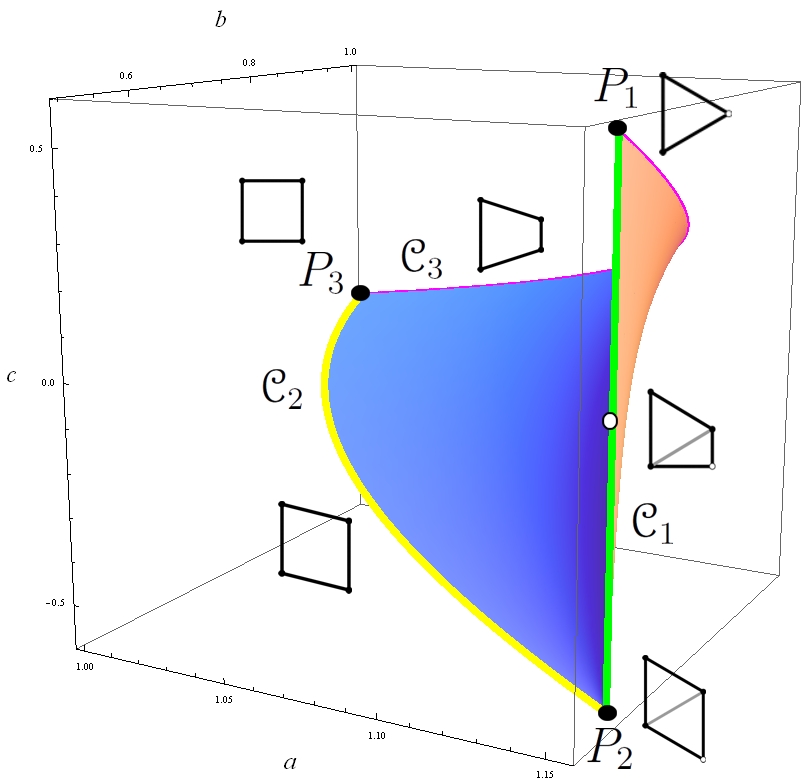
Figure 3. The surface $\Omega$ of the trapezoid central configurations in the $abc$–space.

Unfortunately we are not able to prove that $\Omega$ is a differentiable function over the two positions of the masses, as was stablish in the co–circular case, see [15]. Nevertheless, in the next section we prove that there exist a one–parameter family of trapezoid central configurations that divides $\Omega$ in two disjoint regions, namely the region that contains the trapezoid central configurations and the one that contains the obtuse trapezoid central configurations.

6. The right trapezoid family

We suppose again that we are in the hypotheses of Lemma 2; i.e. that $r_{12}\geqslant r_{23}\geqslant r_{14}\geqslant r_{34}$. We assume also that the position of the masses $m_{1}=1,m_{2},m_{3}$ and $m_{4}$ are respectively $(0,0),(0,a),(1,b),(1,0)$ with $a\geqslant 1$ and $a\geqslant b>0$. Easily we can compute the mutual distances $r_{12}=a,r_{23}=\sqrt{1+(a-b)^{2}},r_{14}=1,r_{34}=b,$ and $r_{13}=\sqrt{1+b^{2}}$ and $r_{24}=\sqrt{1+a^{2}}$ (the diagonals).

First we give the set $\widetilde{\Omega}$ (see Lemma 2) on the right trapezoid family parameterized by the positions of the masses $(a,b)$. It is obvious that condition $r_{24}>r_{12}$ is always satisfied and that condition $r_{34}\leqslant r_{14}$ implies $b\leqslant 1$. On the other hand, it is easy to see that conditions $r_{13}>r_{12}$ and $r_{12}\geqslant r_{23}$ imply that $a<a_{1}(b)=\sqrt{1+b^{2}}$ and $a\geqslant a_{2}(b)=(b^{2}+1)/(2b)$ respectively. From here we get condition $a_{1}(b)>a_{2}(b)$ which is satisfied for $b>1/\sqrt{3}$. In short, the set $\widetilde{\Omega}$ (see Lemma 2) on the right trapezoid family is

$$\Omega_{r}=\left\{(a,b,c)\in\mathbb{R}^{3}\>:\>\frac{b^{2}+1}{2b}\leqslant a<\sqrt{1+b^{2}},\quad\frac{1}{\sqrt{3}}<b\leqslant 1,\quad c=0\right\}.$$

We can see that $a_{1}$ is a decreasing function in $b\in(1/\sqrt{3},1]$ with $a_{1}(1/\sqrt{3})=2/\sqrt{3}$ and $a_{1}(1)=1$, whereas $a_{2}$ is an increasing function in $b\in(1/\sqrt{3},1]$ with $a_{2}(1/\sqrt{3})=2/\sqrt{3}$ and $a_{2}(1)=\sqrt{2}$ (see Figure 4). Therefore $a\in(1,\sqrt{2})$.

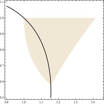
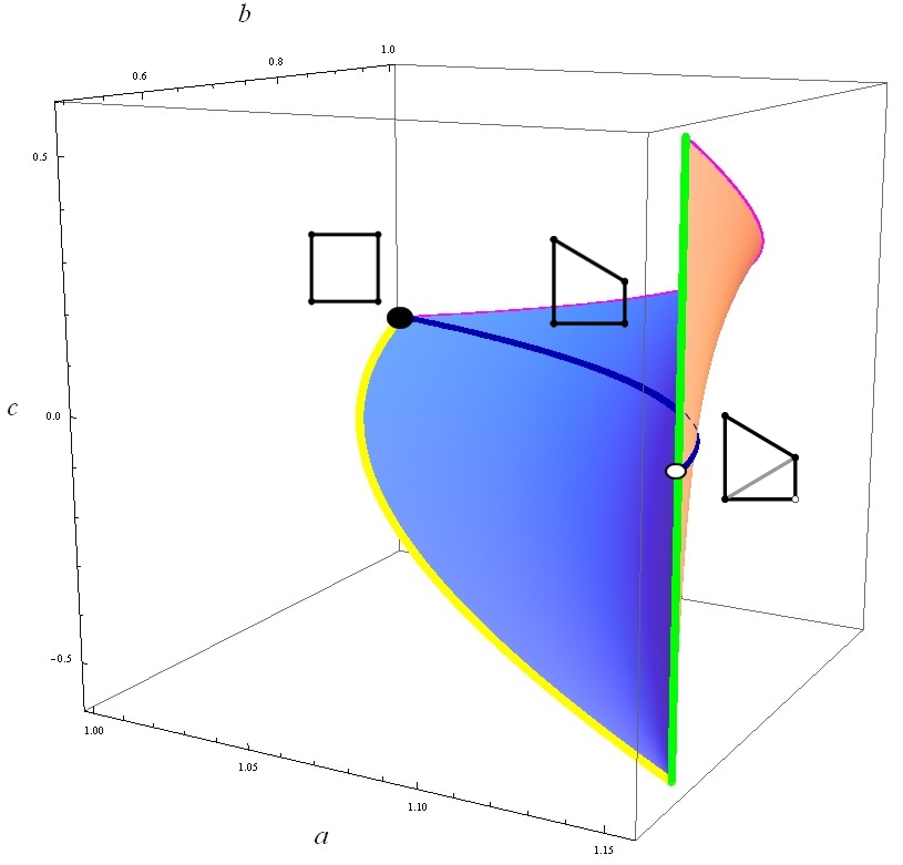
(a)                                                      (b)

Figure 4. (a) The region $\Omega_{r}$ and the the curve $D=0$ for the right trapezoid family in the $a-b$ plane. (b) The the curve $D=0$ for the right trapezoid family on the region $\Omega$.

Theorem 9.

The curve $D=0$ is a graph with respect to the variable $a$ in the region $\Omega_{r}$ (see Figure 4). In fact, $\partial D/\partial a$ evaluated at the curve $D=0$ restricted to $\Omega_{r}$ is negative.

Proof.

When $b=1$ equation $D=0$ becomes

$$\left(1-2\sqrt{2}\right)\left(\left(a^{2}+1\right)^{3/2}-1\right)\left(a^{3}-\left(a^{2}-2a+2\right)^{3/2}\right)=0,$$

which has a unique real solution with $a\geq 1$, the solution $a=1$. After straightforward computations we see that substituting $a=a_{2}(b)$ into $D$ we get a function of $b$ that is zero at $b=1$ and $b=1/\sqrt{3}$ and positive for $b\in(1/\sqrt{3},1)$. In a similar way substituting $a=a_{1}(b)$ into $D$ we get a function of $b$ that is zero at $b=0$ and $b=1/\sqrt{3}$ and negative for $b\in(1/\sqrt{3},1]$. Therefore each curve in $\Omega_{r}$ joining a point of the curve $a_{1}(b)$ with a point of the curve $a_{2}(b)$ has at least a point with $D=0$. Therefore there exist al least one set in $\Omega_{r}$ satisfying $D=0$. Next we see that this set is a graph in the variable $a$ that joins the points $(1,1)$ and $(2/\sqrt{3},1/\sqrt{3})$, see Figure 4(a).

By simple computations we get

$$\frac{\partial D}{\partial a}=\frac{\partial D}{\partial r_{12}}\frac{\partial r_{12}}{\partial a}+\frac{\partial D}{\partial r_{23}}\frac{\partial r_{23}}{\partial a}+\frac{\partial D}{\partial r_{24}}\frac{\partial r_{24}}{\partial a},$$

where

$$\frac{\partial r_{12}}{\partial a} = 1,$$

$$\frac{\partial r_{23}}{\partial a} = \frac{a-b}{r_{23}}=\frac{r_{12}-r_{34}}{r_{23}},$$

$$\frac{\partial r_{24}}{\partial a} = \frac{a}{r_{24}}=\frac{r_{12}}{r_{24}},$$

and

$$\frac{\partial D}{\partial r_{12}} = -3r_{12}^{2}\left(r_{13}^{3}-r_{23}^{3}\right)\left(r_{24}^{3}-r_{34}^{3}\right)-3r_{12}^{2}\left(r_{24}^{3}-r_{14}^{3}\right)\left(r_{23}^{3}-r_{34}^{3}\right),$$

$$\frac{\partial D}{\partial r_{23}} = 3r_{23}^{2}\left(r_{13}^{3}-r_{12}^{3}\right)\left(r_{24}^{3}-r_{14}^{3}\right)+3r_{23}^{2}\left(r_{12}^{3}-r_{14}^{3}\right)\left(r_{24}^{3}-r_{34}^{3}\right),$$

$$\frac{\partial D}{\partial r_{24}} = 3r_{24}^{2}\left(r_{13}^{3}-r_{12}^{3}\right)\left(r_{23}^{3}-r_{34}^{3}\right)-3r_{24}^{2}\left(r_{12}^{3}-r_{14}^{3}\right)\left(r_{13}^{3}-r_{23}^{3}\right).$$

Rearranging the terms in a convenient way $\partial D/\partial a$ can be written in terms of the mutual distances as

$$\frac{\partial D}{\partial a}=3(f_{1}+f_{2}+f_{3}+f_{4}+f_{5}+f_{6})$$

where

$$f_{1} = -r_{12}^{2}\left(r_{24}^{3}-r_{14}^{3}\right)\left(r_{23}^{3}-r_{34}^{3}\right),$$

$$f_{2} = -r_{12}^{2}\left(r_{13}^{3}-r_{23}^{3}\right)\left(r_{24}^{3}-r_{34}^{3}\right),$$

$$f_{3} = r_{23}(r_{12}-r_{34})\left(r_{13}^{3}-r_{12}^{3}\right)\left(r_{24}^{3}-r_{14}^{3}\right),$$

$$f_{4} = r_{23}(r_{12}-r_{34})\left(r_{12}^{3}-r_{14}^{3}\right)\left(r_{24}^{3}-r_{34}^{3}\right),$$

$$f_{5} = r_{12}r_{24}\left(r_{13}^{3}-r_{12}^{3}\right)\left(r_{23}^{3}-r_{34}^{3}\right),$$

$$f_{6} = -r_{12}r_{24}\left(r_{12}^{3}-r_{14}^{3}\right)\left(r_{13}^{3}-r_{23}^{3}\right).$$

Next, we will see that at the points of $\Omega_{r}$ satisfying $D=0$ the following conditions hold: $f_{1}+f_{4}<0$, $f_{2}+f_{5}<0$ and $f_{3}+f_{6}\leqslant 0$. Therefore $\partial D/\partial a$ evaluated at the curve $D=0$ restricted to $\Omega_{r}$ is negative.

From $D=0$ we get

$$\left(r_{24}^{3}-r_{14}^{3}\right)\left(r_{23}^{3}-r_{34}^{3}\right)=\frac{\left(r_{12}^{3}-r_{14}^{3}\right)\left(r_{13}^{3}-r_{23}^{3}\right)\left(r_{24}^{3}-r_{34}^{3}\right)}{r_{13}^{3}-r_{12}^{3}}.$$

Then $f_{1}+f_{4}$ can be written as

$$f_{1}+f_{4}=\frac{g_{1}\left(r_{12}^{3}-r_{14}^{3}\right)\left(r_{24}^{3}-r_{34}^{3}\right)}{r_{13}^{3}-r_{12}^{3}},$$

where

$$g_{1}=-r_{34}r_{23}\left(r_{13}^{3}-r_{12}^{3}\right)-r_{12}(r_{12}-r_{23})\left(r_{12}r_{23}(r_{12}+r_{23})+r_{13}^{3}\right).$$

Since $r_{13}>r_{12}\geqslant r_{23}$ on $\Omega_{r}$ and $g_{1}<0$ on $\Omega_{r}$, it follows that $f_{1}+f_{4}<0$ evaluated at the curve $D=0$ restricted to $\Omega_{r}$.

Proceeding as above, using that $D=0$ expression $f_{2}+f_{5}$ can be written as

$$f_{2}+f_{5}=\frac{g_{2}\left(r_{13}^{3}-r_{12}^{3}\right)\left(r_{23}^{3}-r_{34}^{3}\right)}{r_{12}^{3}-r_{14}^{3}},$$

where

$$g_{2}=-r_{12}(r_{24}-r_{12})(r_{14}^{3}+r_{12}^{2}r_{24}+r_{12}r_{24}^{2}).$$

Since $r_{24}>r_{12}$ on $\Omega_{r}$, $g_{2}<0$ on $\Omega_{r}$, we obtain that $f_{2}+f_{5}<0$ evaluated at the curve $D=0$ restricted to $\Omega_{r}$.

Finally, using that $D=0$ expression $f_{3}+f_{6}$ can be written as

$$f_{3}+f_{6}=\frac{g_{3}\left(r_{13}^{3}-r_{12}^{3}\right)\left(r_{24}^{3}-r_{14}^{3}\right)}{r_{24}^{3}-r_{34}^{3}},$$

where

$$g_{3}=-r_{24}r_{12}(r_{23}^{3}-r_{34}^{3})+r_{23}(r_{12}-r_{34})(r_{24}^{3}-r_{34}^{3}).$$

There exists a curve in $\Omega_{r}$ such that $g_{3}=0$, so the previous arguments are not valid to prove that $f_{3}+f_{6}$ evaluated at the curve $D=0$ restricted to $\Omega_{r}$ is negative.

In order to avoid the last obstacle, by using resultants we will prove that there are no values $(a,b)$ in the interior of $\Omega_{r}$ for which $D$ and $g_{3}$ are zero simultaneously.

Let $\mathrm{Res}[P,Q,x]$ denote the resultant of the polynomials $P(x,y)$ and $Q(x,y)$ with respect to $x$. The resultant $\mathrm{Res}[P,Q,x]$ is a polynomial in the variable $y$ satisfying the following property: if $(x,y)=(x^{*},y^{*})$ is a solution of system $P(x,y)=0$, $Q(x,y)=0$ then $y=y^{*}$ is a zero of $\mathrm{Res}[P,Q,x]$. In other words, the set of zeroes of $\mathrm{Res}[P,Q,x]$ contains the components $y$ of all solutions of the system $P(x,y)=0$ and $Q(x,y)=0$. We observe that it may contain additional solutions that are not related with the solutions of the system $P(x,y)=0$ and $Q(x,y)=0$.

Let

(18) $$\begin{array}[]{l}e_{1}=e_{1}(a,b,r_{13},r_{23},r_{24})=0,\\ e_{2}=e_{2}(a,b,r_{23},r_{24})=0,\end{array}$$

be the system defined by the two equations $D=0$ and $g_{3}=0$ after performing the substitutions $r_{12}=a$, $r_{14}=1$ and $r_{34}=b$. Here we think that the mutual distances $r_{13}$, $r_{23}$ and $r_{24}$ are the positive solutions of system

$$e_{3}=e_{3}(a,b,r_{13}) = r_{13}^{2}-(b^{2}+1)=0,$$

$$e_{4}=e_{4}(a,b,r_{23}) = r_{23}^{2}-((a-b)^{2}+1)=0,$$

$$e_{5}=e_{5}(a,b,r_{24}) = r_{24}^{2}-(a^{2}+1)=0.$$

Using resultants we eliminate the variables $r_{13}$, $r_{23}$ and $r_{24}$ from the equations (18) in the following way. We eliminate the variable $r_{13}$ from $e_{1}$ by doing the resultant

$$R_{1}=\mathrm{Res}[e_{1},e_{3},r_{13}].$$

Then we eliminate the variable $r_{23}$ from $R_{1}$ and $e_{2}$ by doing the resultants

$$S_{1}=\mathrm{Res}[R_{1},e_{4},r_{23}],\qquad S_{2}=\mathrm{Res}[e_{2},e_{4},r_{23}],$$

and the variable $r_{24}$ from $S_{1}$ and $S_{2}$ by doing the resultants

$$T_{1}=\mathrm{Res}[S_{1},e_{5},r_{24}],\qquad T_{2}=\mathrm{Res}[S_{2},e_{5},r_{24}].$$

Here $T_{1}=16a^{2}b^{2}\widetilde{T}_{1}$ and $T_{2}=b^{4}\widetilde{T}_{2}$, were $\widetilde{T}_{1}$ and $\widetilde{T}_{2}$ are polynomials of total degree 64 and 16, respectively, in the variables $a$ and $b$. Note that by the properties of resultants the set of solutions of the new system of equations $\widetilde{T}_{1}=0$, $\widetilde{T}_{2}=0$ contains all solutions with $a,b\neq 0$ of system (18), or equivalently all the solutions with $a,b\neq 0$ of system $D=0$, $g_{3}=0$ (thinking $D$ and $g_{3}$ as a function of $a,b$ via the mutual distances $r_{ij}$).

Now we solve system $\widetilde{T}_{1}=0$, $\widetilde{T}_{2}=0$ by using resultants again. We compute $\mathrm{Res}[\widetilde{T}_{1},\widetilde{T}_{2},a]$ and we get the polynomial

(19) $$\begin{array}[]{rcl}W(b)&=&(b-1)^{16}b^{96}\left(b^{2}+1\right)^{20}\left(b^{2}-b+1\right)^{4}\left(b^{2}+b+1\right)^{16}\\ &&\left(3b^{2}-4\right)^{2}\left(21b^{4}+12b^{2}+16\right)^{4}\left(21b^{4}+24b^{2}+16\right)^{2}\\ &&W_{1}(b)\,W_{2}(b)\,W_{3}(b)\,W_{4}(b),\end{array}$$

where $W_{1}$, $W_{2}$, $W_{3}$ and $W_{4}$ are polynomials of degrees 162, 202, 210, and 214 respectively. From properties of resultants the set of zeroes of $W$ contains the component $b$ of all the solutions of system $\widetilde{T}_{1}=0$, $\widetilde{T}_{2}=0$. Recall that we are only interested in solutions belonging to $\Omega_{r}$, so we only consider zeroes with $1/\sqrt{3}<b\leqslant 1$. We compute analytically the zeroes of the first eight factors of $W$ and numerically the zeroes of the remaining four factors of $W$ and we get the following solutions with $1/\sqrt{3}<b\leqslant 1$

$$b =0.61283303\dots,\quad b=0.69216326\dots,$$

$$b =0.71614387\dots, b=0.76874157\dots,$$

$$b =0.79099409\dots, b=0.82966657\dots,$$

$$b =0.91953907\dots, b=1.$$

Next we compute $\mathrm{Res}[\widetilde{T}_{1},\widetilde{T}_{2},b]$ and we get the polynomial

(20) $$\begin{array}[]{rcl}w(a)&=&(a-1)^{24}a^{64}\left(a^{2}+1\right)^{40}\left(a^{2}-a+1\right)^{4}\left(a^{2}+a+1\right)^{8}\\ &&\left(3a^{2}-1\right)^{2}\left(21a^{4}+6a^{2}+1\right)^{4}\left(21a^{4}+54a^{2}+49\right)^{2}\\ &&w_{1}(a)\,w_{2}(a)\,w_{3}(a)\,w_{4}(a),\end{array}$$

where $w_{1}$, $w_{2}$, $w_{3}$ and $w_{4}$ are polynomials of degrees 162, 202, 210, and 214 respectively. The set of zeroes of $w$ contains the component $a$ of all the solutions of system $\widetilde{T}_{1}=0$, $\widetilde{T}_{2}=0$. Since we are only interested in solutions belonging to $\Omega_{r}$, we only consider zeroes with $1\leqslant a\leqslant\sqrt{2}$. As above we compute analytically the zeroes of the first eight factors of $w$ and numerically the zeroes of the remaining four factors of $w$ and we get the following solutions with $1\leqslant a\leqslant\sqrt{2}$

$$a =1,\phantom{07124596\dots}\ \qquad a=1.04304633\dots,$$

$$a =1.07124596\dots,\qquad a=1.08484650\dots,$$

$$a =1.09217286\dots,\qquad a=1.10559255\dots,$$

$$a =1.16459040\dots.\qquad$$

We consider $D$ and $g_{3}$ as a function of $(a,b)$ by substituting the expressions of the mutual distances $r_{ij}$. The possible solutions $(a,b)$ of system $D=0$, $g_{3}=0$ are the pairs $(a,b)=(a^{*},b^{*})$ formed by a zero $a^{*}$ of $w$ with $a^{*}\in[1,\sqrt{2}]$, and a zero $b^{*}$ of $W$ with $b^{*}\in(1/\sqrt{3},1]$. Substituting all possible pairs $(a,b)=(a^{*},b^{*})$ into $D=0$, $g_{3}=0$ we see that $(a,b)=(1,1)$ is the unique pair that provides a solution of the system. This point belongs to the boundary of $\Omega_{r}$. Therefore the function $g_{3}$ does not change its sign on the solutions of $D=0$ that belong to $\Omega_{r}$.

It is easy to the check that the point $(a,b)=(2/\sqrt{3},1/\sqrt{3})$, which belongs to the boundary of $\Omega_{r}$, satisfies $D=0$. Moreover the function $g_{3}$ evaluated at $(a,b)=(2/\sqrt{3},1/\sqrt{3})$ is negative. Hence $g_{3}\leqslant 0$ in $\Omega_{r}$. This end the proof of the theorem. ∎

In short, the set of realizable right trapezoid central configurations is

$$\Omega_{r}^{\prime}=\{(a,b,c)\in\Omega_{r}\>:\>D=0\},$$

and it is plotted in Figure 4. In Figure 5 we plot the masses along the right trapezoid family parameterized by the parameter $a$. We note that the limit case $(a,b)=(1,1)$ correspond to the square with equal masses, and the limit case $(a,b)=(2/\sqrt{3},1/\sqrt{3})$ corresponds to a right trapezoid central configurations with masses $m_{1}=1$, $m_{4}=0$ and

(21) $$\begin{split}m_{2}=&\frac{7\left(8\sqrt{3}-9\right)\left(49+8\sqrt{7}\right)}{2511}=0.94993335\dots,\\[5.0pt] m_{3}=&\frac{2}{63}\left(8\sqrt{3}-9\right)=0.15417163\dots,\end{split}$$

such that the masses $m_{1},m_{2},m_{3}$ form an equilateral triangle with edge length $2/\sqrt{3}$.

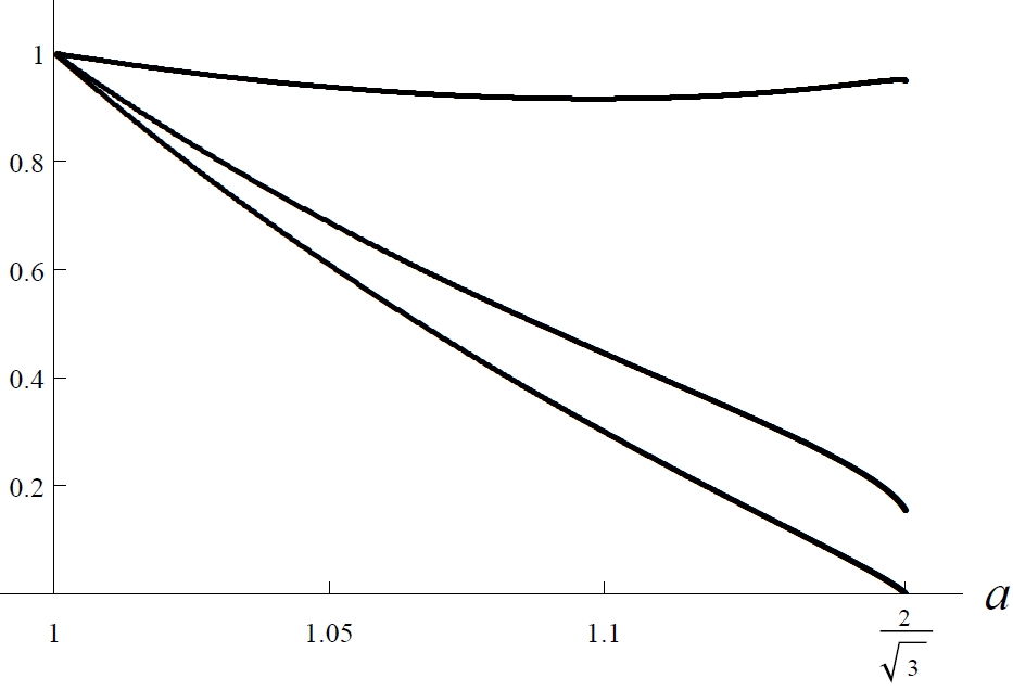
Figure 5. The plot of the masses $m_{2}$ (upper line), $m_{3}$ (medium line) and $m_{4}$ (bottom line) along the right trapezoid family.

7. Trapezoid CC with a couple of equal masses

In this section we will study the trapezoid CC with a pair of equal masses. In [15] Cors and Roberts shown that for a given order of the mutual distances in any co–circular central configuration the set of masses is completely ordered. A similar result for the trapezoid central configurations has been obtained recently by Santoprete [40]. Although in that case the masses are not totally ordered. With our particular choice of labeling, from [40] any trapezoid central configuration satisfies

(22) $$m_{4}\leq m_{3}\leq m_{1}=1\qquad m_{4}\leq m_{2}.$$

Moreover, also from Santoprete [40], we know that if $m_{3}=m_{1}=1$ or $m_{2}=m_{4}$, then the central configuration is a rhombus and the remaining two masses have to be equal. And if $m_{3}=m_{4}$, then the central configuration is an isosceles trapezoid and again the two remaining masses are necessarily equal. Figure 6 shows the full set of masses for which a trapezoid central configuration exist.

Figure 6. The image of $\Omega$ in $m_{2}m_{3}m_{4}$–space under equations (14), (15) and (16) with $m_{1}=1$.

From the previous results only two cases of trapezoid central configuration with only a pair of equal masses remains unknown, namely, $m_{2}=m_{3}$ and $m_{2}=m_{1}=1$. In the next two subsections we are going to show the existence of these two classes of trapezoid central configuration. Something remarkable is that we will proved analytically the existence of non–symmetric trapezoid central configurations with two equal masses. As far as we know this result was known numerically, but we think that is the first time that this result is proved analytically in the four–body problem.

Now we study the value of masses along the boundary of $\Omega$.

The equilateral triangle family. By substituting the points of $\mathcal{C}_{1}$ into (14), (15) and (16) we get $m_{4}=0$ and

(23) $$m_{2}=\mu_{2}(c)=\frac{\left(8\sqrt{3}-9k_{1}^{3}\right)k_{2}^{3}}{9k_{1}^{3}\left(k_{2}^{3}-8\right)},\quad m_{3}=\mu_{3}(c)=\frac{2\left(\sqrt{3}-3c\right)^{2}\left(8\sqrt{3}-9k_{1}^{3}\right)}{27\left(\sqrt{3}c+1\right)k_{1}^{3}k_{2}^{2}},$$

where $k_{1}=\sqrt{c^{2}+1}$ and $k_{2}=\sqrt{3c^{2}-4\sqrt{3}c+7}$. The function $\mu_{2}$ is defined for all $c\in[-1/\sqrt{3},1/\sqrt{3})$, $\mu_{2}(-1/\sqrt{3})=0$ and $\mu_{2}(c)\to 1$ when $c\to 1/\sqrt{3}$; moreover it is increasing for $c\in[-1/\sqrt{3},c_{0})$, it has a maximum at $c_{0}=0.27448350\dots$ with $\mu_{2}(c_{0})=1.0912476\dots$ and it is decreasing for $c\in(c_{0},1/\sqrt{3})$. The function $\mu_{3}$ is defined for all $c\in(-1/\sqrt{3},1/\sqrt{3}]$, $\mu_{3}(1/\sqrt{3})=0$, $\mu_{3}(c)\to 1/2$ when $c\to-1/\sqrt{3}$ and it is decreasing for $c\in(-1/\sqrt{3},1/\sqrt{3}]$. The plot of the masses on $\mathcal{C}_{1}$ is given in Figure 7 (a).

The rhombus family. By substituting the points of $\mathcal{C}_{2}$ into (14), (16) and (17) we get $m_{1}=m_{3}=1$ and

$$m_{2}=m_{4}=\mu_{r}(c)=-\frac{\left((c-k)^{2}+1\right)^{3/2}\left(\left((c+k)^{2}+1\right)^{3/2}-k^{3}\right)}{\left(k^{3}-\left((c-k)^{2}+1\right)^{3/2}\right)\left((c+k)^{2}+1\right)^{3/2}},$$

where $k=\sqrt{1+c^{2}}$. Note that on the rhombus family expression (15) is not well defined and we should take expression (17) instead of it. We can see that $\mu_{r}$ is an increasing function defined for all $c\in[-1/\sqrt{3},0]$, such that $\mu_{r}(-1/\sqrt{3})=0$ and $\mu_{r}(0)=1$. The plot of the masses on $\mathcal{C}_{2}$ is given in Figure 7 (b).

The isosceles trapezoid family. On the isosceles trapezoid family we know that $m_{1}=m_{2}=1$ and $m_{3}=m_{4}=\mu$ (see for instance [15]), but since we do not have an explicit expression of the solutions of $f(b,c)=0$, we cannot give the explicit expression of $\mu$ as a function of the parameter $c$. Studying numerically the function $\mu$ we see that it is a decreasing function in $c\in(0,1/\sqrt{3})$ such that $\mu\to 1$ when $c\to 0$ and $\mu\to 0$ when $c\to 1/\sqrt{3}$. The plot of the masses on $\mathcal{C}_{3}$ is given in Figure 7 (c).

Note that if we approach to $P_{2}$ over the set $\mathcal{C}_{2}$ then $m_{3}\to 1$, whereas if we approach to $P_{2}$ over the set $\mathcal{C}_{1}$ then $m_{3}\to 1/2$. Thus the limit of $m_{3}$ as we approach to $P_{2}$ depends on the path you take and $m_{3}$ has a non removable discontinuity at $P_{2}$.

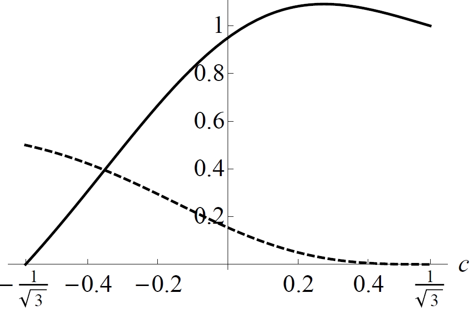
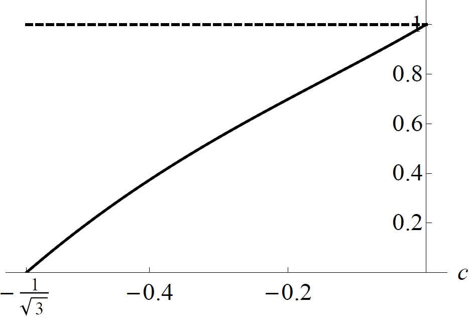
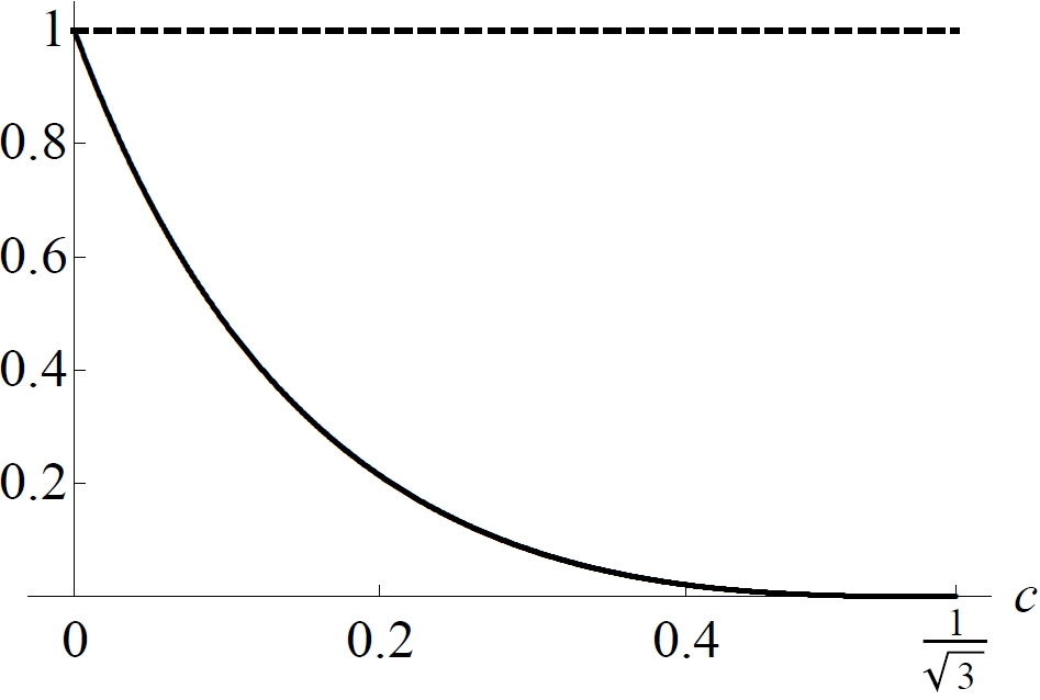
(a)	(b)	(c)

Figure 7. (a) The plot of the masses $m_{2}$ (continuous line) and $m_{3}$ (dashed line) on the boundary $\mathcal{C}_{1}$. (b) The plot of the masses $m_{2}=m_{4}$ (continuous line) and $m_{1}=m_{3}=1$ (dashed line) along the rhombus family. (c) The plot of the masses $m_{1}=m_{2}=1$ (dashed line) and $m_{3}=m_{4}$ (continuous line) along the isosceles trapezoid family.

7.1. $m_{2}=m_{3}$

Take $f=m_{2}-m_{3}$. We are interested in the solutions of $f=0$. On $\mathcal{C}_{2}$ (corresponding to the rhombus family) we have $r_{12}=r_{23}=r_{34}=r_{14}$ and $m_{1}=m_{3}=1$.

We know from equation (14) that on $\mathcal{C}_{2}$

(24) $$m_{2}=\frac{r_{23}^{3}r_{24}^{3}\,(r_{13}^{3}-r_{14}^{3})}{r_{13}^{3}r_{14}^{3}\,(r_{24}^{3}-r_{23}^{3})}=\frac{r_{24}^{3}\,(r_{13}^{3}-r_{12}^{3})}{r_{13}^{3}\,(r_{24}^{3}-r_{12}^{3})}.$$

Therefore

$$m_{2}<1 \iff r_{24}^{3}\,(r_{13}^{3}-r_{12}^{3})<r_{13}^{3}\,(r_{24}^{3}-r_{12}^{3})$$

$$\iff -r_{24}^{3}\,r_{12}^{3}<-r_{13}^{3}\,r_{12}^{3}\iff r_{24}^{3}>r_{13}^{3}.$$

The last inequality follows from the fact that $r_{24}>r_{13}>1$. Therefore on $\mathcal{C}_{2}$ we have $f=m_{2}-m_{3}<0.$

Now on $\mathcal{C}_{3}$ (corresponding to the isosceles trapezoid family) we have $r_{23}=r_{14}$, $r_{24}=r_{13}$ and $m_{1}=m_{2}=1$. We also know that on this family $m_{3}=m_{4}$.

$$m_{3}=m_{4}<1 \iff \frac{r_{34}^{2}\,(r_{13}^{3}-r_{12}^{3})}{r_{12}^{2}\,(r_{13}^{3}-r_{34}^{3})}$$

$$\iff r_{34}^{2}(r_{13}^{3}-r_{12}^{3})<r_{12}^{2}(r_{13}^{3}-r_{34}^{3})$$

$$\iff -r_{13}^{3}(r_{12}^{2}-r_{34}^{2})<r_{12}^{2}r_{34}^{2}(r_{12}-r_{34})$$

$$\iff -r_{13}^{3}(r_{12}-r_{34})(r_{12}+r_{34})<r_{12}^{2}r_{34}^{2}(r_{12}-r_{34})$$

$$\iff -r_{13}^{3}(r_{12}+r_{34})<r_{12}^{2}r_{34}^{2}.$$

That is, on $\mathcal{C}_{3}$ we have $f=m_{2}-m_{3}>0.$ Therefore for any given path connecting $\mathcal{C}_{2}$ and $\mathcal{C}_{3}$ in $\Omega$, there exist $(a,b,c)\in\Omega$ such that $f=0$ or equivalently $m_{2}=m_{3}$.

Numerically we show that for any fixed path connecting $\mathcal{C}_{2}$ and $\mathcal{C}_{3}$ in $\Omega$ the solution of $f=0$ is unique. Curve representing the zeros of $f$ in $\Omega$ goes from $P_{3}$ to $(2/\sqrt{3},1/\sqrt{3},-0.351839354\dots)\in\mathcal{C}_{1}$ (see Figure 8). To verify the last statement, we observe that the function $f$ on $\mathcal{C}_{1}$ becomes

$$f=\frac{\left(\frac{8}{3\sqrt{3}}-\left(c^{2}+1\right)^{3/2}\right)\left(-\frac{6\left(\frac{1}{\sqrt{3}}-c\right)^{2}}{8-\left(3c^{2}-2\sqrt{3}c+1\right)^{3/2}}-\frac{\left(3c^{2}-4\sqrt{3}c+7\right)^{3/2}}{8-\left(3c^{2}-4\sqrt{3}c+7\right)^{3/2}}\right)}{\left(c^{2}+1\right)^{3/2}}.$$

We apply Sturm Theorem to conclude that $f=0$, as a polynomial of degree 24, has a unique real solution in $c\in(-1/\sqrt{3},1/\sqrt{3})$, namely $c=-0.351839354\dots$

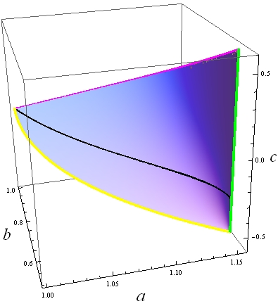
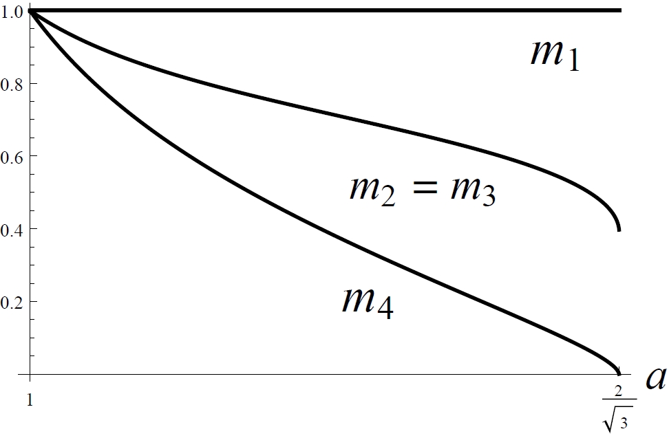
Figure 8. (a) In black, the curve $m_{2}=m_{3}$ on the region $\Omega$. (b) The curves $m_{1}=1$, $m_{2}=m_{3}$, and $m_{4}$ parametrized by $a$ on the curve in (a).

7.2. $m_{2}=m_{1}=1$

It is clear that $m_{2}=m_{1}=1$ along the isosceles trapezoid central configuration family, that is, on the boundary $\mathcal{C}_{3}$. Moreover $m_{1}=m_{2}=m_{3}=m_{4}=1$ on $P_{3}$, that is, on the square configuration, and $m_{2}-m_{1}<0$ on $\mathcal{C}_{2}\cup P_{2}$.

On the boundary $\mathcal{C}_{1}\cup\{P_{1},P_{2}\}$ we have $m_{4}=0$ and $m_{1},m_{2}$ and $m_{3}$ at the vertices of an equilateral triangle. Let $m_{2}=\mu_{2}(c)$ be the value of the mass $m_{2}$ on $\mathcal{C}_{1}$, see (23). We have seen that $\mu_{2}(c)\to 1$ when $c\to 1/\sqrt{3}$, and that $\mu_{2}$ is decreasing for $c\in(c_{0},1/\sqrt{3})$ with $c_{0}=0.27448350\dots$, so $m_{2}-m_{1}>0$ near $P_{1}$. On the other hand at the point $Q=(2/\sqrt{3},1/\sqrt{3},0)$ corresponding to the right trapezoid we have $m_{2}=0.15417163\dots<1$, see (21) which implies $m_{2}-m_{1}<0$. Therefore there exists a point $T$ on $\mathcal{C}_{1}$ such that $m_{2}=m_{1}$. Again applying Sturm Theorem to a polynomial of degree 22 in $c$, we can conclude that $T$ is unique, and its coordinates are $(2/\sqrt{3},1/\sqrt{3},c_{1})$ where $c_{1}=0.0517595932\dots$

Let $\widetilde{\mathcal{C}}_{1}=\{(a,b,c)\in\mathcal{C}_{1}\>:\>c<c_{1}\}$ and ${\widetilde{\mathcal{C}}_{1}}^{\prime}=\{(a,b,c)\in\mathcal{C}_{1}\>:\>c>c_{1}\}$. Therefore, for any given path connecting $\widetilde{\mathcal{C}}_{1}$ and $P_{3}\cup\mathcal{C}_{3}\cup P_{1}\cup{\widetilde{\mathcal{C}}_{1}}^{\prime}$ in $\Omega$, there exist $(a,b,c)\in\Omega$ such that $m_{2}=m_{1}=1$.

Numerically we show that for any fixed path connecting $\widetilde{\mathcal{C}}_{1}$ and $P_{3}\cup\mathcal{C}_{3}\cup P_{1}\cup{\widetilde{\mathcal{C}}_{1}}^{\prime}$ in $\Omega$ the solution of $m_{2}-1=0$ is unique. Curve representing the zeros of $m_{2}-1$ joins the boundaries $\mathcal{C}_{3}$ and $\mathcal{C}_{1}$. This curve goes from $(1.13102016\dots,0.896392974\dots,0.234627188\dots)\in\mathcal{C}_{3}$ to $(2/\sqrt{3},1/\sqrt{3},c_{1})\in\mathcal{C}_{1}$ (see Figure 9 (a)). The values of the masses $m_{3}$ and $m_{4}$ along this curve are plotted in Figure 9 (b).

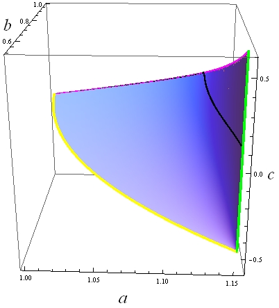
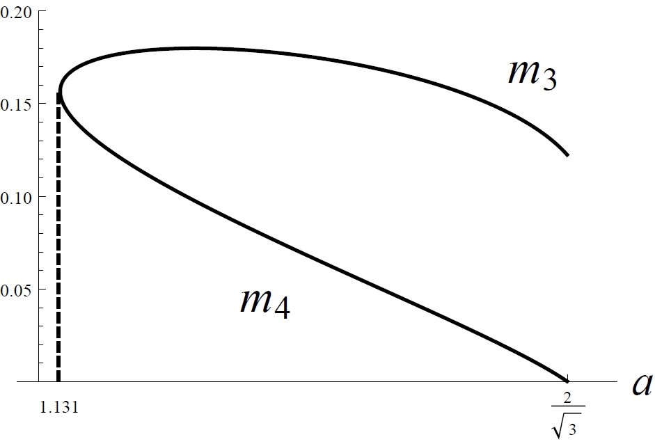
(a)                                                      (b)

Figure 9. (a) In black, the curve $m_{2}=1$ on the region $\Omega$. (b) The curves of $m_{3}$ and $m_{4}$, parameterized by $a$ on the curve in (a).

8. Conclusions

Using the positions of the masses we have classified the set of trapezoid central configurations. This set is a two–dimensional surface whose boundaries are known families consisting in a rhombus, an isosceles trapezoid and an equilateral triangle with a zero mass off the triangle. Although a specific ordering of the masses has not hold for any trapezoid central configuration, we can split the two–dimensional surface in three disjoint regions where the set of masses is totally ordered. Somewhat we must remark that we have proved analytically the existence of non–symmetric trapezoid central configurations with a pair of equal masses.

There exist a one–parameter family of right trapezoid central configurations that also splits the two–dimensional surface in two disjoint regions, namely the acute and the obtuse regions. Along such a non–symmetric family the masses are completely ordered, that is, the family belong to one of the previous three regions, concretely the middle one, where the set of masses is totally ordered. Moreover, when the pair of equal masses belong to biggest parallel side, only acute trapezoid central configurations are allow. On the other hand, when the two equal masses belongs to the non–parallel side, only obtuse trapezoid central configurations are allow.

Acknowledgements

The first three authors are partially supported by a FEDER-MINECO grant MTM2016-77278-P and a MINECO grant MTM2013-40998-P. The second and third authors are also supported by an AGAUR grant number 2014SGR-568. The fourth author is supported by Fondo Mexicano de Cultura A.C.

References

- [1] Albouy, A., Symétrie des configurations centrales de quatre corps, C. R. Acad. Sci. Paris, 320 (1995), 217–220.
- [2] Albouy, A., The symmetric central configurations of four equal masses, Contemp. Math., 198 (1996), 131–135.
- [3] Albouy, A., On a paper of Moeckel on central configurations, Regul. Chaotic Dyn. 8 (2003), no. 2, 133-142.
- [4] Albouy, A., Chenciner, A., Le problème des corps et les distances mutuelles, Invent. Math. 131 (1998), 151-184.
- [5] Albouy, A. and Fu, Y., Euler configurations and quasi polynomial systems, Regul. Chaotic Dyn. 12 (2007), 39–55.
- [6] Albouy, A., Fu, Y. and Sun, S., Symmetry of planar four–body convex central configurations, Proc. R. Soc. Lond. Ser. A Math. Phys. Eng. Sci., 464 (2008), 1355–1365.
- [7] Albouy, A. and Kaloshin, V., Finiteness of central configurations of five bodies in the plane, Ann. of Math. (2) 176 (2012), 535–588.
- [8] Albouy, A., Fu, Y. and Sun, S., Symmetry of planar four-body convex central configurations, Proc. R. Soc. Lond. Ser. A 464 (2008), no. 2093, 1355–1365.
- [9] Álvarez, M. and Llibre, J., The symmetric central configurations of a –body problem with masses , Appl. Math. and Comp. 219 (2013), 5996–6001.
- [10] Arenstorf, R.F., Central configurations of four bodies with one inferior mass, Cel. Mechanics 28 (1982), 9–15.
- [11] Barros, J.F. and Leandro, E.S.G., The Set of Degenerate Cetral Configurations in the Planar Restricted Four–Body Problem, SIAM Journal on Mathematical Analysis 43 (2011), 634–661.
- [12] Barros, J.F. and Leandro, E.S.G., Bifurcations and Enumeration of Classes of Relative Equilibria in the Planar Restricted Four–Body Problem, SIAM Journal on Mathematical Analysis 46 (2014), 1185–1203.
- [13] Bernat, J., Llibre, J. and Perez–Chavela, E., On the planar central configurations of the –body problem with three equal masses, Dyn. Contin. Discrete Impuls. Syst. Ser. A Math. Anal., 16 (2009), 1–13.
- [14] Corbera, M. and Llibre, J. Central configurations of the –body problem with masses and small, Appl. Math. Comput. 246 (2014), 121–147.
- [15] Cors J.M. and Roberts G.E., Four-body co-circular central configurations, Nonlinearity 25 (2012), 343–370.
- [16] Deng, Y., Li, B. and and Zhang, S., Four-body central configurations with adjacent equal masses, arXiv: 1608.06206v1, 2016.
- [17] Dziobek, O., Über einen merkwürdigen Fall des Vielkörperproblems, Astro. Nach. 152 (1900), 32–46.
- [18] L. Euler, De moto rectilineo trium corporum se mutuo attahentium, Novi Comm. Acad. Sci. Imp. Petrop., 11 (1767), 144–151.
- [19] Fernandes, A.C., Llibre, J. and Mello,L.F., Convex central configurations of the –body problem with two pairs of equal masses, to appear in Archive for Rational Mechanics and Analysis.
- [20] Gannaway, J.R., Determination of all central configurations in the planar –body problem with one inferior mass, Ph. D., Vanderbilt University, Nashville, USA, 1981.
- [21] Hampton, M., Co-circular central configurations in the four-body problem, EQUADIFF 2003 (Conference Proceedings), World Sci. Publ., Hackensack, NJ, (2005), 993–998.
- [22] Hagihara, Y., Celestial Mechanics, vol. 1, MIT Press, Massachusetts, 1970.
- [23] Hampton, M. and Moeckel, R., Finiteness of relative equilibria of the four-body problem, Invent. Math. 163 (2006), no.2, 289–312.
- [24] Kulevich, J.L., Roberts, G.E. and Smith, C. J., Finiteness in the planar restricted four–body problem, Qual. Theory Dyn. Syst. 8 (2009), 357–370.
- [25] Lagrange, J.L., Essai sur le problème de toris corps, Ouvres, vol. 6, Gauthier-Villars, Paris, 1873.
- [26] Leandro, E.S.G., Finiteness and bifurcation of some symmetrical classes of central configurations, Arch. Rational Mech. Anal. 167 (2003), 147–177.
- [27] Llibre, J., Posiciones de equilibrio realtivo del problema de 4 cuerpos, Publicacions Matemàtiques UAB 3 (1976), 73–88.
- [28] Llibre, J., On the number of central configurations in the -body problem, Celestial Mech. Dynam. Astronom. 50 (1991), 89–96.
- [29] Long, Y. and Sun, S., Four–Body Central Configurations with some Equal Masses, Arch. Rational Mech. Anal. 162 (2002), 24–44.
- [30] Long, Y., Admissible shapes of 4-body non-collinear relative equilibria, Adv. Nonlinear Stud. 3 (2003), no. 4, 495–509.
- [31] MacMillan, W.D. and Bartky, W., Permanent Configurations in the Problem of Four Bodies, Trans. Amer. Math. Soc. 34 (1932), no. 4, 838–875.
- [32] Meyer, K.R., Hall, G.R. and Offin, D., Introduction to Hamiltonian Dynamical Systems and the -Body Problem, 2nd ed., Applied Mathematica l Sciences 90, Springer, New York, 2009.
- [33] Moeckel, R., On central configurations, Mathematische Zeitschrift 205 (1990), no. 4, 499–517.
- [34] Moulton, F.R., The straight line solutions of bodies, Ann. of Math. 12 (1910), 1–17.
- [35] Palmore, J., Classifying relative equilibria, Bull. Amer. Math. Soc. 79 (1973), 904–907.
- [36] Pedersen, P., Librationspunkte im restringierten Vierk” orperproblem, Danske Vid. Selsk. Math.–Fys. 21 (1944), 1–80.
- [37] Pérez-Chavela E., and Santoprete, M., Convex Four-Body Central Configurations with Some Equal Masses, Arch. Rational Mech. Anal. 185 (2007), 481–494.
- [38] Saari, D.G., On the role and properties of central configurations, Celestial Mech., 21 (1980), 9–20.
- [39] Saari, D.G., Collisions, Rings, and Other Newtonian -Body Problems, CBMS Regional Conference Series in Mathematics, no. 104, Amer. Math. Soc., Providence, RI, 2005.
- [40] Santoprete, M., Four-body central configurations with one pair of opposite sides parallel, arXiv:1710.03124.
- [41] Schmidt, D., Central configurations and relative equilibria for the -body problem, Classical and celestial mechanics (Recife, 1993/1999), Princeton Univ. Press, Princeton, NJ, (2002), 1–33.
- [42] Simó, C., Relative equilibrium solutions in the four-body problem, Cel. Mechanics 18 (1978), 165–184.
- [43] Smale, S., Topology and mechanics I, Invent. Math. 10 (1970), 305–331.
- [44] Smale, S., Topology and mechanics II. The planar n-body problem, Invent. Math. 11 (1970), 45-64.
- [45] Smale, S., Mathematical problems for the next century, Math. Intelligencer 20 (1998), no. 2, 7–15.
- [46] Ruen, T., Own work, CC BY-SA 4.0, https://commons.wikimedia.org/w/index.php?curid=39504620.
- [47] Wintner, A., The Analytical Foundations of Celestial Mechanics, Princeton Math. Series 5, Princeton University Press, Princeton, NJ, 1941.
- [48] Xia,Z., Central configurations with many small masses, J. Differential Equations 91 (1991), 168–179.
- [49] Xia, Z., Convex central configurations for the -body problem, J. Differential Equations 200 (2004), 185–190.
- [50] Xie, Z., Isosceles trapezoid central configurations of the Newtonian four-body problem, Proc. R. Soc. Edinb., Sect. A, Math. 142 (2012), 665–672.