Self assembled linear polymeric chains with tuneable semiflexibility using isotropic interactions

Abstract

We propose a two-body spherically symmetric (isotropic) potential such that particles interacting by the potential self assemble into linear semiflexible polymeric chains without branching. By suitable control of the potential parameters we can control the persistence length of the polymer, and can even introduce a controlled number of branches. Thus we show how to achieve effective directional interactions starting from spherically symmetric potentials. The self assembled polymers have a exponential distribution of chain lengths akin to what is observed for worm-like micellar systems. On increasing particle density the polymeric chains self-organize to a ordered line-hexagonal phase where every chain is surround by six parallel chains, the transition is first order. On further increase in monomer density, the order is destroyed and we get a branched gel like phase. This potential can be used to model semi-flexible equilibrium polymers with tunable semiflexibility and excluded volume. The use of the potential is computationally cheap and hence, can be used to simulate and probe complex micellar dynamics with long chains. The potential also gives a plausible method of tuning colloidal interactions in experiments such that one can obtain self-assembling polymeric chains made up of colloids and probe polymer dynamics using an optical microscope.

I Introduction

The self-assembly of microscopic particles by tuning the interactions between them to obtain well-defined target structures has a well established direction of research in soft matter physics. The more recent focus in this area has evolved to heirarchical self assembly [1] as well as self-assembly with very many different constituent particles which will result in self-assembled structures of much higher complexity [2, 3, 4, 5, 6, 7, 8, 9, 10, 11, 12]. A line of investigation has been the self assembly of spherical particles with directional interactions (patchy colloids) and self assembly of particles with anisotropic shapes to obtain a zoo of different target structures and organizations [13]. Another line of studies has been to obtain directed interactions starting out from spherically symmetric interactions between suitably dressed isotropic particles [1, 14, 15, 16].

In particular, Mossa et.al. and others [15, 16, 17, 18] investigated the self assembly of spherical particles interacting with radially symmetric potentials with a short range attractive part and long range repulsive interactions (modelled by screened Coulomb interactions). On changing the relative contributions (range and strength) of these two parts of the interacting potential, they obtained clusters of particles with different organizations of particles within cluster, e.g., crystalline clusters as well as planar and linear extended aggregates of particles at temperature $T=0$ using energy minimization techniques. The organization also depended on the number of particles considered as it affects the average number of neighbours per particle in cluster. The range of attractive interaction was changed by changing the integer value of $n$ in the potential of the form $V_{att}=4\epsilon[(\sigma/r)^{2n}-(\sigma/r)^{n}]$, following the previous work of Vliegenhart et. al. [19]. Vliegenthart et. al. had various different ranges of the attractive potential of the form $V_{att}$ to investigate the role of the range of attractive minima to obtain liquid phases in the fluid-solid phase diagram.

Our aim is to develop a spherically symmetric model potential such that particles interacting by the potential self-assemble to linear equilibrium polymeric chains which are semiflexible; real life examples of such self assembled polymeric chains is worm-like micelles [20, 21, 22]. There exists quite a few coarse-grained models which describe self-assembling micellar chains [23, 24, 25, 26, 27, 28, 29, 30, 31, 6, 32, 33, 34]. Some use suitable rate constants to model joining and breaking of bonds between effective bead-spring monomers where only 2 bonds are allowed per monomer [25, 26, 27, 28, 29, 30, 31]. Other models have effective potentials for self assembly of particles into polymeric chains, where semiflexibility is incorporated by suitable angle dependent potentials [24, 32]. Branching or cluster formation is prevented by suitable choice of parameters of 3-body or 4 body potentials [6, 32, 33, 34]. The use of 3-body or 4-body potentials is cumbersome and computationally expensive, espcially when one wants to model systems of long chains to study interesting phenomenon such as shear banding [35, 36, 37, 38]. A simpler potential with just two-body spherically symmetric interaction potential would greatly help in modelling systems of long self assembled polymer chains, moreover, we would like to avoid branching or introduce branches in a controlled manner.

The spherically symmetric potential that we developed has three parts ($i$) a repulsive potential at very short distances of the form $(\sigma/r)^{24})$ which takes care of excluded volume interactions between self-assembling particles, where $r$ is the distance between 2 particles and $\sigma$ is the diameter ($ii$) a short range attractive potential $-(\sigma/r)^{12}$ at distances just beyond $\sigma$, and ($iii$) a screened Coulomb interaction of the form $\sim\frac{1}{r}e^{-r/R}$ with a suitable strength $\epsilon^{*}$ and range of interaction decided by $R$. We have two kinds of particles, A and B in equal ratios. A-A interactions and B-B are purely repulsive, modelled by screened Coulomb interactions ($iii$). The interaction between A-B particles is a combination of ($i$),($ii$) and ($iii$) such that A-B particles can attract each other when distances between the two are just above $\sigma$ and repel each other at longer distances. The form of the potentials are reminiscent of interaction between colloidal particles and can be used to make colloidal-polymers, even without the use of DNA-linkers [39]. This would open up possiblities to observe complex micellar dynamics e.g. rheochaos or shear banding to direct optical observation. In addition, because of the large size of the particles the dynamics would be much slower and can be tracked using standard optical microscopy techniques.

The rest of the manuscript is as follows. We describe the model potential and computational details in the next section: Methods. Then in the next Results-section we describe the various phases that we obtain as we change the number density of particles and temperature; we also describe how we control the branching properties and persistence length of the self assembled polymers. We conclude with discussions in the fourth and final section.

II Model

To develop an interaction potential between effective-monomers which self assemble to form a linear polymeric micellar chains, we avoid bead-spring potentials with suitable rate constants for bonds to join and break along the chain. Instead, we focus on developing a suitably modified Lennard Jones (LJ) type potential which encourages assembly of particles at short distances but also with a potential maxima at an appropriate longer distance which should discourage spherical clusters or branching. Moreover, right angles between bond-vectors in a triplet of monomers should be penalized. The monomers we have in mind could also be colloidal particles for which effective interaction can be tuned using changing surface properties or altering the counter-ion or salt densities around a charged colloid. To that end, we modify the LJ-type interaction by adding a Debye Huckel type screening potential between particles such that the total potential $V_{tot}$ is of the form $V_{tot}=\epsilon[(\sigma/r)^{2n}-(\sigma/r)^{n}+\epsilon^{*}e^{-r/R}/r]$ with exponent $n=12$, such that the potential looks akin to the potential shown in Fig.1(a). The $n=12$ potential have a sharper minima as compared to the usual LJ ($n=6$) potential, so that the peak due to the repulsive term can be shifted to lower values of $r$ just beyond the position of potential minima as shown in Fig.1a. The monomers self-assemble to form polymeric chains, however, contrary to our expectations, a large number of branches get inadvertently formed as the number density of monomers increases.

To prevent branching during the self assembly we introduce $2$ kinds of particles, (say) A and B; we maintain the interaction potential between A-A, A-B and B-B to be spherically symmetric. The interaction between a pair of A-B particles are kept to be of the same form as mentioned before, viz.,

$$V_{AB}(r)=\epsilon_{AB}\left[\left(\frac{\sigma}{r}\right)^{24}-\left(\frac{\sigma}{r}\right)^{12}+\epsilon^{*}_{AB}\frac{e^{-(r/R_{AB})}}{r}\right],\\ ..\forall r<r_{C}$$ (1)

where $\epsilon_{AB}=105\,k_{B}T$, $\epsilon^{*}_{AB}=16.81$, and $R_{AB}=0.25\sigma$. We model the interaction between similar particles (A-A or B-B) by screened Coulomb purely repulsive potential as given by Eqn. 2

$$V_{\alpha\alpha}(r)=\epsilon_{\alpha\alpha}\frac{e^{-(r/R_{\alpha\alpha})}}{r},\,\,\forall r<r_{C}$$ (2)

where $\alpha=A$ or $\alpha=B$; we choose $\epsilon_{AA}=\epsilon_{BB}$ and $r_{C}=3\sigma$. The parameter values are $\epsilon_{AA}=939.33\,k_{B}T$, $R_{AA}=R_{BB}=0.5\sigma$. This choice of parameters prevents identical particles from coming close to each other (energy at $r=2\sigma$ is $\approx 8k_{B}T$, refer Fig.2b), whereas A-B/B-A bound-pairs (effective-bonds) are easily formed due to the existence of the the potential minima in the interaction potential. We define A and B to be bonded if the distance between the particles is $<r_{b}=1.3\sigma$, where $r_{b}$ is the position of the potential maxima. If the A-B distance becomes greater than $r_{b}$ due thermal fluctuations, we define the effective bond to be broken. The A-B pairs in turn join up to form -A-B-A- chains. Right angled A-B-A configurations are discouraged due to strong repulsive energy between like particles at distances $\sqrt{2}\sigma$ (refer Eqn.2) resulting in semiflexible chains. Furthermore, a third $A$ particle cannot bond at right angles to $B$ to form a branch in a existing A-B-A configiuration due to the combined repulsion from the two $A$ particles. In a configuration where A-B-A forms a straight line, if a pair of A-B particles are kept at a fixed distance of $r_{12}=1.12\sigma$ the potential felt by the third $A$-particle as a combination of $V_{AA}$ and $V_{AB}$ as a function of distance $r$ ($r$ is measured from the particle $B$ at the center) is given in Fig.1$c$. As we show later, we can play with the parameters to allow limited amount of branching.

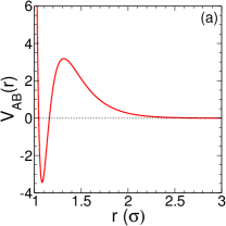
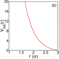
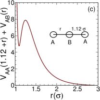
Figure 1: Representative plots of the potentials (a) $V_{ab}(r)$ acting between centers of $A$ and $B$ (b) $V_{aa}(r)$ acting between pair of $A-A$ or $B-B$ particles (c) $V_{AA}(1.12+r)+V_{AB}(r)$ for a linear triplet of $A-B-A$ (or $B-A-B$) particles, where the potential is plotted as a function of $r$, the distance of the third particle from central B particle. The distance between the first particle and central particle is kept fixed at $1.12\sigma$ (refer inset schematic diagram).

The excluded volume distance $\sigma$ of the $(\sigma/r)^{24}-(\sigma/r)^{12}$ potential sets the unit of length in our simulations, we use $\sigma=1$. All energies are measured in units of the thermal energy $k_{B}T$ ($k_{B}T=1$). When we report the chain length distribution at different temperatures $T^{*}$, we maintain the $\epsilon_{AA},\epsilon_{BB},\epsilon_{AB}$ fixed as mentioned above, and specify $T^{*}/T$. The potential cutoff is at a distance of $r_{C}=3\sigma$. The simulation box size is chosen to be $30\times 30\times 50\sigma^{3}$ or $(20\sigma)^{3}$, unless otherwise mentioned. For equilibration, we use at least $3\times 10^{5}$ Monte Carlo steps (MCS) for volume fractions less than $0.09$, at higher densities one needs longer runs to equilibrate. The statistical quantities are calculated over at least over $5\times 10^{4}$ (at times $10^{5}$) independent snapshots (microstates), data to calculate statistical averages is collected every $10$ MCS. The maximum value of the trial step-size is $0.125\sigma$ in each of $x,y,z$ directions in a Monte Carlo displacement attempt of each monomer.

III Results

We perform equilibrium Monte Carlo simulations (Metropolis algorithm) at a fixed temperature $T$ with equal number of $A$ and $B$ monomers in a simulation box with the potential described in the previous section. We have characterized the properties the self-assembled linear polymeric chains as a fucntion of the volume fraction of monomers as we increase the number density. The monomers are primarily found as monomers or bonded A-B pairs at low densities, but we observe that the self-assembled polymers self-organize into line hexagonal phase of longer chains at medium densities. At even higher monomer densities, long range order is destroyed and at very high monomer volume fractions the self-assembled polymers form a gel phase with branching. We can modify the potential suitably to introduce branching at lower number densities, though our primary focus is in obtaining linear polymer chains without branching at medium densities, with which we would like study more interesting problems in future.

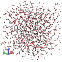
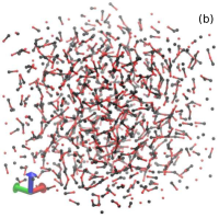
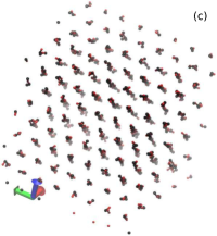
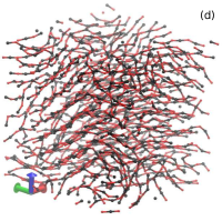
Figure 2: Representative snapshots of the assembled monomers at volume fractions $\phi_{p}$ of (a) $\phi_{p}=0.08$ with short chains and many monomers and dimer (b) $\phi_{p}=0.09$ with larger fraction of long chains (c) $\phi_{p}=0.095$ with long assembled chains parallel to each other with line-hexagonal order (d) $\phi_{p}=0.12$ with long polymers where hexagonal order is destroyed. There are equal number of A and B particles, each of diameter $\sigma$. The A-particles are coloured red and the $B-$ particles are black. The snapshots are for $20\times 20\times 20\sigma^{3}$ box (for easier viewing), corresponding snapshots for a bigger box size of $30\times 30\times 50\sigma^{3}$ are given in Figs S1, S2. In the snapshot (c) the polymer chains are orientationally ordered and are all parallel to each other. The view direction is parallel to the polymer chains and the orientation direction is into the plane of the paper, we choose this to enable the reader to clearly decipher the line-hexagonal order. Plots of same system as seen from other directions are in Supplementary section (Fig. S3).

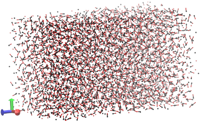
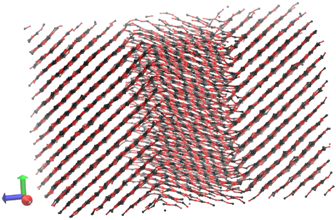
Figure S1: Respresentative snapshots of the self assembled polymers at volume fraction $\phi_{p}=0.08$ (top) and $\phi_{p}=0.102$ (bottom) in box size $30\times 30\times 50\sigma^{3}$. The figure at the bottom shows ordered polymers but there are 2 different domains where the direction or orietnation is different.

In Fig.2, we show equilibrium snapshots of self assembled stuctures at low, medium and high volume fraction $\rho_{p}$ of particles in a box of volume $V_{box}=20\times 20\times 20\sigma^{3}$. Corresponding snapshots for a bigger simulation box, $30\times 30\times 50\sigma^{3}$ are shown in the supplementary section, refer Figs. S1 and S2. The volume fraction $\phi_{p}$ calculated as $(N\pi\sigma^{3})/(6V_{box})$, where $N$ is total number A and B particles. The number of A particles in the box is $N/2$. For volume fractions of $\phi_{p}=0.08$, one observes a large number of unassociated monomers, many dimers, as well as chains with $3$ or more monomers. There are very few side-branches emanating out from a linear polymer chain, we have later quantified the number of branches in the system. The chains become significantly longer at $\phi_{p}=0.09$ and at $\phi_{p}=0.091$ (at $\phi_{p}=0.99$ for the bigger box) they span the length of the simulation box and arrange themselves in a line-hexagonal structure, refer Fig.2(b) and (c), respectively. The polymeric chains start developing branches at volume fraction of $\phi_{p}=0.12$ (Fig.2d) and become a branched gel at even higher densities. Note that any particle feels a repulsive potential from other particles upto a distance of $R_{c}=3\sigma$, and if we use $2\sigma$ as an estimate of the diameter of a soft particle (the repulsive energy of a pair of A-A or A-B particle $\sim k_{B}T$ at $2\sigma$), then then an estimate of the effective volume fractions become $\rho_{eff}=0.64,\,0.72,\,0.76,\,0.96$, respectively. As for any system of soft particles, the volume fraction $\rho$ or $\rho_{eff}$ has to be interpreted with care.

This system of particles behaves like a self-assembling system of equilibrium polymers with suitable length distributions. We plot the chain-length distribution in Figure 3(a), i.e. the number of chains $n_{L}$ with $L$ number of monomers in a chain normalized for a box size of volume $(10\sigma)^{3}$. Since both the number of chains and the length of chains keep fluctuating in the simulation box, we choose not to normalize by the total number of chains in box. But since we show data for two different box sizes, we normalize chain length distribution data by using the factor $(10\sigma)^{3}/V_{box}$; i.e. $n_{L}$ is the number of chains one would find in a volume of $(10\sigma)^{3}$. We show the change in the distribution as we vary the volume fraction $\phi_{p}$ and the temperature $T^{*}$ ($k_{B}=1$). The particles start assembling above a volume fraction $\phi_{p}\sim 0.05$ and thereafter maintain an exponential distribution of chain lengths with increasing $\phi_{p}$, as expected for a worm-like micellar system. With increasing density the length of the longest chains present in the system also increases as can be confirmed from Fig.3(a). Data for $\phi_{p}=0.09$ shows significant finite size effects, as the chains are longer and bigger than half the size of box for $(20\sigma)^{3}$ box.

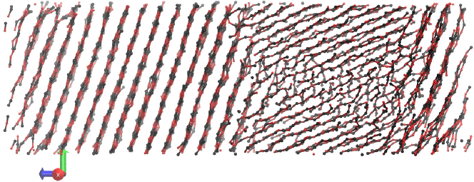
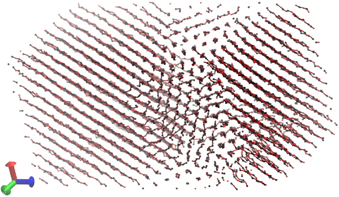
Figure S4: Snapshots of system at $\phi_{p}=0.095$ with boxsizes (a) $20\times 20\times 60$ and (b) $30\times 30\times 60$.

Figure 3(b) shows that the the chains break into smaller assemblies when the temperature $T^{*}$ is increased but the chain length distribution continues to remain linear in a semi-log plot, as expected for self-assembling equilibrium-polymers. In 3(c), we observe that the average length of chains $\langle L\rangle$ gradually increases with $\phi_{p}$, but for $\phi_{p}>0.091$ it shows a jump for a $(20\sigma)^{3}$ box. For the bigger box size of $30\times 30\times 50\sigma^{3}$ box, the jump in $\langle L\rangle$ moves to a slightly higher value of $\phi_{p}$. This happens because the chain arrange themselves in a line-haxagonal order. Simultaneously, they become long enough to span the simulation box to form ring polymers using the periodic boundary condition (PBC) to minimize energy of a polymer chain due to presence of an end-cap. The formation of ring polymers invoking PBC is clearly an artefact of finite size of the simulation box. Snapshots for the self-assembly of particles at $\phi_{p}=0.095$ in different box sizes are presented in the supplementary section (Fig. S4 as well as Fig. S1. From these figures we can conclude that in the thermodynamic limit one can expect the system to form domains of hexagonally ordered chains with different orientation of chains in different domains. An individual long polymer can continue to meander from one domain to the other by suitable bending and looping. It may also possibly form rings (even without invoking PBC). Figure 3(d) shows that the mean length of the self-assembled chains $\langle L\rangle$ increases as $\phi_{p}^{0.5}$ for dilute systems, as predicted by Cates and Candau [23] for worm-like micelles.

To understand the energetics in comparison to thermal energy scales ($k_{B}T$) of the self-assembling systems of polymers we note that at very low densities ($\phi_{p}=0.03$ or $\rho_{eff}=8\phi_{p}$), a pair of bonded A and B monomers gain an average potential energy (PE) per particle of $\approx-2.5k_{B}T$ (refer Fig.1a for graph of potential and Fig.4(a,b) showing PE for two different box sizes); the dashed line represents potential energy (per particle) contribution from bonded A-B interactions. This is offset by the repulsive interactions between particles (A-A,A-B and B-B) which act at larger distances between the particles, such that the total PE combining all attractive and repulsive contributions is nearly zero. But as the density increases the $A-A$ and $B-B$ repulsion starts to play a more significant role than the attractive A-B bond-energy ($\approx-2.5k_{B}T$), the A-A or B-B PE contribution increases and correspondingly the total PE of the system takes increasingly higher positive values, refer Fig. 4a,b. At higher densities, the particles bond to form long polymers (trimers or longer) by using the minima of the potential (refer Fig.1c). Simultaneously we observe that the contribution of the non-bonded (repulsive) A-B interaction becomes nearly zero, as the value of the total PE of A-B interactions is equal that PE contribution due to bonds between A-B particles.

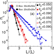
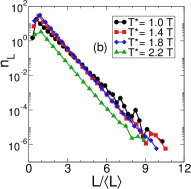
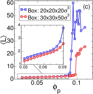
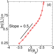
Figure 3: (a) The length distribution of assembled polymeric chains is shown for different volume fractions of monomers. The y-axis shows the average number of chains $n_{L}$ suitably normalized for a box of size $(10\sigma)^{3}$ and the $x$-axis is the length $L$ of the chains, scaled by $\langle L\rangle$: the average length of chain for a particular volume fraction $\phi_{p}$. The number of chains of length $L$ is normalized to the volume of a $(10\sigma)^{3}$ box to obtain $n_{L}$. Thermal energy $k_{B}T=1$. Data for $(20\sigma)^{3}$ is shown with filled symbols; open symbols show data for simulation box $30\times 30\times 50\sigma^{3}$. (b) The length distibution of self-assembled chains at $\phi_{p}=0.09$ at different temperatures $T^{*}/T$ keeping the potential values fixed. (c) The average length of the polymer chains $\langle L\rangle$ with plotted versus the volume fraction of monomers $\phi_{p}$. It shows a jump just above $\phi_{p}=0.091$ in simulation box and at $\phi_{p}=0.099$ in bigger box. The inset shows in detail the data shown in the boxed region of the main graph. (d) The average length $\langle L\rangle$ versus $\phi_{p}$ in a log-log scale to identify the exponent $\alpha$ in $\langle L\rangle\sim\phi_{p}^{\alpha}$.

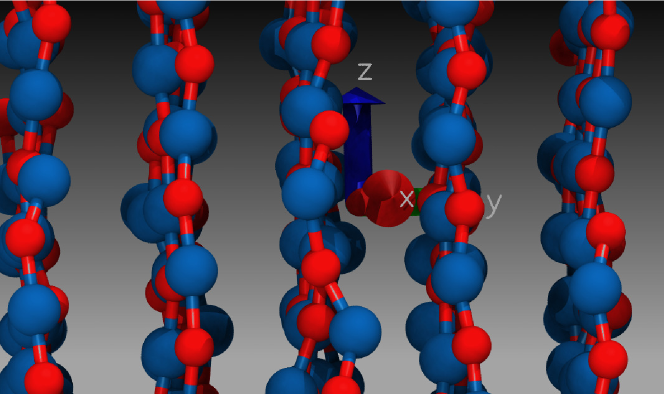
Figure S6: A closer look at chains, which are aligned in the z-direction. One can see that, nearly in all cases, the closest neighbours to an A-particle (red) are B-particles (blue) and vice versa.

For $\phi_{p}>0.09$, the monomers form the line-hexagonal phase and moreover, A and B monomers from adjacent chains adjust their relative positions such that they are nearest each other and A-A (or B-B) repulsive interaction energy between monomers of adjacent chains is minimized. This is clearly seen in the representative snapshot shown supplementary section Fig. S6 and can also be confirmed from the pair correlation function $g(r)$ shown in Fig. 4c. Due to this ordering of chains and re-adjustment of the relative positions of A and B monomers from adjacent chains, we see a drop of total PE of A-B interaction [square symbols in Fig.4(a,b)] near $\phi_{p}=0.091$ ($\phi_{p}=0.099$ for bigger box), however, the mean negative energy (dashed line) contribution from intra-chain bonded $A-B$ monomers remains nearly unchanged across this transition. The total PE of the system shows a discontinuity near $\phi_{p}=0.093$, indicating a first order transition to a orientationally ordered state. The result is robust, the jump in total PE is seen in both the box sizes, only the corresponding $\phi_{p}$ value changes slightly as one changes the box size which is likely to be a finite size effect.

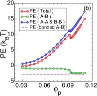
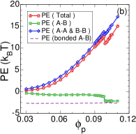
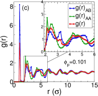
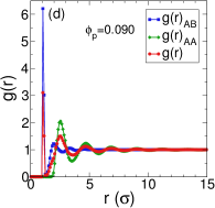
Figure 4: Plots of energy contribution from different pair interaction of A and B monomers for box sizes of (a) $(20\sigma)^{3}$ and (b) $30\times 30\times 50\sigma^{3}$ Different symbols indicate the total PE, PE due to A-B interactions (sum of attractive and repulsive interactions), sum of purely repulsive A-A & B-B interactions, and attractive ponetial energy between A-B which are at distances $r<1.3\sigma$ such that they are bonded. The average potential energy $PE$ in units of $k_{B}T$ of the system versus $\phi_{p}$ show a discontinuity at the same $\phi_{p}$ where $\langle L\rangle$ shows the jump. Pair correlation functions $g(r)$ at volume fractions (c) $\phi_{p}=0.09$ and (d) $\phi_{p}=0.101$ [line-hexagonal phase] for box size $30\times 30\times 50\sigma^{3}$ for all monomers, A-A/B-B pair of monomers and A-B monomer pairs.

We calculate the pair correlation function $g(r)$ between monomers, the $g(r)$ data is shown in Figs.4(c,d). When the monomers form domains of parallel polymers ordered in line-hexagonal phase at $\phi_{p}=0.10$ for the bigger boxsize, the first peak of $g(r)_{AB}$ between A and B monomers shows up at a distance just beyond $1\sigma$ corresponding to the distance between adjacent A and B bonded monomers in a chain. The next peak in $g(r)_{AB}$ at distance just beyond $2\sigma$ is due to the arrangment between A and B monomers from adjacent chains, as discussed in the previous paragraph. The third peak just beyond a distance of $3\sigma$ is a consequence of the arrangement of monomers belonging to the same chain: the second nearest neighbour A-monomer from a B-monomer along a chain will be at a distance of about $3\sigma$. The $g(r)_{AA}$, the pair correlation fucntion between A-monomers (equivalently B monomers) shows the first peak at $2\sigma$ corresponding to the smallest distance between A-monomers along the contour length of a self-assembled chain. The two A-monomers have a B-monomers in between them. The next peak corresponds to A-monomers from adjacent chain. The quantity $g(r)$ is the pair correlation function between all monomers without discriminating between A and B monomers, it shows the peaks of both $g(r)_{AA}$ and $g(r)_{AB}$. The total $g(r)$ shows regular peaks upto half the length of the box, which corresponds to long-range ordering of chains and thereby monomer positions. In contrast $g(r)$ for lower volume fractions (e.g. $\phi_{p}=0.09$, refer Figs.4(d) shows the first two peaks for $g(r)_{AA}$ and $g(r)_{BB}$ but there is no long range order to be seen.

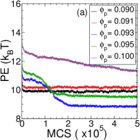
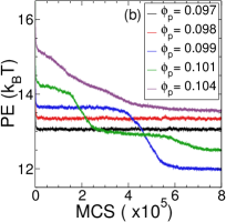
Figure 5: The total potential energy (PE) vs number of Monte Carlo steps (MCS) for different values of $\phi_{p}$ for box sizes (a) $(20\sigma)^{3}$ and (b) $30\times 30\times 50\sigma^{3}$ to check the approach to equilibrium of the different systems.

Figures 5(a,b) show the potential energy $PE$ of the system plotted every $100$ Monte Carlo steps (MCS) for different values of $\phi_{p}$ to enable us to analyze the approach to equilibrium of the self-assembled chains, especially when domains with line-hexagonal phases are formed. For relatively lower values $\phi_{p}$ ($\phi_{p}=0.09$), the system reaches equilibrium within $0.2\times 10^{5}$ MCS for the box size of $(20\sigma)^{3}$ starting from a random initial configuration of monomers and then the energy fluctuates about the average value of energy. But for $\phi_{p}=0.093$ and $\phi_{p}=0.095$, the energy first shows a small plateau till around $1\times 10^{5}$ MCS (for small box), and then settles down to a lower mean value of PE after $2\times 10^{5}$ MCS. The mutual repulsion between self-assembled chains arising from the repulsion between A-A and A-B particles (for $r>1.3\sigma$) keeps the polymer chains straight and parallel to each other.

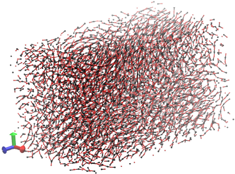
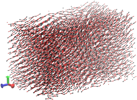
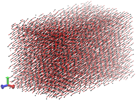
Figure S5: Snapshots of system at different simulation times for $\phi_{p}=0.101$. The top panel is at $1.6\times 10^{5}$ MCS after the beginning of the run, the middle panel is at $2.4\times 10^{5}$ MCS and the bottom is at $10\times 10^{5}$ MCS. Data is for bigger box size.

We see similar relaxation behaviour at $\phi_{p}=0.099$ and $\phi_{p}=0.101$ for simulations in the bigger box size where there are steps in PE in at $2\times 10^{5}$ and $4\times 10^{5}$ MCS, respectively; longer relaxation times for bigger box sizes are expected. For the runs with $\phi_{p}=0.101$, snapshots of the configuration before $2\times 10^{5}$ MCS, between $2\times 10^{5}$ and $6\times 10^{5}$ MCS, and after $6\times 10^{5}$ MCS are shown in the supplementary section for the bigger box size (Fig. S5). After the initial transient relaxation (at $0.1\times 10^{5}$ MCS) long self-assembled chains are formed from the monomers till $2\times 10^{5}$ MCS, but after the PE dip at $2\times 10^{5}$ MCS, the polymers spontaneously self-organize themselves into small domains with hexagonal line order. After $6\times 10^{5}$ iterations, the small domains reorganize into much larger domains, and one sees a corresponding second dip in the energy plot of 5(b) for $\phi_{p}=0.101$. At densities of $\phi_{p}=0.1$ (or more), the system has not equilibrated within the simulation time scales, but we do not present statiscally averaged quantities for the high density regime.

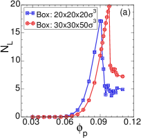
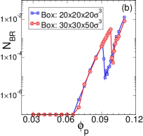
Figure 6: (a) The average number $N_{L}$ of self-assembled chains in a volume of $(10\sigma)^{3}$ ( obtained from simulations box sizes of $(20\sigma^{3})$ and $30\times 30\times 50\sigma^{3}$) is plotted versus the volume fraction of monomers $\phi_{p}$. $N_{L}$ counts only those chains which number of monomers $L>3$ in a chain. (b) The plots shows the average number of branches $N_{BR}$ (suitably normalized for a box of size of $(10\sigma)^{3}$ as before) plotted against the monomer volume fraction $\phi_{p}$. Branched configurations need to have a minimum of $4$ or more monomers in a chain. The values shown as $N_{BR}<10^{-6}$ are actually zero, they have been by hand set to $10^{-7}$ to enable us to show them in a log-scale in the figure.

Figure 6(a) shows that the number of chains $N_{L}$ with $L>3$ in simulation box, normalized by the volume of a $(10\sigma)^{3}$ simulation box (normalization reason discussed previously, refer text of Fig. 3), though we present data for simulations performed in $30\times 30\times 50\sigma^{3}$ box, and in $(20\sigma)^{3}$ box sizes. There are very few chains with length $L>3$ for $\phi_{p}<0.06$; however, $N_{L}$ increases with $\phi_{p}$ for $\phi_{p}>0.06$. For $\phi_{p}>0.091$, the chains straighten and become parallel to each other to form the line-hexagonal phase, and the number of chains drops and remains nearly fixed at the number of parallel chains accommodated in the system. The chain length distribution is no longer exponential, and large fluctuations are seen in the value of $N_{L}$ when chains break. In a square cross section of $(10\sigma)^{2}$, there are around $7$ to $9$ chains with area fraction of $8\pi r^{2}/(10\sigma)^{2}=0.36$ considering $r=1.2\sigma$ calculated from the second peak of $g_{AB}(r)$ data. Furthermore, $\langle L\rangle$ is of the same order as the largest dimension of the box ($20\sigma$ or $50\sigma$). Hence the numbers for $\langle L\rangle$ for $\phi_{p}>0.09$ can be expected to have strong finite size effects. Fig.6(b) shows that the average number of branches in a particular microstate (snapshot) in the system is very small, compared to the number of chains $N_{L}(L>3)$ in the system. The number of branches increases as we change $\phi_{p}$ from $0.06$ to $0.09$, but still remains insignificant compared to the number of chains $n_{L}(L>3)$ in the system. Since the number of branches per chain always has such a very low value, effectively there are no branches in our system for $\phi_{p}<0.09$.

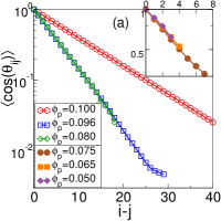
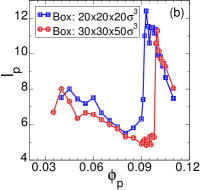
Figure 7: (a) The mean of the cosine of the angle $\theta_{ij}$ between two bond vectors $\vec{b_{i}}$ and $\vec{b_{j}}$ along the length of the chain as a function of the index $i-j$, where $i$ and $j$ are the bond vector indices along the contour length of the chain. The number of bonds in a chain with $L$ monomers $L-1$. At low densities, since the self assembled chains are very short the maximum value of $i-j$ is relatively low and the data is shown in the inset. The data from $30\times 30\times 50\sigma^{3}$ box size has been plotted in a semi-log plot to extract $l_{p}$ by using $\langle\cos(\theta_{ij})\rangle\sim e^{-(i-j)\sigma/l_{p}}$. (b) The persistence length $l_{p}$ versus the volume fraction $\phi_{p}$ of monomers have been shown for both box sizes. The standard deviation calculated for the data for smaller box is obtained from 10 independent runs.

The tendency of the chains to line up parallel to each other at high densities ($\phi_{p}>0.09$) also brings up the question of how semiflexible the chains are, and we quantify semiflexibily by calculating the persistence length $l_{p}$ of the polymer chains as function of $\phi_{p}$. To calculate $\ell_{p}$, all chains with more than $3$ monomers are identified, and bond vectors $\vec{b_{i}}$ joining adjacent monomers along the chain contour are calculated. A chain with $L$ monomers will have $i$ running from $1$ to $L-1$. Then the quantity $\langle\cos(\theta_{ij})\rangle=\langle\vec{b_{j}}\cdot\vec{b_{i}}\rangle$ is calculated for all values of $i-j$, where $i-j=1,2..,(L-2)$. The plot of $\langle\cos(\theta_{ij})\rangle$ versus $i-j$ is shown in Fig.7(a) for different values of $\phi_{p}$ in a semilog plot. We do a exponential fit to calculate the values of the peristence length $l_{p}(\phi_{p})$ for each $\phi_{p}$, refer Fig.7(b). The $l_{p}(\phi_{p})$ (effective persistence length) shows a jump at $\phi_{p}=0.09$ as the chain get into the line-hexagonal ordered state, below that the $l_{p}$ is around 6 bond-lengths. Below $\phi_{p}<0.09$, the decrease of $l_{p}$ with increasing $\phi_{p}$ could be due to the effect of self avoidance of many chains trying to fit with each other in the box. Persistence length $l_{p}$ is a single chain property and should ideally be calculated at low densities of monomers. But at low densities of monomers, longer chains of self-assembling monomers are relatively rare and values of $l_{p}$ around $\phi_{p}=0.05$ and $\phi_{p}=0.065$ should be considered reliable.

Such a simple model for self-assembled polymers can be used to study a range of properties of worm-like micellar systems only if one can tune $l_{p}$ and branching of the chains. The persistence length $l_{p}$ is a single chain property and should be calculate for dilute systems. To that end, we changed parameters of the repulsive potential $V_{AA}(r)=V_{BB}(r)$.

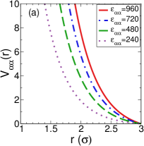
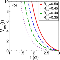
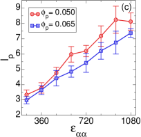
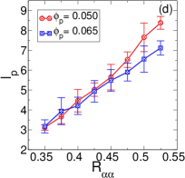
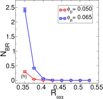
Figure 8: Subplots (a) and (b) show the change in potential of interaction between like particles $V_{\alpha\alpha}\,\,(V_{AA},V_{BB})$ on changing parameters $\epsilon_{\alpha\alpha}$ (in units of $k_{B}T$) or $R_{\alpha\alpha}$ (in units of $\sigma$). Both $V_{AA}$ and $V_{BB}$ are changed simultaneously when we change the parameters. Subplots (c) and (d) show corresponding changes in the persistence length $l_{p}$ (solid symbols) and (e) and (f) show the number of branches (open symbols), normalized for a $(10\sigma)^{3}$ box at two relatively low volume fractions $\phi_{p}$ of monomers.

We change either the strength of the repulsive potential ($\epsilon_{\alpha\alpha}$) between like monomers keeping $R_{AA},R_{BB}$ constant. Alternatively, we change the range of interactions ($R_{AA}$ and $R_{BB}$), keeping $\epsilon_{\alpha\alpha}$ fixed, refer Fig.8(a,b). We then investigate the corresponding change in the values of $l_{p}$ and $N_{br}$ on change of the above parameters. As one changes the parameters such that the range of the repulsive potential decreases, the value of the persistence length decreases from the values of $\approx 8.5\sigma$ to lower values as seen in Figs.8(c,d). For these calculations we choose relatively lower values of $\phi_{p}=0.05$ or $\phi_{p}=0.06$ for reasons discussed previously. The drop in values of $l_{p}$ occurs because decrease in $V_{AA}$ (and $V_{BB}$) potential allows two A particles in a A-B-A configuration to approach each other. Consequently, increasing the repulsion between like-particles will keep $A-B-A$ configuration in straight line and increase $l_{p}$. Furthermore, there is a corresponding significant increase in branching with decrease in the repulsive potential between like-particles, refer Figs.8(e,f) This is because lowering the repulsion between $A-A$ (or $B-B$) particles allows a fourth particle (say) A to approach a (say) $-A-B-A-$ configuration by getting closer to (say) B in the triplet. Note that, the increase in $l_{p}$ is nearly the same on decrease of either $R_{\alpha\alpha}$ or $\epsilon_{\alpha\alpha}$ as the relative decrease in the values of $V_{\alpha\alpha}$ is nearly the same for the range of parameters considered.

IV Conclusions

Spherically symmetric potentials with short range attraction and long range repulsion have been suggested and used by previous studies [15, 16, 17, 18] but they obtained linear cluster of particles, or polymers with branches with additional three-body term to incorporate semi-flexibility. There are two crucial ideas which led to our success in obtaining linear polymeric chains without branching using same class of potentials. Firstly, we used $(1/r)^{24}-(1/r)^{12}$ instead of Lennard Jones term which led to a sharper minima of the attractive part of the potential. This enabled us to have a sharp potential peak at rather short distances near $r=1.3\sigma$. In the past we have tried to get a sharp peak at such distances with Lennard Jones potential but without success [6, 40]. Secondly, we used 2 kinds of particles A and B. The repulsion between like particles control the persistence length and reduce the probability of branching. There have been previous studies which have obtained assemblies of particles with linear and other anisotropic morphologies [1] starting out with isotropic potentials, but they have used 4 (or more) different kind of particles. Our proposed model is much simpler. and could be experimentally realizable with spherical charged colloidal particles with tunable attractive potential [41, 42, 43, 44, 45] and screened Coulomb repulsions to form polymeric chains.

We acknowledge funding and the use of a cluster bought using DST-SERB grant no. EMR/2015/000018 to A. Chatterji. AC acknowledges funding support by DST Nanomission, India under the Thematic Unit Program (grant no.: SR/NM/TP-13/2016) and DBT project BT/PR16542/BID/7/654/2016. AC acknowledges Rahul Pandit (IISc, Bangalore) who proposed this problem 20 years ago.

Chapter Supplementary Materials

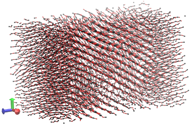
Figure S2: Respresentative snapshots of the self assembled polymers at volume fraction $\phi_{p}=0.11$ in box size $30\times 30\times 50\sigma^{3}$. One observes that as we increase density to $\phi_{p}=0.11$, there is a domain of ordered polymers (line hexagonal order) but in the other region the organization of chains is lost: the chains look disordered.

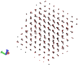
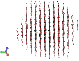
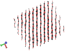
Figure S3: Snapshots of system at $\phi_{p}=0.095$ with boxsize $20\times 20\times 20$, viewed from different directions, as it is continuously rotated to enable to reader to deciper the inter-chain and inter-particle ordering.

References

- Gruenwald and Geissler [2014] M. Gruenwald and P. L. Geissler, ACS Nano 8, 5891 (2014).
- Jacobs and Frenkel [2015] W. M. Jacobs and D. Frenkel, Soft Matter 11, 8930 (2015).
- Reinhardt and Frenkel [2014] A. Reinhardt and D. Frenkel, Phys. Rev. Lett. 112, 238103 (2014).
- Barros and Luijten [2014] K. Barros and E. Luijten, Phys. Rev. Lett. 113, 017801 (2014).
- Kegel and van der Schoot [2004] W. K. Kegel and P. van der Schoot, Biophysical Journal 86, 3905 (2004).
- Mubeena and Chatterji [2015] S. Mubeena and A. Chatterji, Phys. Rev. E 91, 032602 (2015).
- Grason [2016] G. M. Grason, The Journal of Chemical Physics 145, 110901 (2016).
- McManus et al. [2016] J. J. McManus, P. Charbonneau, E. Zaccarelli, and N. Asherie, “The physics of protein self-assembly,” (2016), arXiv:1602.00884v1 [cond-mat.soft] .
- Angioletti-Uberti et al. [2016] S. Angioletti-Uberti, B. M. Mognetti, and D. Frenkel, Phys. Chem. Chem. Phys. 18, 6373 (2016).
- Bruinsma et al. [2016] R. F. Bruinsma, M. Comas-Garcia, R. F. Garmann, and A. Y. Grosberg, Phys. Rev. E 93, 032405 (2016).
- Theodorakis et al. [2015] P. E. Theodorakis, N. G. Fytas, G. Kahl, and C. Dellago, “Self-assembly of dna-functionalized colloids,” (2015), arXiv:1503.05384 [cond-mat.soft] .
- Whitelam and Jack [2015] S. Whitelam and R. L. Jack, Annual Review of Physical Chemistry 66, 143 (2015).
- Glotzer and Solomon [2007] S. C. Glotzer and M. J. Solomon, Nature Materials 6, 557 (2007).
- Akcora et al. [2009] P. Akcora, H. Liu, S. K. Kumar, J. Moll, Y. Li, B. C. Benicewicz, L. S. Schadler, D. Acehan, A. Z. Panagiotopoulos, V. Pryamitsyn, V. Ganesan, J. Ilavsky, P. Thiyagarajan, R. H. Colby, and J. F. Douglas, Nature Materials 8, 354 (2009).
- Mossa et al. [2004] S. Mossa, F. Sciortino, P. Tartaglia, and E. Zaccarelli, Langmuir 20, 10756 (2004).
- Sciortino et al. [2004] F. Sciortino, S. Mossa, E. Zaccarelli, and P. Tartaglia, Phys. Rev. Lett. 93, 055701 (2004).
- Das et al. [2017] S. Das, J. Riest, R. G. Winkler, G. Gompper, J. K. G. Dhont, and G. Naegele, Soft Matter , (2017).
- Chen et al. [2011] J.-X. Chen, J.-W. Mao, S. Thakur, J.-R. Xu, and F.-y. Liu, The Journal of Chemical Physics 135, 094504 (2011).
- Vliegenthart et al. [1999] G. Vliegenthart, J. Lodge, and H. Lekkerkerker, Physica A: Statistical Mechanics and its Applications 263, 378 (1999), Proceedings of the 20th IUPAP International Conference on Statistical Physics.
- Berret [2004] J.-F. Berret, “Rheology of wormlike micelles : Equilibrium properties and shear banding transition,” (2004), eprint arXiv:cond-mat/0406681 .
- Dreiss [2007] C. A. Dreiss, Soft Matter 3, 956 (2007).
- Dreiss [2017] C. A. Dreiss, in Wormlike Micelles: Advances in Systems, Characterisation and Applications (The Royal Society of Chemistry, 2017) pp. 1–8.
- Cates and Candau [1990] M. E. Cates and S. J. Candau, Journal of Physics: Condensed Matter 2, 6869 (1990).
- Milchev and Landau [1995] A. Milchev and D. P. Landau, Phys. Rev. E 52, 6431 (1995).
- Huang et al. [2006] C. Huang, H. Xu, and J.-P. Ryckaert, The Journal of Chemical Physics 125, 094901 (2006).
- Huang et al. [2008] C.-C. Huang, H. Xu, and J. P. Ryckaert, EPL (Europhysics Letters) 81, 58002 (2008).
- Huang et al. [2009] C.-C. Huang, J.-P. Ryckaert, and H. Xu, Phys. Rev. E 79, 041501 (2009).
- Padding et al. [2009] J. T. Padding, W. J. Briels, M. R. Stukan, and E. S. Boek, Soft Matter 5, 4367 (2009).
- Padding and Boek [2004a] J. T. Padding and E. S. Boek, EPL (Europhysics Letters) 66, 756 (2004a).
- Padding and Boek [2004b] J. T. Padding and E. S. Boek, Phys. Rev. E 70, 031502 (2004b).
- Padding et al. [2005] J. T. Padding, E. S. Boek, and W. J. Briels, Journal of Physics: Condensed Matter 17, S3347 (2005).
- Chatterji and Pandit [2001] A. Chatterji and R. Pandit, EPL (Europhysics Letters) 54, 213 (2001).
- Thakur et al. [2010] S. Thakur, K. R. Prathyusha, A. P. Deshpande, M. Laradji, and P. B. S. Kumar, Soft Matter 6, 489 (2010).
- Prathyusha et al. [2013] K. R. Prathyusha, A. P. Deshpande, M. Laradji, and P. B. Sunil Kumar, Soft Matter 9, 9983 (2013).
- Bandyopadhyay et al. [2000] R. Bandyopadhyay, G. Basappa, and A. K. Sood, Phys. Rev. Lett. 84, 2022 (2000).
- Bandyopadhyay and Sood [2001] R. Bandyopadhyay and A. K. Sood, EPL (Europhysics Letters) 56, 447 (2001).
- Ganapathy et al. [2008] R. Ganapathy, S. Majumdar, and A. K. Sood, Phys. Rev. E 78, 021504 (2008).
- Das et al. [2005] M. Das, B. Chakrabarti, C. Dasgupta, S. Ramaswamy, and A. K. Sood, Phys. Rev. E 71, 021707 (2005).
- Angioletti-Uberti et al. [2014] S. Angioletti-Uberti, P. Varilly, B. M. Mognetti, and D. Frenkel, Phys. Rev. Lett. 113, 128303 (2014).
- Abraham [2016] A. Abraham, “Self-assembly of polymeric chains under a new radially symmetric potential,” MS Thesis (2016).
- Binder et al. [2014] K. Binder, P. Virnau, and A. Statt, The Journal of Chemical Physics 141, 140901 (2014).
- Zausch et al. [2009] J. Zausch, P. Virnau, K. Binder, J. Horbach, and R. L. Vink, The Journal of Chemical Physics 130, 064906 (2009).
- Biben et al. [1996] T. Biben, P. Bladon, and D. Frenkel, Journal of Physics: Condensed Matter 8, 10799 (1996).
- Crocker et al. [1999] J. C. Crocker, J. A. Matteo, A. D. Dinsmore, and A. G. Yodh, Phys. Rev. Lett. 82, 4352 (1999).
- Yethiraj [2007] A. Yethiraj, Soft Matter 3, 1099 (2007).
Chapter \thechapter Supplementary Materials