Quadrilateral grid generation supported on complex internal boundaries using spectral methods

Abstract

This work concerns with the following problem. Given a two-dimensional domain whose boundary is a closed polygonal line with internal boundaries defined also by polygonal lines, it is required to generate a grid consisting only of quadrilaterals with the following features: (1) conformal, that is, to be a tessellation of the two-dimensional domain such that the intersection of any two quadrilaterals is a vertex, an edge or empty (never a portion of one edge), (2) structured, which means that only four quadrilaterals meet at a single node and the quadrilaterals that make up the grid need not to be rectangular, and (3) the mesh generated must be supported on the internal boundaries. The fundamental technique for generating such grids, is the deformation of an initial Cartesian grid and the subsequent alignment with the internal boundaries. This is accomplished through the numerical solution of an elliptic partial differential equation based on finite differences. The large nonlinear system of equation arising from this formulation is solved through spectral gradient techniques. Examples of typical structures corresponding to a two-dimensional, areal hydrocarbon reservoir are presented.

1 Introduction

Nowadays the crude oil is not only one of the world’s most important combustibles but also it becomes almost half of the energy consumption in the world. For these reasons, it is important to take care and to correctly administrate the earth’s existing oil reserves. Also, the ability to predict the performance of a petroleum reservoir is of immense importance for the petroleum industry.

A petroleum reservoir is the place where oil stores naturally. Every reservoir is unique based on its geological or geophysical characteristics, and the type of crude oil the formation contains. Wells are drilled into oil reservoirs to extract the crude oil. All this makes the oil extraction and exploitation methods to be very costly.

For obvious reasons it is very useful to predict the behavior of the reservoir before and during its exploitation. One would like to be able to know as much as possible about production rates and total production resulting from different production strategies.

The petroleum engineer needs to understand at least, the complex reservoir structure and the fluid movement through it, to generate an exploitation plan in order to make the right predictions of the reservoir production.

At this point, it is where the numerical reservoir simulators play an important role in the reservoir exploitation. To this end, numerical reservoir simulation has gained wide acceptance as an important decision-making tool, and has become the industry standard for reservoir management.

By numerical reservoir simulation we mean the process of inferring the behavior of a real reservoir from the performance of a mathematical model of that physical system. Traditionally, the petroleum engineer represents mathematically an oil reservoir through its discrete model using rectangular meshes, in order to perform numerical reservoir simulations to predict the oil production in time. However, the geological structure of the oil reservoir is not adequately represented using rectangular meshes. The discrete model of the reservoir must honor the natural boundaries of the reservoir (see [7]). Given today’s reality, the petroleum engineer should align the grid, for instance, with the principal directions of deposition and to the preferential flow directions. A grid (the discrete model) that adequately represents a hydrocarbon reservoir is fundamental to be used with any mathematical model that allows to calculate the total amount of oil that will ever be recovered according to probable scenarios. For example, when or where to drill additional producer wells, injector wells, when to shut in wells, to inject water or gas, or to prove other techniques for increasing the amount of crude oil that can be extracted from an oil field.

For our purposes, the mathematical model is a set of partial differential equations with an appropriate set of boundary conditions, which describes the significant physical processes taking place in the system (the reservoir).

The mathematical modeling of the multi-phase fluid flow in a porous media then requires grids that represent the complexity of the reservoir structure. On this relay the interest of generating certain types of grids that honor the reservoir structure through their alignment to a set of internal boundaries. There are two types of grids, structured or unstructured, that can solve this problem. A structured mesh can be recognized by all interior nodes of the mesh having an equal number of incidence elements. Unstructured mesh generator, on the other hand, relaxes the node valence requirement, allowing any number of elements to meet at a single node.

A lot of studies concerning grid generation have been conducted under structured/unstructured and/or orthogonal/non-orthogonal grids using finite elements and finite differences. Various shaped meshes are widely introduced, such as tetrahedral or hexahedral meshes under non-orthogonal or unstructured mesh system, which are very suitable for fitting complex geometry.

This work will be confined to structured meshes in two-dimensional domains corresponding to areal (2D) or transversal views of oil reservoirs. From this type of grids, a three dimensional mesh can be generated: starting from a two dimensional grid on a reference plane, sweep it through space along a curve between a source and target surface. The source and target surface correspond to layers of the 3D domain (the reservoir). It is sometimes referred to as 2$\frac{1}{2}$D meshing.

The rectangular meshes are inappropriate to model any type of internal boundaries. For example, in case of internal boundaries forming different angles with the coordinate axes, a rectangular mesh will give stairs shaped paths to model the boundaries, which could distort the flow field in the vicinity of that boundary. That is why the interest of this work will be concentrated on quadrilateral meshes.

In summary, given a rectangular domain, the reservoir, this work is concerned with the generation of a 2D non orthogonal structured grid consisting only of quadrilaterals that honor the internal boundaries of the domain.

Some publications related to the goal of the present work will be detailed next.

Winslow (1966) in [29] proposed a method to generate a triangular mesh by solving Laplace s equation. The method can be derived by formulating the zoning problem as a potential problem, with the mesh lines playing the role of equipotentials. Because of the well-known averaging property of solutions to system of Laplace equations, we might expect a mesh constructed in this way to be, in some sense, smooth. Winslow said this methodology is easily adapted to non rectangular boundaries and interfaces.

Amsden and Hirt (1973) in [1] proposed an iterative process to transform a rectangular grid into a more complex configuration, by the direct solution of a Laplace equation type. The final grid is made of quadrilateral elements only. Even though the domain does not have internal boundaries, the methodology has the potential to handle such type of constrains.

Thompson et al. (1974) in [23, 24] extended the works in [29] and [1] to generate quadrilateral meshes as solutions of an elliptic differential system to multiconnected regions with any number of arbitrary shape bodies or holes. Their work was confined to two dimensions in the interest of compute economy, but all techniques are immediately extendable to three dimensions.

Knupp (1992) in [12] proposed a variational principle that results in a robust elliptic grid generator having many of the strengths of [29] and [1, 24]. This grid generator places grid lines more uniformly over the domain without loss of orthogonality. Grid quality measures were introduced to quantify differences between discrete grids. The author states that generalization of the new method to surface and volume grid generation is straightforward.

Borouchaki and Frey (1996 and 1998) in [3, 4] proposed a method to generate quasi quadrilateral meshes based on an automatic triangular to quadrilateral mesh conversion scheme. This method allows refining the mesh in order to capture the behavior of the underlying physical phenomenon, but the resulting mesh is not entirely composed by quadrilaterals. The main contribution is to extend the triangle merging procedure to the case where a generalized metric map is specified. They also introduced a new mesh optimization technique based on vertex smoothing.

Sarrate and Huerta (2000) in [21] described an algorithm for automatic unstructured quadrilateral mesh generation based on a recursive decomposition of the domain into quadrilateral elements. Two facts for the generated mesh can be highlighted: (1) there is no need for a previous step where triangles are generated, and (2) the generated quadrilateral mesh may have more or less than four elements meeting at a single node. The model is applied to complex geometry domains without internal boundaries.

Hyman et al. (2000) in [9] presented a numerical algorithm that aligns a structured quadrilateral grid with internal alignment curves. These curves represent internal boundaries that can be used to delineate internal interfaces, discontinuities in material properties, internal boundaries, or major features of a flow field. The authors use Gauss-Seidel iterations to solve the Thompson, Thames and Mastin (TTM) smoothing equations (see [23, 24]). The smoothing regularizes the distribution of the grid points, is guaranteed to converge, and eliminates overlapping grid cells. The Gauss-Seidel iterations are halted when the residual of the TTM equations falls below a small tolerance. For complex internal boundaries the authors admit that is extremely difficult to automate the procedure.

Sarrate and Huerta (2002) in [22] presented the extension of the unstructurated and quadrilateral grid generation algorithm in [21] to three dimensional parametric surfaces. The target of this extension is to build the discretization in the plane of parameters and then map the obtained mesh on the surface according to its geometric properties.

Kyu-Yeul et al. (2003) in [14] proposed an algorithm, based on the constrained Delaunay triangulation and Q-Morph algorithm, to automatically generate a 2D unstructured quadrilateral mesh which handles line constraints. The triangulation method is the one who handle line constraints. Q-Morph utilizes an advancing front approach to combine triangles into quadrilaterals. Kyu-Yeul et al. implemented the constrained Laplacian smoothing method to improve mesh quality. This methodology does not involve the resolution of any nonlinear system.

Lin et al. (2007) in [15] presented a Bézier patch mapping algorithm, based on a bijective boundary-conforming mapping method, which generates a strictly non-self-overlapping structured quadrilateral grid in a given four-sized planar region, whose boundaries are polynomial curves. Finally, a constrained optimization problem is formualted in order to ensure the bijectiveness of Bézier patch mapping. This problem is solved using the Matlab optimization library. This methodology does not handle any type of domain internal boundaries.

Parka et al. (2007) in [17] developed an automated method of quadrilateral mesh with random line constraints. The algorithm is based on advanced front techniques and a direct method to handle line-typed features automatically without any user interactions and modification. The generated mesh does not require a previous triangular mesh, and in general it is not structured.

Villamizar et al. (2007 and 2009) in [28, 27] proposed a 2D elliptic grid generator to create a structured quadrilateral smooth mesh with boundary conforming coordinates and grid lines control, on multiply connected regions including boundary singularities. The generator is based on numerical solution of a Poisson equations system and the grid line spacing is controlled by a specific nodal distribution on appropriated boundary curves. This technique does not take into account any type of internal boundaries.

Berndt et al. (2008) in [2] presented two Jacobian-Free Newtown-Krylov (JFNK) solvers for Laplace-Beltrami grid generation system of equations. The two JFNK solvers differ only in the preconditioner. A key feature of these methods is that the Jacobian is not formed explicitly.

Ruiz-Gironés and Sarrate (2008 and 2010) in [19, 20] proposed a modification of the submapping method to generate structured quadrilateral meshes, in order to be applied to geometries in which the angle between two consecutive edges of its boundary is not an integer multiple of $\pi/2$. The submapping method splits the geometry into pieces logically equivalent to a quadrilateral, and then, meshes each piece keeping the mesh compatibility between them by solving an integer linear problem. They used the transfinite interpolation method (TFI) to mesh each patch. In addition, the authors proposed a procedure to apply it to multiply connected domains. Also, they present several numerical examples that show the applicability of the developed algorithms.

Khattri (2009) in [10] presented the elliptic grid generation system for generating adaptive quadrilateral meshes, and its implementation in the C++ language. The coupled elliptic system are linearised by the method of finite differences, and the resulting system is solved by the SOR relaxation. The presented method generates adaptive meshes without destroying the structured nature of the mesh. This technique does not take into account any type of internal boundaries.

Evasi-Yadecuri and Mahani (2009) in [7] presented a novel unstructured (coarse) grid generation approach using structured background grid. A structured/cartesian fine grid distribution of properties, either static or dynamic, is utilized to create background grid or spacing parameter map. Once background grid is generated, advancing front triangulation and then Delaunay tessellation are invoked to form the final (coarse) gridblocks. This technique does not take into account any type of internal boundaries.

Liu et al. (2011) in [16] presented an indirect approach for automatic generation of unstructured quadrilateral mesh with arbitrary line constraints. The methodology follows the steps: (1) discretizing the constrained lines within the domain; (2) converting the above domain to a triangular mesh together with the line constraints; (3) transforming the generated triangular mesh with line constraints to an all-quad mesh through performing an advancing front algorithm from the line constraints, which enables the construction of quadrilaterals layer by layer, and roughly keeps the feature of the initial triangular mesh; (4) optimizing the topology of the quadrilateral mesh to reduce the number of irregular nodes; (5) smoothing the generated mesh toward high-quality all-quad mesh generation.

Rathod et al. (2014) in [18] described a scheme for unstructured quadrilateral mesh generation of a convex, non-convex polygon and multiple connected linear polygon. They decompose these polygons into simple sub regions in the shape of triangles. These simple regions are then triangulated to generate a fine mesh of triangular elements. Finaly, the authors proposed an automatic triangular to quadrilateral conversion scheme. Although the paper describes the scheme as applied to planar domains, the author states that it could be extended to 3D.

Fortunato et al. (2016) in [8] proposed the generation of unstructured high-order meshes by solving the classical Winslow equations. They described a new continuous Galerkin finite element formulation of the standard Winslow equations, which they use for generation of well-shaped high-order unstructured curved meshes. Compared to other finite element formulations in the literature, their discretization attempts to directly mimic the non-conservative form used by most finite difference solvers, which allows for a highly efficient Picard solver.

The methodology proposed in the present work follows the technique proposed by Hyman et al. (2000) in [9], also see [5] and [26], to generate grids that represent the complexity of the reservoir structure, because it does not require a previous triangular mesh, the resulting quadrilateral mesh is well adapted to internal boundaries and is structured and non necessarily orthogonal. The generation of such grid is accomplished through the numerical solution of a system of elliptic partial differential equation (see [25] and [10]) based on finite differences. The large nonlinear system arising from this discretization are solved using spectral gradient techniques (see [13]), which are low in storage and low in computational cost. Buitrago et al. (2015) in [6], proposed a numerical model based on finite volume methods for the solution of the 2D convection diffusion equation on the type of meshes presented in this work, i.e. non-rectangular grids formed only by quadrilaterals honouring the internal structures of the domain.

2 Formulation of the problem

This work concerns with the following problem.

Given a two-dimensional domain $\Omega$ whose external boundary is a closed polygonal line with internal boundaries defined also by polygonal lines, it is required to generate a grid consisting only of quadrilaterals with the following features:

1. conformal, that is, to be a tessellation of the two-dimensional domain $\Omega$ such that the intersection of any two quadrilaterals is a vertex, an edge or empty (never a portion of one edge),

2. structured, but non cartesian, this means that the quadrilaterals that make up the grid need not to be rectangular and only four quadrilaterals meet at a single node, and

3. the mesh generated must be supported on the internal boundaries.

It is also considered the possibility that interior points in $\Omega$ be vertices of the resulting grid. These points will represent wells on the reservoir to simulate. Internal boundaries, that may have a complex layout and configuration, mimic the structure of the reservoir.

The fundamental technique for generating such type of grids, is the deformation of an initial Cartesian grid and the subsequent alignment with the internal boundaries. This is accomplished through the numerical solution of an elliptic partial differential equation based on finite differences.

The internal boundaries must be the representation of the geometric structures of the reservoir. Examples of these are boundaries between soil types, preferential fluid channels, zones with different permeability, system of fractures, etc.

Modelling the internal boundaries.

Let’s define $\Omega=[a,b]\times[c,d]\subset\mathbb{R}^{2}$. Internal boundaries of $\Omega$ will be modeled using four types of polygonal lines.

Definition 1.

Let’s define an IAC (Internal Alignment Curves) as a polygonal line contructed with the concatenation of line segments that do not touch the external boundary of $\Omega$ and do not intersect each other.

Definition 2.

Let’s define a SIAC (Spanned IAC) as a polygonal line generated by the concatenation of line segments, such that this goes horizontal or vertical from one side of $\Omega$ to the other, but never from a horizontal side to a vertical one or vice versa. In the last case, it is said that the SIAC is mal formed. The SIAC breakpoints and the ends, as well as the possible intersection points between SIAC, will be called vertices.

The IAC are extended to the external boundaries to form horizontal or vertical SIAC.

Given a horizontal or a vertical SIAC, going from one end to the other, either from left to right or from bottom to top, the vertices are enumerated to produce a sequence $v_{1},\dots,v_{k}$.

Definition 3.

It is said that a SIAC is growing if for each pair of vertices $v_{i}$ and $v_{j}$ holds

• If $i$ is less than $j$ and it is a horizontal SIAC, then the abscissa of $v_{i}$ is less than the abscissa of $v_{j}$.

• If $i$ is less than $j$ and it is a vertical SIAC, then the ordinate of $v_{i}$ is less than the ordinate of $v_{j}$.

In this work, all growing SIAC will be grouped in horizontal or vertical SIAC. From now on, when we mention a SIAC it will refer to a growing SIAC.

Remark 1.

In this work we assume that all growing SIAC satisfy the following features:

• they should always be growing in some direction, either horizontally or vertically,

• any two horizontal SIAC never intersect each other, the same holds for any two vertical SIAC, and

• a horizontal SIAC intersects with a vertical one at some point in $\Omega$, and only one.

Definition 4.

Let’s define a QIAC (Quadrilateral IAC) as a convex closed four sided polygonal line that does not touch the external boundary of $\Omega$. Each QIAC has a minimal rectangle; it is the smallest rectangle with edges parallel to the coordinate axes, which contains the QIAC. Similarly, a subdomain of a QIAC is any rectangle, with edges parallel to the coordinate axes, which properly contains the QIAC minimal rectangle.

Fig.1 presents different types of polygonal lines (SIAC and QIAC).

Definition 5.

Given two QIAC, it is said that they are associated either when the minimal rectangles to each QIAC intersect in at least a point, or when the minimal rectangle of one QIAC intersects the other QIAC (see an example of associated QIAC in Fig.2).

Definition 6.

Let’s define an IQIAC as a set of associated QIAC, that have been concatenated through artificial vertices and line segments, till the new structure constitutes a conformal partition of convex quadrilaterals (see an example in Fig.2).

The minimal rectangle and subdomain definitions given for a QIAC could be extended similarly to the case of an IQIAC.

Remark 2.

QIAC and IQIAC must have the following properties:

• A QIAC has two vertices on the horizontal lines and two vertices on the vertical lines.

• For an IQIAC, its horizontal lines have the same amount of vertices, and the same thing is true for all its vertical lines (see the IQIAC in Fig.2).

All vertical and horizontal lines of either a QIAC or an IQIAC will be extended to the external boundaries to form SIAC, in a similar way as an IAC.

Lemma 1.

Given a QIAC or an IQIAC, the amount of vertical SIAC generated coincides with the amount of vertices on the horizontal lines of the QIAC or IQIAC. It occurs similarly with the horizontal SIAC generated. For example see the image on the left in Fig.3).

Proof.

it follows straightforward from definitions 4 of QIAC and 6 of IQIAC, and Remark 2. ∎

Figure 1: Some examples of internal boundaries: SIAC (S1, S2 and S3) and QIAC (Q1, Q2, Q3 and Q4). The interior of QIAC Q1 contains the QIAC Q2 and Q3.

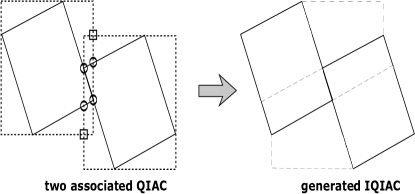
Figure 2: On the left: two associated QIAC, dotted rectangles are the QIAC minimal rectangles, points marked with squares are minimal rectangles intersections, and points marked with circles are intersections of minimal rectangles and internal boundaries. On the right: generated IQIAC.

The fact that QIAC and IQIAC could be thought as a set of SIAC, allows using a unified methodology for the treatment of SIAC. This is not the case for original SIAC or those generated from IAC.

3 Methodology proposed for the generation of the structured quadrilateral mesh

The proposed general process for generating the desired mesh, follows these steps:

1. Generating an initial cartesian grid

2. Processing the SIAC generated by the QIAC

3. Processing the SIAC generated by the IQIAC

4. Processing the IAC

5. Either processing the original SIAC or applying a global smoothing in case there are no original SIAC

Each of these steps is detailed below.

Initial cartesian grid.

The process starts with the generation of a standard cartesian grid with constant spacing in each direction. For each direction the spacing is a fraction of the minimal distance between the intersection points of the SIAC with the external boundaries, as shown, for example, in Fig.3. We denote by $m$ and $n$ the numbers of partition points in each direction. Thus, the initial cartesian grid has $mn$ nodes.

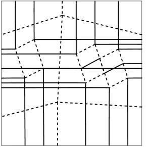
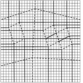
Figure 3: On the left: internal boundaries identified with dotted lines, three SIAC, one QIAC and one IQIAC. All vertical and horizontal lines of either a QIAC or an IQIAC are extended to the external boundaries to form SIAC. On the right: Example of the initial cartesian grid based on the internal boundaries.

Processing the SIAC and IAC.

As it was explained in the last section, the QIAC and IQIAC are decomposed into a set of SIAC, while the IAC are extended to the external boundaries to form SIAC. Consequently, the processing of all these internal boundaries is reduced to the treatment of a set of SIAC. The aim of the SIAC treatment is to adjust the nodes of the initial cartesian grid to this set of SIAC.

This procedure consists of three essential steps:

• association of lines,

• redistribution of nodes on associated lines, and

• labelling of fixed nodes

Association of lines.

Given, for example, a horizontal SIAC, the idea is to associate a line in the cartesian grid that best adjust to that SIAC. To achive this, calculate the mean of the vertices ordinates of the SIAC and then choose a line of the cartesian grid whose ordinate is the closest to that mean. In the case of a vertical SIAC, proceeds in similar way. See the top-left image in Fig.4.

Figure 4: Gray lines conform the initial catersian grid, dotted lines are internal boundaries (SIAC). Top-left: thick lines of the mesh represent associated lines to each SIAC. Top-right: mapping the mesh nodes of the upper horizontal associated line on the SIAC. Bottom-left: overlap mesh generated from the three SIAC. Bottom-right: overlap mesh generated from the three SIAC and the external boundaries.

Redistribution of nodes on the associated line.

First, the end vertices of the SIAC are associated to the end points of the associated line. Second, each internal vertex of the SIAC will be assigned to the closest internal node of the associated line. Therefore, a partition is created on each associated line, based on the vertices of the SIAC. Finally, for each SIAC and associated line, one proceeds as follows: the nodes for each pair of consecutive internal vertices on the associated line, are distributed in a proportional way over the corresponding segment of the SIAC, see top-right and bottom-left images in Fig.4.

It is important to point out that a vertex corresponding to the intersection of two SIAC, is always associated to the intersection of the two associated lines.

A similar redistribution procedure applies to the external boundary nodes.

Therefore an overlap mesh, coming from the deformation of the initial cartesian grid, is obtained (see bottom-right image in Fig.4).

Labelling of fixed nodes.

Some of the nodes of the overlap grid must be labeled, because they will be fixed during the smoothing process. The fixed nodes are either the ones coming from the original internal boundaries (IAC, QIAC, IQIAC and original SIAC) or those belonging to the external boundary. This labelling information will play an important role in the resolution of the non linear system arising from the discretization of the elliptic partial differential equation in the smoothing process.

Smoothing process.

This process seeks to relocate in a smooth manner the nodes belonging to the overlapping mesh in order to get the quadrilateral mesh, structured, conformal and tailored to the internal boundaries of $\Omega$.

The transformation of the physical plane $(x,y)$ (overlapping mesh) to the transformed plane $(\xi,\eta)$ (smooth mesh) is given by the vector function $f(x,y)=(\xi,\eta)$, with $\xi=\xi(x,y)$, $\eta=\eta(x,y)$. Similarly, the inverse transformation is given by the functions $x=x(\xi,\eta)$, $y=y(\xi,\eta)$. The Jacobian matrix of the inverse transformation is given by

$$\frac{\partial(x,y)}{\partial(\xi,\eta)}=\begin{pmatrix}x_{\xi}&x_{\eta}\\ y_{\xi}&y_{\eta}\end{pmatrix},$$

and $J=\det\frac{\partial(x,y)}{\partial(\xi,\eta)}=x_{\xi}y_{\eta}-x_{\eta}y_{\xi}$, where it is imposed that $x_{\xi}y_{\eta}-x_{\eta}y_{\xi}\neq 0.$

The smooth mesh satisfies, see [29, 23, 24, 25], the standard system of elliptic equations

$$\begin{array}[]{l}\Delta\xi=\xi_{xx}+\xi_{yy}=0,\\ \Delta\eta=\eta_{xx}+\eta_{yy}=0,\end{array}$$ (1)

with Dirichlet type boundary conditions, corresponding to the positions of fixed nodes on the internal and external boundaries.

The tangent vectors at a point $P$ are defined by

$$e_{1}=(\frac{\partial x}{\partial\xi},\frac{\partial y}{\partial\xi})^{t}\ \ {\rm and}\ \ e_{2}=(\frac{\partial x}{\partial\eta},\frac{\partial y}{\partial\eta})^{t}\ .$$

These base vectors are called covariant base vectors.

A second set of vectors, $e^{1}$ and $e^{2}$, is defined by $e^{i}\cdot e_{j}=\delta_{j}^{i}$, $i,j=1,2$, with $\delta$ the Kronecker delta. The $e^{i}$ are called contravariant base vectors and are orthogonal to the respective covariant vector for $i\neq j$.

A vector $v$ can either be represented in the covariant or contravariant base vectors as

$$v=\sum_{i}v^{i}e_{i}=\sum_{j}v_{j}e^{j}\ ,$$

where $v^{i}$ and $v_{j}$ are their components respectively.

Let’s define the matrix ($g_{ij}$) as $g_{ij}=e_{i}\cdot e_{j}$ for $i,j=1,2$, then $g=\det(g_{ij})=g_{11}g_{22}-g_{12}^{2}$. It follows,

$$\begin{array}[]{l}g_{11}=(x_{\xi})^{2}+(y_{\xi})^{2},\ \ g_{12}=g_{21}=x_{\xi}x_{\eta}+y_{\xi}y_{\eta},\ \ g_{22}=(x_{\eta})^{2}+(y_{\eta})^{2}\ ,\\ {\rm and}\ \ \ g=(x_{\xi}y_{\eta}-x_{\eta}y_{\xi})^{2}=J^{2}\ .\end{array}$$ (2)

The components of the inverse matrix ($g^{ik}$) of $(g_{ik})$ are found from

$$\sum_{i=1}^{2}g_{ij}g^{ik}=\delta_{j}^{k}\ .$$

Therefore, after some calculations,

$$g^{11}=g^{-1}g_{22},\ \ \ g^{12}=g^{21}=-g^{-1}g_{21},\ \ \ g^{22}=g^{-1}g_{11}\ .$$ (3)

Some of the lemmas and theorems 1 and 2 included in this subsection are for the sake of completeness (see [11]).

Lemma 2.

The Jacobian matrix of the transformation $f$ is

$$\frac{\partial(\xi,\eta)}{\partial(x,y)}=\begin{pmatrix}\xi_{x}&\xi_{y}\\ \eta_{x}&\eta_{y}\end{pmatrix}=J^{-1}\begin{pmatrix}y_{\eta}&-x_{\eta}\\ -y_{\xi}&x_{\xi}\end{pmatrix},$$ (4)

with $J=x_{\xi}y_{\eta}-y_{\xi}x_{\eta}$.

Proof.

let $a$, $b$, $c$ and $d$ be the components of the inverse matrix of $\frac{\partial(x,y)}{\partial(\xi,\eta)}$, i.e.

$$\begin{pmatrix}a&b\\ c&d\end{pmatrix}\begin{pmatrix}x_{\xi}&x_{\eta}\\ y_{\xi}&y_{\eta}\end{pmatrix}=\begin{pmatrix}1&0\\ 0&1\end{pmatrix}.$$

After some calculations it follows

$$a=J^{-1}y_{\eta},\ \ b=-J^{-1}x_{\eta},\ \ c=-J^{-1}y_{\xi},\ \ d=J^{-1}x_{\xi}.$$

From the definition of $e^{i}$, i.e. $e^{i}\cdot e_{j}=\delta_{j}^{i}$, $i,j=1,2$, it follows

$$e^{1}=(a,b)^{t}=J^{-1}\begin{pmatrix}y_{\eta}\\ -x_{\eta}\end{pmatrix}\ \ {\rm and}\ \ e^{2}=(c,d)^{t}=\begin{pmatrix}-y_{\xi}\\ x_{\xi}\end{pmatrix},$$

and finally,

$$\frac{\partial(\xi,\eta)}{\partial(x,y)}=\begin{pmatrix}\xi_{x}&\xi_{y}\\ \eta_{x}&\eta_{y}\end{pmatrix}=J^{-1}\begin{pmatrix}y_{\eta}&-x_{\eta}\\ -y_{\xi}&x_{\xi}\end{pmatrix}.$$

∎

Theorem 1.

The non-linear inverted differential equations corresponding to the Laplacian equations (1), with Dirichlet type boundary conditions, are

$$\begin{array}[]{l}Lx\equiv\alpha x_{\xi\xi}-2\beta x_{\xi\eta}+\gamma x_{\eta\eta}=0,\\ Ly\equiv\alpha y_{\xi\xi}-2\beta y_{\xi\eta}+\gamma y_{\eta\eta}=0,\end{array}$$ (5)

where $\alpha=x_{\eta}^{2}+y_{\eta}^{2}$, $\beta=x_{\xi}x_{\eta}+y_{\xi}y_{\eta}$ and $\gamma=x_{\xi}^{2}+y_{\xi}^{2}$, and with transformed boundary conditions.

Proof.

the equations (1) are analytically inverted and the calculations are carried out in the physical plane (overlapping mesh).

Given a twice differentiable and continuous scalar function $h$ from $\Omega=[a,b]\times[c,d]\subset\mathbb{R}^{2}$ into $\mathbb{R}$, such that $\Delta h=0$, then

$$\nabla h=e^{1}\frac{\partial h}{\partial\xi}+e^{2}\frac{\partial h}{\partial\eta}=e_{1}v^{1}+e_{2}v^{2}\ ,$$

where

$$v^{1}=(e^{1}\frac{\partial h}{\partial\xi}+e^{2}\frac{\partial h}{\partial\eta})\cdot e^{1}=e^{1}\cdot e^{1}\frac{\partial h}{\partial\xi}+e^{2}\cdot e^{1}\frac{\partial h}{\partial\eta}\ ,$$

$$v^{2}=(e^{1}\frac{\partial h}{\partial\xi}+e^{2}\frac{\partial h}{\partial\eta})\cdot e^{2}=e^{1}\cdot e^{2}\frac{\partial h}{\partial\xi}+e^{2}\cdot e^{2}\frac{\partial h}{\partial\eta}\ .$$

Calculating the Laplacian of $h$

$$\Delta h=\nabla\cdot(\nabla h)=e^{1}\cdot\frac{\partial}{\partial\xi}(e_{1}v^{1}+e_{2}v^{2})+e^{2}\cdot\frac{\partial}{\partial\eta}(e_{1}v^{1}+e_{2}v^{2})=$$

$$\frac{\partial}{\partial\xi}v_{1}e^{1}\cdot e_{1}+\frac{\partial}{\partial\xi}v_{2}e^{1}\cdot e_{2}+\frac{\partial}{\partial\eta}v_{1}e^{2}\cdot e_{1}+\frac{\partial}{\partial\eta}v_{2}e^{2}\cdot e_{2}=$$

$$e^{1}\cdot e^{1}\frac{\partial^{2}h}{\partial\xi^{2}}+2e^{2}\cdot e^{1}\frac{\partial^{2}h}{\partial\xi\partial\eta}+e^{2}\cdot e^{2}\frac{\partial^{2}h}{\partial\eta^{2}}\ .$$

The terms $e^{1}\cdot e^{1}$, $e^{2}\cdot e^{2}$ and $e^{2}\cdot e^{1}$ are

$$e^{1}\cdot e^{1}=(J^{-1})^{2}(x_{\eta}^{2}+y_{\eta}^{2}),\ \ e^{2}\cdot e^{2}=(J^{-1})^{2}(x_{\xi}^{2}+y_{\xi}^{2}),$$

$${\rm and}\ \ e^{2}\cdot e^{1}=-(J^{-1})^{2}(x_{\xi}x_{\eta}+y_{\xi}y_{\eta}).$$

Now, defining $\alpha=x_{\eta}^{2}+y_{\eta}^{2}$, $\beta=x_{\xi}x_{\eta}+y_{\xi}y_{\eta}$ and $\gamma=x_{\xi}^{2}+y_{\xi}^{2}$, and using that $\Delta h=0$, follows

$$\alpha\frac{\partial^{2}h}{\partial\xi^{2}}-2\beta\frac{\partial^{2}h}{\partial\xi\partial\eta}+\gamma\frac{\partial^{2}h}{\partial\eta^{2}}=0\ .$$

Finally, the non-linear inverted differential equations (5) follows directly, for the functions $\xi$ and $\eta$ of the transformation $f$ together with equations (1). ∎

In the proof of Theorem 1, formulas for $e^{1}\cdot e^{1}$, $e^{2}\cdot e^{2}$ and $e^{2}\cdot e^{1}$ were deduced. This results together with equations (3), implies that

$$e^{1}\cdot e^{1}=(J^{-1})^{2}(x_{\eta}^{2}+y_{\eta}^{2})=g^{-1}g_{22}=g^{11},$$

$$e^{2}\cdot e^{2}=(J^{-1})^{2}(x_{\xi}^{2}+y_{\xi}^{2})=g^{-1}g_{11}=g^{22},$$

$${\rm and}\ \ e^{2}\cdot e^{1}=-(J^{-1})^{2}(x_{\xi}x_{\eta}+y_{\xi}y_{\eta})=-g^{-1}g_{21}=g^{21}.$$

Then, $g^{ij}=e^{i}\cdot e^{j}$ for $i,j=1,2$, i.e. the components of the inverse matrix of the matrix $(g_{ij})$ can be calculated by inner products of the contravariant base vectors.

Lemma 3.

The equations (5) in Theorem 1 are elliptic.

Discretization.

The equations in (5) are coupled and nonlinear. The unknowns are the positions of the mesh nodes in the physical plane $x$ and $y$.

Definition 7.

Given a twice differentiable and continuous scalar function $x$ from $\Omega=[a,b]\times[c,d]\subset\mathbb{R}^{2}$ into $\mathbb{R}$, let’s define the first and second order finite difference operators of $x$ with respect to $\xi$ and $\eta$ as follows

$$\begin{array}[]{l}x_{\overline{\xi}}(\xi,\eta)\equiv\frac{x(\xi+\Delta\xi,\eta)-x(\xi-\Delta\xi,\eta)}{2\Delta\xi},\\ x_{\overline{\eta}}(\xi,\eta)\equiv\frac{x(\xi,\eta+\Delta\eta)-x(\xi,\eta-\Delta\eta)}{2\Delta\eta},\\ x_{\overline{\xi\xi}}(\xi,\eta)\equiv\frac{x(\xi+\Delta\xi,\eta)-2x(\xi,\eta)+x(\xi-\Delta\xi,\eta)}{(\Delta\xi)^{2}},\\ x_{\overline{\eta\eta}}(\xi,\eta)\equiv\frac{x(\xi,\eta+\Delta\eta)-2x(\xi,\eta)+x(\xi,\eta-\Delta\eta)}{(\Delta\eta)^{2}},\\ x_{\overline{\xi\eta}}(\xi,\eta)\equiv\frac{x(\xi+\Delta\xi,\eta+\Delta\eta)-x(\xi+\Delta\xi,\eta-\Delta\eta)+x(\xi-\Delta\xi,\eta-\Delta\eta)-x(\xi-\Delta\xi,\eta+\Delta\eta)}{4\;\Delta\xi\Delta\eta}.\end{array}$$ (6)

where $\Delta\xi$ and $\Delta\eta$ are the constant spacings in the $\xi$ and $\eta$ directions respectively.

Lemma 4.

Given a twice differentiable and continuous scalar function $x$ from $\Omega=[a,b]\times[c,d]\subset\mathbb{R}^{2}$ into $\mathbb{R}$, the approximation errors for the first and second derivatives of $x$, using the finite difference operators (6) given in definition 7, are order 2.

Remark 3.

Lemmas 3 and 4 are sufficiently known results, and their proofs are straightforward.

Lemma 5.

Given a twice differentiable and continuous scalar function $x$ from $\Omega=[a,b]\times[c,d]\subset\mathbb{R}^{2}$ into $\mathbb{R}$, the operator

$$Lx\equiv\alpha x_{\xi\xi}-2\beta x_{\xi\eta}+\gamma x_{\eta\eta}$$

can be approximated by

$$L_{h}x\equiv\alpha x_{\overline{\xi\xi}}-2\beta x_{\overline{\xi\eta}}+\gamma x_{\overline{\eta\eta}}$$

with an approximation error of order 2, where $x_{\overline{\xi\xi}}$, $x_{\overline{\xi\eta}}$ and $x_{\overline{\eta\eta}}$ are the finite differences (6) in definition 7.

Proof.

the proof follows from a straightforward calculation using the results in lemma 4

$$L_{h}x-Lx=\alpha(x_{\overline{\xi\xi}}-x_{\xi\xi})-2\beta(x_{\overline{\xi\eta}}-x_{\xi\eta})+\gamma(x_{\overline{\eta\eta}}-x_{\eta\eta})=O((\Delta\xi)^{2}+(\Delta\eta)^{2}).\qed$$

Theorem 2.

The discrete version of the system of equations (5), for any vertex $(i,j)$ of the mesh in the physical plane, can be written as follows

$$\begin{array}[]{l}2(x_{i+1,j}-2x_{i,j}+x_{i-1,j})\cdot((x_{i,j+1}-x_{i,j-1})^{2}+(y_{i,j+1}-y_{i,j-1})^{2})-\\ -(x_{i+1,j+1}-x_{i+1,j-1}+x_{i-1,j-1}-x_{i-1,j+1})\cdot\\ \cdot((x_{i+1,j}-x_{i-1,j})\cdot(x_{i,j+1}-x_{i,j-1})+\\ +(y_{i+1,j}-y_{i-1,j})\cdot(y_{i,j+1}-y_{i,j-1}))+\\ +2(x_{i,j+1}-2x_{i,j}+x_{i,j-1})\cdot\\ \cdot((x_{i+1,j}-x_{i-1,j})^{2}+(y_{i+1,j}-y_{i-1,j})^{2})=0,\end{array}$$ (7)

$$\begin{array}[]{l}2(y_{i+1,j}-2y_{i,j}+y_{i-1,j})\cdot((x_{i,j+1}-x_{i,j-1})^{2}+(y_{i,j+1}-y_{i,j-1})^{2})-\\ -(y_{i+1,j+1}-y_{i+1,j-1}+y_{i-1,j-1}-y_{i-1,j+1})\cdot\\ \cdot((x_{i+1,j}-x_{i-1,j})\cdot(x_{i,j+1}-x_{i,j-1})+\\ +(y_{i+1,j}-y_{i-1,j})\cdot(y_{i,j+1}-y_{i,j-1}))+\\ +2(y_{i,j+1}-2y_{i,j}+y_{i,j-1})\cdot((x_{i+1,j}-x_{i-1,j})^{2}+(y_{i+1,j}-y_{i-1,j})^{2})=0.\end{array}$$ (8)

Proof.

the finite differences (6) given in definition 7 are used to approximate the derivatives appearing in the set of elliptic equations (5) in the physical plane.

After some calculations, the discrete version (7-8) of the system of equations (5) is obtained. ∎

The nonlinear system (7-8) consists of $2mn$ equations, where $m$ and $n$ are the dimensions of the initial cartesian grid. In this nonlinear system, the coordinates of the vertices on the internal and external boundaries are fixed. If $p$ is the number of fixed vertices, then the final nonlinear system has $r=2(mn-p)$ equations and unknowns. These unknowns correspond to the coordinates of the overlapping mesh nodes which are not fixed (i.e. those which are not vertices).

4 Algorithms

The general process for generating the mesh honoring the internal boundaries, given in section 3, can be translated into the following algorithm. This algorithm was implemented in fortran 90.

1. Decompose the QIAC and IQIAC into a set of SIAC

2. Extend the IAC to the external boundaries to form SIAC

3. Generate the initial uniform cartesian grid

4. For each SIAC (including the original SIAC)

   1. Associate a line from the initial grid

   2. Redistribute the nodes on the associated line into the SIAC

5. Redistribute nodes on the external boundaries

6. Smooth the overlapping mesh

In item 4 it is important to point out that the treatment is slightly different for SIAC coming from QIAC or IQIAC. In this case, these QIAC or IQIAC are first enclosed in their minimal rectangles such that the processes of line association and redistribution of nodes happen locally. The overlapping local grid is then connected logically to the initial cartesian grid.

The smooth mesh is obtained by solving the set of elliptic equations (5) presented in section 3. As mentioned before, this set of elliptic equations is approximated by finite differences, conducing to the nonlinear system (7-8).

This system of nonlinear equations $F(v)=0$, with $F:\mathbf{R}^{r}\rightarrow\mathbf{R}^{r}$ and the vector $v$ representing the final coordinates of each node of the grid, is solved numerically by SANE (Spectral Approach for Nonlinear Equations) method (see [13]). The methodology is based on minimization techniques without restrictions, where the objective function involved is $g(v)=F(v)^{t}F(v)$. The key issue in this methodology is the combination between the search direction ($d_{k}=\pm F(x_{k})$) and the fact that the nonmonotone line search involves a quadratic interpolation. The Jacobian matrix of $F$ is, in general, non symmetric and large.

The SANE method, implemented in fortran 90, is presented in SANE Algorithm. It is important to remark that this algorithm only involves one smooth process, compared to previous works (see [9], [5] and [26]).

SANE Algorithm (see [13]).

Let	$\alpha_{0}\in\mathbf{R}$, $M\geq 0$, $\gamma>0$ and $0<\sigma_{1}<\sigma_{2}<1$, $0<\epsilon<1$
	and $\delta\in[\epsilon,\frac{1}{\epsilon}]$.
Let	$v_{0}\in\mathbf{R}^{r}$ be the initial guess and set $k=0$.
Step 1:	If $\left\|F_{k}\right\|=0$, stop the process.
Step 2:	If $\frac{|F_{k}^{t}\>J_{k}\>F_{k}|}{F_{k}^{t}\>F_{k}}<\epsilon$, stop the process.
Step 3:	If $\alpha_{k}\leq\epsilon$ or $\alpha_{k}\geq\frac{1}{\epsilon},$ then set $\alpha_{k}=\delta$.
Step 4:	Set $sgn_{k}=sgn(F_{k}^{t}\>J_{k}\>F_{k})$ and $d_{k}=-sgn_{k}\>F_{k}$.
Step 5:	Set $\lambda=\frac{1}{\alpha_{k}}$.
Step 6:	If $f(v_{k}+\lambda d_{k})\leq\max_{0\leq j\leq\min\{k,M\}}f(v_{k-j})+2\gamma\lambda\>F_{k}^{t}\>J_{k}\>d_{k}$,
	go to Step 8.
Step 7:	Choose $\sigma\in[\sigma_{1},\sigma_{2}]$, and set $\lambda=\sigma\lambda$. Now go to Step 6.
Step 8:	Set $\lambda_{k}=\lambda$, $v_{k+1}=v_{k}+\lambda_{k}\>d_{k}$, $w_{k}=F_{k+1}-F_{k}$.
Step 9:	Set $\alpha_{k+1}=sgn_{k}\left(\frac{d_{k}^{t}\>w_{k}}{\lambda_{k}\>d_{k}^{t}\>d_{k}}\right)$, $k=k+1$ and go to Step 1.

5 Examples and numerical results

Examples 1 to 4 presented in this section correspond to rectangular oil reservoirs. The internal boundaries to be considered are SIAC, QIAC and IQIAC and combinations of these. Example 1 (see Fig.5) includes two horizontal and one vertical SIAC, example 2 (see Fig.6) consists of one QIAC, example 3 (see Fig.7) contains three QIAC, and example 4 (see Fig.8) includes three SIAC, one QIAC, and one IQIAC. Table 1 shows the results obtained with SANE and the Newton-GMRES methodologies.

In Table 1, $||F||_{2}$ is the 2-norm of the function $F$, and $||M_{1}-M_{2}||_{\infty}$ corresponds to the infinite norm of the vector difference of the coordinates of the meshes obtained with both methodologies. $L$ represents the size of the domain (side length of the domain, in all cases the domain is a square). Additionally, N-GMRES means Newton’s method, nested with a GMRES type method.

Table 1. Comparison of SANE and Newton-GMRES methods.

Ex	Methods	$||F||_{2}$	$\frac{||M_{1}-M_{2}||_{\infty}}{L}$	Time
				Iterations
Ex 1	N-GMRES	$2.0425\times 10^{-1}$	$0.064585$	$0.9840$ sec
				8N / 8 GMRES
	SANE	$2.0430\times 10^{-1}$		$0.1100$ sec
				185
Ex 2	N-GMRES	$2.4367\times 10^{-2}$	$0.0082315$	$0.5310$ sec
				6N / 6 GMRES
	SANE	$2.4414\times 10^{-2}$		$0.0310$ sec
				107
Ex 3	N-GMRES	$6.2817\times 10^{-1}$	$0.055343$	$1.2970$ sec
				24N / 24 GMRES
	SANE	$5.3339\times 10^{-1}$		$0.0780$ sec
				93
Ex 4	N-GMRES	$2.6808\times 10^{-3}$	$1.16205$	$54.6710$ sec
				55N / 55 GMRES
	SANE	$2.8194\times 10^{-3}$		$0.4530$ sec
				152

Example 5 combines the use of QIAC with SIAC to model a channel of high permeability and the drainage areas of two producer wells in the vicinity of the channel (see Fig.9).

Example 6 represents a circumference shaped obstacle within a reservoir (see Fig.10) where the permeability could be low compared to the other areas of $\Omega$.

In both cases it is observed how good the mesh adapts to the internal boundary.

Buitrago et al. used this type of meshes to have a good representation of the internal structures of the reservoir and to solve the convection diffusion equation in two dimensions based on finite volume methods (see [6]).

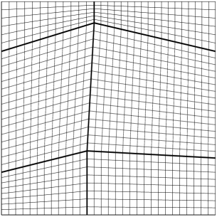
Figure 5: Example 1 with three SIAC, two horizontal and one vertical. On the right: the smooth mesh is supported on the internal boundaries.

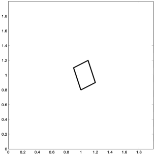
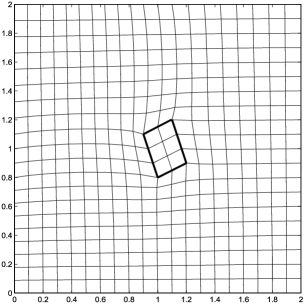
Figure 6: Example 2 with one QIAC. On the right: the smooth mesh is supported on the internal boundaries.

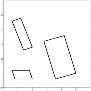
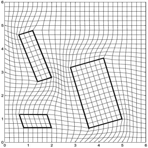
Figure 7: Example 3 with three QIAC. On the right: the smooth mesh is supported on the internal boundaries.

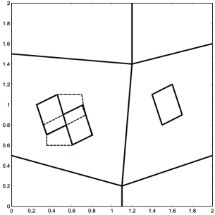
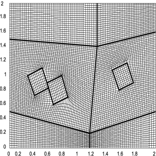
Figure 8: Example 4 with three SIAC, one QIAC, and one IQIAC. On the right: the smooth mesh is supported on the internal boundaries.

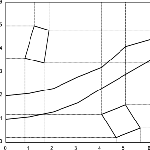
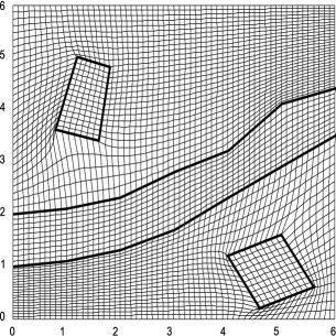
Figure 9: Example 5 with one channel and two QIAC. On the right: the smooth mesh is supported on the internal boundaries. This example models a channel of high permeability in a reservoir and the drainage areas of two producer wells in the vicinity of the channel.

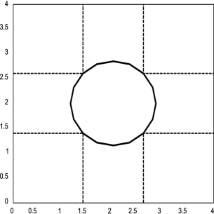
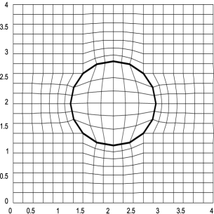
Figure 10: Example 6 with one circumference. On the right: the smooth mesh is supported on the internal boundaries. This example models a very low permeability obstacle within a reservoir.

6 Conclusions

1. The physical domain was discretized using non orthogonal structured (valence 4) grid consisting only of quadrilaterals honoring the internal structures of a reservoir.

2. The methodology does not need for previous step where triangles are generated.

3. The SANE algorithm is a robust option for solving the nonlinear system associated to the methodology for generation of 2D quadrilateral meshes adapted to internal boundaries. This does not involve nesting of iterative methods to solve the nonlinear system.

4. The mesh generation methodology involves a single smoothing process compared to previous works.

5. The methodology was implemented in fortran 90, taking advantage of the potential of the language to create structures adapted to the raised geometric problem.

6. Additionally, we suggest to explore the possibility of implementing a code that exploits the implicit parallelism in the methodology proposed in this paper. Particularly, the distribution of work that arises naturally, is to process each internal boundary on each processor of a cluster (parallel architecture computer).

References

References

- Amsden and Hirt [1973] A.A. Amsden and W. Hirt. A simple scheme for generating general curvilinear grids. Journal of Computational Physics, 11, 1973. doi: 10.1016/0021-9991(73)90078-8.
- Berndt et al. [2008] M. Berndt, J.D. Moulton, and G. Hansen. Efficient nonlinear solvers for Laplace-Beltrami smoothing of three-dimensional unstructured grids. Comput Math Appl, 55(12):2791–2806, 2008. http://math.lanl.gov/ berndt/Papers/setup-paper.pdf, doi: 10.1016/j.camwa.2007.10.029.