Temperature Structure in the Perseus Cluster Core Observed with Hitomi

Abstract

The present paper investigates the temperature structure of the X-ray emitting plasma in the core of the Perseus cluster using the 1.8–20.0 keV data obtained with the Soft X-ray Spectrometer (SXS) onboard the Hitomi Observatory. A series of four observations were carried out, with a total effective exposure time of 338 ks and covering a central region $\sim 7\arcmin$ in diameter. The SXS was operated with an energy resolution of $\sim$5 eV (full width at half maximum) at 5.9 keV. Not only fine structures of K-shell lines in He-like ions but also transitions from higher principal quantum numbers are clearly resolved from Si through Fe. This enables us to perform temperature diagnostics using the line ratios of Si, S, Ar, Ca, and Fe, and to provide the first direct measurement of the excitation temperature and ionization temperature in the Perseus cluster. The observed spectrum is roughly reproduced by a single temperature thermal plasma model in collisional ionization equilibrium, but detailed line ratio diagnostics reveal slight deviations from this approximation. In particular, the data exhibit an apparent trend of increasing ionization temperature with increasing atomic mass, as well as small differences between the ionization and excitation temperatures for Fe, the only element for which both temperatures can be measured. The best-fit two-temperature models suggest a combination of 3 and 5 keV gas, which is consistent with the idea that the observed small deviations from a single temperature approximation are due to the effects of projection of the known radial temperature gradient in the cluster core along the line of sight. Comparison with the Chandra/ACIS and the XMM-Newton/RGS results on the other hand suggests that additional lower-temperature components are present in the ICM but not detectable by Hitomi SXS given its 1.8–20 keV energy band.

1 Introduction

The X-ray emitting hot intracluster medium (ICM) dominates the baryonic mass in galaxy clusters, and its thermodynamical properties are crucial for studying the evolution of large-scale structure in the Universe. Discontinuities in the ICM temperature and density profiles reveal ongoing cluster mergers (Markevitch et al., 2000; Vikhlinin et al., 2001; Markevitch & Vikhlinin, 2007; Akamatsu & Kawahara, 2013), while the pressure profiles in the cluster outskirts are also key to understanding their growth (Arnaud et al., 2010; Simionescu et al., 2011; Planck Collaboration et al., 2013; Simionescu et al., 2017). The thermodynamical properties of the dense ICM at the centers of so-called “cool-core” clusters are even more complex; despite the fact that radiative cooling in these regions should be very efficient, stars are being formed at a rate smaller than that expected from the amount of hot ICM (e.g., Peterson et al. (2003)). The heating mechanism responsible for compensating the radiative cooling is under debate, and various ideas have been proposed, such as feedback from the active galactic nuclei (AGN) in the brightest cluster galaxies (e.g., McNamara & Nulsen (2007)), energy transfer from moving member galaxies (e.g, Makishima et al. (2001); Gu et al. (2013)), and cosmic-ray streaming with Alfvén waves (e.g., Fujita et al. (2013)). While less effective than expected, some radiative cooling likely does occur, and the presence of multi-phase ICM in cool-core clusters is also reported (Fukazawa et al., 1994; Sanders & Fabian, 2007; Takahashi et al., 2009; Gu et al., 2012; Sanders et al., 2016; Pinto et al., 2016).

To date, temperature measurements of the ICM have been mainly performed by fitting broad-band spectra (typically 0.5–10.0 keV band) obtained from X-ray CCDs. Because of the moderate energy resolution of this type of spectrometers, temperatures are mainly determined by shapes of the continuum and the Fe L-shell lines complex. However, the continuum shape is subject to uncertainties due to background modeling and/or effective area calibration (e.g., de Plaa et al. (2007); Leccardi & Molendi (2008); Nevalainen et al. (2010); Schellenberger et al. (2015)).

An independent estimate of the gas temperature can be obtained from the flux ratios of various emission lines, the so-called line ratio diagnostic; a ratio between different transitions in the same ion such as Ly$\alpha$-to-Ly$\beta$ indicates the excitation temperature, and a ratio of lines from different ionization stages such as He$\alpha$-to-Ly$\alpha$ represents the ion fraction (also referred to as the ionization temperature). These temperatures should match the temperature from the continuum shape when the observed plasma is truly single temperature in collisional ionization equilibrium (CIE). If there is a disagreement between those temperatures, deviation from a single CIE plasma is suggested: multi-temperature and/or non-equilibrium ionization (NEI). For instance, Matsushita et al. (2002) utilized the Si and S K-shell lines to measure the temperature profile in M 87. Ratios of K-shell lines from Fe were used for the Ophiuchus Cluster (Fujita et al., 2008), the Coma Cluster (Sato et al., 2011) and A754 (Inoue et al., 2016). In practice, this method has been applied to a relatively small number of lines because of line blending and because only the fluxes of the strongest lines are free from uncertainties in the exact continuum calibration and background subtraction.

The XMM-Newton Reflection Grating Spectrometers (RGS) offer higher spectral resolution and enable us to perform diagnostics with O K-shell and Fe L-shell lines, which are sensitive to the temperature range of $kT<1$ keV (e.g., Pinto et al. (2016)). However, the energy band of the RGS is limited to energies below 2 keV, and the energy resolution is degraded for diffuse sources due to the dispersive and slit-less nature of these spectrometers. Therefore, observations with a non-dispersive high-resolution spectrometer covering a broad energy band are desired for a precise characterization of the multi-temperature structure in the ICM.

The Hitomi satellite launched on February 2016 performed the first cluster observation of this kind, using its Soft X-ray Spectrometer (SXS). This non-dispersive microcalorimeter achieved spectral resolution of $\sim$5 eV in orbit (Porter et al. 2017), and observed the core of the Perseus cluster as its first light target. In the observed region, fine ICM substructures such as bubbles, ripples, and weak shock fronts were previously revealed by deep Chandra imaging (Fabian et al., 2011, and references therein). These features are thought to be due to the activity of the AGN in the cD galaxy NGC 1275, which is pumping out relativistic electrons that disturb and heat the surrounding X-ray gas. The presence of multiple phases structure in the ICM spanning a range of temperatures between $kT=0.5-8$ keV is also reported (Sanders & Fabian, 2007; Pinto et al., 2016).

The first measurement of Doppler shifts and broadening of the Fe-K emission lines from the Hitomi first-light data, reported in Hitomi Collaboration (2016) (hereafter the First paper), revealed that the line-of-sight velocity dispersion of the ICM in the core regions is unexpectedly low and subsonic. Constraints on an unidentified feature at 3.5 keV suggested to originate from dark matter (e.g., Bulbul et al. (2014)) are described by Hitomi Collaboration (2017). Using the full set of the Perseus data and the latest calibration, we have performed X-ray spectroscopy over the full Hitomi SXS band and report a series of follow-up papers. In this paper, we concentrate on measurements of the temperature structure in the cluster core. The high spectral resolution of the SXS allowed us to estimate the gas temperature based on seventeen independent line ratios from various chemical elements (Si through Fe). Companion papers report results on the metal abundances (Hitomi Collaboration 2017a, henceforth the Z paper), velocity fields (Hitomi Collaboration 2017b, the V paper), properties of the AGN in NGC1275 (Hitomi Collaboration 2017c, the AGN paper), the atomic code comparison (Hitomi Collaboration 2017d, the Atomic paper), and the detection of resonance scattering (Hitomi Collaboration 2017e, the RS paper).

Throughout this paper, we assume a cluster redshift of 0.017284 (see Appendix 1 of the V paper) and a Hubble constant of 70 km s^-1 Mpc^-1. Therefore, 1$\arcmin$ corresponds to the physical scale of 21 kpc. We use the 68% ($1\sigma$) confidence level for errors, but upper and lower limits are shown at the 99.7% ($3\sigma$) confidence level. X-ray energies in spectra are denoted at the observed (hence redshifted) frame rather than the object’s rest-frame.

2 Observation and Data Reduction

2.1 Hitomi Observation

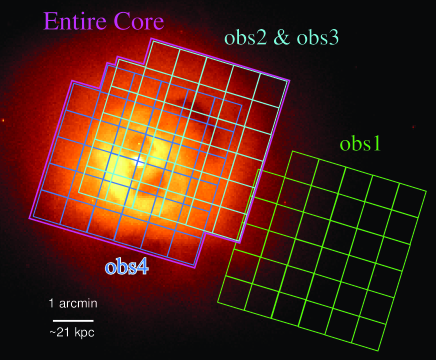
We observed the Perseus cluster four times with Hitomi/SXS during the commissioning phase in 2016 February and March (Table 2.1). The aim points of each observation are shown in Figure 1. The first light observation of Hitomi (obs1), is offset by $\sim 3\arcmin$ from the center of the Perseus cluster because the attitude control system was not commissioned at that time. In the next observation (obs2), the pointing direction was adjusted so that the Perseus core was in the SXS field-of-view (FoV). The same region was observed again after extension of the Hitomi Hard X-ray Detector’s optical bench (obs3). The obs3 is divided into the three sequential data sets (100040030, 100040040, and 100040050) solely for convenience in pipeline processing. In the final observation (obs4), the aim point was fine-tuned again to place the Perseus core at the center of the SXS FoV.

The SXS sensor is a $6\times 6$ pixel array (Kelley et al. 2017). Combined with the X-ray focusing mirror (Okajima et al., 2016), the SXS has a $3\arcmin\times 3\arcmin$ FoV with an angular resolution of $1.2\arcmin$ (half power diameter). One corner pixel is always illuminated by a dedicated ⁵⁵Fe source to track the gain variation with detector temperature, and is not used for astrophysical spectra. The SXS achieved the unprecedented energy resolution of $5$ eV (full width at half maximum) at 5.9 keV in orbit (Porter et al. 2017). The required energy bandpass of the SXS was 0.3–12 keV. During the early-mission observations discussed here, a gate valve remained closed to minimize the risk of contamination from outgassing in the spacecraft. The valve includes a Be window that absorbs most X-rays below   2 keV (Eckart et al., 2017).

The other instruments on Hitomi (Takahashi et al. 2017) were not yet operational during most or all of the Perseus observations described here.

List of observations. Name Observation ID $\alpha_{2000.0}$ $\delta_{2000.0}$ Observation Date Effective Exposure (deg) (deg) (ks) Hitomi/SXS obs1 100040010 49.878 41.484 2016-02-24 – 2016-02-25 49 obs2 100040020 49.935 41.519 2016-02-25 – 2016-02-27 97 obs3 100040030, 100040040, 100040050 49.936 41.520 2016-03-04 – 2016-03-06 146 obs4 100040060 49.955 41.512 2016-03-06 – 2016-03-07 46 Chandra/ACIS-I $\cdots$ 11714 49.928 41.569 2009-12-07 – 2009-12-08 92 XMM-Newton/RGS $\cdots$ 0085110101, 0085110201 49.951 41.512 2001-01-30 – 2001-01-31 72 $\cdots$ 0305780101 49.950 41.513 2006-01-29 – 2006-01-31 125

(a)

(b)

Figure 1: (left) SXS FoVs of the Hitomi observations overlaid on the Chandra X-ray color image in the 1.8–9.0 keV band. The green, cyan, and blue polygons indicate obs1, obs2 and obs3, and obs4, respectively. The 35 square boxes in each FoV correspond to the SXS pixels. The Entire core region covering the whole obs2/obs3 and obs4 is also shown in magenta. (right) Analysis regions used in Section 3.3 overlaid on the same Chandra image. The H$\alpha$ emission obtained with the WIYN 3.5 m telescope (Conselice et al., 2001) is also shown in the black contours. The cyan, blue, and green polygons corresponds to the Nebula, Rim, and Outer regions, respectively. For Nebula and Rim regions, we used slightly different sky regions between obs2/obs3 and obs4; the regions with solid line are for obs2/obs3 and those with dashed line are for obs4 (see text for details).

2.2 Hitomi Data Reduction

Figure 2: SXS 1–32 keV spectrum in the Entire core region (red). The corresponding non X-ray background estimated by sxsnxbgen is also plotted in black.

We used the cleaned event list provided by the pipeline processing version 03.01.006.007, and applied the additional screening described below using the HEAsoft version 6.21, Hitomi software version 6, and Hitomi calibration database version 7 (Angelini et al. 2017).

The SXS recorded signals up to 32 keV, but the standard pipeline processing reduces the energy coverage to the 0–16 keV band in order to achieve a sufficiently fine energy bin with the realistic number of channels in the nominal energy band (32768 bins with 0.5 eV bin^-1). However, the SXS was sensitive to bright sources above 16 keV because of its very low non-X-ray background (Kilbourne et al., 2017). We thus used a coarser bin size of 1.0 eV bin^-1 to extend the energy coverage up to 32 keV instead. This was technically achieved by the sxsextend ftools task. We confirmed that choosing the coarser bin size has no impact on our analysis due to intrinsic thermal and velocity broadening of lines.

We then applied event screening based on a pulse rise time versus energy relationship tuned for the wider energy coverage. We also selected only high primary grade events, for which arrival time between signal pulses was sufficiently large and hence the best spectroscopic performance was achieved. The branching ratio to other grades was less than 2% for the Perseus observations, so this grade selection hardly reduced the effective exposure.

Since the in-flight calibration of the SXS is limited, there is uncertainty of the gain scale especially at energies far from 5.9 keV. In addition, the SXS was not in thermal equilibrium during obs1 and obs2, and thus a $\sim$2 eV gain shift was seen even at 5.9 keV (Fujimoto et al. 2017). In order to correct for the gain scale, we applied the pixel-by-pixel redshift correction and the gain correction using a parabolic function as described in Appendix A.

We defined the four spectral analysis regions shown as the colour polygons in Figure 1. The Entire core region is the sum of the FoVs of obs2, obs3, and obs4 to maximize the photon statistics. In order to investigate the spatial variation of the temperature, we divided the Entire core region into two sub-regions: the Nebula region associated with the H$\alpha$ nebula (Conselice et al., 2001), and the Rim region located just outside the core, including the bubble seen north-west of the cluster center. The aim point of obs4 is different from that of obs2/3 by $\sim 60\arcsec$; thus, for the Nebula and Rim regions, spectra of obs2/3 and obs4 were extracted using slightly different spatial regions, and later co-added. Lastly the fourth region, which we refer to as the Outer region, is the entire FoV of obs1.

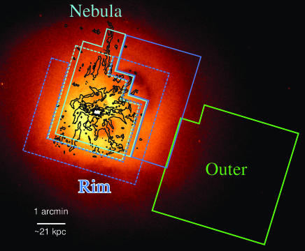
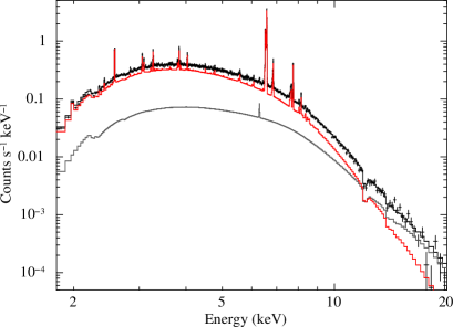
Non X-ray backgrounds (NXB) corresponding to each region were produced from the Earth eclipsed durations using sxsnxbgen. The redistribution matrix file (RMF) and the auxiliary response file (ARF) for spectral analysis were generated by sxsmkrmf and aharfgen, respectively. As an input to the ARF generator, we used the 1.8–9.0 keV Chandra image in which the AGN region ($r=10\arcsec$) is replaced with average adjacent brightness. The spectrum of the Entire core region with the corresponding non X-ray background is shown in Figure 2. The cluster is clearly detected above the NXB up to 20 keV. The attenuation below $\sim 2$ keV due to the closed gate valve can also be seen. For our analysis, we thus focus on the energy band spanning 1.8–20.0 keV.

2.3 Chandra and XMM-Newton Archive Data

For comparison with the Hitomi results, we also analyzed archival data from Chandra and XMM-Newton. Details of the observations are summarized in Table 2.1.

We reprocessed the Chandra data with CIAO version 4.9 software package and calibration database version 4.7.4. Spectra were extracted from the Nebula and Rim regions shown in Figure 1. A $9\arcsec$ radius circle around the central AGN region was excluded from the analysis taking advantage of Chandra’s spatial resolution. The spectra were binned so that each bin includes at least 100 counts. Background spectra were generated from the blank-sky observations provided in the calibration database, and were scaled so that their count rates in the 10–12 keV band match the source spectra.

We followed the data analysis methods of the CHEERS collaboration (de Plaa et al., 2017) for the reduction of the XMM-Newton/RGS data with the SAS version 14.0.0 software package. We extracted RGS source spectra in a region centered on the peak of the source emission, with a width of $0.8\arcmin$ in the cross-dispersion direction. While this is much smaller than the region probed by the SXS, a narrower extraction region in the cross-dispersion direction provides spectra that are least broadened by the spatial extent of the source, and thus have the best resolution. To further correct for this broadening, we used the lpro model component in SPEX to convolve the spectral models with the surface brightness profile extracted from the XMM-Newton MOS1 detector. We used background spectra generated by the SAS rgsbkgmodel task. The template background files were scaled using the count rates measured in the off-axis region of CCD9, in which the soft protons dominate the light curve.

3 Analysis and Results

The procedures described below were used for the spectral analysis presented in this section, unless stated otherwise. Spectral fits were performed using the Xspec 12.9.1h package (Arnaud, 1996) employing the modified C-statistic (Cash, 1979) in which a Poisson background spectrum is taken into account (also referred to as the W-statistic). We used the atomic databases of the AtomDB version 3.0.9 (Foster et al., 2012) and SPEXACT version 3.03.00 (Kaastra et al., 1996) for calculations of plasma models. We take differences between the model predictions as an estimate of model uncertainties. A python program was used to generate APEC format table models from SPEX , allowing us to perform a direct comparison of the results using a consistent treatment of all other assumptions and fit procedures.

Photoelectric absorption by cold matter in our Galaxy was modeled using the TBabs code version 2.3 (Wilms et al., 2000), in which fine-structures of absorption edges and cross-sections of dust grains and molecules are included. Its hydrogen column density was fixed at $1.38\times 10^{21}$ cm^-2 in accordance with the all-sky H I survey (Kalberla et al., 2005). We also considered the contaminating emission from the AGN in NGC 1275. Its spectrum was modeled using a power-law continuum and a neutral Fe K$\alpha$ line with parameters fixed at the values described in the AGN paper. Its flux was estimated by ray-tracing simulations (aharfgen).

3.1 Line Ratio Diagnostics

(a)

(b)

(c)

Figure 3: SXS spectra extracted from the Entire core region in the 1.8–3.0 keV (top left), 3.0–4.8 keV (top right), and 6.4–8.5 keV (bottom) bands. The fitted phenomenological models are shown by the red solid curves. The Gaussians included in the model are also plotted by the black dotted lines.

List of lines considered for the Gaussian fit. Line name $E_{0}$ Constraints (eV) Tied to Center Width Flux Si XIII w 1865.0 - - - - Si XIV Ly$\alpha_{1}$ 2006.1 - - - - Si XIV Ly$\alpha_{2}$ 2004.3 Si XIV Ly$\alpha_{1}$ $-1.8$ eV $\times 1.0$ $\times 0.5$ Si XIV Ly$\beta_{1}$ 2376.6 - - - - Si XIV Ly$\beta_{2}$ 2376.1 Si XIV Ly$\beta_{1}$ $-0.5$ eV $\times 1.0$ $\times 0.5$ S XV w 2460.6 - - - - S XVI Ly$\alpha_{1}$ 2622.7 - - - - S XVI Ly$\alpha_{2}$ 2619.7 S XVI Ly$\alpha_{1}$ $-3.0$ eV $\times 1.0$ $\times 0.5$ S XVI Ly$\beta_{1}$ 3106.7 - - - - S XVI Ly$\beta_{2}$ 3105.8 S XVI Ly$\beta_{1}$ $-0.9$ eV $\times 1.0$ $\times 0.5$ S XVI Ly$\gamma_{1}$ 3276.3 - - - - S XVI Ly$\gamma_{2}$ 3275.9 S XVI Ly$\gamma_{1}$ $-0.4$ eV $\times 1.0$ $\times 0.5$ Ar XVII w 3139.6 - - - - Ar XVIII Ly$\alpha_{1}$ 3323.0 - - - - Ar XVIII Ly$\alpha_{2}$ 3328.2 Ar XVIII Ly$\alpha_{1}$ $-4.8$ eV $\times 1.0$ $\times 0.5$ Ar XVIII Ly$\beta_{1}$ 3935.7 - - - - Ar XVIII Ly$\beta_{2}$ 3934.3 Ar XVIII Ly$\beta_{1}$ $-1.4$ eV $\times 1.0$ $\times 0.5$ Ca XIX w 3902.4 - - - - Ca XIX He$\beta_{1}$ 4583.5 - - - - Ca XX Ly$\alpha_{1}$ 4107.5 - - - - Ca XX Ly$\alpha_{2}$ 4100.1 Ca XX Ly$\alpha_{1}$ $-7.4$ eV $\times 1.0$ $\times 0.5$ Fe XXV z 6636.6 - - - - Fe XXV w 6700.4 - - - - Fe XXV He$\beta_{1}$ 7881.5 - - - - Fe XXV He$\beta_{2}$ 7872.0 Fe XXV He$\beta_{1}$ $-9.5$ eV $\times 1.0$ - Fe XXV He$\gamma_{1}$ 8295.5 - - - - Fe XXV He$\delta_{1}$ 8487.4 - - - - Fe XXV He$\epsilon_{1}$ 8588.5 - - - - Fe XXVI Ly$\alpha_{1}$ 6973.1 - - - - Fe XXVI Ly$\alpha_{2}$ 6951.9 Fe XXVI Ly$\alpha_{1}$ - $\times 1.0$ - Fe XXVI Ly$\beta_{1}$ 8252.6 - - - - Fe XXVI Ly$\beta_{2}$ 8248.4 Fe XXVI Ly$\beta_{1}$ $-6.2$ eV $\times 1.0$ - Ni XXVII w 7805.6 - - - - Constraints only on the Rim region Si XIII w 1865.0 Si XIV Ly$\alpha_{1}$ fixed at $E_{0}$ $\times 1.0$ - Ca XIX He$\beta_{1}$ 4583.5 Ca XX Ly$\alpha_{1}$ fixed at $E_{0}$ $\times 1.0$ - Constraints only on the Outer region Si XIII w 1865.0 Si XIV Ly$\alpha_{1}$ fixed at $E_{0}$ $\times 1.0$ - S XV w 2460.6 S XVI Ly$\alpha_{1}$ fixed at $E_{0}$ $\times 1.0$ - Ca XIX He$\beta_{1}$ 4583.5 Ca XX Ly$\alpha_{1}$ fixed at $E_{0}$ $\times 1.0$ - Fe XXV He$\gamma_{1}$ 8295.5 Fe XXV He$\beta_{1}$ fixed at $E_{0}$ $\times 1.0$ - Fe XXV He$\delta_{1}$ 8487.4 Fe XXV He$\beta_{1}$ fixed at $E_{0}$ $\times 1.0$ - Fe XXV He$\epsilon_{1}$ 8588.5 Fe XXV He$\beta_{1}$ fixed at $E_{0}$ $\times 1.0$ - Free parameters are denoted by the hyphen (-).

Fiducial energies of the emission lines at the rest frame in AtomDB 3.0.9

Ca XIX He$\beta_{2}$, Fe XXV He$\gamma_{2}$, Fe XXV He$\delta_{2}$, and Fe XXV He$\epsilon_{2}$ were omitted because their fluxes are too small to constrain from the SXS spetra.

Observed line fluxes derived from Gaussian fits. Line name Flux (10^-5 ph cm^-2 s^-1) Entire Core Nebula Rim Outer Si XIII w 6.40${}^{+4.71}_{-2.67}$ 5.87${}^{+3.60}_{-2.54}$ $<$5.45 $<$4.54 Si XIV Ly$\alpha_{1}$ 32.43${}^{+2.29}_{-2.23}$ 20.11${}^{+1.92}_{-1.83}$ 21.83${}^{+2.64}_{-2.52}$ 4.09${}^{+2.27}_{-1.72}$ Si XIV Ly$\beta_{1}$ 6.96${}^{+0.91}_{-0.87}$ 5.03${}^{+0.74}_{-0.70}$ 3.93${}^{+1.04}_{-0.98}$ 1.21${}^{+0.82}_{-0.58}$ S XV w 9.38${}^{+1.13}_{-1.11}$ 7.26${}^{+0.98}_{-0.99}$ 3.91${}^{+1.03}_{-0.94}$ $<$1.08 S XVI Ly$\alpha_{1}$ 22.71${}^{+0.73}_{-0.72}$ 15.81${}^{+0.64}_{-0.63}$ 12.46${}^{+0.77}_{-0.76}$ 2.70${}^{+0.67}_{-0.64}$ S XVI Ly$\beta_{1}$ 3.83${}^{+0.29}_{-0.29}$ 2.55${}^{+0.25}_{-0.24}$ 2.49${}^{+0.35}_{-0.33}$ 0.62${}^{+0.27}_{-0.22}$ S XVI Ly$\gamma_{1}$ 1.20${}^{+0.20}_{-0.19}$ 0.74${}^{+0.15}_{-0.17}$ 0.92${}^{+0.25}_{-0.24}$ 0.32${}^{+0.22}_{-0.17}$ Ar XVII w 3.72${}^{+0.37}_{-0.36}$ 2.82${}^{+0.31}_{-0.30}$ 1.87${}^{+0.51}_{-0.47}$ 1.20${}^{+0.41}_{-0.34}$ Ar XVIII Ly$\alpha_{1}$ 5.47${}^{+0.29}_{-0.29}$ 3.85${}^{+0.25}_{-0.25}$ 3.15${}^{+0.32}_{-0.30}$ 0.94${}^{+0.32}_{-0.30}$ Ar XVIII Ly$\beta_{1}$ 0.77${}^{+0.15}_{-0.15}$ 0.51${}^{+0.12}_{-0.12}$ 0.63${}^{+0.20}_{-0.18}$ 0.26${}^{+0.15}_{-0.11}$ Ca XIX w 5.20${}^{+0.27}_{-0.27}$ 3.66${}^{+0.23}_{-0.23}$ 2.94${}^{+0.30}_{-0.28}$ 0.93${}^{+0.29}_{-0.26}$ Ca XIX He$\beta_{1}$ 0.66${}^{+0.16}_{-0.10}$ 0.46${}^{+0.13}_{-0.10}$ 0.67${}^{+0.29}_{-0.35}$ 0.21${}^{+0.16}_{-0.12}$ Ca XX Ly$\alpha_{1}$ 2.80${}^{+0.18}_{-0.18}$ 1.85${}^{+0.16}_{-0.15}$ 1.81${}^{+0.20}_{-0.19}$ 0.77${}^{+0.20}_{-0.19}$ Fe XXV w 33.14${}^{+0.43}_{-0.34}$ 21.09${}^{+0.32}_{-0.31}$ 22.13${}^{+0.49}_{-0.35}$ 9.49${}^{+0.45}_{-0.44}$ Fe XXV z 13.26${}^{+0.27}_{-0.25}$ 8.72${}^{+0.21}_{-0.22}$ 8.41${}^{+0.28}_{-0.27}$ 3.03${}^{+0.28}_{-0.27}$ Fe XXV He$\beta_{1}$ 4.73${}^{+0.12}_{-0.24}$ 2.80${}^{+0.12}_{-0.15}$ 3.35${}^{+0.19}_{-0.18}$ 1.49${}^{+0.21}_{-0.20}$ Fe XXV He$\beta_{2}$ 1.04${}^{+0.10}_{-0.18}$ 0.73${}^{+0.14}_{-0.08}$ 0.55${}^{+0.13}_{-0.13}$ $<$0.17 Fe XXV He$\gamma_{1}$ 1.75${}^{+0.13}_{-0.13}$ 1.04${}^{+0.10}_{-0.10}$ 1.32${}^{+0.14}_{-0.13}$ 0.25${}^{+0.13}_{-0.12}$ Fe XXV He$\delta_{1}$ 0.88${}^{+0.12}_{-0.12}$ 0.55${}^{+0.10}_{-0.10}$ 0.63${}^{+0.13}_{-0.12}$ 0.27${}^{+0.13}_{-0.11}$ Fe XXV He$\epsilon_{1}$ 0.54${}^{+0.10}_{-0.10}$ 0.34${}^{+0.08}_{-0.08}$ 0.43${}^{+0.12}_{-0.12}$ 0.15${}^{+0.12}_{-0.10}$ Fe XXVI Ly$\alpha_{1}$ 3.68${}^{+0.16}_{-0.16}$ 2.24${}^{+0.13}_{-0.13}$ 2.68${}^{+0.17}_{-0.17}$ 1.35${}^{+0.22}_{-0.21}$ Fe XXVI Ly$\alpha_{2}$ 2.17${}^{+0.14}_{-0.13}$ 1.31${}^{+0.12}_{-0.11}$ 1.59${}^{+0.14}_{-0.14}$ 0.99${}^{+0.20}_{-0.18}$ Fe XXVI Ly$\beta_{1}$ 0.30${}^{+0.06}_{-0.06}$ 0.21${}^{+0.06}_{-0.05}$ 0.18${}^{+0.07}_{-0.04}$ 0.16${}^{+0.08}_{-0.06}$ Ni XXVII w 1.43${}^{+0.13}_{-0.13}$ 1.01${}^{+0.11}_{-0.11}$ 0.79${}^{+0.13}_{-0.13}$ 0.43${}^{+0.16}_{-0.15}$ The Ly$\alpha_{2}$ lines of Si, S, Ar, and Ca are not shown because their parameter values are tied to Ly$\alpha_{1}$ (see Table 3.1 for details).

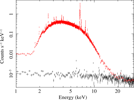
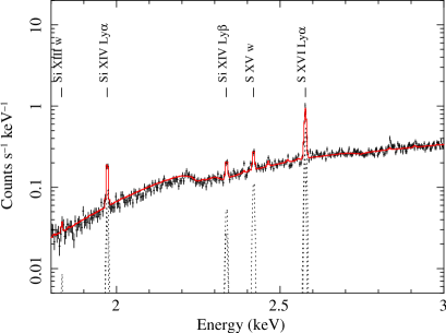
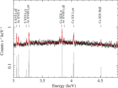
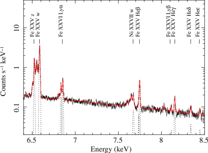
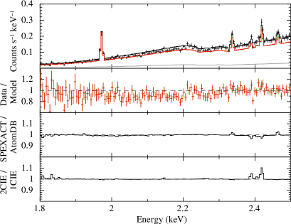
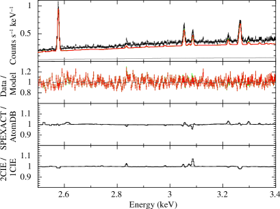
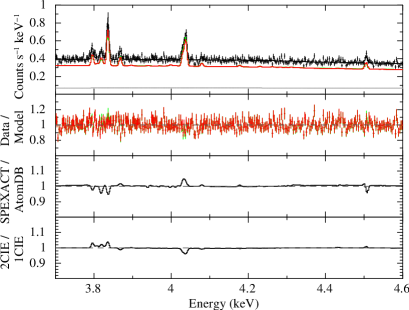
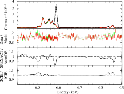
Figure 3 shows the spectra extracted from the Entire core region, focusing on the 1.8–3.0 keV, 3.0–4.8 keV, and 6.4–8.5 keV bands. Both He$\alpha$ and Ly$\alpha$ emission lines of Si, S, Ar, Ca, and Fe were detected and resolved. Furthermore, some transitions from higher principal quantum numbers are also resolved; up to $\epsilon$ ($n=6$) from Fe in particular.

In order to derive the observed fluxes of these lines, we fitted the spectra in the three energy bands listed above with a phenomenological model consisting of continuum emission and Gaussian lines. We used a CIE plasma model based on AtomDB (the apec model) in which the strong lines listed in Table 3.1 were replaced with Gaussians. In accordance with the First paper, the metal abundance of the plasma model was fixed at 0.62 solar and the line-of-sight velocity dispersion was fixed at 146 km s^-1 to represent weaker emission lines not listed in Table 3.1. Even when these parameters are varied by $\pm$20% (much higher than statistical errors shown in the Z paper and the V paper), there is no significant impact on our line flux measurements. Doublets of the Lyman series were not resolved except for Fe XXVI Ly$\alpha$, and hence their centroid energies, line widths, and flux ratios were tied as shown in Table 3.1. The line centroids and widths for Fe XXV He$\beta_{1}$ and Fe XXV He$\beta_{2}$ were also tied as described in Table 3.1. Unresolved structures in Ca XIX He$\beta$, Fe XXV He$\gamma$, Fe XXV He$\delta$, and Fe XXV He$\epsilon$ were represented by single Gaussians. The Gaussian fluxes we obtained are shown in Table 3.1. The results of the line centroids and width, though not relevant to our analysis, are summarized in Appendix B. Readers are referred to the V paper for a detailed discussion of the velocity dispersions and line-of-sight velocity shifts.

Figure 4: Upper 8 panels show flux ratios of the emission lines as a function of the excitation temperature, calculated from AtomDB (black solid curve) and SPEXACT (gray dashed curve) assuming a single temperature CIE plasma. The lines used in the calculations are denoted in each panel. The color boxes show the ranges of the observed line ratios and the corresponding AtomDB temperatures at the1$\sigma$ confidence level. Magenta, blue, cyan, and green correspond to the Entire core, Rim, Nebula, and Outer regions, respectively. When the ranges of the statistical errors of the observed line ratios are outside the models, 3$\sigma$ lower limits are shown instead by the color arrows. Lower 9 panels are the same as the upper panels but for the ionization temperature.

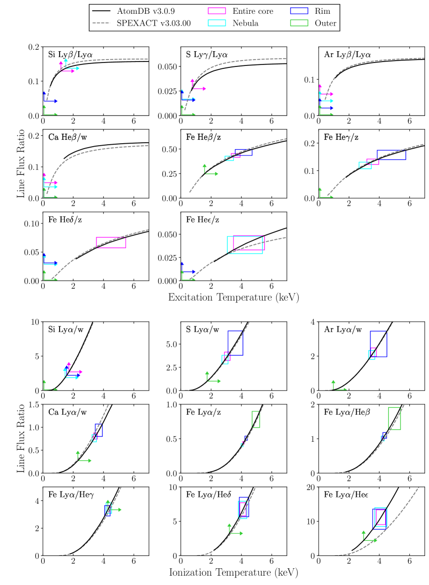
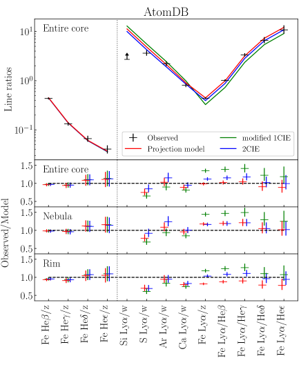
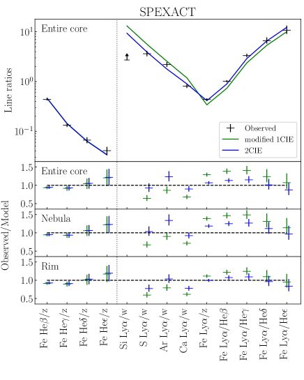
Assuming a single-temperature CIE plasma, and employing the AtomDB and SPEXACT databases, we calculated how the line ratios considered here depend on the temperature. The calculated temperature dependencies are shown in Figure 4. Line emissivities used in these calculations are given in Appendix C along with measurements of emission measure based on single line fluxes. Except for He$\epsilon$/z and Ly$\alpha$/He$\epsilon$ ratios, the two codes gave consistent values with each other within 5–10% for the interesting temperature range, 1–7 keV. Detailed comparisons of line emissivities between the two codes are discussed in the Atomic paper.

A line ratio of different transitions in the same ion reflects the kinetic temperature of free electrons in the plasma, and is referred to as “excitation temperature” or $T_{\mathrm{e}}$. Referring to Figure 4, we calculated the $T_{\mathrm{e}}$ from the observed line ratios of Ly$\beta$/Ly$\alpha$ of Si and Ar, Ly$\gamma$/Ly$\alpha$ of S, He$\beta$/w of Ca, and He$\beta$/z, He$\gamma$/z, He$\delta$/z, and He$\epsilon$/z of Fe (top three rows of Figure 4). S Ly$\beta$ is not used because it is not separated from Ar z, whose energy is 3102 eV (see Figure 3). Fe Ly$\beta$ is not used because of the low observed flux. Fluxes of Ly$\alpha_{1}$ and Ly$\alpha_{2}$ were co-added in this calculation. In the same manner, the fine structures of Ly$\beta$, Ly$\gamma$, He$\beta$, He$\gamma$, He$\delta$ and He$\epsilon$ were also summed. The interval of the observed line ratios and the corresponding temperature ranges are overlaid on Figure 4 as color boxes.

Separately from the $T_{\mathrm{e}}$ diagnostics, we used line ratios of different ionization species to measure the ion fraction for each element. We parameterize these ratios by “ionization temperatures” or $T_{\mathrm{Z}}$. When the emission comes from a single component and optically thin plasma under the CIE, $T_{\mathrm{Z}}$ from every element should be the same as $T_{\mathrm{e}}$. The $T_{\mathrm{Z}}$ were calculated using the line ratios of Ly$\alpha$/w of Si, S, Ar, and Ca and Ly$\alpha$/z, Ly$\alpha$/He$\beta$, Ly$\alpha$/He$\gamma$, Ly$\alpha$/He$\delta$, and Ly$\alpha$/He$\epsilon$ of Fe (bottom three rows of Figure 4). The temperature range derived from the observed line ratios are shown in Figure 4.

(a) Entire core

(b) Nebula

(c) Rim

(d) Outer

Figure 5: Excitation temperatures and ionization temperatures derived from individual line ratios in (a) the Entire core, (b) Nebula, (c) Rim, and (d) Outer regions. Cyan, green, orange, pink, and purple indicate Si, S, Ar, Ca, and Fe, respectively. The results based on AtomDB and SPEXACT are shown by the solid and dotted lines, respectively. The horizontal dash-dotted lines show the best-fit $kT_{\mathrm{line}}$ of the modified 1T model described in §3.2.1 and §3.3.

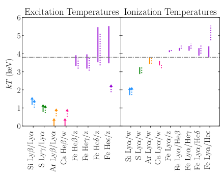
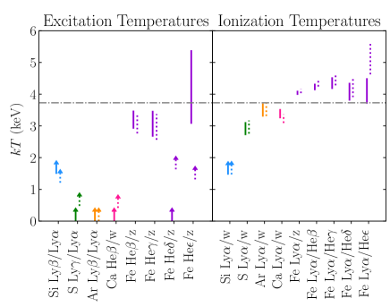
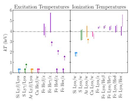
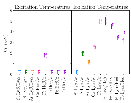
We summarize the derived $T_{\mathrm{e}}$ and $T_{\mathrm{Z}}$ in Figure 5. $T_{\mathrm{Z}}$ from Fe, which is determined with the smallest statistical uncertainties, has typical values of 4–5 keV. $T_{\mathrm{Z}}$ from the Entire core and Nebula regions are clearly different among elements; namely there is a tendency of increasing $T_{\mathrm{Z}}$ with increasing atomic number. These results indicate deviation from a single temperature CIE model. $T_{\mathrm{Z}}$ from the Rim also suggests a slight deviation from a single temperature model. The results of the Outer region are consistent with a single temperature approximation.

$T_{\mathrm{e}}$ from Fe for the Nebula and Rim are about 3 and 4 keV, respectively. In the Nebula and Entire core regions, $T_{\mathrm{e}}$ from Fe are lower than $T_{\mathrm{Z}}$ at the 2–3 $\sigma$ level, providing further evidence for deviation from the single temperature approximation. For Si, S, Ar, and Ca, the line ratios which are sensitive to $T_{\mathrm{e}}$ are all consistent with the CIE prediction with the temperature of 2–4 keV within the statistical 1–2$\sigma$ errors, however, the corresponding $T_{\mathrm{e}}$ are not constrained.

3.2 Modelling of the Broad-band Spectrum in the Entire Core Region

We then tried to reproduce the broad-band (1.8–20.0 keV) spectrum with optically-thin thermal plasma models based on AtomDB and SPEXACT. In the analysis of this section, we focused on the spectrum of the Entire core region in order to ignore the contamination of photons scattered due to the point spread function (PSF) of the telescope, and to investigate uncertainties due to the atomic codes and the effective area calibration.

3.2.1 Single temperature plasma model

Best fit parameters for the Entire core region Model/Parameter AtomDB v3.0.9 SPEXACT v3.03.00 1CIE model      $kT_{\mathrm{1CIE}}$ (keV) 3.95${}^{+0.01}_{-0.01}$ 3.94${}^{+0.01}_{-0.01}$      $N$ (10¹² cm^-5) 23.20${}^{+0.05}_{-0.05}$ 22.78${}^{+0.04}_{-0.04}$      C-statistics/dof 13123.6/12979 13181.7/12979 Modified 1CIE model      $kT_{\mathrm{cont}}$ (keV) 4.01${}^{+0.01}_{-0.01}$ 3.95${}^{+0.01}_{-0.01}$      $kT_{\mathrm{line}}$ (keV) 3.80${}^{+0.02}_{-0.02}$ 3.89${}^{+0.02}_{-0.02}$      $N$ (10¹² cm^-5) 22.77${}^{+0.04}_{-0.04}$ 22.67${}^{+0.05}_{-0.05}$      C-statistics/dof 13085.9/12978 13178.7/12978 2CIE model (modified CIE + CIE)      $kT_{\mathrm{cont}1}$ (keV) 3.66${}^{+0.01}_{-0.02}$ 3.40${}^{+0.02}_{-0.01}$      $kT_{\mathrm{line}1}$ (keV) 3.06${}^{+0.04}_{-0.03}$ 2.92${}^{+0.03}_{-0.03}$      $kT_{2}$ (keV) 4.51${}^{+0.02}_{-0.03}$ 4.73${}^{+0.02}_{-0.02}$      $N_{1}$ (10¹² cm^-5) 12.98${}^{+0.05}_{-0.05}$ 13.27${}^{+0.13}_{-0.09}$      $N_{2}$ (10¹² cm^-5) 9.71${}^{+0.06}_{-0.05}$ 9.45${}^{+0.07}_{-0.05}$      C-statistics/dof 13058.5/12976 13093.9/12976 Power-law DEM model      index 10.92${}^{+0.11}_{-0.11}$ 4.68${}^{+0.03}_{-0.03}$      $kT_{\mathrm{max}}$ (keV) 4.01${}^{+0.06}_{-0.01}$ 4.29${}^{+0.01}_{-0.01}$      $N$ (10¹² cm^-5) 21.38${}^{+0.24}_{-0.24}$ 15.39${}^{+0.04}_{-0.04}$      C-statistics/dof 13123.4/12978 13147.6/12978 Gaussian DEM model      $kT_{\mathrm{mean}}$ (keV) 3.94${}^{+0.01}_{-0.01}$ 3.89${}^{+0.01}_{-0.01}$      $\sigma$ (keV) 0.60${}^{+0.08}_{-0.11}$ 1.01${}^{+0.05}_{-0.05}$      $N$ (10¹² cm^-5) 11.65${}^{+0.02}_{-0.02}$ 11.67${}^{+0.03}_{-0.03}$      C-statistics/dof 13121.1/12978 13138.7/12978

(a)

(b)

(c)

(d)

(e)

(f)

Figure 6: The spectra in the Entire core region fitted with the modified-1CIE model. The entire energy band of 1.8–20.0 keV is shown in (a), and narrower energy bands of 1.8–2.5 keV, 2.5–3.4 keV, 3.7–4.6 keV, 6.4–6.9 keV, and 7.5–8.5 keV are shown in (b)–(f). The black solid curve is the total model flux, and the red and gray curves indicate the ICM component based on AtomDB and the AGN component, respectively. (b)–(f) include the green lines indicating the ICM component based on SPEXACT. The figure (e), covering the 6.4–6.9 keV band, shows also the Gaussian (black dashed curve) which substitutes Fe XXV w in the plasma model. All the spectra are rebinned after the fitting just for display purposes. The second panels in (b)–(f) are the ratio of the data to the model of AtomDB (red) and SPEXACT (green). The third panels in (b)–(f) are the comparison of SPEXACT and AtomDB in the modified 1CIE model. The bottom panels in (b)–(f) shows the ratio of the 2CIE model to the modified 1CIE model based on AtomDB.

Figure 7: Comparison of the best-fit temperatures and C-statistics among different ARFs and atomic databases for the modified 1CIE model.

Although the SXS spectra indicate multi-temperature conditions, we begin by fitting the data with the simplest model, that is, a single temperature CIE plasma model (hereafter the 1CIE model), with the temperature ($kT_{\mathrm{1CIE}}$), the abundances of Si, S, Ar, Ca, Cr, Mn, Fe, and Ni, the line-of-sight velocity dispersion, and the normalization ($N$) as free parameters. The abundances of other elements from Li through Zn were tied to that of Fe. Since the resonance line of He-like Fe (Fe XXV w) is subject to the resonance scattering effect (see the RS paper), we replaced it by a single Gaussian so that it does not affect the parameters we obtained. The best-fit parameters are shown in Table 3.2.1; AtomDB and SPEXACT give consistent temperatures of $3.95\pm 0.01$ keV and $3.94\pm 0.01$ keV, respectively. The C-statistics are within the expected range that is calculated according to Kaastra (2017), and hence the fits are acceptable even in these simple models.

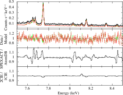
In the 1CIE fit, both the continuum shape and the emission-line fluxes participate in the temperature determination. In order to fully utilize the line resolving power of the SXS, we then modeled the continuum and lines separately and determined the continuum temperatures ($kT_{\mathrm{cont}}$) and the line temperatures ($kT_{\mathrm{line}}$) (hereafter the modified 1CIE model). In this model, $kT_{\mathrm{cont}}$ and $kT_{\mathrm{line}}$ were independently allowed to vary whereas the other parameters were common (implemented as the bvvtapec model in Xspec). The best-fit parameters we obtained are shown in Table 3.2.1. Both AtomDB and SPEXACT provide a reasonably good fit to the observed spectrum as shown in Figure 6. Compared to $kT_{\mathrm{1CIE}}$, $kT_{\mathrm{cont}}$ and $kT_{\mathrm{line}}$ become slightly higher and lower, respectively, for both AtomDB and SPEXACT. Since $kT_{\mathrm{cont}}$ is closer to $kT_{\mathrm{1CIE}}$ than $kT_{\mathrm{line}}$, the continuum shape most likely determines the temperature of the 1CIE model, rather than the line fluxes, even with high-resolution spectroscopy measurements. The temperature differences between AtomDB and SPEXACT are formally statistically significant, but are less than 0.1 keV.

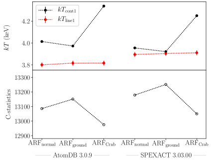
The difference between $kT_{\mathrm{cont}}$ and $kT_{\mathrm{line}}$ is at most 0.23 keV but statistically significant. As we found the multi-temperature structure from the line ratio diagnostics (§3.1), that difference is possible. However, an uncertainty in the effective area also might affects the results; the in-flight calibration of Hitomi was not completed because of its short life time. We therefore assessed this uncertainty using the modified ARF based on the ground telescope calibration (ARF_ground) and the actual Crab data (ARF_Crab). See Appendix D for the detailed correction method. We fitted the modified 1CIE model using ARF_ground and ARF_Crab. The correction of the ARF slightly affects the parameters of the AGN components as well (see Table 4 of the AGN paper). Even though the differences are very small, we used the specific AGN parameter values corresponding to each assumed ARF in our fits. The temperatures and C-statistics we obtained are summarized in Figure 7. $kT_{\mathrm{cont}}$ varies depending on ARF because the continuum shape is subject to the effective area shape. On the other hand, the values of $kT_{\mathrm{line}}$ measured with different assumptions for the ARF remain consistent with each other. Therefore, $kT_{\mathrm{line}}$ provides the most robust estimate of the temperature from the SXS spectrum assuming a single-phase model. In terms of the C-statistics, the ARF_Crab gives the best-fit, but this choice of ARF also results in the largest difference between $kT_{\mathrm{cont}}$ and $kT_{\mathrm{line}}$. This illustrates the difficulty of effective area calibration with the limited amount of available data.

Even though the AGN paper carefully modeled the AGN emission, the uncertainty of its model parameters and their impact on the best-fit temperature structure should also be considered. If the AGN model is slightly changed, $kT_{\mathrm{cont}}$ would again change, while $kT_{\mathrm{line}}$ would be less affected as demonstrated in the comparison of the ARFs.

3.2.2 Two temperature plasma models

Figure 8: Comparison of the best-fit temperatures and C-statistics among different ARFs and atomic databases for the 2CIE model.

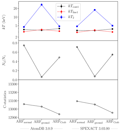
The line ratio diagnostics in §3.1 actually indicate the presence of multi-temperature structure in the Perseus cluster core. As a simple approximation of the deviations from a single thermal phase, we first used a two-temperature model where another CIE model was added to the modified 1CIE model (hereafter the 2CIE model). The free parameters of the additional CIE component were the temperature and the normalization, while the abundances and the line-of-sight velocity dispersion were tied to those of the primary component. The results are shown in Table 3.2.1. As expected, the C-statistics are significantly improved from those of the modified 1CIE model ($\Delta C=$ 30–91). However, as shown in the bottom panels of Figure 6 (b)–(f), the continuum is almost the same and the difference of line emissivities are at most 10$\%$ compared to the 1CIE model. The temperatures and normalizations obtained with the two spectral codes are in reasonably good agreement, although some differences are statistically significant. The dominant component now has a temperature of $kT_{\mathrm{line}}=3.06\pm 0.03$ keV from AtomDB, which is fully consistent with $kT_{\mathrm{line}}=3.06^{+0.03}_{-0.08}$ keV from SPEXACT. The second thermal component is from hotter gas with $kT_{2}\sim 5$ keV; for this component, SPEXACT gives a $\sim 10$% higher temperature than AtomDB, and a somewhat lower relative normalization ($N_{2}/(N_{1}+N_{2})$ of 31% with SPEXACT and 43% with AtomDB). The temperatures derived from the 2CIE fit are consistent with the line ratio diagnostics shown in Figure 5; the ionization temperature of S is $\sim 3$ keV and that of Fe is $\sim 4.5$ keV. We also checked difference of the line-of-sight velocity dispersion between the lower and higher temperature components, but no significant difference was found (see Appendix E for details).

In the same manner as for the modified 1CIE model (§3.2.1), we examined the effect of different ARFs (ARF_ground and ARF_Crab) for the 2CIE model. Figure 8 shows the resulting temperatures, the ratio of the normalizations ($N_{2}/N_{1}$), and the C-statistics for each ARF. The best-fit parameter values vary significantly depending on the choice of ARF, but the temperatures of ARF_normal and ARF_Crab are very close to each other ($\sim$3 keV plus $\sim$5 keV). Only ARF_ground shows the presence of a $>$20 keV component, which seems physically less well motivated. The different trend in ARF_ground is likely caused by an incomplete modeling of the continuum; as shown in the middle panel of Figure 16 (Appendix D), downward convex residuals are seen in the 2–7 keV band for ARF_ground. In any case, the trend where the dominant component has a temperature of 3–4 keV and the sub-dominant additional phase has a higher temperature, is robust.

3.2.3 Other combinations of collisional plasma models

We also tried to add one more CIE component to the 2CIE model (i.e., 3CIE model), but no significant improvements of the C-statistics are found. Therefore, the 2CIE model is sufficient to reproduce the observed spectrum.

The actual temperature structure of the ICM might not consist of discrete temperature components but rather of a continuous temperature distribution. Indeed, some hints of a power-law or a Gaussian temperature distributions were reported in the literature (e.g., Kaastra et al. (2004); Simionescu et al. (2009)). We therefore applied these simple differential emission measure (DEM) models to the SXS spectrum. The emission measure profile, $EM(kT)$, is proportional to $(kT/kT_{\mathrm{max}})^{\alpha}$ for the power-law DEM model and to $\exp(-(kT-kT_{\mathrm{mean}})^{2}/2\sigma)$ for the Gaussian DEM model. The best-fit parameters of the models are summarized in Table 3.2.1. Both the power-law and the Gaussian DEM models show steep temperature distributions peaked at $\sim 4$ keV, even though the distributions based on SPEXACT are slightly wider (smaller index or larger $\sigma$) than those based on AtomDB. In any case, we found no significant improvements from the 2CIE model. Further investigation of the multi-temperature model is shown in Section 3.4 and Figure 10.

Another possible cause of the deviation from a single temperature model shown in the line ratio diagnostics is the NEI state, which is often observed in supernova remnants. We thus tried to fit the spectrum with a NEI model (the possibilities of both an ionizing and a recombining plasma are considered). However, the obtained ionization parameter becomes $nt>1\times 10^{12}$ cm^-3 s^-1, and the temperature is almost the same as the 1T model; therefore the model is consistent with a CIE state, and we find no significant signature of the NEI.

3.3 Spatial Variation of the Temperature Structure

Best fit parameters for Neubla, Rim and Outer Model/Parameter AtomDB v3.0.9 SPEXACT v3.03.00 Nebula Rim Outer Nebula Rim Outer Modified 1CIE model $kT_{\mathrm{cont}}$ (keV) 3.96${}^{+0.01}_{-0.01}$ 4.02${}^{+0.01}_{-0.01}$ 4.93${}^{+0.10}_{-0.10}$ 3.90${}^{+0.02}_{-0.02}$ 3.97${}^{+0.01}_{-0.01}$ 4.85${}^{+0.09}_{-0.09}$ $kT_{\mathrm{line}}$ (keV) 3.73${}^{+0.03}_{-0.03}$ 3.94${}^{+0.04}_{-0.04}$ 4.83${}^{+0.15}_{-0.16}$ 3.82${}^{+0.03}_{-0.07}$ 4.07${}^{+0.04}_{-0.04}$ 4.97${}^{+0.16}_{-0.14}$ $N$ (10¹² cm^-5) 14.75${}^{+0.05}_{-0.05}$ 15.31${}^{+0.04}_{-0.04}$ 5.22${}^{+0.10}_{-0.11}$ 14.68${}^{+0.08}_{-0.08}$ 15.23${}^{+0.04}_{-0.04}$ 5.21${}^{+0.09}_{-0.09}$      C-statistics/dof 11948.0/12200 10168.9/10300 6323.8/6929 12013.0/12200 10188.6/10300 6326.5/6929 2CIE model $kT_{\mathrm{cont}1}$ (keV) 3.56${}^{+0.42}_{-0.07}$ 3.65${}^{+0.02}_{-0.02}$ $\cdots$ 3.39${}^{+0.07}_{-0.09}$ 3.40${}^{+0.02}_{-0.02}$ $\cdots$ $kT_{\mathrm{line}1}$ (keV) 2.78${}^{+0.10}_{-0.37}$ 3.49${}^{+0.05}_{-0.05}$ $\cdots$ 2.60${}^{+0.24}_{-0.23}$ 3.27${}^{+0.05}_{-0.05}$ $\cdots$ $kT_{2}$ (keV) 4.32${}^{+0.02}_{-0.36}$ 4.98${}^{+0.05}_{-0.05}$ $\cdots$ 4.30${}^{+0.28}_{-0.16}$ 4.99${}^{+0.04}_{-0.03}$ $\cdots$ $N_{1}$ (10¹² cm^-5) 6.91${}^{+0.45}_{-3.40}$ 11.16${}^{+0.06}_{-0.06}$ $\cdots$ 6.24${}^{+2.14}_{-2.21}$ 9.94${}^{+0.06}_{-0.06}$ $\cdots$ $N_{2}$ (10¹² cm^-5) 7.73${}^{+3.46}_{-0.45}$ 4.28${}^{+0.04}_{-0.04}$ $\cdots$ 8.32${}^{+1.56}_{-1.97}$ 5.47${}^{+0.05}_{-0.05}$ $\cdots$      C-statistics/dof 11926.0/12198 10163.2/10298 $\cdots$ 11958.2/12198 10173.3/10298 $\cdots$ PSF corrected model $kT_{\mathrm{cont1}}$ (keV) 3.64${}^{+0.03}_{-0.03}$ 3.92${}^{+0.02}_{-0.02}$ 5.11${}^{+0.05}_{-0.05}$ 3.46${}^{+0.03}_{-0.03}$ 3.82${}^{+0.02}_{-0.02}$ 5.01${}^{+0.06}_{-0.05}$ $kT_{\mathrm{line1}}$ (keV) 2.68${}^{+0.04}_{-0.05}$ 3.88${}^{+0.05}_{-0.05}$ 5.00${}^{+0.16}_{-0.16}$ 2.66${}^{+0.04}_{-0.04}$ 3.97${}^{+0.06}_{-0.05}$ 5.19${}^{+0.17}_{-0.16}$ $kT_{2}$ (keV) 4.27${}^{+0.03}_{-0.03}$ 5.37${}^{+0.28}_{-0.30}$ $\cdots$ 4.53${}^{+0.03}_{-0.03}$ 6.80${}^{+0.56}_{-0.46}$ $\cdots$ $N_{1}$ (10¹² cm^-5) 5.54${}^{+0.04}_{-0.04}$ 10.18${}^{+0.05}_{-0.05}$ 4.51${}^{+0.04}_{-0.04}$ 6.63${}^{+0.05}_{-0.21}$ 10.35${}^{+0.05}_{-0.05}$ 4.52${}^{+0.04}_{-0.04}$ $N_{2}$ (10¹² cm^-5) 5.86${}^{+0.03}_{-0.04}$ 0.70${}^{+0.04}_{-0.03}$ $\cdots$ 4.72${}^{+0.04}_{-0.04}$ 0.52${}^{+0.04}_{-0.03}$ $\cdots$      C-statistics/dof 28404.6/29425 28444.1/29425

The fraction of integrated photons coming from each sky region. Sky regions Integrated regions Nebula Rim Outer Nebula 0.800 0.192 0.008 Rim 0.273 0.719 0.007 Outer 0.034 0.111 0.855

We next modeled the broad-band spectra in the Nebula, Rim, and Outer regions in order to look for spatial trends in the temperature distribution. The fit results obtained with the modified 1CIE model are shown in the top rows of Table 3.3. Compared to the result from the Entire core region, the temperature in the Nebula region is slightly lower, while that in the Rim region is slightly higher. The temperature continues to increase at larger radii, reaching 5 keV in the Outer region. These results are consistent with the temperature map obtained from XMM-Newton and Chandra observations (Churazov et al., 2003; Sanders & Fabian, 2007).

The line ratio diagnostics show a deviation from the single temperature approximation in the Nebula and Rim regions. We thus applied the 2CIE model to the spectra of those regions. The best-fit parameters are also shown in the middle rows of Table 3.3. The C-statistics were improved from the modified 1CIE model ($\Delta C=$ 6–59). Both the Nebula and Rim regions show the same composition as the Entire core (roughly 3 keV plus 5 keV), but with different normalization ratios (the relative contribution of the hotter component is lower in the Rim region, although significant differences between the two spectral codes are also found). Large asymmetrical errors of the normalizations in the Nebula region are likely due to the comparable normalization values of the two components and the limited energy band ($>1.8$ keV). In the Nebula region, the discrepancy between $kT_{\mathrm{cont}}$ and $kT_{\mathrm{line}}$ becomes large ($\sim$1.0 keV), and $kT_{\mathrm{line}}$ shows the lowest temperature of $\sim$2.7 keV among the different spatial regions considered. We also checked the 2CIE model in the Outer region, but no improvements from the modified 1CIE model were found ($\Delta C<1$), as expected from the line ratio diagnostics. The systematic uncertainty of the temperature measurements due to the different ARFs has a similar trend as the analysis of the Entire core region (see Appendix D).

The sizes of the regions used for spatially resolved spectroscopy are comparable to the angular resolution of the telescope. Therefore, photons scattered from the adjacent regions due to the telescope’s PSF tail might affect the fitting results. We calculated the expected fraction of scattered photons with ray-tracing simulations, and show the results in Table 3.3; the fractions reach up to 30%, and are not negligible. We thus performed a “PSF corrected” analysis, in which all the regions were simultaneously fitted taking into account the expected fluxes of photons scattered between regions. We used the 2CIE model for the Nebula and Rim regions and the 1 CIE model for the Outer region according to the results presented above. The best-fit parameters of the PSF corrected model are shown in the bottom rows of Table 3.3. After the PSF correction, the ratios of the normalizations are changed but the temperatures we obtained are almost consistent with those derived from the PSF “uncorrected” analysis.

3.4 Comparison with Multi-temperature Models from Previous Observations

(a)

(b)

(c)

(d)

Figure 9: Spectra fitted with the six-temperature model (upper panels) and ratios between the data and the model (lower panels). Left and right columns show the Hitomi/SXS and Chandra/ACIS spectra, respectively. The top and bottom rows correspond to the Nebula and Rim regions, respectively. The components included in the model are shown in color lines as denoted in each panel. The components whose normalizations are very low are not shown.

(a)

(b)

(c)

(d)

Figure 10: Normalization ratios of each temperature component derived from the multi-temperature models. The top rows are the results from AtomdB and the bottom rows are those from SPEXACT. The left and right columns correspond to Nebula and Rim, respectively. The red diamonds are Hitomi/SXS, the black circles are Chandra/ACIS, the gray circles are Chandra/ACIS of Sanders & Fabian (2007), and the blue squares are XMM-Newton/RGS. The results of XMM-Newton/RGS are shown only in the Nebula region because the RGS data does not cover the Rim region.

Surface brightness of the power-law component. Instrument AtomDB 3.0.9 SPEXACT 3.03.00 Nebula Rim Nebula Rim Hitomi/SXS $<$3.4 $<$1.2 $<1.8$ $<0.6$ Chandra/ACIS $6.3_{-0.5}^{+0.5}$ $2.0_{-0.3}^{+0.3}$ $6.6_{-0.5}^{+0.5}$ $1.9_{-0.3}^{+0.3}$ In the unit of 10${}^{-16}~{}$ erg cm^-2 s^-1 arcsec^-2 (2–10 keV band)

Chandra/ACIS and XMM-Newton/RGS observations revealed a multi-temperature structure ranging between 0.5–8.0 keV in the core of the Perseus cluster (Sanders & Fabian, 2007; Pinto et al., 2016). Here we use a similar multi-temperature analysis to check the consistency between Hitomi/SXS and these previous measurements.

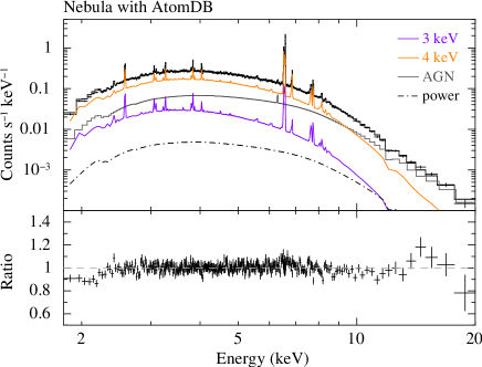
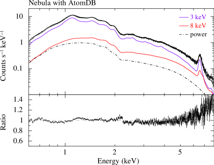
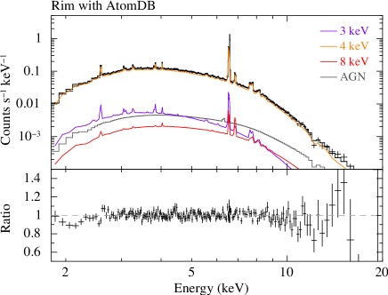
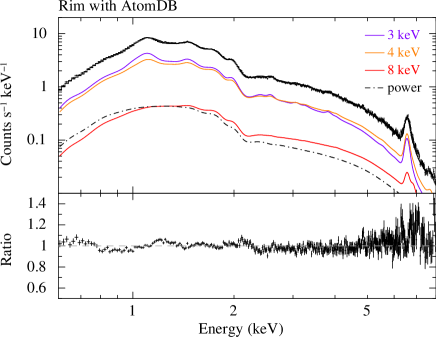
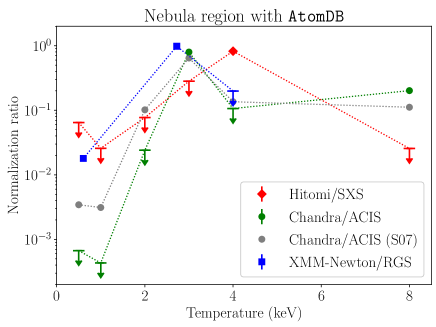
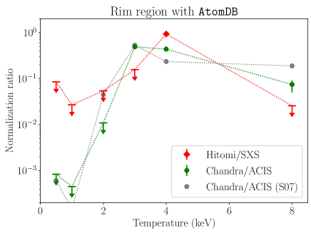
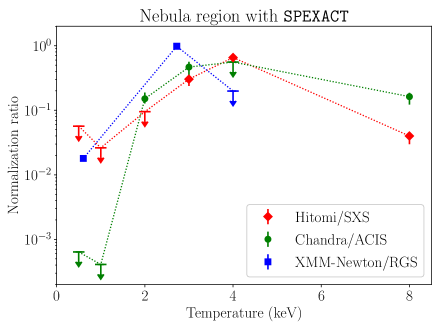
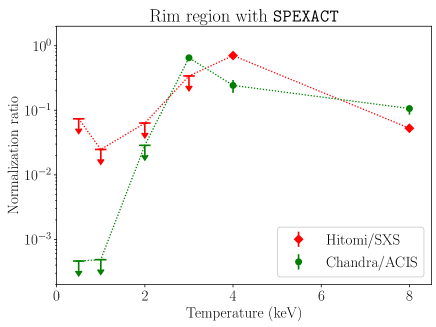
We fitted the SXS spectra extracted from the Nebula and Rim regions with a six-temperature CIE model consisting of 0.5 keV, 1 keV, 2 keV, 3 keV, 4 keV and 8 keV components following Sanders & Fabian (2007). The temperature of each component was fixed, and the abundance and line-of-sight velocity dispersion were common to all the components. The power-law component that was found in Sanders & Fabian (2007) and interpreted as a possible inverse-Compton emission was also included in our model with a fixed photon index of $\Gamma=2$. The spectra and the best-fit models in the Nebula and the Rim regions are shown in the left column of Figure 9. The normalizations we obtained for each temperature were scaled to sum to unity, and the results are plotted in Figure 10 as red diamonds. The profile of the scaled normalizations are very similar between AtomDB and SPEXACT, except for the 8 keV component which is detected with SPEXACT in both the Nebula and Rim regions while only its upper limit was obtained for AtomDB. The results indicate that the combination of the 3 keV, 4 keV, and 8 keV components approximates the 2CIE model obtained in §3.3 (roughly 3–4 keV plus 5 keV).

We also reanalyzed the Chandra/ACIS data because the effective area calibration was significantly improved during 2007–2009 (Nevalainen et al., 2010) and the atomic codes have been updated since the original work of Sanders & Fabian (2007). We fitted the spectra of the Nebula and Rim regions with the same six-temperature model as the SXS spectrum. The abundances and the velocity dispersion were fixed at the value obtained from the SXS analysis because Chandra’s energy resolution is not sufficient to determine these parameters. The AGN model was not included because we excluded the AGN from the ACIS spectral extraction region. When the absorption column density was fixed at $1.38\times 10^{21}$ cm^-2, we found a significant excess of the model over the data below 1 keV. We therefore allowed the absorption column density to vary to compensate for these residuals. The best-fit column density is $\sim 2.0\times 10^{21}$ cm^-2 for both the Nebula and Rim regions. The fitted spectra are shown in the right column of Figure 9. Large residuals can be seen above 5 keV in the Nebula region. Fitting these residuals with an additional power-law would require this to have a negative photon index. Therefore, we suspect these residuals are due to an instrumental effect rather than true astrophysical emission. The fact that no such residuals are seen in the SXS spectrum supports this inference. In addition, we see the wavy residuals in the entire energy band, which is probably due to the systematic uncertainty of the detector responses. The scaled normalizations we obtained are plotted in Figure 10 as black circles. The two spectral codes show similar trends, except for the 2 keV component in the Nebula region that is seen with SPEXACT but not with AtomDB.

Compared to the results of Sanders & Fabian (2007), our ACIS analysis shows a similar trend, but $\leq 2$ keV components are not detected (Figure 10). That is probably because the analysis of Sanders & Fabian (2007) used much smaller regions and could detect the lower temperature component that is concentrated in the cluster core and the filamentary structures. In the spectra of our analysis, which is taken from a much larger region, the lower temperature components could be smeared out by the dominant higher temperature component.

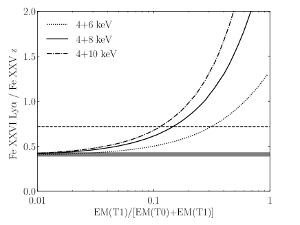
The Hitomi/SXS upper limits of the $\leq$2 keV components are consistent with the Chandra/ACIS results. However, the distribution of the higher temperature components seems somewhat different. The 4 keV component has the highest normalization in the SXS analysis, while the 3 keV component seems dominant in the ACIS fit. When the lower end of the energy band for the ACIS analysis was changed to 1.8 keV as same as the SXS analysis, we found that the peak of the normalization ratio became at 4 keV. It suggests that a derived normalization ratio of the ACIS analysis is affected by the fitted energy band, especially the band of Fe L-shell lines. The normalization of the 8 keV component for the SXS is lower than that for the ACIS by a factor of 2–10. To show sensitivity of the line ratio, Fe XXVI Ly$\alpha$/Fe XXV z, to the 8 keV component emission, we calculate the line ratio as a function of its fractional emission measure in Figure 11. The SXS observed line ratio ($\sim$0.4) and the expected line ratio derived from the best-fit ACIS multi-temperature model is also shown in the same figure. This indicates that the line flux of Fe XXVI Ly$\alpha$ primarily limits the hotter component emission. This SXS spectroscopic constraint is more robust and less dependent on the modeling of the continuum components, compared with previous continuum-based analysis.

Figure 11: The model line flux ratio of Fe XXVI Ly$\alpha$ to Fe XXV z as a function of the fractional emission measure of the secondary component in a two CIE model based on AtomDB. The temperature of the main component ($T0$) is 4.0 keV. The solid, dotted, and two dashed lines show the model for a second component with a temperature ($T1$) of 8.0, 6.0, and 10.0 keV, respectively. The ratio of SXS measurement in the Nebula region (0.41$\pm$0.02) is shown by the gray shaded area, and that of the Chandra model in the same region (0.8) is shown by the horizontal dashed line.

Although we employed this particular six-temperature model just to examine consistency with the Chandra result (Sanders & Fabian (2007), and our own analysis), we admit that the assumed six temperatures are not necessarily appropriate, because no emission measure is considered between the temperatures of 4 keV and 8 keV. This condition is inconsistent with the very likely presence of a component with $\sim 5$ keV temperature in the present SXS spectra, as indicated in Table 3.3 by the 2T fit to the Nebula and Rim spectra. In addition, the outer region of Perseus is known to have a typical temperature of 6–7 keV (e.g., Churazov et al. (2003)), and such a component must contribute to the SXS spectra at least due to projection. Given these, we repeated the multi-temperature fitting by adding a 7th component with its temperature fixed at 6 keV. As a result, the Nebula spectrum constrained the normalization (the same as in Figure 10) of this 6 keV component as $<0.05$ with AtomDB and $<0.13$ with SPEXACT, which are lower than those for the 4 keV emission. At the same time, the SXS normalization of the 8 keV component is $<0.03$ with AtomDB and $<0.07$ with SPEXACT, and is consistent with the six-temperature results. Therefore, the additional 6 keV component has no significant effect on the normalizations of the other temperature components.

The fluxes of the additional power-law component are shown in Table $*$ ‣ 3.4. The SXS detected no significant power-law component, while the ACIS data clearly require it in both the Nebula and Rim regions. These differences are discussed in §4.3.

The RGS data covers the energy band below 2 keV with high spectral resolution, and is complementary to the Hitomi/SXS data. Indeed, a very low temperature component with $kT<1$ keV was reported from the XMM-Newton/RGS observations (Pinto et al., 2016). Here, we fitted the RGS spectrum with a three-temperature plasma model by adding a fixed-temperature 4 keV component to the two-temperature model used in Pinto et al. (2016). For the RGS analysis, we have used the SPEX fitting package, because accounting for the line broadening due to the spatial extent of the source is not easily implemented in Xspec. A user model that calls Xspec externally and returns the model calculation to SPEX is used to implement fitting the RGS data with AtomDB.

The obtained best-fit temperatures are $0.60_{-0.02}^{+0.02}$ keV and $2.7_{-0.05}^{+0.08}$ keV for AtomDB and $0.55_{-0.06}^{+0.03}$ keV and $2.4_{-0.10}^{+0.08}$ keV for SPEXACT. The relative normalizations of each component are over-plotted on Figure 10. The profile peaks at $kT\sim 2.5$ keV, lower than both Chandra and Hitomi, and gives a significant detection of gas with $kT\sim 0.6$ keV. The normalization of this low temperature component measured with RGS is consistent with the Hitomi, but not with the Chandra upper limits for the 0.5 keV gas included in the six-temperature model; the upper limits for the 4 keV gas in both RGS and Chandra are lower than the Hitomi measurement for this temperature.

A simultaneous fitting of the SXS, ACIS, and RGS might provide a more complete picture of the temperature distribution. However, cross-instruments issues, such as the different spectral extraction regions and cross calibration of the effective areas, require more detailed analysis on the systematic errors. We therefore consider such analysis as a future work.

4 Discussion

4.1 Origin of the Deviations from a Single-temperature Model

(a)

(b)

Figure 12: Comparison between the observed line ratios (black crosses), the modified 1CIE model (green line), the 2CIE model (blue line), and the projection model (red line). The left and right figures show the calculations based on AtomDB and SPEXACT, respectively. The projection model is not shown in the right (SPEXACT) figure. The lower sub-panels show the ratios of the observation to the model in the Entire core, Nebula, and Rim regions from top thorough bottom. The vertical dotted line in the panels separates the ratios measuring the excitation temperature (left side) and the ionization temperature (right side).

The line ratio diagnostics presented in §3.1 show that, with the exception of the Outer region, the derived ionization temperatures are different for each element (Figure 5), and indicate multi-temperature structure.

In §3.2, we modeled the spectrum of the Entire core, Nebula, and Rim regions with single- and two-temperature plasma models. In Figure 12, we compare the observed line ratios and the line ratios predicted by the modified 1CIE and the 2CIE models, in order to investigate how these model approximations are able to reproduce the observations, and where the biggest discrepancies are found. This figure includes not only the line ratios that allow us to estimate the ionization temperatures, but also those sensitive to the excitation temperatures (Fe He$\beta$/z, He$\gamma$/z, He$\delta$/z, and He$\epsilon$/z). As expected from the C-statistics shown in Table 3.2.1 and Table 3.3, the line ratios of the 2CIE models are closer to the observed ones than those of the modified 1CIE models in all the region and in both AtomDB and SPEXACT. We then calculate chi-squared values ($\chi^{2}$) of the 2CIE models with respect to the observed line ratios in the Entire core region. The results are 22.0 and 19.6 in AtomDB and SPEXACT, respectively for 12 considered line ratio measurements. The major line ratios are reproduced better by the 2CIE model of SPEXACT, even though the broad-band fitting with the 2CIE model gives larger C-statistics in SPEXACT than AtomDB (Table 3.2.1).

One of the physical origins of the multi-temperature structure is the projection effect; the radial temperature gradient from the core to the outskirts is accumulated along the line of sight. In order to check this possibility, we used the azimuthally-averaged radial profiles of the temperature, density, and abundances derived from the de-projection analysis of the Chandra data using AtomDB (see Figure 7 in the RS paper). In this radial profile model, the temperatures vary from 3 keV to 6.5 keV with increasing radius from the cluster center in the range of 3–1000 kpc. We integrated this model along the line of sight and calculated the model line ratios shown in red in Figure 12 (left). The projection model of SPEXACT is not shown because the radial profile is derived based on AtomDB. In the Entire core region, $\chi^{2}$ of the projection model is 13.0, and is considerably better than that of the 2CIE model ($\chi^{2}=22.0$). On the other hand, in the Nebula and Rim regions, the projection model is almost the same or even worse compared to the 2CIE model. Azimuthal variation in temperature is probably significant in the Nebula and Rim regions as observed with Chandra (e.g., Fabian et al. (2011)), and this likely causes the difference from the projection model that is based on the azimuthally averaged radial profile.

A configuration in which the two temperature components determined from the 2CIE model are truly co-spatial cannot be ruled out. However, the derived temperatures in the 2CIE model ($\sim 3$ keV plus $\sim 5$ keV) are very close to the temperatures observed in the cluster center and outer. Therefore, the projection effect naturally explains the observed trend of lower ionization temperatures for ions with lower atomic number. As the equivalent widths of spectral lines from lighter elements are generally larger for lower temperatures, in the presence of a radial gradient along the line of sight, the emission-measure weighted average fluxes of these lines will naturally be biased towards the cooler gas, while the emission-measure weighted average fluxes of elements with higher atomic numbers will be biased towards values more typical of the hotter gas.

The low-temperature gas components ($kT<3$ keV) reported in previous Chandra and XMM-Newton observations are not seen in Figure 12. That is simply because the Hitomi/SXS energy band is restricted to energies above 1.8 keV and so is not sensitive to such low-temperature components; the derived upper limits from Hitomi for these thermal phases are not in conflict with previous results.

4.2 Uncertainties in Modeling the Multi-temperature Plasma

In §3.4, we compared the Hitomi/SXS results with the Chandra/ACIS and the XMM-Newton/RGS results. The best-fit emission measure distribution as a function of temperature is different among instruments (Figure 10): the normalization peaks at temperatures of 4 keV, 3 keV, and 2 keV for the SXS, ACIS, and RGS, respectively. The uncertainty of the detector response also affects the results, as shown by the discrepancy of the 8 keV component in the Hitomi/SXS and Chandra/ACIS.

Even in the single- or two-temperature model, the best-fit parameters are sensitive to the effective area calibration as demonstrated in Figure 7, Figure 8, and Appendix D. In the single-temperature modeling, we can robustly determine temperatures using only the line fluxes. However, in the two-temperature modeling, it is difficult to determine both temperatures and normalizations exactly.

Furthermore, we found that a small change in the atomic code significantly affects the result. As shown in Appendix F, the AtomDB 3.0.8 gives the temperatures of 1.7 keV and 4.1 keV in the 2CIE model, which is completely different from the results based on AtomDB 3.0.9. The difference between the two codes is only the emissivity of the dielectric-recombination satellite lines that is significantly lower than that of the transitions in the He-like ions (w, x, y, and z).

Therefore, we demonstrated that quantifying deviations from a single temperature model is a complex problem. As Figure 6 shows, the spectral differences between a two-temperature model consisting of a mixture of 3 and 5 keV plasma and a single-temperature model with $kT=4$ keV are very small, and thus the results of the 2CIE fit are sensitive to a large number of factors. These factors include the analysis energy band, the energy resolution, the calibration of the effective area, and atomic codes. For accurate analysis of the multi-temperature, non-dispersive high-resolution spectroscopy, a broad spectral band (0.5–10 keV), as will be achieved by XARM and Athena, is necessary.

4.3 Upper Limit for the power-law component

The diffuse radio emission is thought to be generated by Synchrotron mechanism of relativistic energy electrons with a 0.1–10 $\mu$G magnetic field in the ICM (Brunetti & Jones, 2014). These electrons scatter the CMB photons via the inverse-Compton scattering, which allows us to investigate the magnetic field in the ICM (Ota, 2012). Based on an assumption that inverse-Compton emission is generated by the same population of relativistic electrons, the volume-integrated magnetic field strength can be derived from intensities/upper-limits of IC emission (Rybicki & Lightman, 1979).

Sanders & Fabian (2007) reported the detection of a diffuse power-law component in the core of the Perseus cluster, which was not confirmed by the XMM-Newton analysis (Molendi & Gastaldello, 2009). The corresponding surface brightness in the 2–10 keV band measured by Sanders & Fabian (2007) is $\sim 15\times 10^{-16}$ and $\sim 8\times 10^{-16}$ erg cm^-2 s^-1 arcsec^-2 in Nebula and Rim, respectively. Our reanalysis of the Chandra/ACIS data also suggests the presence of such a power-law component, but with observed fluxes lower by a factor of 2–4 in better agreement with the upper limit of $5\times 10^{-16}$ erg cm^-2 s^-1 arcsec^-2 reported by Molendi & Gastaldello (2009). That is likely caused by the update of the calibration database described in Nevalainen et al. (2010); the response for the higher energy band is improved and significantly reduces the flux in that energy band.

In contrast, the Hitomi/SXS results show upper limits for this power-law component that are significantly lower than the fluxes measured with Chandra/ACIS.. As shown in Figure 9, large systematic residuals are present above 5 keV in the Chandra spectra even after the update of the effective area calibration, and they likely bias the power-law fluxes. A similar discrepancy was also reported in the comparison with the XMM-Newton/EPIC results (Molendi & Gastaldello, 2009). Since the Hitomi/SXS covers a wider energy range up to 20 keV, the obtained upper limits would be robust at least in the Rim region, in which the level of the AGN contamination is low.

Assuming the power-law component is due to inverse-Compton scattering, we can estimate the strength of the magnetic field ($B$) as discussed in Sanders et al. (2005). Using the SXS upper limit of $<1.2\times 10^{-16}$ erg cm^-2 s^-1 arcsec² in the Rim region, we obtained the lower limit of $B>0.4$ $\mu$G. This value is consistent with the results of other observations performed at other wavelengths ($\sim$7–25 $\mu$G) as discussed in Molendi & Gastaldello (2009).

5 Conclusion

Compared to the intricate structures revealed by the deep Chandra image of the core of the Perseus Cluster (e.g, Fabian et al. (2011)), at first glance the high-quality Hitomi SXS spectra of this source, which are sensitive to the temperature range of $\gtrsim 3$ keV, present a surprisingly quiescent view: the velocity dispersions are rather small (the First paper, the V paper), the chemical composition is remarkably similar to the solar neighborhood (the Z paper), and the spectra between 1.8–20 keV are largely well approximated by a single temperature model. The diffuse power-law component reported from previous Chandra measurements is also not required by the Hitomi data.

We have resolved line emission from various ions. This provides the first direct measurements of the electron temperature and ionization degree separately from different transitions of He-like and H-like ions of Si, S, Ar, Ca, and Fe. Compared with previous temperature measurements mostly based on the continuum shape, the new diagnostics are more sensitive to excitation processes and plasma conditions. We found that all observed ratios are broadly consistent with the CIE approximation. However, there are two signs of small deviation from a single temperature model. Firstly there is a trend of increasing ionization temperature with increasing atomic mass, particularly in the Nebula (central) region and possibly also in the surrounding Rim region. Secondly, the excitation temperature from Fe ($\sim 3$ keV) is lower than the corresponding ionization temperature and than the electron temperature determined from the spectral continuum ($\sim 4$ keV) for the Nebula. In the Nebula and Rim regions, the best-fit two temperature models suggest a mix of roughly 3 and 5 keV plasma, both of which are expected to be present based on deprojected temperature profiles previously measured with Chandra. On the other hand, the Outer region, corresponding to the farthest observation from the cluster core performed by Hitomi, shows no significant deviation from single temperature. No additional third temperature component, Gaussian nor power-law DEM model, nor significant emission from non-equilibrium ionization plasma are required to describe the spectra.

Even though we can not rule out a true multi-phase structure in which different temperature components are co-spatial, the projection effect is a natural explanation for the observed deviations from single temperature.

Best-fit models of lower-resolution spectra that include the energy band below 2 keV and the RGS spectra seem to present a contrasting picture, requiring a multi-phase thermal structure that the Hitomi observations are currently not sensitive to. It is clear that the dominant thermal component in the spectral fit depends on the energy band observed, and that detectors able to cover simultaneously the emission lines from all phases of the ICM are needed in order for a reliable temperature structure to be pinned down. High-resolution, non-dispersive spectroscopy with XARM or Athena will thus be crucial in order to assess the origins and robustness of the multi-temperature structure reported by CCD studies, and verify to what extent the complexity of cluster cores revealed by high-spatial resolution images corresponds to an equally complex picture along the energy axis.

Author contributions

S. Nakashima led this study in data analysis and wrote the manuscript. K. Matsushita, A. Simionescu, and T. Tamura reviewed the manuscript fully. K. Sato and T. Tamura performed a cross-check of the Hitomi/SXS analysis. Y. Kato analyzed the Chandra/ACIS archival data. A. Simionescu and N. Werner performed the XMM-Newton/RGS analysis. M. Furukawa and K. Sato constructed the projection model and checked the effect of the resonance scattering. M. Bautz, H. Akamatsu, M. Tsujimoto, H. Yamaguchi, K. Makishima, C. Pinto, Y. Fukazawa, R. Mushotzky, and J. de Plaa provided valuable comments that improved the draft. S. Nakashima, K, Sato, K. Nakazawa, T. Okajima, and N. Yamasaki contributed to fabrication of the instruments and performed the in-orbit operation and calibration.

We are thankful for the support from the JSPS Core-to-Core Program. We acknowledge all the JAXA members who have contributed to the ASTRO-H (Hitomi) project. All U.S. members gratefully acknowledge support through the NASA Science Mission Directorate. Stanford and SLAC members acknowledge support via DoE contract to SLAC National Accelerator Laboratory DE-AC3-76SF00515. Part of this work was performed under the auspices of the U.S. DoE by LLNL under Contract DE-AC52-07NA27344. Support from the European Space Agency is gratefully acknowledged. French members acknowledge support from CNES, the Centre National d’Études Spatiales. SRON is supported by NWO, the Netherlands Organization for Scientific Research. Swiss team acknowledges support of the Swiss Secretariat for Education, Research and Innovation (SERI). The Canadian Space Agency is acknowledged for the support of Canadian members. We acknowledge support from JSPS/MEXT KAKENHI grant numbers 15J02737, 15H00773, 15H00785, 15H02090, 15H03639, 15H05438, 15K05107, 15K17610, 15K17657, 16J00548, 16J02333, 16H00949, 16H06342, 16K05295, 16K05296, 16K05300, 16K13787, 16K17672, 16K17673, 21659292, 23340055, 23340071, 23540280, 24105007, 24244014, 24540232, 25105516, 25109004, 25247028, 25287042, 25400236, 25800119, 26109506, 26220703, 26400228, 26610047, 26800102, JP15H02070, JP15H03641, JP15H03642, JP15H06896, JP16H03983, JP16K05296, JP16K05309, JP16K17667, and JP16K05296. The following NASA grants are acknowledged: NNX15AC76G, NNX15AE16G, NNX15AK71G, NNX15AU54G, NNX15AW94G, and NNG15PP48P to Eureka Scientific. H. Akamatsu acknowledges support of NWO via Veni grant. C. Done acknowledges STFC funding under grant ST/L00075X/1. A. Fabian and C. Pinto acknowledge ERC Advanced Grant 340442. P. Gandhi acknowledges JAXA International Top Young Fellowship and UK Science and Technology Funding Council (STFC) grant ST/J003697/2. Y. Ichinohe, K. Nobukawa, and H. Seta are supported by the Research Fellow of JSPS for Young Scientists. N. Kawai is supported by the Grant-in-Aid for Scientific Research on Innovative Areas “New Developments in Astrophysics Through Multi-Messenger Observations of Gravitational Wave Sources”. S. Kitamoto is partially supported by the MEXT Supported Program for the Strategic Research Foundation at Private Universities, 2014-2018. B. McNamara and S. Safi-Harb acknowledge support from NSERC. T. Dotani, T. Takahashi, T. Tamagawa, M. Tsujimoto and Y. Uchiyama acknowledge support from the Grant-in-Aid for Scientific Research on Innovative Areas “Nuclear Matter in Neutron Stars Investigated by Experiments and Astronomical Observations”. N. Werner is supported by the Lendület LP2016-11 grant from the Hungarian Academy of Sciences. D. Wilkins is supported by NASA through Einstein Fellowship grant number PF6-170160, awarded by the Chandra X-ray Center, operated by the Smithsonian Astrophysical Observatory for NASA under contract NAS8-03060.

We are grateful for contributions by many companies, including in particular, NEC, Mitsubishi Heavy Industries, Sumitomo Heavy Industries, and Japan Aviation Electronics Industry. Finally, we acknowledge strong support from the following engineers. JAXA/ISAS: Chris Baluta, Nobutaka Bando, Atsushi Harayama, Kazuyuki Hirose, Kosei Ishimura, Naoko Iwata, Taro Kawano, Shigeo Kawasaki, Kenji Minesugi, Chikara Natsukari, Hiroyuki Ogawa, Mina Ogawa, Masayuki Ohta, Tsuyoshi Okazaki, Shin-ichiro Sakai, Yasuko Shibano, Maki Shida, Takanobu Shimada, Atsushi Wada, Takahiro Yamada; JAXA/TKSC: Atsushi Okamoto, Yoichi Sato, Keisuke Shinozaki, Hiroyuki Sugita; Chubu U: Yoshiharu Namba; Ehime U: Keiji Ogi; Kochi U of Technology: Tatsuro Kosaka; Miyazaki U: Yusuke Nishioka; Nagoya U: Housei Nagano; NASA/GSFC: Thomas Bialas, Kevin Boyce, Edgar Canavan, Michael DiPirro, Mark Kimball, Candace Masters, Daniel Mcguinness, Joseph Miko, Theodore Muench, James Pontius, Peter Shirron, Cynthia Simmons, Gary Sneiderman, Tomomi Watanabe; ADNET Systems: Michael Witthoeft, Kristin Rutkowski, Robert S. Hill, Joseph Eggen; Wyle Information Systems: Andrew Sargent, Michael Dutka; Noqsi Aerospace Ltd: John Doty; Stanford U/KIPAC: Makoto Asai, Kirk Gilmore; ESA (Netherlands): Chris Jewell; SRON: Daniel Haas, Martin Frericks, Philippe Laubert, Paul Lowes; U of Geneva: Philipp Azzarello; CSA: Alex Koujelev, Franco Moroso.

Appendix A Gain Correction

We checked uncertainties of the gain scale of the SXS and corrected them using the Perseus data themselves, because the gain scale calibration is limited due to the short life of Hitomi. The procedure described in this section is essentially the same as that used in the Z paper and Atomic paper, except that the reference redshift was changed from 0.01756 to 0.017284 according to the V paper.

We first applied a linear gain shift for each pixel in each observation so that the apparent energies of the Fe XXV lines agree with a redshift of 0.017284. The resulting amount of the energy shift at 6.5 keV is 1.0$\pm$1.9 eV (mean and standard deviation). This pixel-by-pixel redshift correction removes not only the remaining gain errors among pixels but also the spatial variation of the Doppler shift for the ICM. Our results are not affected by this possible “over-correction”.

We then co-added spectra of all the pixels for each observation and investigated the energy shifts of each line in the 1.8–9.0 keV band. Figure 13 summarizes the differences of line energies from the fiducial values assuming a redshift of 0.017284. We modeled these data by the parabolic function shown below, in which $\Delta E$ at $E=6586.5$ eV was constrained to zero:

$$E_{\rm cor}=E+a\times(E-6586.5)+b\times(E-6586.5)^{2}{\rm\;eV}.$$ (1)

The obtained parameters are

$$a =-4.888\times 10^{-4} {\rm\;and\;}b=2.035\times 10^{-6},$$ (2)

$$a =4.303\times 10^{-4} {\rm\;and\;}b=2.390\times 10^{-4},$$ (3)

$$a =6.250\times 10^{-4} {\rm\;and\;}b=2.702\times 10^{-4},$$ (4)

$$a =8.640\times 10^{-4} {\rm\;and\;}b=3.439\times 10^{-4},$$ (5)

for obs1, obs2, obs3, and obs4, respectively. We applied these corrections to all the pixels. As confirmed in Figure 6 of the RS paper, these gain corrections have no impact on the line flux measurement, which is crucial for the temperature measurements.

(a) obs1

(b) obs2

(c) obs3

(d) obs4

Figure 13: Parabolic functions for the gain correction in each observation.

Appendix B Detailed best-fit parameters of the Gaussian fits

The centers and widths derived from the Gaussian fits in §3.1 are shown in Table B. The obtained line widths are consistent with the results described in V paper.

Observed line centers and widths derived from the Gaussian fits.. Line name $E_{0}$ (eV) Center (eV) Width (eV) Entire Core Nebula Rim Outer Entire Core Nebula Rim Outer Si XIII w 1865.0 1864.5${}^{+1.1}_{-1.0}$ 1864.3${}^{+1.9}_{-0.9}$ (fixed) (fixed) $<$1.7 $<$1.7 (tied) (tied) Si XIV Ly$\alpha_{1}$ 2006.1 2006.4${}^{+0.3}_{-0.2}$ 2006.5${}^{+0.3}_{-0.2}$ 2006.4${}^{+0.4}_{-0.3}$ 2006.5${}^{+1.2}_{-1.3}$ 1.4${}^{+0.3}_{-0.3}$ $<$1.5 1.7${}^{+0.5}_{-0.5}$ $<$2.9 Si XIV Ly$\beta_{1}$ 2376.6 2376.5${}^{+0.5}_{-0.5}$ 2376.2${}^{+0.5}_{-0.5}$ 2377.8${}^{+1.3}_{-1.4}$ 2378.5${}^{+1.1}_{-1.3}$ 2.4${}^{+0.5}_{-0.5}$ 2.2${}^{+0.5}_{-0.5}$ 3.8${}^{+1.3}_{-1.2}$ $<$2.0 S XV w 2460.6 2460.7${}^{+0.5}_{-0.3}$ 2460.6${}^{+0.6}_{-0.4}$ 2460.7${}^{+0.8}_{-0.6}$ (fixed) 2.2${}^{+0.6}_{-0.6}$ 2.6${}^{+0.8}_{-0.7}$ $<$2.2 (tied) S XVI Ly$\alpha_{1}$ 2622.7 2622.6${}^{+0.1}_{-0.1}$ 2622.7${}^{+0.1}_{-0.2}$ 2622.6${}^{+0.2}_{-0.2}$ 2621.6${}^{+0.9}_{-0.9}$ 1.8${}^{+0.2}_{-0.2}$ 1.9${}^{+0.2}_{-0.2}$ 1.7${}^{+0.3}_{-0.3}$ 2.0${}^{+1.0}_{-1.2}$ S XVI Ly$\beta_{1}$ 3106.7 3106.4${}^{+0.3}_{-0.3}$ 3106.0${}^{+0.4}_{-0.4}$ 3107.0${}^{+0.3}_{-0.5}$ 3116.1${}^{+0.7}_{-1.3}$ 2.1${}^{+0.4}_{-0.3}$ 2.4${}^{+0.5}_{-0.4}$ 1.8${}^{+0.5}_{-0.7}$ $<$1.8 S XVI Ly$\gamma_{1}$ 3276.3 3276.8${}^{+0.3}_{-0.8}$ 3276.7${}^{+0.5}_{-0.8}$ 3276.3${}^{+1.0}_{-0.8}$ 3275.7${}^{+1.4}_{-1.4}$ $<$2.0 $<$2.1 1.8${}^{+1.2}_{-1.4}$ $<$2.4 Ar XVII w 3139.6 3139.5${}^{+0.3}_{-0.3}$ 3139.5${}^{+0.3}_{-0.4}$ 3139.3${}^{+1.2}_{-1.1}$ 3142.4${}^{+0.8}_{-1.0}$ 1.5${}^{+0.4}_{-0.4}$ 1.1${}^{+0.5}_{-0.6}$ 3.0${}^{+1.4}_{-1.1}$ $<$1.9 Ar XVIII Ly$\alpha_{1}$ 3323.0 3322.9${}^{+0.2}_{-0.3}$ 3323.1${}^{+0.3}_{-0.4}$ 3322.5${}^{+0.5}_{-0.4}$ 3326.6${}^{+2.2}_{-2.2}$ 2.7${}^{+0.4}_{-0.4}$ 3.0${}^{+0.4}_{-0.4}$ 2.2${}^{+0.6}_{-0.6}$ 4.1${}^{+2.3}_{-1.6}$ Ar XVIII Ly$\beta_{1}$ 3935.7 3935.0${}^{+0.9}_{-1.0}$ 3936.2${}^{+0.7}_{-1.3}$ 3931.4${}^{+1.5}_{-1.7}$ 3946.7${}^{+0.6}_{-1.2}$ 2.8${}^{+1.0}_{-0.8}$ 2.3${}^{+1.0}_{-0.9}$ 3.7${}^{+1.7}_{-1.6}$ $<$1.2 Ca XIX w 3902.4 3902.4${}^{+0.2}_{-0.2}$ 3902.5${}^{+0.2}_{-0.3}$ 3902.1${}^{+0.3}_{-0.4}$ 3902.4${}^{+1.5}_{-1.1}$ 2.3${}^{+0.2}_{-0.2}$ 2.4${}^{+0.3}_{-0.3}$ 2.2${}^{+0.4}_{-0.4}$ 2.7${}^{+1.5}_{-1.2}$ Ca XIX He$\beta_{1}$ 4583.5 4583.9${}^{+0.4}_{-0.9}$ 4583.8${}^{+0.2}_{-0.9}$ (fixed) (fixed) $<$1.6 $<$1.4 (tied) (tied) Ca XX Ly$\alpha_{1}$ 4107.5 4107.9${}^{+0.3}_{-0.5}$ 4107.1${}^{+0.7}_{-0.4}$ 4108.4${}^{+0.5}_{-0.6}$ 4113.1${}^{+1.8}_{-1.5}$ 2.6${}^{+0.4}_{-0.4}$ 2.9${}^{+0.5}_{-0.5}$ 2.4${}^{+0.7}_{-0.6}$ 3.0${}^{+2.1}_{-1.2}$ Fe XXV w 6700.4 6700.7${}^{+0.0}_{-0.1}$ 6700.7${}^{+0.1}_{-0.1}$ 6700.6${}^{+0.1}_{-0.1}$ 6701.9${}^{+0.4}_{-0.2}$ 4.2${}^{+0.1}_{-0.1}$ 4.3${}^{+0.1}_{-0.1}$ 4.0${}^{+0.1}_{-0.1}$ 4.3${}^{+0.2}_{-0.2}$ Fe XXV z 6636.6 6636.5${}^{+0.1}_{-0.1}$ 6636.4${}^{+0.2}_{-0.1}$ 6636.5${}^{+0.1}_{-0.2}$ 6637.5${}^{+0.5}_{-0.5}$ 3.4${}^{+0.1}_{-0.1}$ 3.6${}^{+0.1}_{-0.1}$ 3.2${}^{+0.2}_{-0.2}$ 3.9${}^{+0.5}_{-0.5}$ Fe XXV He$\beta_{1}$ 7881.5 7881.1${}^{+0.2}_{-0.2}$ 7881.3${}^{+0.3}_{-0.3}$ 7881.0${}^{+0.3}_{-0.3}$ 7882.6${}^{+0.5}_{-1.8}$ 4.2${}^{+0.2}_{-0.3}$ 3.8${}^{+0.3}_{-0.4}$ 4.4${}^{+0.3}_{-0.3}$ 5.0${}^{+0.9}_{-0.8}$ Fe XXV He$\beta_{2}$ 7872.0 (tied) (tied) (tied) (tied) (tied) (tied) (tied) (tied) Fe XXV He$\gamma_{1}$ 8295.5 8295.3${}^{+0.4}_{-0.6}$ 8295.5${}^{+0.7}_{-0.7}$ 8295.1${}^{+0.6}_{-1.1}$ (fixed) 5.0${}^{+0.5}_{-0.5}$ 4.6${}^{+0.7}_{-0.6}$ 5.6${}^{+0.8}_{-0.7}$ $<$0.0 Fe XXV He$\delta_{1}$ 8487.4 8484.9${}^{+1.4}_{-1.2}$ 8485.7${}^{+1.7}_{-1.7}$ 8483.1${}^{+2.1}_{-1.7}$ (fixed) 6.7${}^{+1.3}_{-1.0}$ 6.5${}^{+1.7}_{-1.3}$ 7.1${}^{+2.8}_{-1.6}$ $<$0.0 Fe XXV He$\epsilon_{1}$ 8588.5 8592.6${}^{+1.3}_{-1.4}$ 8592.6${}^{+1.0}_{-1.9}$ 8594.3${}^{+3.0}_{-3.0}$ (fixed) 4.8${}^{+1.2}_{-1.0}$ 3.8${}^{+1.4}_{-1.2}$ 7.8${}^{+3.5}_{-2.2}$ $<$0.0 Fe XXVI Ly$\alpha_{1}$ 6973.1 6973.6${}^{+0.1}_{-0.5}$ 6973.3${}^{+0.4}_{-0.4}$ 6973.6${}^{+0.2}_{-0.6}$ 6973.9${}^{+1.1}_{-1.6}$ 4.3${}^{+0.2}_{-0.2}$ 4.7${}^{+0.3}_{-0.3}$ 3.8${}^{+0.2}_{-0.4}$ 6.1${}^{+1.2}_{-0.9}$ Fe XXVI Ly$\alpha_{2}$ 6951.9 6952.8${}^{+0.3}_{-0.5}$ 6952.7${}^{+0.5}_{-0.8}$ 6952.6${}^{+0.5}_{-0.5}$ 6953.1${}^{+1.4}_{-1.9}$ (tied) (tied) (tied) (tied) Fe XXVI Ly$\beta_{1}$ 8252.6 8255.3${}^{+1.0}_{-1.3}$ 8254.6${}^{+1.5}_{-1.9}$ 8254.7${}^{+1.5}_{-0.5}$ 8247.3${}^{+2.8}_{-0.9}$ $<$3.6 3.0${}^{+2.2}_{-1.9}$ $<$1.6 $<$3.5 Ni XXVII w 7805.6 7806.9${}^{+0.9}_{-0.6}$ 7807.2${}^{+0.9}_{-0.8}$ 7806.2${}^{+1.5}_{-1.2}$ 7804.0${}^{+2.5}_{-4.1}$ 5.4${}^{+0.8}_{-0.7}$ 5.4${}^{+0.9}_{-0.8}$ 5.8${}^{+1.7}_{-1.4}$ 6.6${}^{+3.6}_{-2.3}$ The Ly$\alpha_{2}$ lines of Si, S, Ar, and Ca are not shown because all the paramters of them are tied to Ly$\alpha_{1}$ (see Table 3.1 for details).

Fiducial energies of the lines at the rest frame.

Appendix C Single-line based emission measure limits

(a)

(b)

Figure 14: (a) Line emissivities of strong transitions from AtomDB for a given emission measure and metal abundances. The solid and dashed lines show H-like and He-like transitions, respectively. (b) Emission measure limits calculated from the AtomDB CIE model and the observed fluxes from the entire core.

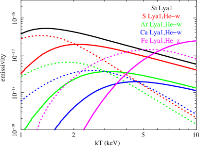
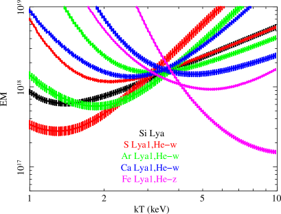
In Figure 14, we show theoretical emissivities for some of observed line transitions as a function of electron temperature based on AtomDB. The peak temperature, where the emissivity becomes maximum, from these ions cover a temperature range from 1.5 keV (H-like Si) to 13 keV (H-like Fe). Therefore measurements of line fluxes and ratios are sensitive to emission from plasma at around this temperature range.

Combined with these emissivity values, the observed flux for each transition (Table 3.1) provides constrains on emission measure for a given temperature and a metal abundance, as shown in Figure 14. If the line emission originate from a single component CIE plasma any two curves from a single element cross at a single point of the model temperature and emission measure. Furthermore, if the assumed metal abundances are correct, curves from different elements also cross at a single point. Our measured profiles from the entire core intersect together at around 3–4 keV, indicating that the observed line fluxes and hence their ratios can be approximated by a single component CIE plasma with the solar abundance ratios. From these curves we notice that the Fe XXVI Ly$\alpha$ is the most sensitive to hotter ($>4$ keV) emission and He-like S and Ar lines are the most sensitive to cooler ($<3$ keV) emission.

Appendix D Effective area uncertainties

Figure 15: Correction factor of the effective area with respect to the nominal value. The dot-dashed and solid lines indicate the calibration with the ground data and the actual Crab data, respectively.

Figure 16: Ratios of the Entire core spectrum to the best-fit modified 1CIE models with ARF_normal (top), ARF_ground (middle), and ARF_Crab (bottom).

Because of the short life time of Hitomi, its in-flight calibration plan is not completed. Data for the effective area calibration is especially limited. In order to assess the uncertainty of the effective area, two kind of evaluations have been performed as follows.

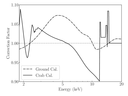
The instrument team compared the effective area derived from the ground calibration with that from ray-tracing simulations, and found residuals up to $\sim$7% depending on the incident photon energy (Figure 15). According to this investigation, the correction factor for the ARF is provided as an auxtransfile in CALDB. We corrected the ARF with this database (ARF_ground).

Tsujimoto et al. (2017) fitted the Crab spectrum with the canonical model ($\Gamma=2.1$; e.g., Madsen et al. (2015)), and found residuals up to $\sim$10% in the 1.8–20.0 keV band (Figure 15). The differences are probably due to uncertainties of not only the telescope reflectivity but also the transmission of the closed gate valve. This calibration method is not yet perfect because the spectral extraction region is smaller than that used for the canonical model due to the limited SXS FoV. Nevertheless, we made the local auxtransfile according to this result and corrected the ARF (ARF_Crab).

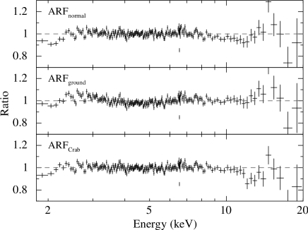
We made the corrected ARF based on the above corrections factors (ARF_ground and ARF_Crab). As described in §3.2.1, we fitted the spectrum of the Entire core region with the modified 1CIE model using these corrected ARFs. The residuals to the model with each ARF are shown in Figure 16. The best-fit temperatures and normalizations are summarized in Figure 7. We also fitted the spectrum with the 2CIE model in the same manner, and show the results in Figure 8.

In Figure 17 and Figure 18, we show the effect of the different ARFs on the fitting results for the Nebula, Rim, and (where applicable) Outer regions. Similarly to the Entire core region, the measured values of $kT_{\mathrm{line}}$ are consistent with each other, while those of $kT_{\mathrm{cont}}$ significantly vary among the ARFs. The 2CIE model in the Nebula region also shows a similar tendency with the Entire core region, with ARF_ground giving an unphysically high temperature of the second component, while the thermal structures inferred for the Rim region are consistent for all the assumed ARFs.

(a) Nebula

(b) Rim

(c) Outer

Figure 17: Fitting results of the modified 1CIE model with different ARFs in the Nebula, Rim, and Outer regions.

(a) Nebula

(b) Rim

Figure 18: Fitting results of the 2CIE model with different ARFs in the Nebula and Rim regions.

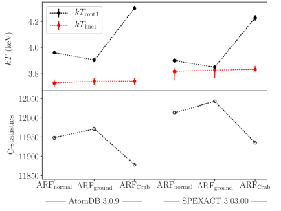
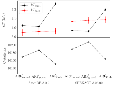
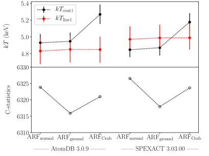
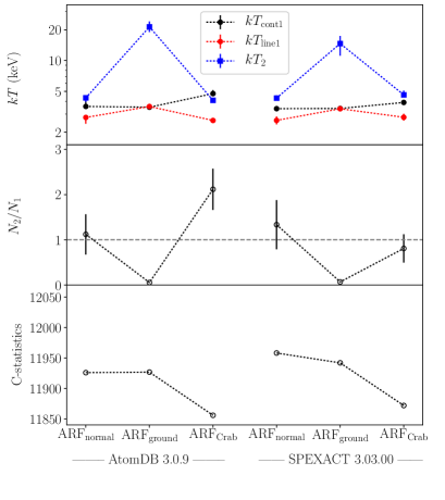
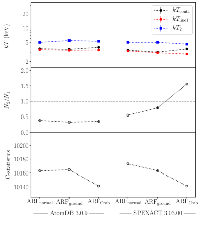
Appendix E Line-on-sight velocity dispersion in the 2CIE model

In the 2CIE model described in §3.2.2, the line-of-sight velocity dispersion is $145\pm 3$ km s^-1 and is consistent with the result of the single temperature model in the V paper. In order to investigate difference of the line-of-sight velocity dispersion between the lower and higher temperature components, we untied the link of the parameter between the two plasma models and refit the spectrum. As a result, the velocity dispersion of the lower and higher temperature components in SPEXACT are $130\pm 6$ km s^-1 and $210^{+47}_{-24}$ km s^-1, respectively, whereas those in AtomDB are both $145\pm 7$ km s^-1, suggesting that uncertainties of the atomic codes significantly affect the results. Therefore, we found no significant difference of the line-of-sight velocity dispersion between the different temperature components.

Appendix F Comparison between AtomDB versions 3.0.8 and 3.0.9

In the latest release of AtomDB (version 3.0.9), the emissivities of the dielectric-recombination satellite lines for highly charged Fe are changed with respect to version 3.0.8. The difference between versions 3.0.9 and 3.0.8 is shown in Figure 19. This difference does not appear to be large, but it significantly affects the result of the 2CIE model as shown in Table F. It demonstrates that uncertainties of the atomic code are very significant for the results obtained from high resolution spectroscopy measurements.

Figure 19: Comparison between AtomDB version 3.0.9 (red) and 3.0.8 (purple) with the same parameters. The top panel shows the SXS 6.47–6.63 keV spectrum in the Entire core region with the plasma models. The middle panel is the ratio of the data to the model. The bottom panel shows the ratio of the version 3.0.8 to the version 3.0.9.

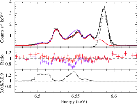
Comparsion of the best-fit parameters between AtomDB 3.0.9 and 3.0.8 Model/Parameter AtomDB v3.0.9 AtomDB v3.0.8 Modified 1CIE model      $kT_{\mathrm{cont}}$ (keV) 4.01${}^{+0.01}_{-0.01}$ 4.02${}^{+0.01}_{-0.01}$      $kT_{\mathrm{line}}$ (keV) 3.80${}^{+0.02}_{-0.02}$ 4.00${}^{+0.02}_{-0.02}$      $N$ (10¹² cm^-5) 22.77${}^{+0.04}_{-0.04}$ 23.07${}^{+0.04}_{-0.04}$      C-statistics/dof 13085.9/12978 13183.5/12978 2CIE model (modified CIE + CIE)      $kT_{\mathrm{cont}1}$ (keV) 3.66${}^{+0.01}_{-0.02}$ 4.06${}^{+0.01}_{-0.01}$      $kT_{\mathrm{line}1}$ (keV) 3.06${}^{+0.04}_{-0.03}$ 4.03${}^{+0.03}_{-0.08}$      $kT_{2}$ (keV) 4.51${}^{+0.02}_{-0.03}$ 1.59${}^{+0.03}_{-0.17}$      $N_{1}$ (10¹² cm^-5) 12.98${}^{+0.05}_{-0.05}$ 22.64${}^{+0.05}_{-0.05}$      $N_{2}$ (10¹² cm^-5) 9.71${}^{+0.06}_{-0.05}$ 0.68${}^{+0.11}_{-0.11}$      C-statistics/dof 13058.5/12976 13178.0/12976

References

- Akamatsu & Kawahara (2013) Akamatsu, H., & Kawahara, H. 2013, PASJ, 65, 16
- Arnaud (1996) Arnaud, K. A. 1996, in Astronomical Society of the Pacific Conference Series, Vol. 101, Astronomical Data Analysis Software and Systems V, ed. G. H. Jacoby & J. Barnes, 17
- Arnaud et al. (2010) Arnaud, M., Pratt, G. W., Piffaretti, R., et al. 2010, A&A, 517, A92
- Brunetti & Jones (2014) Brunetti, G., & Jones, T. W. 2014, International Journal of Modern Physics D, 23, 1430007
- Bulbul et al. (2014) Bulbul, E., Markevitch, M., Foster, A., et al. 2014, ApJ, 789, 13
- Cash (1979) Cash, W. 1979, ApJ, 228, 939
- Churazov et al. (2003) Churazov, E., Forman, W., Jones, C., & Böhringer, H. 2003, ApJ, 590, 225
- Conselice et al. (2001) Conselice, C. J., Gallagher, III, J. S., & Wyse, R. F. G. 2001, AJ, 122, 2281
- de Plaa et al. (2007) de Plaa, J., Werner, N., Bleeker, J. A. M., et al. 2007, A&A, 465, 345
- de Plaa et al. (2017) de Plaa, J., Kaastra, J. S., Werner, N., et al. 2017, ArXiv e-prints, arXiv:1707.05076
- Eckart et al. (2017) Eckart, M. E., Adams, J. S., Boyce, K. R., et al. 2017, Journal of Astronomical Telescopes, Instruments, and Systems
- Fabian et al. (2011) Fabian, A. C., Sanders, J. S., Allen, S. W., et al. 2011, MNRAS, 418, 2154
- Foster et al. (2012) Foster, A. R., Ji, L., Smith, R. K., & Brickhouse, N. S. 2012, ApJ, 756, 128
- Fujita et al. (2013) Fujita, Y., Kimura, S., & Ohira, Y. 2013, MNRAS, 432, 1434
- Fujita et al. (2008) Fujita, Y., Hayashida, K., Nagai, M., et al. 2008, PASJ, 60, 1133
- Fukazawa et al. (1994) Fukazawa, Y., Ohashi, T., Fabian, A. C., et al. 1994, PASJ, 46, L55
- Gu et al. (2012) Gu, L., Xu, H., Gu, J., et al. 2012, ApJ, 749, 186
- Gu et al. (2013) Gu, L., Gandhi, P., Inada, N., et al. 2013, ApJ, 767, 157
- Hitomi Collaboration (2016) Hitomi Collaboration. 2016, Nature, 535, 117
- Hitomi Collaboration (2017) —. 2017, ApJ, 837, L15
- Inoue et al. (2016) Inoue, S., Hayashida, K., Ueda, S., et al. 2016, PASJ, 68, S23
- Kaastra (2017) Kaastra, J. S. 2017, ArXiv e-prints, arXiv:1707.09202
- Kaastra et al. (1996) Kaastra, J. S., Mewe, R., & Nieuwenhuijzen, H. 1996, in UV and X-ray Spectroscopy of Astrophysical and Laboratory Plasmas, ed. K. Yamashita & T. Watanabe, 411–414
- Kaastra et al. (2004) Kaastra, J. S., Tamura, T., Peterson, J. R., et al. 2004, A&A, 413, 415
- Kalberla et al. (2005) Kalberla, P. M. W., Burton, W. B., Hartmann, D., et al. 2005, A&A, 440, 775
- Kilbourne et al. (2017) Kilbourne, C. A., Sawada, M., Tsujimoto, M., et al. 2017, PASJ
- Leccardi & Molendi (2008) Leccardi, A., & Molendi, S. 2008, A&A, 486, 359
- Madsen et al. (2015) Madsen, K. K., Reynolds, S., Harrison, F., et al. 2015, ApJ, 801, 66
- Makishima et al. (2001) Makishima, K., Ezawa, H., Fukuzawa, Y., et al. 2001, PASJ, 53, 401
- Markevitch & Vikhlinin (2007) Markevitch, M., & Vikhlinin, A. 2007, Phys. Rep., 443, 1
- Markevitch et al. (2000) Markevitch, M., Ponman, T. J., Nulsen, P. E. J., et al. 2000, ApJ, 541, 542
- Matsushita et al. (2002) Matsushita, K., Belsole, E., Finoguenov, A., & Böhringer, H. 2002, A&A, 386, 77
- McNamara & Nulsen (2007) McNamara, B. R., & Nulsen, P. E. J. 2007, ARA&A, 45, 117
- Molendi & Gastaldello (2009) Molendi, S., & Gastaldello, F. 2009, A&A, 493, 13
- Nevalainen et al. (2010) Nevalainen, J., David, L., & Guainazzi, M. 2010, A&A, 523, A22
- Okajima et al. (2016) Okajima, T., Soong, Y., Serlemitsos, P., et al. 2016, in Proc. SPIE, Vol. 9905, Society of Photo-Optical Instrumentation Engineers (SPIE) Conference Series, 99050Z
- Ota (2012) Ota, N. 2012, Research in Astronomy and Astrophysics, 12, 973
- Peterson et al. (2003) Peterson, J. R., Kahn, S. M., Paerels, F. B. S., et al. 2003, ApJ, 590, 207
- Pinto et al. (2016) Pinto, C., Fabian, A. C., Ogorzalek, A., et al. 2016, MNRAS, 461, 2077
- Planck Collaboration et al. (2013) Planck Collaboration, Ade, P. A. R., Aghanim, N., et al. 2013, A&A, 550, A131
- Rybicki & Lightman (1979) Rybicki, G. B., & Lightman, A. P. 1979, Radiative processes in astrophysics
- Sanders & Fabian (2007) Sanders, J. S., & Fabian, A. C. 2007, MNRAS, 381, 1381
- Sanders et al. (2005) Sanders, J. S., Fabian, A. C., & Dunn, R. J. H. 2005, MNRAS, 360, 133
- Sanders et al. (2016) Sanders, J. S., Fabian, A. C., Taylor, G. B., et al. 2016, MNRAS, 457, 82
- Sato et al. (2011) Sato, T., Matsushita, K., Ota, N., et al. 2011, PASJ, 63, S991
- Schellenberger et al. (2015) Schellenberger, G., Reiprich, T. H., Lovisari, L., Nevalainen, J., & David, L. 2015, A&A, 575, A30
- Simionescu et al. (2009) Simionescu, A., Werner, N., Böhringer, H., et al. 2009, A&A, 493, 409
- Simionescu et al. (2017) Simionescu, A., Werner, N., Mantz, A., Allen, S. W., & Urban, O. 2017, MNRAS, 469, 1476
- Simionescu et al. (2011) Simionescu, A., Allen, S. W., Mantz, A., et al. 2011, Science, 331, 1576
- Takahashi et al. (2009) Takahashi, I., Kawaharada, M., Makishima, K., et al. 2009, ApJ, 701, 377
- Tsujimoto et al. (2017) Tsujimoto, M., Okajima, T., Kilbourne, C. A., et al. 2017, PASJ
- Vikhlinin et al. (2001) Vikhlinin, A., Markevitch, M., & Murray, S. S. 2001, ApJ, 551, 160
- Wilms et al. (2000) Wilms, J., Allen, A., & McCray, R. 2000, ApJ, 542, 914