Detection of properties and capacities of quantum channels

Abstract

We review in a unified way a recently proposed method to detect properties of unknown quantum channels and lower bounds to quantum capacities, without resorting to full quantum process tomography. The method is based on the preparation of a fixed bipartite entangled state at the channel input or, equivalently, an ensemble of an overcomplete set of single-system states, along with few local measurements at the channel output.

I Introduction

Noise is unavoidably present in any communication channel and it affects the efficiency with which quantum states can be transmitted. A complete characterisation of a quantum channel can be achieved by means of quantum process tomography nielsen97 ; pcz ; mls ; dlp ; alt ; cnot ; vibr ; ion ; mohseni ; irene ; atom , but this procedure requires a large number of measurement settings when it has to be implemented experimentally (which scales as $d^{4}$, where $d$ is the dimension of the quantum system on which the channel acts). In many practical situations a complete characterisation is not needed and only some features of a quantum channel may be of interest. It is threfore of great importance to achieve information about specific properties of a quantum channel, and more generally of the quantum evolution of an open quantum system, with the minimum number of measurement settings. In this work we review a recently proposed method to achieve information on some properties of a quantum channel mapdet and on the channel ability of transmitting quantum information qcap-det by employing a number of measurement settings that scales more favourably with respect to quantum process tomography, i.e. as $d^{2}$.

The present paper is organised as follows. In Sect. II we present the general picture by setting the scenario and reminding some preliminary notions that represent the main ingredients to develop the proposed quantum channel detection method. In Sect. III we illustrate the method to detect convexity properties of quantum channels, such as being or not entanglement breaking. In Sect. IV we specify the method to detect lower bounds to quantum channel capacities and describe it extensively in the case of qubit channels. In Sect. V we finally summarise the main results.

II General scenario

Quantum channels, and in general quantum noise processes that describe the evolution of open quantum systems, are described by completely positive and trace preserving (CPT) maps ${\cal E}$, which can be expressed in the Kraus form as

$${\cal E}(\rho)=\sum_{k}A_{k}\rho A_{k}^{\dagger},$$ (1)

where $\rho$ is the density operator of the quantum system on which the channel acts, and the Kraus operators $\{A_{k}\}$ fulfil the completeness constraint $\sum_{k}A_{k}^{\dagger}A_{k}=I$. In this paper we consider quantum channels acting on systems with finite dimension $d$, also referred to as qudits.

In order to develop the detection method proposed, we will use the Choi-Jamiolkowski isomorphism jam ; choi , which gives a one-to-one correspondence between CPT maps ${\cal E}$ acting on the set of density operators on Hilbert space $\mathcal{H}$ and bipartite density operators $C_{{\cal E}}$ on $\mathcal{H\otimes H}$. This isomorphism can be described as

$${\cal E}\Longleftrightarrow C_{{\cal E}}={\cal E}\otimes{\cal I}(|{\phi^{+}}\rangle\langle{\phi^{+}}|),$$ (2)

where ${\cal I}$ is the identity map, and $|{\phi^{+}}\rangle$ is the maximally entangled state with respect to the bipartite space $\mathcal{H\otimes H}$, i.e. $|{\phi^{+}}\rangle=\frac{1}{\sqrt{d}}\sum_{k=0}^{d-1}|{k}\rangle|{k}\rangle$.

By exploiting the above isomorphism, we are able to link some specific properties of quantum channels to properties of the corresponding Choi-Jamiolkowski states $C_{{\cal E}}$, as we will review in Sect. III. In particular, a connection between quantum channel properties and entanglement properties of the corresponding Choi-Jamiolkowski states can be established. The method works when we consider properties that are based on a convex structure of the quantum channels.

We first define a basis of maximally entangled states for bipartite $d$-dimensional systems as

$$|\Phi^{mn}\rangle=(U_{mn}\otimes I)|\phi^{+}\rangle\;,\qquad m,n=0,1,\cdots,d-1\,,$$ (3)

where $U_{mn}$ represents the unitary operator $U_{mn}=\sum_{k=0}^{d-1}e^{\frac{2\pi i}{d}km}|k\rangle\langle(k+n)\!\!\!\mod d|$, satisfying the orthogonality relations $\operatorname{Tr}[U_{mn}^{\dagger}U_{pk}]=d\,\delta_{mp}\delta_{nk}$. A set of generalised Bell projectors can then be explicitly written as follows bellob

$$|{\Phi^{mn}}\rangle\langle{\Phi^{mn}}|=\frac{1}{d^{2}}\sum_{p,q=0}^{d-1}e^{\frac{2\pi i}{d}(np-mp)}U_{pq}\otimes U^{*}_{pq}\,,$$ (4)

where $m,n=0,1,\cdots,d-1$, and $*$ denotes complex conjugation. Notice that $U_{00}$ corresponds to the identity operator and $|\Phi^{00}\rangle\equiv|\phi^{+}\rangle$.

The scenario we will focus on to achieve our detection strategy consists in the following steps: prepare a bipartite pure state $|\phi^{+}\rangle$ composed of a system qudit and a noiseless reference qudit denoted by $R$, and send it through the channel ${\cal E}\otimes{\cal I}_{R}$, where the unknown channel ${\cal E}$ acts on the system qudit. Then measure only the $d^{2}-1$ local observables ${\cal M}_{d}=\{U_{mn}\otimes U^{*}_{mn}\,,\,m,n=0,1,\cdots,d-1\,;m+n\neq 0\}$ on the system and on the reference qudits. This is the basic scenario that pertains to the detection methods that will be outlined in the following sections.

We want to point out here that such methods based on the measurements of the local operators $U_{mn}\otimes U^{*}_{mn}$ do not necessarily require the use of an entangled bipartite state at the input. Actually, the same results can be achieved by considering the single system qudit on which the channel acts as follows. Using the identity bellob

$$\langle\phi^{+}|B\otimes C|\phi^{+}\rangle=\frac{1}{d}\operatorname{Tr}[BC^{\tau}]\;,$$ (5)

valid for any pair of Hilbert-Schmidt operators $B$ and $C$ acting on $\mathcal{H}$, where $C^{\tau}$ denotes the transposed operator, and remembering the Kraus form reported in Eq. (1), we can write the following identity for the expectations on the bipartite output state

$$\langle U_{mn}\otimes U^{*}_{pk}\rangle=\operatorname{Tr}[({\cal E}\otimes{\cal I}_{R})(|\phi^{+}\rangle\langle\phi^{+}|)(U_{mn}\otimes U^{*}_{pk})]=\frac{1}{d}\operatorname{Tr}[U_{mn}{\cal E}(U_{pk}^{{\dagger}})]\;.$$ (6)

The expectation values $\langle U_{mn}\otimes U^{*}_{mn}\rangle$ can then be obtained by considering only the system qudit, preparing it in the eigenstates of $U_{mn}^{{\dagger}}$ with equal probabilities, and measuring $U_{mn}$ at the output of the channel.

III Detection of convex properties

We will now show how to detect convex properties of quantum channels that may be related to entanglement properties of the Choi-Jamiolkowski state following the method originally proposed in Ref. mapdet . The main ingredient that is employed for this purpose is the concept of entanglement detection via witness operators horo-ter . We remind here that a state $\rho$ is entangled if and only if there exists a hermitian operator $W$ such that $\operatorname{Tr}[W\rho]<0$ and $\operatorname{Tr}[W\rho_{sep}]\geq 0$ for all separable states. We illustrate explicitly the channel detection procedure by considering unknown qubit channels and asking whether a given channel is entanglement breaking. A possible definition for an entanglement breaking channel is based on the separability of its Choi-Jamiolkowski state: a quantum channel is entanglement breaking if and only if its Choi-Jamiolkowski state is separable. The set of entanglement breaking channels is a convex set and, clearly, the set of Choi-Jamiolkowski states corresponding to entanglement breaking channels contains only bipartite separable states. This allows to formulate a method to detect whether a quantum channel is not entanglement breaking by exploiting entanglement detection methods designed for bipartite systems ent-wit .

As a simple example of quantum channel detection consider the case of qudits and a generalised depolarising channel. This is described by a particular case of the generalised Pauli channel defined as follows

$${\cal E}(\rho)=\sum^{d-1}_{m,n=0}{p_{m,n}U_{mn}\rho U_{mn}^{*}}\;,$$ (7)

where $p_{m,n}$ are probabilities. In the depolarising case we have a special form for the probabilities, namely $p_{0,0}=1-p$ (with $p\in[0,1]$), while $p_{m,n}=p/(d^{2}-1)$ for $m,n=0,\cdots,d-1$ with $m+n\neq 0$. Such a channel is entanglement breaking for $p\geq 1/(d+1)$. The corresponding set of Choi-Jamiolkowski bipartite density operators is given by the Werner states

$$\rho_{p}=\left(1-\frac{d^{2}}{d^{2}-1}p\right)|\phi^{+}\rangle\langle\phi^{+}|+\frac{p}{d^{2}-1}I\otimes I_{R}\;.$$ (8)

The above states are entangled for $p\leq(d-1)/d$ pitt-rubin . It is then possible to detect whether a depolarising channel is not entanglement breaking by exploiting an entanglement witness operator for the above set of states ent-wit ; jmo , which has the form

$$W_{EB,d}=\frac{d-1}{d^{2}}I\otimes I_{R}-\frac{1}{d^{2}}\sum_{m+n>0}U_{mn}\otimes U^{*}_{mn}\;.$$ (9)

The method can then be implemented by employing the scheme outlined in the previous section and evaluating $\operatorname{Tr}[W_{EB}\rho_{p}]$ by the $d^{2}-1$ local measurements performed on the two qudits. If the resulting average value is negative, we can then conclude that the channel under consideration is not entanglement breaking.

In the particular case of two-dimensional systems the above scenario corresponds to the measurement of local Pauli operators ${\cal M}_{2}=\{\sigma_{x}\otimes\sigma_{x},\sigma_{y}\otimes\sigma_{y},\sigma_{z}\otimes\sigma_{z}\}$ and a suitable operator to detect non entanglement breaking channels takes the simple form

$$W_{EB,2}=\frac{1}{4}(I\otimes I_{R}-\sigma_{x}\otimes\sigma_{x}+\sigma_{y}\otimes\sigma_{y}-\sigma_{z}\otimes\sigma_{z})\;.$$ (10)

We point out that the scheme outlined here can be generalised to detect other properties of quntum channels based on convexity features, such as those related to being a separable random unitary channel, separable or PPT channels mapdet , and completely co-positive or bi-entangling operations conf-phys-ts . We want to stress that the scheme is very simple to implement in an experimental scenario and it was successfully tested in Ref. exp-qcd with single qubit and two-qubit channels.

IV Detection of quantum capacities

In this Section we address the situation where we want to certify the ability of a channel to transmit quantum information by avoiding the use of full quantum process tomography. Our purpose is to employ a smaller number of measurements, that for arbitrary finite dimension $d$ scales as $d^{2}$ as addressed in the previous sections. We will first consider the case of detection of the quantum capacity, following the approach developed in qcap-det .

In the following we focus on memoryless channels. As above, we denote the action of a generic quantum channel on a single system as ${\cal E}$ and define ${\cal E}_{N}={\cal E}^{\otimes N}$, where $N$ represents the number of channel uses. The quantum capacity $Q$ measured in qubits per channel use is defined as lloyd ; barnum ; devetak

$$Q=\lim_{N\to\infty}\frac{Q_{N}}{N}\;,$$ (11)

where $Q_{N}=\max_{\rho}I_{c}(\rho,{\cal E}_{N})$, and $I_{c}(\rho,{\cal E}_{N})$ is the coherent information schumachernielsen

$$I_{c}(\rho,{\cal E}_{N})=S[{\cal E}_{N}(\rho)]-S_{e}(\rho,{\cal E}_{N})\;.$$ (12)

In Eq. (12) we denote with $S(\rho)=-\operatorname{Tr}[\rho\log_{2}\rho]$ the von Neumann entropy, and with $S_{e}(\rho,{\cal E})$ the entropy exchange schumacher , i.e. $S_{e}(\rho,{\cal E})=S[({\cal E}\otimes{\cal I}_{R})(|\Psi_{\rho}\rangle\langle\Psi_{\rho}|)]$, where $|\Psi_{\rho}\rangle$ is any purification of $\rho$ by means of a reference quantum system $R$, namely $\rho=\operatorname{Tr}_{R}[|\Psi_{\rho}\rangle\langle\Psi_{\rho}|]$.

We now briefly review the derivation of the lower bound of Ref. qcap-det for the quantum capacity $Q$ that can be easily accessed without requiring full process tomography of the quantum channel. Since for any complete set of orthogonal projectors $\{\Pi_{i}\}$ one has NC00 $S(\rho)\leq S(\sum_{i}\Pi_{i}\rho\Pi_{i})$, then for any orthonormal basis $\{|\Phi_{i}\rangle\}$ in the tensor product of system and reference Hilbert spaces one has the following upper bound to the entropy exchange

$$S_{e}\left(\rho,{\cal E}\right)\leq H(\vec{p})\;,$$ (13)

where $H(\vec{p})$ denotes the Shannon entropy for the vector of the probabilities $\{p_{i}\}$, with

$$p_{i}=\operatorname{Tr}[({\cal E}\otimes{\cal I}_{R})(|\Psi_{\rho}\rangle\langle\Psi_{\rho}|)|\Phi_{i}\rangle\langle\Phi_{i}|]\;.$$ (14)

From Eq. (13) it follows that for any input density operator $\rho$ and vector of probabilities $\vec{p}$ one has the following chain of bounds

$$Q\geq Q_{1}\geq I_{c}(\rho,{\cal E}_{1})\geq S\left[{\cal E}(\rho)\right]-H(\vec{p})\equiv Q_{DET}\;.$$ (15)

A lower bound $Q_{DET}$ to the quantum capacity of an unknown channel can then be detected by using the scheme described in Sect. II, where a bipartite pure state $|\phi^{+}\rangle$ is prepared and sent through the channel ${\cal E}\otimes{\cal I}_{R}$. The set of local observables ${\cal M}_{d}$ is then measured on the joint output state: in this way it is possible to estimate $\vec{p}$ and $S\left[{\cal E}(\rho)\right]$ in order to compute $Q_{DET}$. Notice that for the system alone the considered observables correspond to a tomographically complete set of measurements and they allow to perform an exact estimate of the term $S\left[{\cal E}(\rho)\right]$ in Eq. (15). Moreover, in principle, in a more general scenario, one can even adopt an adaptive detection scheme to improve the bound (15) by varying the input state $|\Psi_{\rho}\rangle$.

We will now illustrate the efficiency of the method by considering some specific forms of quantum channels. We will start from the depolarising channel in arbitrary dimension $d$, already introduced in the previous section, whose action of (7) can also be written as

$${\cal E}(\rho)=\left(1-p\frac{d^{2}}{d^{2}-1}\right)\rho+p\frac{d^{2}}{d^{2}-1}\frac{I}{d}\;.$$ (16)

In this case the detectable bound is simply given by

$$Q\geq Q_{DET}=\log_{2}d-H_{2}(p)-p\log_{2}(d^{2}-1)\;,$$ (17)

where $H_{2}(x)\equiv-x\log_{2}x-(1-x)\log_{2}(1-x)$ denotes the binary Shannon entropy, and can be detected by estimating $\vec{p}$ pertaining to the Bell projectors (4).

As mentioned above, this noise model can be generalised to a generic Pauli channel of the form (7). In this case the detectable bound is generalised to

$$Q\geq Q_{DET}=\log_{2}d-H(\vec{p})\;,$$ (18)

where $\vec{p}$ is now the $d^{2}$-dimensional vector of probabilities $p_{mn}$ pertaining to the generalised Bell projectors in Eq. (4). We notice that our detectable bound coincides with the theoretical hashing bound hashing .

We will now focus on the specific case of qubit channels. By explicitly denoting the Bell states as

$$|\Phi^{\pm}\rangle=\frac{1}{\sqrt{2}}(|00\rangle\pm|11\rangle)\,,\ \ |\Psi^{\pm}\rangle=\frac{1}{\sqrt{2}}(|01\rangle\pm|10\rangle)\,,$$ (19)

it can be straightforwardly proved that the local measurement settings ${\cal M}_{2}$ allow to estimate the vector $\vec{p}$ pertaining to the projectors onto the following inequivalent bases

$$B_{1}= \{a|\Phi^{+}\rangle+b|\Phi^{-}\rangle,-b|\Phi^{+}\rangle+a|\Phi^{-}\rangle,c|\Psi^{+}\rangle+d|\Psi^{-}\rangle,-d|\Psi^{+}\rangle+c|\Psi^{-}\rangle\}\;,$$ (20)

$$B_{2}= \{a|\Phi^{+}\rangle+b|\Psi^{+}\rangle,-b|\Phi^{+}\rangle+a|\Psi^{+}\rangle,c|\Phi^{-}\rangle+d|\Psi^{-}\rangle,-d|\Phi^{-}\rangle+c|\Psi^{-}\rangle\}\;,$$ (21)

$$B_{3}= \{a|\Phi^{+}\rangle+ib|\Psi^{-}\rangle,ib|\Phi^{+}\rangle+a|\Psi^{-}\rangle,c|\Phi^{-}\rangle+id|\Psi^{+}\rangle,id|\Phi^{-}\rangle+c|\Psi^{+}\rangle\}\;,$$ (22)

with $a,b,c,d$ real and such that $a^{2}+b^{2}=c^{2}+d^{2}=1$. Actually, the measurements corresponding to the above three bases are achieved by orthogonal projectors of the form

$$\Pi_{\{a|\Phi^{+}\rangle+b|\Phi^{-}\rangle\}}=\frac{1}{4}(I\otimes I_{R}+\sigma_{z}\otimes\sigma_{z})+\frac{a^{2}-b^{2}}{4}(\sigma_{x}\otimes\sigma_{x}-\sigma_{y}\otimes\sigma_{y})+\frac{ab}{2}(\sigma_{z}\otimes I_{R}+I\otimes\sigma_{z})\,,$$ (23)

$$\Pi_{\{c|\Psi^{+}\rangle+d|\Psi^{-}\rangle\}}=\frac{1}{4}(I\otimes I_{R}-\sigma_{z}\otimes\sigma_{z})+\frac{c^{2}-d^{2}}{4}(\sigma_{x}\otimes\sigma_{x}+\sigma_{y}\otimes\sigma_{y})+\frac{cd}{2}(\sigma_{z}\otimes I_{R}-I\otimes\sigma_{z})\,,$$ (24)

$$\Pi_{\{a|\Phi^{+}\rangle+b|\Psi^{+}\rangle\}}=\frac{1}{4}(I\otimes I_{R}+\sigma_{x}\otimes\sigma_{x})+\frac{a^{2}-b^{2}}{4}(\sigma_{z}\otimes\sigma_{z}-\sigma_{y}\otimes\sigma_{y})+\frac{ab}{2}(\sigma_{x}\otimes I_{R}+I\otimes\sigma_{x})\,,$$ (25)

$$\Pi_{\{c|\Phi^{-}\rangle+d|\Psi^{-}\rangle\}}=\frac{1}{4}(I\otimes I_{R}-\sigma_{x}\otimes\sigma_{x})+\frac{c^{2}-d^{2}}{4}(\sigma_{z}\otimes\sigma_{z}+\sigma_{y}\otimes\sigma_{y})-\frac{cd}{2}(\sigma_{x}\otimes I_{R}-I\otimes\sigma_{x})\,,$$ (26)

$$\Pi_{\{a|\Phi^{+}\rangle+ib|\Psi^{-}\rangle\}}=\frac{1}{4}(I\otimes I_{R}-\sigma_{y}\otimes\sigma_{y})+\frac{a^{2}-b^{2}}{4}(\sigma_{z}\otimes\sigma_{z}+\sigma_{x}\otimes\sigma_{x})-\frac{ab}{2}(\sigma_{y}\otimes I_{R}-I\otimes\sigma_{y})\,,$$ (27)

$$\Pi_{\{c|\Phi^{-}\rangle+id|\Psi^{+}\rangle\}}=\frac{1}{4}(I\otimes I_{R}+\sigma_{y}\otimes\sigma_{y})+\frac{c^{2}-d^{2}}{4}(\sigma_{z}\otimes\sigma_{z}-\sigma_{x}\otimes\sigma_{x})+\frac{cd}{2}(\sigma_{y}\otimes I_{R}+I\otimes\sigma_{y})\,,$$ (28)

where $\Pi_{\{a|\Phi^{+}\rangle+b|\Phi^{-}\rangle\}}$ denotes the projector onto the state $a|\Phi^{+}\rangle+b|\Phi^{-}\rangle$, and analogously for the other projectors. The probability vector $\vec{p}$ for each choice of basis is then evaluated according to Eq. (14). The expectation values for terms of the form $\sigma_{x}\otimes I_{R}$ (or $I\otimes\sigma_{x}$) can be measured from the outcomes of the observable $\sigma_{x}\otimes\sigma_{x}$ by ignoring the measurement results on the second (or first) qubit, and analogously for the other similar terms in the above projectors.

Therefore, the bound $Q_{DET}$ in (15) given the fixed local measurements $\{\sigma_{x}\otimes\sigma_{x},\sigma_{y}\otimes\sigma_{y},\sigma_{z}\otimes\sigma_{z}\}$ can be optimised if the Shannon entropy $H(\vec{p})$ will be minimised as a function of the bases (20-22), by varying the coefficients $a,b,c,d$ over the three sets. In an experimental scenario, after collecting the outcomes of the measurements $\{\sigma_{x}\otimes\sigma_{x},\sigma_{y}\otimes\sigma_{y},\sigma_{z}\otimes\sigma_{z}\}$, this optimisation step corresponds to classical processing of the measurement outcomes.

The detectable bound can then be optimised as

$$Q_{DET}=\max_{i=1,2,3}\max_{b,d}Q_{DET}(B_{i},b,d)=S[\mathcal{E}(\rho)]-\min_{i=1,2,3}\min_{b,d}H[\vec{p}(B_{i},b,d)]\;.$$ (29)

We will now study some specific forms of qubit channels. A dephasing channel for qubits with unknown probability $p$ can be written as ${\cal E}(\rho)=\left(1-\frac{p}{2}\right)\rho+\frac{p}{2}\sigma_{z}\rho\sigma_{z}$. Since it is a degradable channel, its quantum capacity coincides with the one-shot single-letter quantum capacity $Q_{1}$, and one has $Q=Q_{1}=1-H_{2}\left(\frac{p}{2}\right)$. The von Neumann entropy of the output state ${\cal E}(\frac{I}{2})=\frac{I}{2}$ is given by $S\left[{\cal E}\left(\frac{I}{2}\right)\right]=1$. Using the Bell basis (19) one finds that the detectable bound coincides with the quantum capacity, namely $Q_{DET}\equiv Q$.

The depolarising channel with probability $p$ for qubits is given by ${\cal E}(\rho)=(1-p)\rho+\frac{p}{3}\sum_{i=x,y,z}\!\sigma_{i}\rho\sigma_{i}$. The quantum capacity is still unknown, although one has the upper bound ssw $Q\leq 1-4p$, thus showing that $Q=0$ for $p\geq\frac{1}{4}$. On the other hand, by random coding the following hashing bound hashing has been proved

$$Q\geq 1-H_{2}(p)-p\log_{2}3\;.$$ (30)

This lower bound coincides with our detectable bound $Q_{DET}$ by using the Bell basis in Eq. (19). Our procedure allows to certify $Q(p)\neq 0$ as long as $p<0.1892$.

In order to illustrate explicitly the usefulness of the classical optimisation over the measurement results given in Eq. (29), we consider the amplitude damping channel for qubits, that has the form NC00

$${\cal E}(\rho)=A_{0}\rho A_{0}^{\dagger}+A_{1}\rho A_{1}^{\dagger}\;,$$ (31)

where $A_{0}=|0\rangle\langle 0|+\sqrt{1-\gamma}|1\rangle\langle 1|$ and $A_{1}=\sqrt{\gamma}|0\rangle\langle 1|$. Since it is a degradable channel gf , its quantum capacity coincides with the one-shot single-letter quantum capacity $Q_{1}$, and it is given by

$$Q=Q_{1}=\max_{q\in[0,1]}\{H_{2}[(1-\gamma)q]-H_{2}(\gamma q)\}\;,$$ (32)

for $\gamma\leq\frac{1}{2}$, and $Q=0$ for $\gamma\geq\frac{1}{2}$. In our procedure, by starting from an input Bell state $|\Phi^{+}\rangle$, the output can be explicitly written as

$${\cal E}\otimes{\cal I}_{R}(|\Phi^{+}\rangle\langle\Phi^{+}|)=\frac{1}{4}(1+\sqrt{1-\gamma})^{2}|\Phi^{+}\rangle\langle\Phi^{+}|+\frac{1}{4}(1-\sqrt{1-\gamma})^{2}|\Phi^{-}\rangle\langle\Phi^{-}|$$

$$+\frac{\gamma}{4}(|\Phi^{+}\rangle\langle\Phi^{-}|+|\Phi^{-}\rangle\langle\Phi^{+}|+|\Psi^{+}\rangle\langle\Psi^{+}|+|\Psi^{-}\rangle\langle\Psi^{-}|+|\Psi^{+}\rangle\langle\Psi^{-}|+|\Psi^{-}\rangle\langle\Psi^{+}|)\;.$$ (33)

The reduced output state corresponding to the system qubit alone is given by ${\cal E}\left(\frac{I}{2}\right)=\frac{1}{2}(I+\gamma\sigma_{z})$, hence it has von Neumann entropy $S\left[{\cal E}\left(\frac{I}{d}\right)\right]=H_{2}\left(\frac{1-\gamma}{2}\right)$. By performing the local measurement ${\cal M}_{2}$ and optimising $\vec{p}$ over the bases (20-22) as in Eq. (29), one can detect the bound

$$Q\geq Q_{DET} = H_{2}\left(\frac{1-\gamma}{2}\right)-H(\vec{p})=H_{2}\left(\frac{1-\gamma}{2}\right)-H_{2}\left(\frac{\gamma}{2}\right)\,,$$ (34)

where the optimal vector of probabilities is given by $\vec{p}=\left(1-\gamma/2\,,0\,,\gamma/2\,,0\right)$, and it corresponds to the basis in Eq. (20), with $a=\frac{1+\sqrt{1-\gamma}}{\sqrt{2(2-\gamma)}}$, $b=\frac{\gamma}{(1+\sqrt{1-\gamma})\sqrt{2(2-\gamma)}}$, and $c=d=\frac{1}{\sqrt{2}}$. In fact, this basis corresponds to the projectors on the eigenstates of the output state (33). It turns out that, as long as $\gamma<1/2$, a non-vanishing quantum capacity is then detected. Indeed the difference $Q-Q_{DET}$ never exceeds $0.005$. We notice that for this form of noise the Bell basis (19) does not provide the minimum value of $H(\vec{p})$. Actually, for the Bell basis one has

$$\vec{p}=\frac{1}{4}\left((1+\sqrt{1-\gamma})^{2}\,,(1-\sqrt{1-\gamma})^{2}\,,\gamma\,,\gamma\right)\;,$$ (35)

and by using this value of $\vec{p}$ a non-vanishing quantum capacity is detected only for $\gamma<0.3466$. In Fig. 1 we plot the detectable bound from Eq. (34) [which is indistinguishable from the quantum capacity (32)], along with the bound obtained by the probability vector (35) pertaining to the Bell projectors, versus the damping parameter $\gamma$. The difference of the curves shows how the optimisation of $Q_{DET}$ over the bases (20-22) is crucial to achieve the optimal bound.

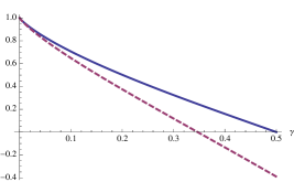
Figure 1: Amplitude damping channel with parameter $\gamma$: detected quantum capacity with maximally entangled input and estimation of $\vec{p}$ for the eigenstates of (33) and for the Bell basis (solid and dashed line, respectively).

We want to point out that the above scheme has been successfully tested experimentally for various models of qubit noise, including the phase damping, depolarising and amplitude damping channels described above, by using pairs of polarised photons qcdet-exp . We also want to stress that the detection method reviewed here can be applied also to multipartite quantum channels and it has proved to give a satisfactory theoretical performance in the case of two-qubit correlated channels in Ref. qcdet-corr .

We finally want to point out that all detectable bounds we are providing also give lower bounds to the private information $P$, since $P\geq Q_{1}$ NC00 . Moreover, we can also derive a detectable lower bound to the entanglement-assisted classical capacity. Actually, the latter is defined as CE

$$C_{E}=\max_{\rho}I(\rho,{\cal E}_{1})\;,$$ (36)

where $I(\rho,{\cal E}_{1})=S(\rho)+I_{c}(\rho,{\cal E}_{1})$. By considering the procedure outlined above we then have the lower bound

$$C_{E}\geq\log_{2}d+Q_{DET}\;,$$ (37)

where a maximally entangled state $|\Psi\rangle$ is considered as input, giving $S(\rho)=\log_{2}d$.

V Conclusions

In conclusion, we have reviewed in a unified way a method to detect properties based on convexity features of quantum channels, and more generally of quantum evolutions of open systems, and lower bounds to capacities of quantum communication channels, specifically to the quantum capacity, the entanglement assisted capacity, and the private capacity. The procedures we presented do not require any a priori knowledge about the quantum channel and rely on a number of measurement settings that scales as $d^{2}$. They are therefore much cheaper than full process tomography, whose number of measurements in the entanglement based scenario considered here scales as $d^{4}$. Moreover, they can be easily implementable in an experimental scenario without posing any particular restriction on the nature of the physical system under consideration. As shown in Sect. II, the method can be equivalently applied by suitably preparing the input and measuring the output system alone without necessarily requiring the use of entangled states. We also point out that the same scheme outlined in Sect. II can also be applied to detect non-Markovianity properties for some classes of dynamical maps in open quantum systems noma-wit .

References

- (1) I. L. Chuang and M. A. Nielsen, Journal of Modern Optics 44, 2455 (1997).
- (2) J. F. Poyatos, J. I. Cirac, and P. Zoller, Phys. Rev. Lett. 78, 390 (1997).
- (3) M. F. Sacchi, Phys. Rev. A 63, 054104 (2001).
- (4) G. M. D’Ariano and P. Lo Presti, Phys. Rev. Lett. 86, 4195 (2001).
- (5) J. Altepeter, D. Branning, E. Jeffrey, T. Wei, P. Kwiat, R. Thew, J. OBrien, M. Nielsen, and A. White, Phys. Rev. Lett. 90, 193601 (2003).
- (6) J. L. O’Brien, G. J. Pryde, A. Gilchrist, D. F. V. James, N. K. Langford, T. C. Ralph, and A. G. White, Phys. Rev. Lett. 93, 080502 (2004).
- (7) S. H. Myrskog, J. K. Fox, M. W. Mitchell, and A. M. Steinberg, Phys. Rev. A 72, 013615 (2005).
- (8) M. Riebe, K. Kim, P. Schindler, T. Monz, P. O. Schmidt, T. K. Körber, W. Hänsel, H. Häffner, C. F. Roos, and R. Blatt, Phys. Rev. Lett. 97, 220407 (2006).
- (9) M. Mohseni, A. T. Rezakhani, and D. A. Lidar, Phys. Rev. A 77, 032322 (2008).
- (10) I. Bongioanni, L. Sansoni, F. Sciarrino, G. Vallone, and P. Mataloni, Phys. Rev. A 82, 042307 (2010).
- (11) Yoav Sagi, Ido Almog, and Nir Davidson, Phys. Rev. Lett. 105, 053201 (2010).
- (12) C. Macchiavello and M. Rossi, Phys. Rev. A 88, 042335 (2013).
- (13) C. Macchiavello and M. F. Sacchi, Phys. Rev. Lett. 116, 140501 (2016).
- (14) A. Jamiolkowski, Rep. Math. Phys. 3, 275 (1972).
- (15) M.-D. Choi, Linear Algebr. Appl. 10, 285 (1975).
- (16) G. M. D’Ariano, P. Perinotti, and M. F. Sacchi, J. Opt. B 6, S487 (2004).
- (17) M. Horodecki, P. Horodecki, and R. Horodecki, Phys. Lett. A 223, 1 (1996); B. M. Terhal, Phys. Lett. A 271, 319 (2000).
- (18) O. Gühne et al, Phys. Rev. A 66, 062305 (2002).
- (19) A. O. Pittenger and M.H. Rubin, Opt. Comm. 179, 447 (2000).
- (20) O. Gühne et al, J. Mod. Opt. 50, 1079 (2003).
- (21) C. Macchiavello and M. Rossi, J. Phys.-Conf. Series 470, 012005 (2013).
- (22) A. Orieux, L. Sansoni, M. Persechino, P. Mataloni, M. Rossi, and C. Macchiavello, Phys. Rev. Lett. 111, 220501 (2013).
- (23) I. Devetak, IEEE Trans. Inf. Theory 51, 44 (2003).
- (24) S. Lloyd, Phys. Rev. A 55, 1613 (1997).
- (25) H. Barnum, M. A. Nielsen, and B. Schumacher, Phys. Rev. A 57, 4153 (1998).
- (26) B. W. Schumacher and M. A. Nielsen, Phys. Rev. A 54, 2629 (1996).
- (27) B. W. Schumacher, Phys. Rev. A 54, 2614 (1996).
- (28) M. A. Nielsen and I. L. Chuang, Quantum Information and Communication (Cambridge, Cambridge University Press, 2000).
- (29) D. Di Vincenzo, P. W. Shor, and J. Smolin, Phys. Rev. A 57, 830 (1998).
- (30) G. Smith, J. A. Smolin, and A. Winter, IEEE Trans. Info. Theory 54 (9), 4208 (2008).
- (31) V. Giovannetti and R. Fazio, Phys. Rev. A 71, 032314 (2005).
- (32) A. Cuevas, M. Proietti, M. A. Ciampini, S. Duranti, P. Mataloni, M. F. Sacchi, and C. Macchiavello, Phys. Rev. Lett. 119, 100502 (2017).
- (33) C. Macchiavello and M. F. Sacchi, Phys. Rev. A 94, 052333 (2016).
- (34) C.H. Bennett, P. W. Shor, J. Smolin and A.V. Thapliyal, Phys. Rev. Lett. 83, 3081 (1999).
- (35) D. Chruscinski, C. Macchiavello, and S. Maniscalco, Phys. Rev. Lett. 118, 080404 (2017).