Path-Based Spectral Clustering: Guarantees, Robustness to Outliers, and Fast Algorithms

\nameAnna Little \emaillittl119@msu.edu
\addrDepartment of Computational Mathematics, Science, and Engineering
Michigan State University, East Lansing, MI 48824, USA \AND\nameMauro Maggioni \emailmauromaggionijhu@icloud.com
\addrDepartment of Applied Mathematics and Statistics, Department of Mathematics
Johns Hopkins University, Baltimore, MD 21218, USA \AND\nameJames M. Murphy \emailjm.murphy@tufts.edu
\addrDepartment of Mathematics
Tufts University, Medford, MA 02139, USA
Abstract

We consider the problem of clustering with the longest-leg path distance (LLPD) metric, which is informative for elongated and irregularly shaped clusters. We prove finite-sample guarantees on the performance of clustering with respect to this metric when random samples are drawn from multiple intrinsically low-dimensional clusters in high-dimensional space, in the presence of a large number of high-dimensional outliers. By combining these results with spectral clustering with respect to LLPD, we provide conditions under which the Laplacian eigengap statistic correctly determines the number of clusters for a large class of data sets, and prove guarantees on the labeling accuracy of the proposed algorithm. Our methods are quite general and provide performance guarantees for spectral clustering with any ultrametric. We also introduce an efficient, easy to implement approximation algorithm for the LLPD based on a multiscale analysis of adjacency graphs, which allows for the runtime of LLPD spectral clustering to be quasilinear in the number of data points.

Keywords: unsupervised learning, spectral clustering, manifold learning, fast algorithms, shortest path distance.

1 Introduction

Clustering is a fundamental unsupervised problem in machine learning, seeking to detect group structures in data without any references or labeled training data. Determining clusters can become harder as the dimension of the data increases: one of the manifestations of the curse of dimension is that points drawn from high-dimensional distributions are far from their nearest neighbors, which can make noise and outliers challenging to address (Hughes, 1968; Györfi et al., 2006; Bellman, 2015). However, many clustering problems for real data involve data that exhibit low dimensional structure, which can be exploited to circumvent the curse of dimensionality. Various assumptions are imposed on the data to model low-dimensional structure, including requiring that the clusters be drawn from affine subspaces (Parsons et al., 2004; Chen and Lerman, 2009a, b; Vidal, 2011; Zhang et al., 2012; Elhamifar and Vidal, 2013; Wang et al., 2014; Soltanolkotabi et al., 2014) or more generally from low-dimensional mixture models (McLachlan and Basford, 1988; Arias-Castro, 2011; Arias-Castro et al., 2011, 2017).

When the shape of clusters is unknown or deviates from both linear structures (Vidal, 2011; Soltanolkotabi and Candes, 2012) or well-separated approximately spherical structures (for which K𝐾K-means performs well (Mixon et al., 2017)), spectral clustering (Ng et al., 2002; Von Luxburg, 2007) is a very popular approach, often robust with respect to the geometry of the clusters and of noise and outliers (Arias-Castro, 2011; Arias-Castro et al., 2011). Spectral clustering requires an initial distance or similarity measure, as it operates on a graph constructed between near neighbors measured and weighted based on such distance. In this article, we propose to analyze low-dimensional clusters when spectral clustering is based on the longest-leg path distance (LLPD) metric, in which the distance between points x,y𝑥𝑦x,y is the minimum over all paths between x,y𝑥𝑦x,y of the longest edge in the path. Distances in this metric exhibit stark phase transitions between within-cluster distances and between-cluster distances. We are interested in performance guarantees with this metric which will explain this phase transition. We prove theoretical guarantees on the performance of LLPD as a discriminatory metric, under the assumption that data is drawn randomly from distributions supported near low-dimensional sets, together with a possibly very large number of outliers sampled from a distribution in the high dimensional ambient space. Moreover, we show that LLPD spectral clustering correctly determines the number of clusters and achieves high classification accuracy for data drawn from certain non-parametric mixture models. The existing state-of-the-art for spectral clustering struggles in the highly noisy setting, in the case when clusters are highly elongated—which leads to large within-cluster variance for traditional distance metrics—and also in the case when clusters have disparate volumes. In contrast, our method can tolerate a large amount of noise, even in its natural non-parametric setting, and it is essentially invariant to geometry of the clusters.

In order to efficiently analyze large datasets, a fast algorithm for computing LLPD is required. Fast nearest neighbor searches have been developed for Euclidean distance on intrinsically low-dimensional sets (and other doubling spaces) using cover trees (Beygelzimer et al., 2006), among other popular algorithms (e.g. k𝑘k-d trees (Bentley, 1975)), and have been successfully employed in fast clustering algorithms. These algorithms compute the O(1)𝑂1O(1) nearest neighbors for all points in O(nlog(n))𝑂𝑛𝑛O(n\log(n)), where n𝑛n is the number of points, and are hence crucial to the scalability of many machine learning algorithms. LLPD seems to require the computation of a minimizer over a large set of paths. We introduce here an algorithm for LLPD, efficient and easy to implement, with the same quasilinear computational complexity as the algorithms above: this makes LLPD nearest neighbor searches scalable to large data sets. We moreover present a fast eigensolver for the (dense) LLPD graph Laplacian that allows for the computation of the approximate eigenvectors of this operator in essentially linear time.

1.1 Summary of Results

The major contributions of the present work are threefold.

First, we analyze the finite sample behavior of LLPD for points drawn according to a flexible probabilistic data model, with points drawn from low dimensional structures contaminated by a large number of high dimensional outliers. We derive bounds for maximal within-cluster LLPD and minimal between-cluster LLPD that hold with high probability, and also derive a lower bound for the minimal LLPD to a point’s knsesubscript𝑘nse{k_{\text{nse}}} nearest neighbor in the LLPD metric. These results rely on a combination of techniques from manifold learning and percolation theory, and may be of independent interest.

Second, we deploy these finite sample results to prove that, under our data model, the eigengap statistic for LLPD-based Laplacians correctly determines the number of clusters. While the eigengap heuristic is often used in practice, existing theoretical analyses of spectral clustering fail to provide a rich class of data for which this estimate is provably accurate. Our results regarding the eigengap are quite general and can be applied to give state-of-the-art performance guarantees for spectral clustering with any ultrametric, not just the LLPD. Moreover, we prove that the LLPD-based spectral embedding learned by our method is clustered correctly by K𝐾K-means with high probability, with misclassification rate improving over the existing state-of-the-art for Euclidean spectral clustering.

Finally, we present a fast and easy to implement approximation algorithm for LLPD, based on a multiscale decomposition of adjacency graphs. Let ksubscript𝑘{k_{\ell\ell}} be the number of LLPD nearest neighbors sought. Our approach generates approximate ksubscript𝑘{k_{\ell\ell}}-nearest neighbors in the LLPD at a cost of O(n(kEucCNN+m(kEuclog(n))+k)),𝑂𝑛subscript𝑘Eucsubscript𝐶NN𝑚subscript𝑘Euc𝑛subscript𝑘O(n({k_{\text{Euc}}}C_{\text{NN}}+m({k_{\text{Euc}}}\vee\log(n))+{k_{\ell\ell}})), where n𝑛n is the number of data points, kEucsubscript𝑘Euc{k_{\text{Euc}}} is the number of nearest neighbors used to construct an initial adjacency graph on the data, CNNsubscript𝐶NNC_{\text{NN}} is the cost of a Euclidean nearest neighbor query, m𝑚m is related to the approximation scheme, and \vee denotes the maximum. Under the realistic assumption kEuc,k,mlog(n)much-less-thansubscript𝑘Eucsubscript𝑘𝑚𝑛{k_{\text{Euc}}},{k_{\ell\ell}},m\ll\log(n), this algorithm is O(nlog2(n))𝑂𝑛superscript2𝑛O(n\log^{2}(n)) for data with low intrinsic dimension. If kEuc,k,m=O(1)subscript𝑘Eucsubscript𝑘𝑚𝑂1{k_{\text{Euc}}},{k_{\ell\ell}},m=O(1) with respect to n𝑛n, this reduces to O(nlog(n))𝑂𝑛𝑛O(n\log(n)). We quantify the resulting approximation error, which can be uniformly bounded independent of the data. We moreover develop a fast eigensolver to compute the K𝐾K principal eigenfunctions of the dense approximate LLPD Laplacian in O(n(kEucCNN+m(kEuclog(n)K2)))𝑂𝑛subscript𝑘Eucsubscript𝐶NN𝑚subscript𝑘Euc𝑛superscript𝐾2O(n({k_{\text{Euc}}}C_{\text{NN}}+m({k_{\text{Euc}}}\vee\log(n)\vee K^{2}))) time. If kEuc,K,m=O(1)subscript𝑘Euc𝐾𝑚𝑂1{k_{\text{Euc}}},K,m=O(1) with respect to n𝑛n, this reduces to O(nlog(n))𝑂𝑛𝑛O(n\log(n)). This allows for the fast computation of the eigenvectors without resorting to constructing a sparse Laplacian. The proposed method is demonstrated on a variety of synthetic and real datasets, with performance consistently with our theoretical results.

Article outline. In Section 2, we present an overview of clustering methods, with an emphasis on those most closely related to the one we propose. A summary of our data model and main results, together with motivating examples, are in Section 3. In Section 4, we analyze the LLPD for non-parametric mixture models. In Section 5, performance guarantees for spectral clustering with LLPD are derived, including guarantees on when the eigengap is informative and on the accuracy of clustering the spectral embedding obtained from the LLPD graph Laplacian. Section 6 proposes an efficient approximation algorithm for LLPD yielding faster nearest neighbor searches and computation of the eigenvectors of the LLPD Laplacian. Numerical experiments on representative datasets appear in Section 7. We conclude and discuss new research directions in Section 8.

1.2 Notation

In Table 1, we introduce notation we will use throughout the article.

X={xi}i=1nD𝑋superscriptsubscriptsubscript𝑥𝑖𝑖1𝑛superscript𝐷X=\{x_{i}\}_{i=1}^{n}\subset\mathbb{R}^{D} Data points to cluster
d𝑑d Intrinsic dimension of cluster sets
K𝐾K Number of clusters
{Xl}l=1Ksuperscriptsubscriptsubscript𝑋𝑙𝑙1𝐾\{X_{l}\}_{l=1}^{K} Discrete data clusters
X~~𝑋\tilde{X} Discrete noise data
XNsubscript𝑋𝑁X_{N} Denoised data; XNXsubscript𝑋𝑁𝑋X_{N}\subseteq X
N𝑁N Number of points remaining after denoising
nminsubscript𝑛minn_{\text{min}} Smallest number of points in a cluster
kEucsubscript𝑘Euc{k_{\text{Euc}}} Number of nearest neighbors in construction of initial NN-graph
ksubscript𝑘{k_{\ell\ell}} Number of nearest neighbors for LLPD
knsesubscript𝑘nse{k_{\text{nse}}} Number of nearest neighbors for LLPD denoising
CNNsubscript𝐶NNC_{\text{NN}} Complexity of computing a Euclidean NN
W𝑊W Weight matrix
LSYMsubscript𝐿SYM{L_{\text{SYM}}} Symmetric normalized Laplacian
σ𝜎\sigma Scaling parameter in construction of weight matrix
{(ϕi,λi)}i=1nsuperscriptsubscriptsubscriptitalic-ϕ𝑖subscript𝜆𝑖𝑖1𝑛\{(\phi_{i},\lambda_{i})\}_{i=1}^{n} Eigenvectors and eigenvalues of an n×n𝑛𝑛n\times n LSYMsubscript𝐿SYM{L_{\text{SYM}}}
ϵinsubscriptitalic-ϵin\epsilon_{\mathrm{in}} Maximum within cluster LLPD; see (3.2)
ϵnsesubscriptitalic-ϵnse\epsilon_{\mathrm{nse}} Minimum LLPD of noise points to knsesubscript𝑘nse{k_{\text{nse}}} nearest neighbor; see (3.2)
ϵbtwsubscriptitalic-ϵbtw\epsilon_{\mathrm{btw}} Minimum between cluster LLPD; see (3.2)
ϵsepsubscriptitalic-ϵsep\epsilon_{\mathrm{sep}} Minimum between cluster LLPD after denoising; see (5.3)
δ𝛿\delta Minimum Euclidean distance between clusters; see Definition 3.2
θ𝜃\theta Denoising parameter; see Definition 3.6
ζn,ζθsubscript𝜁𝑛subscript𝜁𝜃\zeta_{n},\zeta_{\theta} LDLN data cluster balance parameters; see (3.1)
ζNsubscript𝜁𝑁\zeta_{N} Empirical cluster balance parameter after denoising; see Assumption 1
ρ𝜌\rho Arbitrary metric
ρsubscript𝜌\rho_{\ell\ell} LLPD metric; see Definition 2.1
dsuperscript𝑑\mathcal{H}^{d} d𝑑d-dimensional Hausdorff measure
Bϵ(x)subscript𝐵italic-ϵ𝑥B_{\epsilon}(x) D𝐷D-dimensional ball of radius ϵitalic-ϵ\epsilon centered at x𝑥x
B1subscript𝐵1B_{1} Unit ball, with dimension clear from context
ab𝑎𝑏a\vee b, ab𝑎𝑏a\wedge b Maximum, minimum of a𝑎a and b𝑏b
abless-than-or-similar-to𝑎𝑏a\lesssim b, abgreater-than-or-equivalent-to𝑎𝑏a\gtrsim b aCb𝑎𝐶𝑏a\leq Cb , aCb𝑎𝐶𝑏a\geq Cb for some absolute constant C>0𝐶0C>0
Table 1: Notation used throughout the article.

2 Background

2.1 Background on Clustering

The process of determining groupings within data and assigning labels to data points according to these groupings without supervision is called clustering (Hastie et al., 2009). It is a fundamental problem in machine learning, with many approaches known to perform well in certain circumstances, but not in others. In order to provide performance guarantees, analytic, geometric, or statistical assumptions are placed on the data. Perhaps the most popular clustering scheme is K𝐾K-means (Steinhaus, 1957; Friedman et al., 2001; Hastie et al., 2009), together with its variants (Ostrovsky et al., 2006; Arthur and Vassilvitskii, 2007; Park and Jun, 2009), which are used in conjunction with feature extraction methods. This approach partitions the data into a user-specified number K𝐾K groups, where the partition is chosen to minimize within-cluster dissimilarity: C=argminC={Ck}k=1Kk=1KxCkxx¯k22.superscript𝐶subscriptargmin𝐶superscriptsubscriptsubscript𝐶𝑘𝑘1𝐾superscriptsubscript𝑘1𝐾subscript𝑥subscript𝐶𝑘superscriptsubscriptnorm𝑥subscript¯𝑥𝑘22C^{*}=\operatorname*{arg\,min}_{C=\{C_{k}\}_{k=1}^{K}}\sum_{k=1}^{K}\sum_{x\in C_{k}}\|x-\bar{x}_{k}\|_{2}^{2}. Here, {Ck}k=1Ksuperscriptsubscriptsubscript𝐶𝑘𝑘1𝐾\{C_{k}\}_{k=1}^{K} is a partition of the points, Cksubscript𝐶𝑘C_{k} is the set of points in the kthsuperscript𝑘𝑡k^{th} cluster and x¯ksubscript¯𝑥𝑘\bar{x}_{k} denotes the mean of the kthsuperscript𝑘𝑡k^{th} cluster. Unfortunately, the K𝐾K-means algorithm and its refinements perform poorly for datasets that are not the union of well-separated, spherical clusters, and are very sensitive to outliers. In general, density-based methods such as density-based spatial clustering of applications with noise (DBSCAN) and variants (Ester et al., 1996; Xu et al., 1998) or spectral methods (Shi and Malik, 2000; Ng et al., 2002) are required to handle irregularly shaped clusters.

2.2 Hierarchical Clustering

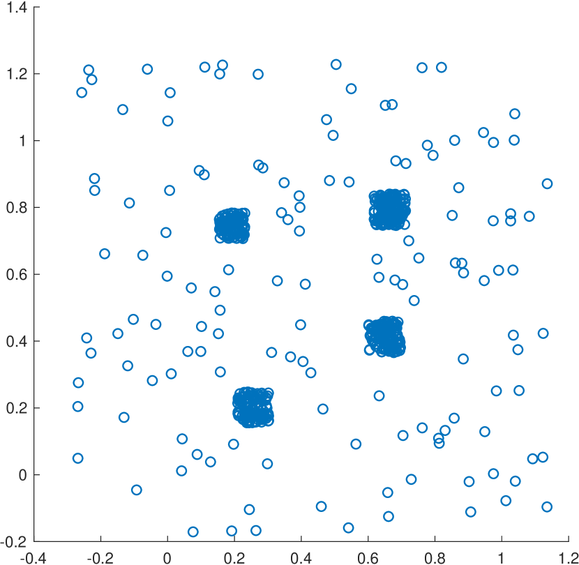
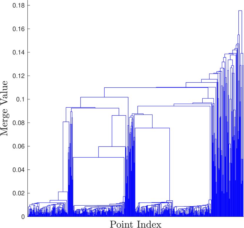
Hierarchical clustering algorithms build a family of clusters at distinct hierarchical levels. Their results are readily presented as a dendrogram (see Figure 1). Hierarchical clustering algorithms can be agglomerative, where individual points start as their own clusters and are iteratively merged, or divisive, where the full dataset is iteratively split until some stopping criterion is reached. It is often challenging to infer a global partition of the data from hierarchical algorithms, as it is unclear where to cut the dendrogram.
Refer to caption
(a) Data to cluster
Refer to caption
(b) Corresponding single linkage dendrogram
Figure 1: Four two-dimensional clusters together with noise (Zelnik-Manor and Perona, 2004) appear in (a). In (b) is the corresponding single-linkage dendrogram. Each point begins as its own cluster, and at each level of the dendrogram, the two nearest clusters are merged. It is hard to distinguish between the noise and cluster points from the single linkage dendrogram, as it is not obvious where the four clusters are.

For agglomerative methods, it must be determined which clusters ought to be merged at a given iteration. This is done by a cluster dissimilarity metric ρcsubscript𝜌𝑐\rho_{c}. For two clusters Ci,Cjsubscript𝐶𝑖subscript𝐶𝑗C_{i},C_{j}, ρc(Ci,Cj)subscript𝜌𝑐subscript𝐶𝑖subscript𝐶𝑗\rho_{c}(C_{i},C_{j}) small means the clusters are candidates for merger. Let ρXsubscript𝜌𝑋\rho_{X} be a metric defined on all the data points in X𝑋X. Standard ρcsubscript𝜌𝑐\rho_{c}, and the corresponding clustering methods, include:

  • \cdot

    ρSL(Ci,Cj)=minxiCi,xjCjρX(xi,xj)subscript𝜌𝑆𝐿subscript𝐶𝑖subscript𝐶𝑗subscriptformulae-sequencesubscript𝑥𝑖subscript𝐶𝑖subscript𝑥𝑗subscript𝐶𝑗subscript𝜌𝑋subscript𝑥𝑖subscript𝑥𝑗\rho_{SL}(C_{i},C_{j})=\min_{x_{i}\in C_{i},x_{j}\in C_{j}}\rho_{X}(x_{i},x_{j}): single linkage clustering.

  • \cdot

    ρCL(Ci,Cj)=maxxiCi,xjCjρX(xi,xj)subscript𝜌𝐶𝐿subscript𝐶𝑖subscript𝐶𝑗subscriptformulae-sequencesubscript𝑥𝑖subscript𝐶𝑖subscript𝑥𝑗subscript𝐶𝑗subscript𝜌𝑋subscript𝑥𝑖subscript𝑥𝑗\rho_{CL}(C_{i},C_{j})=\max_{x_{i}\in C_{i},x_{j}\in C_{j}}\rho_{X}(x_{i},x_{j}): complete linkage clustering.

  • \cdot

    ρGA(Ci,Cj)=1|CiCj|xiCixjCjρX(xi,xj)\rho_{GA}(C_{i},C_{j})=\frac{1}{|C_{i}\|C_{j}|}\sum_{x_{i}\in C_{i}}\sum_{x_{j}\in C_{j}}\rho_{X}(x_{i},x_{j}): group average clustering.

In Section 6 we make theoretical and practical connections between the proposed method and single linkage clustering.

2.3 Spectral Clustering

Spectral clustering methods (Shi and Malik, 2000; Meila and Shi, 2001; Ng et al., 2002; Von Luxburg, 2007) use a spectral decomposition of an adjacency or Laplacian matrix to define an embedding of the data, and then cluster the embedded data using a standard algorithm, commonly K𝐾K-means. The basic idea is to construct a weighted graph on the data that represents local relationships. The graph has low edge weights for points far apart from each other and high edge weights for points close together. This graph is then partitioned into clusters so that there are large edge weights within each cluster, and small edge weights between each cluster. Spectral clustering in fact relaxes an NP-hard graph partition problem (Chung, 1997; Shi and Malik, 2000).

We now introduce notation related to spectral clustering that will be used throughout this work. Let fσ:[0,1]:subscript𝑓𝜎01f_{\sigma}:\mathbb{R}\rightarrow[0,1] denote a kernel function with scale parameter σ𝜎\sigma. Given a metric ρ:D×D[0,):𝜌superscript𝐷superscript𝐷0\rho:\mathbb{R}^{D}\times\mathbb{R}^{D}\rightarrow[0,\infty) and some discrete set X={xi}i=1nD𝑋superscriptsubscriptsubscript𝑥𝑖𝑖1𝑛superscript𝐷X=\{x_{i}\}_{i=1}^{n}\subset\mathbb{R}^{D}, let Wij=fσ(ρ(xi,xj))subscript𝑊𝑖𝑗subscript𝑓𝜎𝜌subscript𝑥𝑖subscript𝑥𝑗W_{ij}=f_{\sigma}(\rho(x_{i},x_{j})) be the corresponding weight matrix. Let di=j=1nWijsubscript𝑑𝑖superscriptsubscript𝑗1𝑛subscript𝑊𝑖𝑗d_{i}=\sum_{j=1}^{n}W_{ij} denote the degree of point xisubscript𝑥𝑖x_{i}, and define the diagonal degree matrix Dii=di,Dij=0formulae-sequencesubscript𝐷𝑖𝑖subscript𝑑𝑖subscript𝐷𝑖𝑗0{D}_{ii}=d_{i},{D}_{ij}=0 for ij𝑖𝑗i\neq j. The graph Laplacian is then defined by L=DW,𝐿𝐷𝑊L={D}-W, which is often normalized to obtain the symmetric Laplacian LSYM=ID12WD12subscript𝐿SYM𝐼superscript𝐷12𝑊superscript𝐷12{L_{\text{SYM}}}=I-{D}^{-\frac{1}{2}}W{D}^{-\frac{1}{2}} or random walk Laplacian LRW=ID1W.subscript𝐿RW𝐼superscript𝐷1𝑊L_{\text{RW}}=I-{D}^{-1}W. Using the eigenvectors of L𝐿L to define an embedding leads to unnormalized spectral clustering, whereas using the eigenvectors of LSYMsubscript𝐿SYM{L_{\text{SYM}}} or LRWsubscript𝐿RWL_{\text{RW}} leads to normalized spectral clustering. While both normalized and unnormalized spectral clustering minimize between-cluster similarity, only normalized spectral clustering maximizes within-cluster similarity, and is thus preferred in practice (Von Luxburg, 2007).

In this article we consider spectral clustering with LSYMsubscript𝐿SYM{L_{\text{SYM}}} and construct the spectral embedding defined according to the popular algorithm of Ng et al. (2002). When appropriate, we will use LSYM(X,ρ,fσ)subscript𝐿SYM𝑋𝜌subscript𝑓𝜎{L_{\text{SYM}}}(X,\rho,f_{\sigma}) to denote the matrix LSYMsubscript𝐿SYM{L_{\text{SYM}}} computed on the data set X𝑋X using metric ρ𝜌\rho and kernel fσsubscript𝑓𝜎f_{\sigma}. We denote the eigenvalues of LSYMsubscript𝐿SYM{L_{\text{SYM}}} (which are identical to those of LRWsubscript𝐿RWL_{\text{RW}}) by λ1λnsubscript𝜆1subscript𝜆𝑛\lambda_{1}\leq\ldots\leq\lambda_{n}, and the corresponding eigenvectors by ϕ1,,ϕnsubscriptitalic-ϕ1subscriptitalic-ϕ𝑛\phi_{1},\ldots,\phi_{n}. To cluster the data into K𝐾K groups according to Ng et al. (2002), one first forms an n×K𝑛𝐾n\times K matrix ΦΦ\Phi whose columns are given by {ϕi}i=1Ksuperscriptsubscriptsubscriptitalic-ϕ𝑖𝑖1𝐾\{\phi_{i}\}_{i=1}^{K}; these K𝐾K eigenvectors are called the K𝐾K principal eigenvectors. The rows of ΦΦ\Phi are then normalized to obtain the matrix V𝑉V, that is Vij=Φij/(jΦij2)1/2subscript𝑉𝑖𝑗subscriptΦ𝑖𝑗superscriptsubscript𝑗subscriptsuperscriptΦ2𝑖𝑗12V_{ij}={\Phi_{ij}}/({{\sum_{j}\Phi^{2}_{ij}}})^{1/2}. Let {𝐯i}i=1nKsuperscriptsubscriptsubscript𝐯𝑖𝑖1𝑛superscript𝐾\{\mathbf{v}_{i}\}_{i=1}^{n}\in\mathbb{R}^{K} denote the rows of V𝑉V. Note that if we let g:DK:𝑔superscript𝐷superscript𝐾g:\mathbb{R}^{D}\rightarrow\mathbb{R}^{K} denote the spectral embedding, 𝐯i=g(xi)subscript𝐯𝑖𝑔subscript𝑥𝑖\mathbf{v}_{i}=g(x_{i}). Finally, K𝐾K-means is applied to cluster the {𝐯i}i=1nsuperscriptsubscriptsubscript𝐯𝑖𝑖1𝑛\{\mathbf{v}_{i}\}_{i=1}^{n} into K𝐾K groups, which defines a partition of our data points {xi}i=1nsuperscriptsubscriptsubscript𝑥𝑖𝑖1𝑛\{x_{i}\}_{i=1}^{n}. One can use LRWsubscript𝐿RWL_{\text{RW}} similarly (Shi and Malik, 2000).

Choosing K𝐾K is an important aspect of spectral clustering, and various spectral-based mechanisms have been proposed in the literature (Azran and Ghahramani, 2006b, a; Zelnik-Manor and Perona, 2004; Sanguinetti et al., 2005). The eigenvalues of LSYMsubscript𝐿SYM{L_{\text{SYM}}} have often been used to heuristically estimate the number of clusters as the largest empirical eigengap K^=argmaxiλi+1λi,^𝐾subscriptargmax𝑖subscript𝜆𝑖1subscript𝜆𝑖\hat{K}=\operatorname*{arg\,max}_{i}\lambda_{i+1}-\lambda_{i}, although there are many data sets for which this heuristic is known to fail (Von Luxburg, 2007); this estimate is called the eigengap statistic. We remark that sometimes in the literature it is required that not only should λK^+1λK^subscript𝜆^𝐾1subscript𝜆^𝐾\lambda_{\hat{K}+1}-\lambda_{\hat{K}} be maximal, but also that λisubscript𝜆𝑖\lambda_{i} should be close to 0 for iK^𝑖^𝐾i\leq\hat{K}; we shall not make this additional assumption on λi,iK^subscript𝜆𝑖𝑖^𝐾\lambda_{i},i\leq\hat{K}, though we find in practice it is usually satisfied when the eigengap is accurate.

A description of the spectral clustering algorithm of Ng et al. (2002) in the case that K𝐾K is not known a priori appears in Algorithm 1; the algorithm can be modified in the obvious way if K𝐾K is known and does not need to be estimated, or when using a sparse Laplacian, for example when W𝑊W is defined by a sparse nearest neighbors graph.

Algorithm 1 Spectral Clustering with metric ρ𝜌\rho

Input: {xi}i=1nsuperscriptsubscriptsubscript𝑥𝑖𝑖1𝑛\{x_{i}\}_{i=1}^{n} (Data) , σ>0𝜎0\sigma>0 (Scaling parameter)
Output: Y𝑌Y (Labels)

1:  Compute the weight matrix Wn×n𝑊superscript𝑛𝑛W\in\mathbb{R}^{n\times n} with Wij=exp(ρ(xi,xj)2/σ2)subscript𝑊𝑖𝑗𝜌superscriptsubscript𝑥𝑖subscript𝑥𝑗2superscript𝜎2W_{ij}=\exp(-\rho(x_{i},x_{j})^{2}/\sigma^{2}).
2:  Compute the diagonal degree matrix Dn×n𝐷superscript𝑛𝑛D\in\mathbb{R}^{n\times n} with Dii=j=1nWijsubscript𝐷𝑖𝑖superscriptsubscript𝑗1𝑛subscript𝑊𝑖𝑗D_{ii}=\sum_{j=1}^{n}W_{ij}.
3:  Form the symmetric normalized Laplacian LSYM=ID12WD12subscript𝐿SYM𝐼superscript𝐷12𝑊superscript𝐷12{L_{\text{SYM}}}=I-D^{-\frac{1}{2}}WD^{-\frac{1}{2}}.
4:  Compute the eigendecomposition {(ϕk,λk)}k=1nsuperscriptsubscriptsubscriptitalic-ϕ𝑘subscript𝜆𝑘𝑘1𝑛\{(\phi_{k},\lambda_{k})\}_{k=1}^{n}, sorted so that 0=λ1λ2λn0subscript𝜆1subscript𝜆2subscript𝜆𝑛0=\lambda_{1}\leq\lambda_{2}\leq\dots\leq\lambda_{n}.
5:  Estimate the number of clusters K𝐾K as K^=argmaxkλk+1λk^𝐾subscriptargmax𝑘subscript𝜆𝑘1subscript𝜆𝑘\hat{K}=\operatorname*{arg\,max}_{k}\lambda_{k+1}-\lambda_{k}.
6:  For 1in1𝑖𝑛1\leq i\leq n, let 𝐯i=(ϕ1(xi),ϕ2(xi),,ϕK^(xi))/(ϕ1(xi),ϕ2(xi),,ϕK^(xi))2subscript𝐯𝑖subscriptitalic-ϕ1subscript𝑥𝑖subscriptitalic-ϕ2subscript𝑥𝑖subscriptitalic-ϕ^𝐾subscript𝑥𝑖subscriptnormsubscriptitalic-ϕ1subscript𝑥𝑖subscriptitalic-ϕ2subscript𝑥𝑖subscriptitalic-ϕ^𝐾subscript𝑥𝑖2\mathbf{v}_{i}=(\phi_{1}(x_{i}),\phi_{2}(x_{i}),\dots,\phi_{\hat{K}}(x_{i}))/||(\phi_{1}(x_{i}),\phi_{2}(x_{i}),\dots,\phi_{\hat{K}}(x_{i}))||_{2} define the (row normalized) spectral embedding.
7:  Compute labels Y𝑌Y by running K𝐾K-means on the data {𝐯i}i=1nsuperscriptsubscriptsubscript𝐯𝑖𝑖1𝑛\{\mathbf{v}_{i}\}_{i=1}^{n} using K^^𝐾\hat{K} as the number of clusters.

In addition to determining K𝐾K, performance guarantees for K𝐾K-means (or other clustering methods) on the spectral embedding is a topic of active research (Schiebinger et al., 2015; Arias-Castro et al., 2017). However, spectral clustering typically has poor performance in the presence of noise and highly elongated clusters.

2.4 Background on LLPD

Many clustering and machine learning algorithms make use of Euclidean distances to compare points. While universal and popular, this distance is data-independent, not adapted to the geometry of the data. Many data-dependent metrics have been developed, for example diffusion distances (Coifman et al., 2005; Coifman and Lafon, 2006), which are induced by diffusion processes on a dataset, and path-based distances (Fischer and Buhmann, 2003; Chang and Yeung, 2008). We shall consider a path-based distance for undirected graphs.

Definition 2.1

For X={xi}i=1nD𝑋superscriptsubscriptsubscript𝑥𝑖𝑖1𝑛superscript𝐷X=\{x_{i}\}_{i=1}^{n}\subset\mathbb{R}^{D}, let G𝐺G be the complete graph on X𝑋X with edges weighted by Euclidean distance between points. For xi,xjXsubscript𝑥𝑖subscript𝑥𝑗𝑋x_{i},x_{j}\in X, let 𝒫(xi,xj)𝒫subscript𝑥𝑖subscript𝑥𝑗\mathcal{P}(x_{i},x_{j}) denote the set of all paths connecting xi,xjsubscript𝑥𝑖subscript𝑥𝑗x_{i},x_{j} in G𝐺G. The longest-leg path distance (LLPD) is:

ρ(xi,xj)=min{yl}l=1L𝒫(xi,xj)maxl=1,2,,L1yl+1yl2.subscript𝜌subscript𝑥𝑖subscript𝑥𝑗subscriptsuperscriptsubscriptsubscript𝑦𝑙𝑙1𝐿𝒫subscript𝑥𝑖subscript𝑥𝑗subscript𝑙12𝐿1subscriptnormsubscript𝑦𝑙1subscript𝑦𝑙2\displaystyle\rho_{\ell\ell}(x_{i},x_{j})=\min_{\{y_{l}\}_{l=1}^{L}\in\mathcal{P}(x_{i},x_{j})}\max_{l=1,2,\dots,L-1}\|y_{l+1}-y_{l}\|_{2}.

In this article we use LLPD with respect to the Euclidean distance, but our results very easily generalize to other base distances. Our goal is to analyze the effects of transforming an original metric through the min-max distance along paths in the definition of LLPD above. We note that the LLPD is an ultrametric, i.e.

x,y,zXρ(x,y)max{ρ(x,z),ρ(y,z)}.formulae-sequencefor-all𝑥𝑦𝑧𝑋subscript𝜌𝑥𝑦subscript𝜌𝑥𝑧subscript𝜌𝑦𝑧\displaystyle\forall x,y,z\in X\quad\rho_{\ell\ell}(x,y)\leq\max\{\rho_{\ell\ell}(x,z),\rho_{\ell\ell}(y,z)\}\,. (2.1)

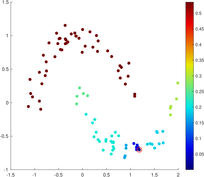
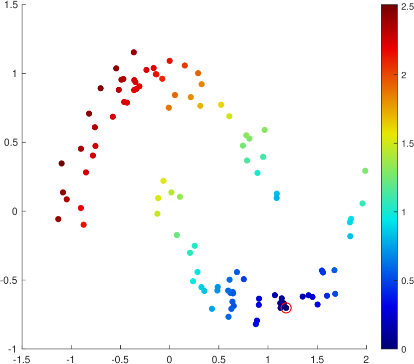
This property is central to the proofs of Sections 4 and 5. Figure 2 illustrates how LLPD successfully differentiates elongated clusters, whereas Euclidean distance does not.
Refer to caption
(a) LLPD from the marked point.
Refer to caption
(b) Euclidean distances from the marked point.
Figure 2: In this example, LLPD is compared with Euclidean distance. The distance from the red circled source point is shown in each subfigure. Notice that the LLPD has a phase transition that separates the clusters clearly, and that all distances within-cluster are comparable.

2.4.1 Probabilistic Analysis of LLPD

Existing theoretical analysis of LLPD is based on studying the uniform distribution on certain geometric sets. The degree and connectivity properties of near-neighbor graphs defined on points sampled uniformly from [0,1]dsuperscript01𝑑[0,1]^{d} and their connections with percolation have been studied extensively (Appel and Russo, 1997a, b, 2002; Penrose, 1997, 1999). Related results in the case of points drawn from low-dimensional structures were studied by Arias-Castro (2011). These results motivate some of the ideas in this article; detailed references are given below when appropriate.

2.4.2 Spectral Clustering with LLPD

Spectral clustering with LLPD has been shown to enjoy good empirical performance (Fischer et al., 2001; Fischer and Buhmann, 2003; Fischer et al., 2004) and is made more robust by incorporating outlier removal (Chang and Yeung, 2008). The method and its variants generally perform well for non-convex and highly elongated clusters, even in the presence of noise. However, no theoretical guarantees seem to be available. Moreover, numerical implementation of LLPD spectral clustering appears underdeveloped, and existing methods have been evaluated mainly on small, low-dimensional datasets. This article derives theoretical guarantees on performance of LLPD spectral clustering which confirms empirical insights, and also provides a fast implementation of the method suitable for large datasets.

2.4.3 Computing LLPD

The problem of computing this distance is referred to by many names in the literature, including the maximum capacity path problem, the widest path problem, and the bottleneck edge query problem (Pollack, 1960; Hu, 1961; Camerini, 1978; Gabow and Tarjan, 1988). A naive computation of LLPD distances is expensive, since the search space 𝒫(x,y)𝒫𝑥𝑦\mathcal{P}(x,y) is potentially very large. However, for a fixed pair of points x,y𝑥𝑦x,y connected in a graph G=G(V,E)𝐺𝐺𝑉𝐸G=G(V,E), ρ(x,y)subscript𝜌𝑥𝑦\rho_{\ell\ell}(x,y) can be computed in O(|E|)𝑂𝐸O(|E|) (Punnen, 1991). There has also been significant work on the related problem of finding bottleneck spanning trees. For a fixed root vertex sV𝑠𝑉s\in V, the minimal bottleneck spanning tree rooted at s𝑠s is the spanning tree whose maximal edge length is minimal. The bottleneck spanning tree can be computed in O(min{nlog(n)+|E|,|E|log(n)})𝑂𝑛𝑛𝐸𝐸𝑛O(\min\{n\log(n)+|E|,|E|\log(n)\}) (Camerini, 1978; Gabow and Tarjan, 1988).

Computing all LLPDs for all points is the all points path distance (APPD) problem. Naively applying the bottleneck spanning tree construction to each point gives an APPD runtime of O(min{n2log(n)+n|E|,n|E|log(n)})𝑂superscript𝑛2𝑛𝑛𝐸𝑛𝐸𝑛O(\min\{n^{2}\log(n)+n|E|,n|E|\log(n)\}). However the APPD distance matrix can be computed in O(n2)𝑂superscript𝑛2O(n^{2}), for example with a modified SLINK algorithm (Sibson, 1973), or with Cartesian trees (Alon and Schieber, 1987; Demaine et al., 2009, 2014). We propose to approximate LLPD and implement LLPD spectral clustering with an algorithm near-linear in n𝑛n, which enables the analysis of very large datasets (see Section 6).

3 Major Contributions

In this section we present a simplified version of our main theoretical result. More general versions of these results, with detailed constants, will follow in Sections 4 and 5. We first discuss a motivating example and outline our data model and assumptions, which will be referred to throughout the article.

3.1 Motivating Examples
Refer to caption
(a) Original dataset.
Refer to caption
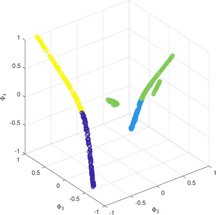
(b) 3 dimensional spectral embedding with Euclidean distances, labeled with K𝐾K-means. The data has been denoised based on thresholding with Euclidean distances.
Refer to caption
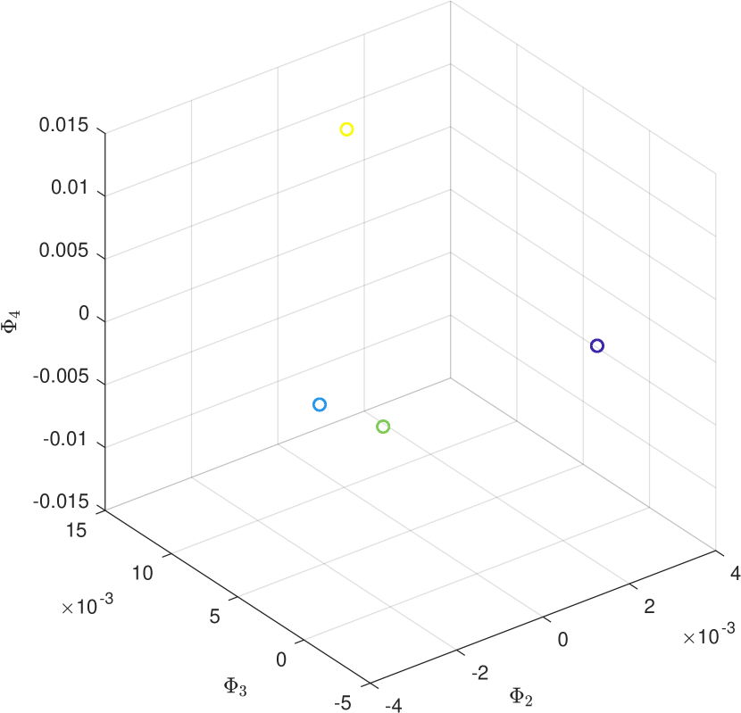
(c) 3 dimensional spectral embedding with LLPD, labeled with K𝐾K-means. The data has been denoised based on thresholding with LLPD.
Refer to caption
(d) K𝐾K-means labels.
Refer to caption
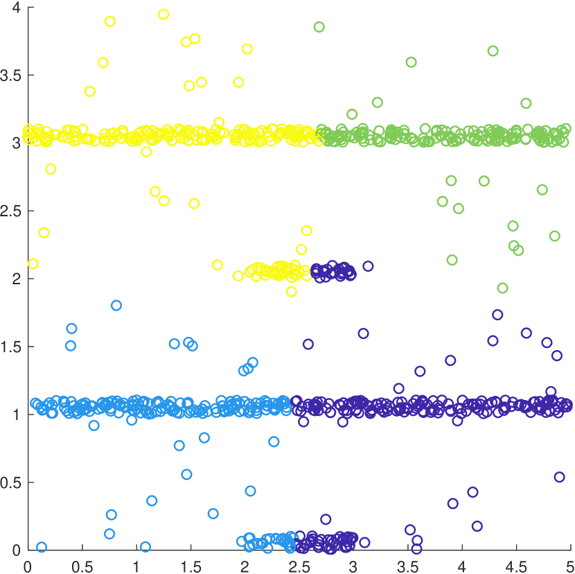
(e) Spectral clustering results with Euclidean distances.
Refer to caption
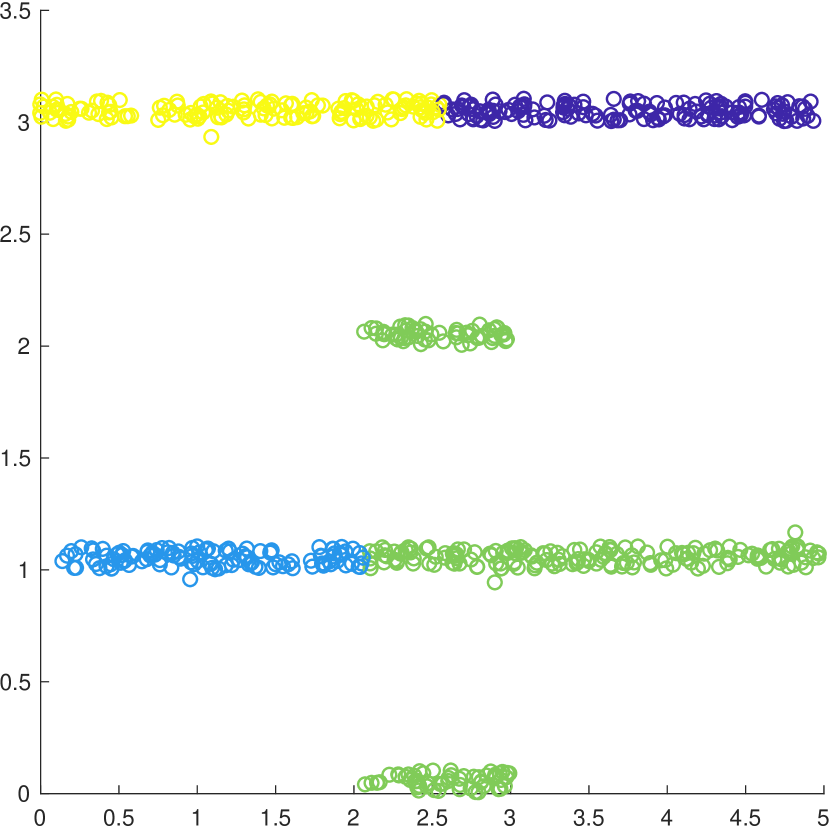
(f) Spectral clustering results with LLPD.
Figure 3: The dataset consists of four elongated clusters in 2superscript2\mathbb{R}^{2}, together with ambient noise. The labels given by K𝐾K-means are quite inaccurate, as are those given by regular spectral clustering. The labels given by LLPD spectral clustering are perfect. Note that ΦisubscriptΦ𝑖\Phi_{i} denotes the ithsuperscript𝑖𝑡i^{th} principal eigenvector of LSYMsubscript𝐿SYM{L_{\text{SYM}}}. For both variants of spectral clustering, the K𝐾K-means algorithm was run in the 4 dimensional embedding space given by the first 4 principal eigenvectors of LSYMsubscript𝐿SYM{L_{\text{SYM}}}.

In this subsection we illustrate in which regimes LLPD spectral clustering advances the state-of-art for clustering. As will be explicitly described in Subsection 3.2, we model clusters as connected, high-density regions, and we model noise as a low-density region separating the clusters. Our method easily handles highly elongated and irregularly shaped clusters, where traditional K𝐾K-means and even spectral clustering fail. For example, consider the four elongated clusters in 2superscript2\mathbb{R}^{2} illustrated in Figure 3. Both K𝐾K-means and Euclidean spectral clustering split one or more of the most elongated clusters, whereas the LLPD spectral embedding perfectly separates them. Moreover, the eigenvalues of the LLPD Laplacian correctly infer there are 4 clusters, unlike the Euclidean Laplacian.

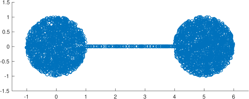
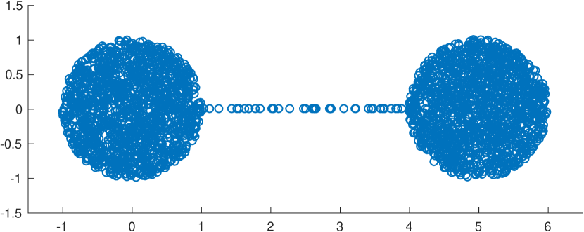
There are naturally situations where LLPD spectral clustering will not perform well, such as for certain types of structured noise. For example, consider the dumbbell shown in Figure 4. When there is a high-density bridge connecting the dumbbell, LLPD will not be able to distinguish the two balls. However, it is worth noting that this property is precisely what allows for robust performance with elongated clusters, and that if the bridge has a lower density than the clusters, LLPD spectral clustering performs very well.
Refer to caption
(a) Two clusters connected by a bridge of roughly the same empirical density.
Refer to caption
(b) Two clusters connected by a bridge of lower empirical density.
Figure 4: In (a), two spherical clusters are connected with a bridge of approximately the same density; LLPD spectral clustering fails to distinguish between theses two clusters. Despite the fact that the bridge consists of a very small number of points relative to the entire dataset, it is quite adversarial for the purposes of LLPD separation. This is a limitation of the proposed method: it is robust to large amounts of diffuse noise, but not to a potentially small amount of concentrated, adversarial noise. Conversely, if the bridge is of lower density, as in (b), then the proposed method will succeed.

3.2 Low Dimensional Large Noise (LDLN) Data Model and Assumptions

We first define the low dimensional, large noise (LDLN) data model, and then establish notation and assumptions for the LLPD metric and denoising procedure on data drawn from this model.

We consider a collection of K𝐾K disjoint, connected, approximately d𝑑d-dimensional sets 𝒳1,,𝒳Ksubscript𝒳1subscript𝒳𝐾\operatorname*{\mathcal{X}}_{1},\ldots,\operatorname*{\mathcal{X}}_{K} embedded in a measurable, D𝐷D-dimensional ambient set 𝒳D𝒳superscript𝐷\operatorname*{\mathcal{X}}\subset\mathbb{R}^{D}. We recall the definition of d𝑑d-dimensional Hausdorff measure as follows (Benedetto and Czaja, 2010). For AD𝐴superscript𝐷A\subset\mathbb{R}^{D}, let diam(A)=supx,yAxy2diam𝐴subscriptsupremum𝑥𝑦𝐴subscriptnorm𝑥𝑦2\text{diam}(A)=\sup_{x,y\in A}\|x-y\|_{2}. Fix δ>0𝛿0\delta>0 and for any AD𝐴superscript𝐷A\subset\mathbb{R}^{D}, let

δd(A)=inf{i=1diam(Ui)d|Ai=1Ui,diam(Ui)<δ}.subscriptsuperscript𝑑𝛿𝐴infimumconditional-setsuperscriptsubscript𝑖1diamsuperscriptsubscript𝑈𝑖𝑑formulae-sequence𝐴superscriptsubscript𝑖1subscript𝑈𝑖diamsubscript𝑈𝑖𝛿\mathcal{H}^{d}_{\delta}(A)=\inf\left\{\sum_{i=1}^{\infty}\text{diam}(U_{i})^{d}\ |\ A\subset\bigcup_{i=1}^{\infty}U_{i},\ \text{diam}(U_{i})<\delta\right\}.

The d𝑑d-dimensional Hausdorff measure of A𝐴A is d(A)=limδ0+δd(A)superscript𝑑𝐴subscript𝛿superscript0subscriptsuperscript𝑑𝛿𝐴\mathcal{H}^{d}(A)=\lim_{\delta\rightarrow 0^{+}}\mathcal{H}^{d}_{\delta}(A). Note that D(A)superscript𝐷𝐴\mathcal{H}^{D}(A) is simply a rescaling of the Lebesgue measure in Dsuperscript𝐷\mathbb{R}^{D}.

Definition 3.1

A set SD𝑆superscript𝐷S\subset\mathbb{R}^{D} is an element of 𝒮d(κ,ϵ0)subscript𝒮𝑑𝜅subscriptitalic-ϵ0\mathcal{S}_{d}(\kappa,\epsilon_{0}) for some κ1𝜅1\kappa\geq 1 and ϵ0>0subscriptitalic-ϵ00\epsilon_{0}>0 if it has finite d𝑑d-dimensional Hausdorff measure, is connected, and:

xS,ϵ(0,ϵ0),κ1ϵdd(SBϵ(x))d(B1)κϵd.formulae-sequencefor-all𝑥𝑆formulae-sequencefor-allitalic-ϵ0subscriptitalic-ϵ0superscript𝜅1superscriptitalic-ϵ𝑑superscript𝑑𝑆subscript𝐵italic-ϵ𝑥superscript𝑑subscript𝐵1𝜅superscriptitalic-ϵ𝑑\forall x\in S,\quad\forall\epsilon\in(0,\epsilon_{0}),\quad\ \kappa^{-1}\epsilon^{d}\leq\frac{\mathcal{H}^{d}(S\cap B_{\epsilon}(x))}{\mathcal{H}^{d}(B_{1})}\leq\kappa\epsilon^{d}\,.

Note that 𝒮d(κ,ϵ0)subscript𝒮𝑑𝜅subscriptitalic-ϵ0\mathcal{S}_{d}(\kappa,\epsilon_{0}) includes d𝑑d-dimensional smooth compact manifolds (which have finite positive reach (Federer, 1959)). With some abuse of notation, we denote by Unif(S)Unif𝑆\operatorname*{Unif}(S) the probability measure d/d(S)superscript𝑑superscript𝑑𝑆\mathcal{H}^{d}/\mathcal{H}^{d}(S). For a set A𝐴A and τ0𝜏0\tau\geq 0, we define

B(A,τ):={xD:yA with xy2τ}.assign𝐵𝐴𝜏conditional-set𝑥superscript𝐷𝑦𝐴 with subscriptnorm𝑥𝑦2𝜏B(A,\tau):=\{x\in\mathbb{R}^{D}:\exists y\in A\text{ with }\|x-y\|_{2}\leq\tau\}.

Clearly B(A,0)=A.𝐵𝐴0𝐴B(A,0)=A.

Definition 3.2 (LDLN model)

The Low-Dimensional Large Noise (LDLN) model consists of a D𝐷D-dimensional ambient set 𝒳D𝒳superscript𝐷\operatorname*{\mathcal{X}}\subset\mathbb{R}^{D} and K𝐾K cluster regions 𝒳1,,𝒳K𝒳subscript𝒳1subscript𝒳𝐾𝒳\operatorname*{\mathcal{X}}_{1},\dots,\operatorname*{\mathcal{X}}_{K}\subset\operatorname*{\mathcal{X}} and noise set 𝒳~D~𝒳superscript𝐷\tilde{\operatorname*{\mathcal{X}}}\subset\mathbb{R}^{D} such that:

  • (i)

    0<D(𝒳)<0superscript𝐷𝒳0<\mathcal{H}^{D}(\operatorname*{\mathcal{X}})<\infty;

  • (ii)

    𝒳l=B(Sl,τ)subscript𝒳𝑙𝐵subscript𝑆𝑙𝜏\operatorname*{\mathcal{X}}_{l}=B(S_{l},\tau) for Sl𝒮d(κ,ϵ0)subscript𝑆𝑙subscript𝒮𝑑𝜅subscriptitalic-ϵ0S_{l}\in\mathcal{S}_{d}(\kappa,\epsilon_{0}), l=1,,K𝑙1𝐾l=1,\dots,K, τ0𝜏0\tau\geq 0 fixed;

  • (iii)

    𝒳~=𝒳(𝒳1𝒳K)~𝒳𝒳subscript𝒳1subscript𝒳𝐾\tilde{\operatorname*{\mathcal{X}}}=\operatorname*{\mathcal{X}}\setminus({\operatorname*{\mathcal{X}}}_{1}\cup\ldots\cup{\operatorname*{\mathcal{X}}}_{K});

  • (iv)

    the minimal Euclidean distance δ𝛿\delta between two cluster regions satisfies

    δ:=minlsdist(𝒳l,𝒳s)=minlsminx𝒳l,y𝒳sxy2>0.assign𝛿subscript𝑙𝑠distsubscript𝒳𝑙subscript𝒳𝑠subscript𝑙𝑠subscriptformulae-sequence𝑥subscript𝒳𝑙𝑦subscript𝒳𝑠subscriptnorm𝑥𝑦20\delta:=\min_{l\neq s}\text{dist}({\operatorname*{\mathcal{X}}}_{l},{\operatorname*{\mathcal{X}}}_{s})=\min_{l\neq s}\min_{x\in{\operatorname*{\mathcal{X}}}_{l},y\in{\operatorname*{\mathcal{X}}}_{s}}\|x-y\|_{2}>0.

Condition (i) says that the ambient set 𝒳𝒳\operatorname*{\mathcal{X}} is nontrivial and has bounded D𝐷D-dimensional volume; condition (ii) says that the cluster regions behave like tubes of radius τ𝜏\tau around well-behaved d𝑑d-dimensional sets; condition (iii) defines the noise as consisting of the high-dimensional ambient region minus any cluster region; condition (iv) states that the cluster regions are well-separated.

Definition 3.3 (LDLN data)

Given a LDLN model, LDLN data consists of sets Xlsubscript𝑋𝑙X_{l}, each consisting of nlsubscript𝑛𝑙n_{l} i.i.d. draws from Unif(𝒳l),Unifsubscript𝒳𝑙\operatorname*{Unif}(\operatorname*{\mathcal{X}}_{l}), for 1lK1𝑙𝐾1\leq l\leq K, and X~~𝑋\tilde{X} consisting of n~~𝑛\tilde{n} i.i.d. draws from Unif(𝒳~)Unif~𝒳\operatorname*{Unif}(\tilde{\operatorname*{\mathcal{X}}}). We let X=X1XKX~𝑋subscript𝑋1subscript𝑋𝐾~𝑋X=X_{1}\cup\dots\cup X_{K}\cup\tilde{X}, n:=n1++nK+n~,nmin:=min1lKnlformulae-sequenceassign𝑛subscript𝑛1subscript𝑛𝐾~𝑛assignsubscript𝑛minsubscript1𝑙𝐾subscript𝑛𝑙n:=n_{1}+\ldots+n_{K}+\tilde{n},n_{\text{min}}:=\min_{1\leq l\leq K}n_{l}.

Remark 3.4

Although our model assumes sampling from a uniform distribution on the cluster regions, our results easily extend to any probability measure μlsubscript𝜇𝑙\mu_{l} on 𝒳lsubscript𝒳𝑙\operatorname*{\mathcal{X}}_{l} such that there exist constants 0<C1C2<0subscript𝐶1subscript𝐶20<C_{1}\leq C_{2}<\infty so that C1d(S)/d(𝒳l)μl(S)C2d(S)/d(𝒳l)subscript𝐶1superscript𝑑𝑆superscript𝑑subscript𝒳𝑙subscript𝜇𝑙𝑆subscript𝐶2superscript𝑑𝑆superscript𝑑subscript𝒳𝑙C_{1}{\mathcal{H}^{d}(S)}/{\mathcal{H}^{d}(\operatorname*{\mathcal{X}}_{l})}\leq\mu_{l}(S)\leq C_{2}{\mathcal{H}^{d}(S)}/{\mathcal{H}^{d}(\operatorname*{\mathcal{X}}_{l})} for any measurable subset S𝒳l𝑆subscript𝒳𝑙S\subset\operatorname*{\mathcal{X}}_{l}, and the same generalization holds for sampling from the noise set 𝒳~~𝒳\tilde{\operatorname*{\mathcal{X}}}. The constants in our results change but nothing else; thus for ease of exposition we assume uniform sampling.

Remark 3.5

We could also consider a fully probabilistic model with the data consisting of n𝑛n i.i.d samples from a mixture model l=1KqlUnif(𝒳l)+q~Unif(𝒳~)superscriptsubscript𝑙1𝐾subscript𝑞𝑙Unifsubscript𝒳𝑙~𝑞Unif~𝒳\sum_{l=1}^{K}q_{l}\operatorname*{Unif}(\operatorname*{\mathcal{X}}_{l})+\tilde{q}\operatorname*{Unif}(\tilde{\operatorname*{\mathcal{X}}}), with suitable mixture weights q1,,qK,q~subscript𝑞1subscript𝑞𝐾~𝑞q_{1},\dots,q_{K},\tilde{q} summing to 111. Then with high probability we would have nisubscript𝑛𝑖n_{i} (now a random variable) close to qinsubscript𝑞𝑖𝑛q_{i}n and n~~𝑛\tilde{n} close to q~n~𝑞𝑛\tilde{q}n, falling back to the above case. We will use the model above in order to keep the notation simple.

We define two cluster balance parameters for the LDLN data model:

ζnsubscript𝜁𝑛\displaystyle\zeta_{n} :=l=1Knlnmin,ζθ:=l=1K,pl,θpmin,θ\displaystyle:=\frac{\sum_{l=1}^{K}n_{l}}{n_{\min}}\quad,\quad\zeta_{\theta}:=\frac{\sum_{l=1}^{K},p_{l,\theta}}{p_{\min,\theta}} (3.1)

where pl,θ:=D(B(𝒳l,θ)𝒳l)/D(𝒳~)assignsubscript𝑝𝑙𝜃superscript𝐷𝐵subscript𝒳𝑙𝜃subscript𝒳𝑙superscript𝐷~𝒳p_{l,\theta}:=\mathcal{H}^{D}(B(\operatorname*{\mathcal{X}}_{l},\theta)\setminus\operatorname*{\mathcal{X}}_{l})/\mathcal{H}^{D}(\tilde{\operatorname*{\mathcal{X}}}), pmin,θ:=min1lKpl,θassignsubscript𝑝𝜃subscript1𝑙𝐾subscript𝑝𝑙𝜃p_{\min,\theta}:=\min_{1\leq l\leq K}p_{l,\theta}, and θ𝜃\theta is related to the denoising procedure (see Definition 3.6). The parameter ζnsubscript𝜁𝑛\zeta_{n} measures the balance of cluster sample size and the parameter ζθsubscript𝜁𝜃\zeta_{\theta} depends on the balance in surface area of the cluster sets 𝒳lsubscript𝒳𝑙\operatorname*{\mathcal{X}}_{l}. When all nisubscript𝑛𝑖n_{i} are equal and the cluster sets have the same geometry, ζn=ζθ=Ksubscript𝜁𝑛subscript𝜁𝜃𝐾\zeta_{n}=\zeta_{\theta}=K.

Let ρsubscript𝜌\rho_{\ell\ell} refer to LLPD in the full set X𝑋X. For AX𝐴𝑋A\subset X, let ρAsuperscriptsubscript𝜌𝐴\rho_{\ell\ell}^{A} refer to LLPD when paths are restricted to being contained in the set A𝐴A. For xX𝑥𝑋x\in X, let βknse(x,A)subscript𝛽subscript𝑘nse𝑥𝐴\beta_{{k_{\text{nse}}}}(x,A) denote the LLPD from x𝑥x to its knsethsuperscriptsubscript𝑘nseth{k_{\text{nse}}}^{\!\!\!\!\!\text{th}} LLPD-nearest neighbor when paths are restricted to the set A𝐴A:

βknse(x,A):=minBA{x},|B|=knsemaxyBρA(x,y).assignsubscript𝛽subscript𝑘nse𝑥𝐴subscriptformulae-sequence𝐵𝐴𝑥𝐵subscript𝑘nsesubscript𝑦𝐵superscriptsubscript𝜌𝐴𝑥𝑦\beta_{{k_{\text{nse}}}}(x,A):=\min_{B\subset A\setminus\{x\},|B|={k_{\text{nse}}}}\max_{y\in B}\rho_{\ell\ell}^{A}(x,y).

Let ϵinsubscriptitalic-ϵin\epsilon_{\mathrm{in}} be the maximal within-cluster LLPD, ϵnsesubscriptitalic-ϵnse\epsilon_{\mathrm{nse}} the minimal distance of noise points to their knsethsuperscriptsubscript𝑘nseth{k_{\text{nse}}}^{\!\!\!\!\!\text{th}} LLPD-nearest neighbor in the absence of cluster points, and ϵbtwsubscriptitalic-ϵbtw\epsilon_{\mathrm{btw}} the minimal between-cluster LLPD:

ϵin:=max1lKmaxxyXlρ(x,y),ϵnse:=minxX~βknse(x,X~),ϵbtw:=minllminx𝒳l,y𝒳lρ(x,y).formulae-sequenceassignsubscriptitalic-ϵinsubscript1𝑙𝐾subscript𝑥𝑦subscript𝑋𝑙subscript𝜌𝑥𝑦formulae-sequenceassignsubscriptitalic-ϵnsesubscript𝑥~𝑋subscript𝛽subscript𝑘nse𝑥~𝑋assignsubscriptitalic-ϵbtwsubscript𝑙superscript𝑙subscriptformulae-sequence𝑥subscript𝒳𝑙𝑦subscript𝒳superscript𝑙subscript𝜌𝑥𝑦\displaystyle\epsilon_{\mathrm{in}}:=\max_{1\leq l\leq K}\max_{x\neq y\in X_{l}}\rho_{\ell\ell}(x,y),\quad\epsilon_{\mathrm{nse}}:=\min_{x\in\tilde{X}}\beta_{{k_{\text{nse}}}}(x,\tilde{X}),\quad\epsilon_{\mathrm{btw}}:=\min_{l\neq l^{\prime}}\min_{x\in\operatorname*{\mathcal{X}}_{l},y\in\operatorname*{\mathcal{X}}_{l^{\prime}}}\rho_{\ell\ell}(x,y)\,. (3.2)
Definition 3.6 (Denoised LDLN data)

We preprocess LDLN data (denoising) by removing any points that have a large LLPD to their knsethsuperscriptsubscript𝑘nseth{k_{\text{nse}}}^{\!\!\!\!\!\text{th}} LLPD-nearest neighbor, i.e. by removing all points xX𝑥𝑋x\in X which satisfy βknse(x,X)>θsubscript𝛽subscript𝑘nse𝑥𝑋𝜃\beta_{{k_{\text{nse}}}}(x,X)>\theta for some thresholding parameter θ𝜃\theta. We let Nn𝑁𝑛N\leq n denote the number of points which survive thresholding, and XNXsubscript𝑋𝑁𝑋X_{N}\subset X be the corresponding subset of points.

3.3 Overview of Main Results

This article investigates geometric conditions implying ϵinϵnsemuch-less-thansubscriptitalic-ϵinsubscriptitalic-ϵnse\epsilon_{\mathrm{in}}\ll\epsilon_{\mathrm{nse}} with high probability. In this context higher density sets are separated by lower density regions; the points in these lower density regions will be referred to as noise and outliers interchangeably. In this regime, noise points are identified and removed with high probability, leading to well-separated clusters that are internally coherent in the sense of having uniformly small within-cluster distances. The proposed clustering method is shown to be highly robust to the choice of scale parameter in the kernel function, and to produce accurate clustering results even in the context of very large amounts of noise and highly nonlinear or elongated clusters. Theorem 3.7 simplifies two major results of the present article, Theorem 5.6 and Corollary 5.7, which establish conditions guaranteeing two desirable properties of LLPD spectral clustering. First, that the Kthsuperscript𝐾thK^{\text{th}} eigengap of LSYMsubscript𝐿SYM{L_{\text{SYM}}} is the largest gap with high probability, so that the eigengap statistic correctly estimates the number of clusters. Second, that embedding the data according to the principal eigenvectors of the LLPD Laplacian LSYMsubscript𝐿SYM{L_{\text{SYM}}} followed by a simple clustering algorithm correctly labels all points. Throughout the theoretical portions of this article, we will define the accuracy of a clustering algorithm as follows. Let {yi}i=1nsuperscriptsubscriptsubscript𝑦𝑖𝑖1𝑛\{y_{i}\}_{i=1}^{n} be ground truth labels taking values in [K]={1,,K}delimited-[]𝐾1𝐾[K]=\{1,\ldots,K\}, and let {y^i}i=1n[K]superscriptsubscriptsubscript^𝑦𝑖𝑖1𝑛delimited-[]𝐾\{\hat{y}_{i}\}_{i=1}^{n}\in[K] be the labels learned from running a clustering algorithm. Following Abbe (2018), we define the agreement function between y𝑦y and y^^𝑦\hat{y} as

A(y,y^)𝐴𝑦^𝑦\displaystyle A(y,\hat{y}) =maxπΠK1ni=1n𝟙(π(y^i)=yi),absentsubscript𝜋superscriptΠ𝐾1𝑛superscriptsubscript𝑖1𝑛1𝜋subscript^𝑦𝑖subscript𝑦𝑖\displaystyle=\max_{\pi\in\Pi^{K}}\frac{1}{n}\sum_{i=1}^{n}\mathbbm{1}(\pi(\hat{y}_{i})=y_{i}), (3.3)

where the maximum is taken over all permutations of the label set ΠKsuperscriptΠ𝐾\Pi^{K}, and the accuracy of a clustering algorithm as the value of the resulting agreement function. The agreement function can be computed numerically using the Hungarian algorithm (Munkres, 1957). If ground truth labels are only available on a data subset (as for LDLN data where noise points are unlabeled), then the accuracy is computed by restricting to the labeled data points. In Section 7, additional notions of accuracy will be introduced for the empirical evaluation of LLPD spectral clustering.

Theorem 3.7

Under the LDLN data model and assumptions, suppose that the cardinality n~~𝑛\tilde{n} of the noise set and the tube radius τ𝜏\tau are such that

n~(C2C1)knseDknse+1nminDd+1(knseknse+1),τ<C18nmin(d+1)ϵ05.\tilde{n}\leq\left(\frac{C_{2}}{C_{1}}\right)^{\frac{{k_{\text{nse}}}D}{{k_{\text{nse}}}+1}}n_{\text{min}}^{\frac{D}{d+1}\left(\frac{{k_{\text{nse}}}}{{k_{\text{nse}}}+1}\right)}\quad,\quad\tau<\frac{C_{1}}{8}n_{\text{min}}^{-(d+1)}\wedge\frac{\epsilon_{0}}{5}\,.

Let fσ(x)=ex2/σ2subscript𝑓𝜎𝑥superscript𝑒superscript𝑥2superscript𝜎2f_{\sigma}(x)=e^{-x^{2}/\sigma^{2}} be the Gaussian kernel and assume knse=O(1)subscript𝑘nse𝑂1{k_{\text{nse}}}=O(1). If nminsubscript𝑛minn_{\text{min}} is large enough and θ,σ𝜃𝜎\theta,\sigma satisfy

C1nmin1d+1subscript𝐶1superscriptsubscript𝑛min1𝑑1\displaystyle C_{1}n_{\text{min}}^{-\frac{1}{d+1}} θC2n~(knse+1knse)1Dabsent𝜃subscript𝐶2superscript~𝑛subscript𝑘nse1subscript𝑘nse1𝐷\displaystyle\leq\theta\leq C_{2}\tilde{n}^{-\left(\frac{{k_{\text{nse}}}+1}{{k_{\text{nse}}}}\right)\frac{1}{D}} (3.4)
C3(ζn+ζθ)θsubscript𝐶3subscript𝜁𝑛subscript𝜁𝜃𝜃\displaystyle C_{3}(\zeta_{n}+\zeta_{\theta})\theta σC4δ(log(ζn+ζθ))1/2absent𝜎subscript𝐶4𝛿superscriptsubscript𝜁𝑛subscript𝜁𝜃12\displaystyle\leq\sigma\leq C_{4}\delta(\log(\zeta_{n}+\zeta_{\theta}))^{-1/2} (3.5)

then with high probability the denoised LDLN data XNsubscript𝑋𝑁X_{N} satisfies:

  • (i)

    the largest gap in the eigenvalues of LSYM(XN,ρXN,fσ)subscript𝐿SYMsubscript𝑋𝑁subscriptsuperscript𝜌subscript𝑋𝑁subscript𝑓𝜎L_{\text{SYM}}(X_{N},\rho^{X_{N}}_{\ell\ell},f_{\sigma}) is λK+1λKsubscript𝜆𝐾1subscript𝜆𝐾\lambda_{K+1}-\lambda_{K}.

  • (ii)

    spectral clustering with LLPD with K𝐾K principal eigenvectors achieves perfect accuracy on XNsubscript𝑋𝑁X_{N}.

The constants {Ci}i=14superscriptsubscriptsubscript𝐶𝑖𝑖14\{C_{i}\}_{i=1}^{4} depend on the geometric quantities K,d,D,κ,τ,{d(Sl)}l=1K,D(𝒳~)𝐾𝑑𝐷𝜅𝜏superscriptsubscriptsuperscript𝑑subscript𝑆𝑙𝑙1𝐾superscript𝐷~𝒳K,d,D,\kappa,\tau,\{\mathcal{H}^{d}(S_{l})\}_{l=1}^{K},\mathcal{H}^{D}(\tilde{\operatorname*{\mathcal{X}}}), but do not depend on n1,,nK,n~,θ,σsubscript𝑛1subscript𝑛𝐾~𝑛𝜃𝜎n_{1},\ldots,n_{K},\tilde{n},\theta,\sigma.

Section 4 verifies that with high probability a point’s distance to its knsethsuperscriptsubscript𝑘nseth{k_{\text{nse}}}^{\!\!\!\!\!\text{th}} nearest neighbor (in LLPD) scales like nmin(d+1)superscriptsubscript𝑛min𝑑1n_{\text{min}}^{-(d+1)} for cluster points and n~(knse+1knse)1Dsuperscript~𝑛subscript𝑘nse1subscript𝑘nse1𝐷\tilde{n}^{-\left(\frac{{k_{\text{nse}}}+1}{{k_{\text{nse}}}}\right)\frac{1}{D}} for noise points; thus when the denoising parameter θ𝜃\theta satisfies (3.4), we successfully distinguish the cluster points from the noise points, and this range is large when the number of noise points n~~𝑛\tilde{n} is small relative to nminDd+1(knseknse+1)superscriptsubscript𝑛min𝐷𝑑1subscript𝑘nsesubscript𝑘nse1n_{\text{min}}^{\frac{D}{d+1}\left(\frac{{k_{\text{nse}}}}{{k_{\text{nse}}}+1}\right)}. Thus, Theorem 3.7 illustrates that when clusters are (intrinsically) low-dimensional, a number of noise points exponentially (in D/d𝐷𝑑D/d) larger than nminsubscript𝑛minn_{\text{min}} may be tolerated. If the data is denoised at an appropriate threshold level, the maximal eigengap heuristic correctly identifies the number of clusters and spectral clustering achieves high accuracy for any kernel scale σ𝜎\sigma satisfying (3.5). This range for σ𝜎\sigma is large whenever the cluster separation δ𝛿\delta is large relative to the denoising parameter θ𝜃\theta. We note that the case when knsesubscript𝑘nse{k_{\text{nse}}} is not O(1)𝑂1O(1) is discussed in Section 5.2.4.

In the noiseless case (n~=0~𝑛0\tilde{n}=0) when clusters are approximately balanced (ζn,ζθ=O(1)subscript𝜁𝑛subscript𝜁𝜃𝑂1\zeta_{n},\zeta_{\theta}=O(1)), Theorem 3.7 can be further simplified as stated in the following corollary. Note that no denoising is necessary in this case; one simply needs the kernel scale σ𝜎\sigma to be not small relative to the maximal within cluster distance (which is upper bounded by nmin(d+1)superscriptsubscript𝑛min𝑑1n_{\text{min}}^{-(d+1)}) and not large relative to the distance between clusters δ𝛿\delta.

Corollary 3.8 (Noiseless, Balanced Case)

Under the LDLN data model and assumptions, further assume the cardinality of the noise set n~=0~𝑛0\tilde{n}=0 and the tube radius τ𝜏\tau satisfies τ<C18nmin(d+1)ϵ05𝜏subscript𝐶18superscriptsubscript𝑛min𝑑1subscriptitalic-ϵ05\tau<\frac{C_{1}}{8}n_{\text{min}}^{-(d+1)}\wedge\frac{\epsilon_{0}}{5}. Let fσ(x)=ex2/σ2subscript𝑓𝜎𝑥superscript𝑒superscript𝑥2superscript𝜎2f_{\sigma}(x)=e^{-x^{2}/\sigma^{2}} be the Gaussian kernel and assume knse,K,ζn=O(1)subscript𝑘nse𝐾subscript𝜁𝑛𝑂1{k_{\text{nse}}},K,\zeta_{n}=O(1). If nminsubscript𝑛minn_{\text{min}} is large enough and σ𝜎\sigma satisfies

C1nmin1d+1σC4δsubscript𝐶1superscriptsubscript𝑛min1𝑑1𝜎subscript𝐶4𝛿C_{1}n_{\text{min}}^{-\frac{1}{d+1}}\leq\sigma\leq C_{4}\delta

for constants C1,C4subscript𝐶1subscript𝐶4C_{1},C_{4} not depending on n1,,nK,σsubscript𝑛1subscript𝑛𝐾𝜎n_{1},\ldots,n_{K},\sigma, then with high probability the LDLN data X𝑋X satisfies:

  • (i)

    the largest gap in the eigenvalues of LSYM(X,ρX,fσ)subscript𝐿SYM𝑋subscriptsuperscript𝜌𝑋subscript𝑓𝜎L_{\text{SYM}}(X,\rho^{X}_{\ell\ell},f_{\sigma}) is λK+1λKsubscript𝜆𝐾1subscript𝜆𝐾\lambda_{K+1}-\lambda_{K}.

  • (ii)

    spectral clustering with LLPD with K𝐾K principal eigenvectors achieves perfect accuracy on X𝑋X.

Remark 3.9

If one extends the LDLN model to allow the Slsubscript𝑆𝑙S_{l} sets to have different dimensions dlsubscript𝑑𝑙d_{l} and 𝒳lsubscript𝒳𝑙\operatorname*{\mathcal{X}}_{l} to have different tube widths τlsubscript𝜏𝑙\tau_{l}, that is, Sl𝒮dl(κ,ϵ0)subscript𝑆𝑙subscript𝒮subscript𝑑𝑙𝜅subscriptitalic-ϵ0S_{l}\in\mathcal{S}_{d_{l}}(\kappa,\epsilon_{0}) and 𝒳l=B(Sl,τl)subscript𝒳𝑙𝐵subscript𝑆𝑙subscript𝜏𝑙\operatorname*{\mathcal{X}}_{l}=B(S_{l},\tau_{l}), Theorem 3.7 still holds with maxlτlsubscript𝑙subscript𝜏𝑙\max_{l}\tau_{l} replacing τ𝜏\tau and maxlnl1/(dl+1)subscript𝑙superscriptsubscript𝑛𝑙1subscript𝑑𝑙1\max_{l}n_{l}^{-{1}/{(d_{l}+1)}} replacing nmin1/(d+1)superscriptsubscript𝑛min1𝑑1n_{\text{min}}^{-{1}/{(d+1)}}. Alternatively, σ𝜎\sigma can be set in a manner that adapts to local density (Zelnik-Manor and Perona, 2004).

Remark 3.10

The constants in Theorem 3.7 and Corollary 3.8 have the following dimensional dependencies.

  1. 1.

    C1minl(κd(Sl)/d(B1))1dC_{1}\lesssim\min_{l}({\kappa\mathcal{H}^{d}(S_{l})}/{\mathcal{H}^{d}(B_{1})})^{\frac{1}{d}} for τ=0𝜏0\tau=0. Letting rad()rad\text{rad}(\mathcal{M}) denote the geodesic radius of a manifold \mathcal{M}, if Slsubscript𝑆𝑙S_{l} is a complete Riemannian manifold with nonnegative Ricci curvature, then by the Bishop-Gromov inequality (Bishop and Crittenden, 2011), (d(Sl)/d(B1))1drad(Sl)superscriptsuperscript𝑑subscript𝑆𝑙superscript𝑑subscript𝐵11𝑑radsubscript𝑆𝑙({\mathcal{H}^{d}(S_{l})}/{\mathcal{H}^{d}(B_{1})})^{\frac{1}{d}}\leq\text{rad}(S_{l}); noting that κ𝜅\kappa is at worst exponential in d𝑑d, it follows that C1subscript𝐶1C_{1} is then dimension independent for τ=0𝜏0\tau=0. For τ>0𝜏0\tau>0, C1subscript𝐶1C_{1} is upper bounded by an exponential in D/d𝐷𝑑D/d.

  2. 2.

    C2(D(𝒳~)/D(B1))1Dless-than-or-similar-tosubscript𝐶2superscriptsuperscript𝐷~𝒳superscript𝐷subscript𝐵11𝐷C_{2}\lesssim({\mathcal{H}^{D}(\tilde{\operatorname*{\mathcal{X}}})}/{\mathcal{H}^{D}(B_{1})})^{\frac{1}{D}}. Assume D(𝒳~)D(𝒳)greater-than-or-equivalent-tosuperscript𝐷~𝒳superscript𝐷𝒳\mathcal{H}^{D}(\tilde{\operatorname*{\mathcal{X}}})\gtrsim\mathcal{H}^{D}(\operatorname*{\mathcal{X}}): if 𝒳𝒳\operatorname*{\mathcal{X}} is the unit D𝐷D-dimensional ball, then C2subscript𝐶2C_{2} is dimension independent; if 𝒳𝒳\operatorname*{\mathcal{X}} is the unit cube, then C2subscript𝐶2C_{2} scales like D𝐷\sqrt{D}. This illustrates that when 𝒳𝒳\operatorname*{\mathcal{X}} is not elongated in any direction, we expect C2subscript𝐶2C_{2} to scale like rad(𝒳)rad𝒳\text{rad}(\operatorname*{\mathcal{X}}).

  3. 3.

    C3,C4subscript𝐶3subscript𝐶4C_{3},C_{4} are independent of d𝑑d and D𝐷D.

4 Finite Sample Analysis of LLPD

In this section we derive high probability bounds for the maximal within-cluster LLPD and the minimal between-cluster LLPD, and also derive a bound for the minimal knsethsuperscriptsubscript𝑘nseth{k_{\text{nse}}}^{\!\!\!\!\!\text{th}} LLPD-nearest neighbor distance. From these results we infer a sampling regime where LLPD is able to effectively differentiate between clusters and noise.

4.1 Upper-Bounding Within-Cluster LLPD

For bounding the within-cluster LLPD, we seek a uniform upper bound on ρsubscript𝜌\rho_{\ell\ell} that holds with high probability. The following two results are essentially Lemma 1 and Theorem 1 in Arias-Castro (2011) with all constants explicitly computed; the proofs are in Appendix A.

Lemma 4.1

Let S𝒮d(κ,ϵ0)𝑆subscript𝒮𝑑𝜅subscriptitalic-ϵ0S\in\mathcal{S}_{d}(\kappa,\epsilon_{0}), and let ϵ,τ>0italic-ϵ𝜏0\epsilon,\tau>0 with ϵ<2ϵ05italic-ϵ2subscriptitalic-ϵ05\epsilon<\frac{2\epsilon_{0}}{5}. Then xB(S,τ),for-all𝑥𝐵𝑆𝜏\forall x\in B(S,\tau),

C1ϵd(τϵ)DdD(B(S,τ)Bϵ(x))/D(B1)C2ϵd(τϵ)Dd,subscript𝐶1superscriptitalic-ϵ𝑑superscript𝜏italic-ϵ𝐷𝑑superscript𝐷𝐵𝑆𝜏subscript𝐵italic-ϵ𝑥superscript𝐷subscript𝐵1subscript𝐶2superscriptitalic-ϵ𝑑superscript𝜏italic-ϵ𝐷𝑑\displaystyle C_{1}\epsilon^{d}(\tau\wedge\epsilon)^{D-d}\leq\mathcal{H}^{D}(B(S,\tau)\cap B_{\epsilon}(x))/\mathcal{H}^{D}(B_{1})\leq C_{2}\epsilon^{d}(\tau\wedge\epsilon)^{D-d}, (4.1)

for constants C1=κ222Dd,C2=κ222D+2dformulae-sequencesubscript𝐶1superscript𝜅2superscript22𝐷𝑑subscript𝐶2superscript𝜅2superscript22𝐷2𝑑C_{1}=\kappa^{-2}2^{-2D-d},C_{2}=\kappa^{2}2^{2D+2d} independent of ϵitalic-ϵ\epsilon.

Theorem 4.2

Let S𝒮d(κ,ϵ0)𝑆subscript𝒮𝑑𝜅subscriptitalic-ϵ0S\in\mathcal{S}_{d}(\kappa,\epsilon_{0}) and let τ>0𝜏0\tau>0, ϵ<ϵ0italic-ϵsubscriptitalic-ϵ0\epsilon<\epsilon_{0}. Let x1,,xni.i.d.Unif(B(S,τ))x_{1},\dots,x_{n}\mathbin{\overset{i.i.d.}{\kern 0.0pt\leavevmode\resizebox{17.63316pt}{3.66875pt}{$\sim$}}}\operatorname*{Unif}(B(S,\tau)) and C=κ222D+d𝐶superscript𝜅2superscript22𝐷𝑑C=\kappa^{2}2^{2D+d}. Then

nCD(B(S,τ))(ϵ4)d(τϵ4)DdD(B1)logCD(B(S,τ))(ϵ8)d(τϵ8)DdD(B1)t(maxi,jρ(xi,xj)<ϵ)1t.𝑛𝐶superscript𝐷𝐵𝑆𝜏superscriptitalic-ϵ4𝑑superscript𝜏italic-ϵ4𝐷𝑑superscript𝐷subscript𝐵1𝐶superscript𝐷𝐵𝑆𝜏superscriptitalic-ϵ8𝑑superscript𝜏italic-ϵ8𝐷𝑑superscript𝐷subscript𝐵1𝑡subscript𝑖𝑗subscript𝜌subscript𝑥𝑖subscript𝑥𝑗italic-ϵ1𝑡n\geq\frac{C\mathcal{H}^{D}(B(S,\tau))}{\left(\frac{\epsilon}{4}\right)^{d}(\tau\wedge\frac{\epsilon}{4})^{D-d}\mathcal{H}^{D}(B_{1})}\log\frac{C\mathcal{H}^{D}(B(S,\tau))}{\left(\frac{\epsilon}{8}\right)^{d}(\tau\wedge\frac{\epsilon}{8})^{D-d}\mathcal{H}^{D}(B_{1})t}\implies\mathbb{P}(\max_{i,j}\rho_{\ell\ell}(x_{i},x_{j})<\epsilon)\geq 1-t\,.

When τ𝜏\tau is sufficiently small and ignoring constants, the sampling complexity suggested in Theorem 4.2 depends only on d𝑑d. The following corollary uses the above result to bound ϵinsubscriptitalic-ϵin\epsilon_{\mathrm{in}} in the LDLN data model; the proof also is given in Appendix A.

Corollary 4.3

Assume the LDLN data model and assumptions, and let 0<τ<ϵ8ϵ050𝜏italic-ϵ8subscriptitalic-ϵ050<\tau<\frac{\epsilon}{8}\wedge\frac{\epsilon_{0}}{5}, ϵ<ϵ0italic-ϵsubscriptitalic-ϵ0\epsilon<\epsilon_{0}, and C=κ524D+5d𝐶superscript𝜅5superscript24𝐷5𝑑C=\kappa^{5}2^{4D+5d}. Then

nlCd(Sl)(ϵ4)dd(B1)logCd(Sl)K(ϵ8)dd(B1)tl=1,,K(ϵin<ϵ)1t.formulae-sequencesubscript𝑛𝑙𝐶superscript𝑑subscript𝑆𝑙superscriptitalic-ϵ4𝑑superscript𝑑subscript𝐵1𝐶superscript𝑑subscript𝑆𝑙𝐾superscriptitalic-ϵ8𝑑superscript𝑑subscript𝐵1𝑡formulae-sequencefor-all𝑙1𝐾subscriptitalic-ϵinitalic-ϵ1𝑡n_{l}\geq\frac{C\mathcal{H}^{d}(S_{l})}{\left(\frac{\epsilon}{4}\right)^{d}\mathcal{H}^{d}(B_{1})}\log\frac{C\mathcal{H}^{d}(S_{l})K}{\left(\frac{\epsilon}{8}\right)^{d}\mathcal{H}^{d}(B_{1})t}\quad\forall l=1,\dots,K\implies\mathbb{P}(\epsilon_{\mathrm{in}}<\epsilon)\geq 1-t\,. (4.2)

The case τ=0𝜏0\tau=0 corresponds to cluster regions being elements of 𝒮d(κ,ϵ0)subscript𝒮𝑑𝜅subscriptitalic-ϵ0\mathcal{S}_{d}(\kappa,\epsilon_{0}), and is proved similarly to Theorem 4.2 (the proof is omitted):

Theorem 4.4

Let S𝒮d(κ,ϵ0)𝑆subscript𝒮𝑑𝜅subscriptitalic-ϵ0S\in\mathcal{S}_{d}(\kappa,\epsilon_{0}), τ=0𝜏0\tau=0, and let ϵ(0,ϵ0)italic-ϵ0subscriptitalic-ϵ0\epsilon\in(0,\epsilon_{0}). Suppose x1,,xni.i.d.Unif(S)x_{1},\dots,x_{n}\mathbin{\overset{i.i.d.}{\kern 0.0pt\leavevmode\resizebox{17.63316pt}{3.66875pt}{$\sim$}}}\operatorname*{Unif}(S). Then

nκd(S)(ϵ4)dd(B1)logκd(S)(ϵ8)dd(B1)t(maxi,jρ(xi,xj)<ϵ)1t.𝑛𝜅superscript𝑑𝑆superscriptitalic-ϵ4𝑑superscript𝑑subscript𝐵1𝜅superscript𝑑𝑆superscriptitalic-ϵ8𝑑superscript𝑑subscript𝐵1𝑡subscript𝑖𝑗subscript𝜌subscript𝑥𝑖subscript𝑥𝑗italic-ϵ1𝑡n\geq\frac{\kappa\mathcal{H}^{d}(S)}{\left(\frac{\epsilon}{4}\right)^{d}\mathcal{H}^{d}(B_{1})}\log\frac{\kappa\mathcal{H}^{d}(S)}{\left(\frac{\epsilon}{8}\right)^{d}\mathcal{H}^{d}(B_{1})t}\implies\mathbb{P}(\max_{i,j}\rho_{\ell\ell}(x_{i},x_{j})<\epsilon)\geq 1-t.

Thus, up to geometric constants, for τ=0𝜏0\tau=0 the uniform bound on LLPD depends only on the intrinsic dimension, d𝑑d, not the ambient dimension, D𝐷D. When dDmuch-less-than𝑑𝐷d\ll D, this leads to a huge gain in sampling complexity, compared to sampling in the ambient dimension.

4.1.1 Comparison with Existing Asymptotic Estimates

To put Theorem 4.4 in context, we remark on known asymptotic results for LLPD in the case S=[0,1]d𝑆superscript01𝑑S=[0,1]^{d} (Appel and Russo, 1997a, b, 2002; Penrose, 1997, 1999). Note that this assumes τ=0𝜏0\tau=0, that is, the cluster is truly intrinsically d𝑑d-dimensional. Let Gndsuperscriptsubscript𝐺𝑛𝑑G_{n}^{d} denote a random graph with n𝑛n vertices, with edge weights Wij=xixjsubscript𝑊𝑖𝑗subscriptnormsubscript𝑥𝑖subscript𝑥𝑗W_{ij}=\|x_{i}-x_{j}\|_{\infty}, where x1,,xni.i.d.Unif([0,1]d)x_{1},\dots,x_{n}\mathbin{\overset{i.i.d.}{\kern 0.0pt\leavevmode\resizebox{17.63316pt}{3.66875pt}{$\sim$}}}\operatorname*{Unif}([0,1]^{d}). For ϵ>0italic-ϵ0\epsilon>0, let Gnd(ϵ)superscriptsubscript𝐺𝑛𝑑italic-ϵG_{n}^{d}(\epsilon) be the thresholded version of Gndsuperscriptsubscript𝐺𝑛𝑑G_{n}^{d}, where edges with Wijsubscript𝑊𝑖𝑗W_{ij} greater than ϵitalic-ϵ\epsilon are deleted. Define the random variable cn,d=inf{ϵ>0:Gnd(ϵ) is connected}.subscript𝑐𝑛𝑑infimumconditional-setitalic-ϵ0superscriptsubscript𝐺𝑛𝑑italic-ϵ is connectedc_{n,d}=\inf\{\epsilon>0:\ G_{n}^{d}(\epsilon)\text{ is connected}\}. It is known (Penrose, 1999) that maxi,jρ(xi,xj)=cn,dsubscript𝑖𝑗subscript𝜌subscript𝑥𝑖subscript𝑥𝑗subscript𝑐𝑛𝑑\max_{i,j}\rho_{\ell\ell}(x_{i},x_{j})=c_{n,d} for a fixed realization of the points {xi}i=1nsuperscriptsubscriptsubscript𝑥𝑖𝑖1𝑛\{x_{i}\}_{i=1}^{n}. Moreover, Appel and Russo (2002) showed cn,dsubscript𝑐𝑛𝑑c_{n,d} has an almost sure limit in n𝑛n:

limn(cn,d)dnlog(n)={1d=1,12dd2.subscript𝑛superscriptsubscript𝑐𝑛𝑑𝑑𝑛𝑛cases1𝑑112𝑑𝑑2\lim_{n\rightarrow\infty}(c_{n,d})^{d}\frac{n}{\log(n)}=\begin{cases}1&d=1,\\ \frac{1}{2d}&d\geq 2.\end{cases}

Therefore maxi,jρ(xi,xj)(log(n)/n)1dsimilar-tosubscript𝑖𝑗subscript𝜌subscript𝑥𝑖subscript𝑥𝑗superscript𝑛𝑛1𝑑\max_{i,j}\rho_{\ell\ell}(x_{i},x_{j})\sim({\log(n)}/{n})^{\frac{1}{d}}, almost surely as n𝑛n\rightarrow\infty. Since the 2superscript2\ell^{2} and superscript\ell^{\infty} norms are equivalent up to a d𝑑\sqrt{d} factor, a similar result holds in the case of 2superscript2\ell^{2} norm being used for edge weights. To compare this asymptotic limit with our results, let ϵ=maxi,jρ(xi,xj)subscriptitalic-ϵsubscript𝑖𝑗subscript𝜌subscript𝑥𝑖subscript𝑥𝑗\epsilon_{*}=\max_{i,j}\rho_{\ell\ell}(x_{i},x_{j}). By Theorem 4.2, ϵdlog(ϵd)ngreater-than-or-equivalent-tosuperscriptsubscriptitalic-ϵ𝑑superscriptsubscriptitalic-ϵ𝑑𝑛\epsilon_{*}^{-d}\log(\epsilon_{*}^{-d})\gtrsim n. Since ϵ(logn/n)1dsimilar-tosubscriptitalic-ϵsuperscript𝑛𝑛1𝑑\epsilon_{*}\sim\left({\log n}/{n}\right)^{\frac{1}{d}}, ϵdlog(ϵd)(n/logn)log(n/logn)nsimilar-tosuperscriptsubscriptitalic-ϵ𝑑superscriptsubscriptitalic-ϵ𝑑𝑛𝑛𝑛𝑛similar-to𝑛\epsilon_{*}^{-d}\log(\epsilon_{*}^{-d})\sim({n}/{\log n})\log({n}/{\log n})\sim n as n𝑛n\rightarrow\infty. This shows that our lower bound for ϵdlog(ϵd)superscriptsubscriptitalic-ϵ𝑑superscriptsubscriptitalic-ϵ𝑑\epsilon_{*}^{-d}\log(\epsilon_{*}^{-d}) matches the one given by the asymptotic limit and is thus sharp.

4.2 Lower-Bounding Between-Cluster Distances and k𝑘kNN LLPD

Having shown conditions guaranteeing that all points within a cluster are close together in the LLPD, we now derive conditions guaranteeing that points in different clusters are far apart in LLPD. Points in the noise region may generate short paths between the clusters: we will upper-bound the number of between-clusters noise points that can be tolerated. Our approach is related to percolation theory (Gilbert, 1961; Roberts and Storey, 1968; Stauffer and Aharony, 1994) and analysis of single linkage clustering (Hartigan, 1981). The following theorem is in fact inspired by Lemma 2 in Hartigan (1981).

Theorem 4.5

Under the LDLN data model and assumptions, with ϵbtwsubscriptitalic-ϵbtw\epsilon_{\mathrm{btw}} as in (3.2), for ϵ>0italic-ϵ0\epsilon>0

n~tδϵ1D(𝒳~)ϵDD(B1)(ϵbtw>ϵ)1t.~𝑛superscript𝑡superscript𝛿italic-ϵ1superscript𝐷~𝒳superscriptitalic-ϵ𝐷superscript𝐷subscript𝐵1subscriptitalic-ϵbtwitalic-ϵ1𝑡\tilde{n}\leq\frac{t^{\lfloor\frac{\delta}{\epsilon}\rfloor^{-1}}\mathcal{H}^{D}(\tilde{\operatorname*{\mathcal{X}}})}{\epsilon^{D}\mathcal{H}^{D}(B_{1})}\implies\mathbb{P}\left(\epsilon_{\mathrm{btw}}>\epsilon\right)\geq 1-t\,.

Proof We say that the ordered set of points xi1,,xiknsesubscript𝑥subscript𝑖1subscript𝑥subscript𝑖subscript𝑘nsex_{i_{1}},\dots,x_{i_{{k_{\text{nse}}}}} forms an ϵitalic-ϵ\epsilon-chain of length knsesubscript𝑘nse{k_{\text{nse}}} if xijxij+12ϵsubscriptnormsubscript𝑥subscript𝑖𝑗subscript𝑥subscript𝑖𝑗12italic-ϵ\|x_{i_{j}}-x_{i_{j+1}}\|_{2}\leq\epsilon for 1jknse11𝑗subscript𝑘nse11\leq j\leq{k_{\text{nse}}}-1. The probability that an ordered set of knsesubscript𝑘nse{k_{\text{nse}}} points forms an ϵitalic-ϵ\epsilon-chain is bounded above by (D(Bϵ)D(𝒳~))knse1superscriptsuperscript𝐷subscript𝐵italic-ϵsuperscript𝐷~𝒳subscript𝑘nse1\left(\frac{\mathcal{H}^{D}(B_{\epsilon})}{\mathcal{H}^{D}(\tilde{\operatorname*{\mathcal{X}}})}\right)^{{k_{\text{nse}}}-1}. There are n~!(n~knse)!~𝑛~𝑛subscript𝑘nse\frac{\tilde{n}!}{(\tilde{n}-{k_{\text{nse}}})!} ordered sets of knsesubscript𝑘nse{k_{\text{nse}}} points. Letting Aknsesubscript𝐴subscript𝑘nseA_{{k_{\text{nse}}}} be the event that there exist knsesubscript𝑘nse{k_{\text{nse}}} points forming an ϵitalic-ϵ\epsilon-chain of length knsesubscript𝑘nse{k_{\text{nse}}}, we have

(Aknse)n~!(n~knse)!(D(Bϵ)D(𝒳~))knse1n~(D(B1)D(𝒳~)n~ϵD)knse1.subscript𝐴subscript𝑘nse~𝑛~𝑛subscript𝑘nsesuperscriptsuperscript𝐷subscript𝐵italic-ϵsuperscript𝐷~𝒳subscript𝑘nse1~𝑛superscriptsuperscript𝐷subscript𝐵1superscript𝐷~𝒳~𝑛superscriptitalic-ϵ𝐷subscript𝑘nse1\mathbb{P}(A_{{k_{\text{nse}}}})\leq\frac{\tilde{n}!}{(\tilde{n}-{k_{\text{nse}}})!}\left(\frac{\mathcal{H}^{D}(B_{\epsilon})}{\mathcal{H}^{D}(\tilde{\operatorname*{\mathcal{X}}})}\right)^{{k_{\text{nse}}}-1}\leq\tilde{n}\left(\frac{\mathcal{H}^{D}(B_{1})}{\mathcal{H}^{D}(\tilde{\operatorname*{\mathcal{X}}})}\tilde{n}\epsilon^{D}\right)^{{k_{\text{nse}}}-1}.

Note that Aknse+1Aknsesubscript𝐴subscript𝑘nse1subscript𝐴subscript𝑘nseA_{{k_{\text{nse}}}+1}\subset A_{{k_{\text{nse}}}}. In order for there to be a path between 𝒳isubscript𝒳𝑖\operatorname*{\mathcal{X}}_{i} and 𝒳jsubscript𝒳𝑗\operatorname*{\mathcal{X}}_{j} (for some ij𝑖𝑗i\neq j) with all legs bounded by ϵitalic-ϵ\epsilon, there must be at least δ/ϵ1𝛿italic-ϵ1\lfloor{\delta}/{\epsilon}\rfloor-1 points in 𝒳~~𝒳\tilde{\operatorname*{\mathcal{X}}} forming an ϵitalic-ϵ\epsilon-chain. Thus recalling ϵbtw=minlsminx𝒳l,y𝒳sρ(x,y)subscriptitalic-ϵbtwsubscript𝑙𝑠subscriptformulae-sequence𝑥subscript𝒳𝑙𝑦subscript𝒳𝑠subscript𝜌𝑥𝑦\epsilon_{\mathrm{btw}}=\min_{l\neq s}\min_{x\in\operatorname*{\mathcal{X}}_{l},y\in\operatorname*{\mathcal{X}}_{s}}\rho_{\ell\ell}(x,y), we have:

(ϵbtwϵ)(knse=δϵ1Aknse)=(Aδϵ1)n~(D(B1)D(𝒳~)n~ϵD)δϵ2tsubscriptitalic-ϵbtwitalic-ϵsuperscriptsubscriptsubscript𝑘nse𝛿italic-ϵ1subscript𝐴subscript𝑘nsesubscript𝐴𝛿italic-ϵ1~𝑛superscriptsuperscript𝐷subscript𝐵1superscript𝐷~𝒳~𝑛superscriptitalic-ϵ𝐷𝛿italic-ϵ2𝑡\mathbb{P}\left(\epsilon_{\mathrm{btw}}\leq\epsilon\right)\leq\mathbb{P}\left(\bigcup_{{k_{\text{nse}}}=\lfloor\frac{\delta}{\epsilon}\rfloor-1}^{\infty}A_{{k_{\text{nse}}}}\right)=\mathbb{P}\left(A_{\lfloor\frac{\delta}{\epsilon}\rfloor-1}\right)\leq\tilde{n}\left(\frac{\mathcal{H}^{D}(B_{1})}{\mathcal{H}^{D}(\tilde{\operatorname*{\mathcal{X}}})}\tilde{n}\epsilon^{D}\right)^{\lfloor\frac{\delta}{\epsilon}\rfloor-2}\leq t

as long as logtlogn~+(δ/ϵ2)(logn~+logϵD+logD(B1)/D(𝒳~))𝑡~𝑛𝛿italic-ϵ2~𝑛superscriptitalic-ϵ𝐷superscript𝐷subscript𝐵1superscript𝐷~𝒳\log t\geq\log\tilde{n}+(\lfloor{\delta}/{\epsilon}\rfloor-2)(\log\tilde{n}+\log\epsilon^{D}+\log{\mathcal{H}^{D}(B_{1})}/{\mathcal{H}^{D}(\tilde{\operatorname*{\mathcal{X}}})}). A simple calculation proves the claim.  

Remark 4.6

The above bound is independent of the number of clusters K𝐾K, as the argument is completely based on the minimal distance that must be crossed between-clusters.

Combining Theorem 4.5 with Theorem 4.2 or 4.4 allows one to derive conditions guaranteeing the maximal within cluster LLPD is smaller than the minimal between cluster LLPD with high probability, which in turn can be used to derive performance guarantees for spectral clustering on the cluster points. Since however it is not known a priori which points are cluster points, one must robustly distinguish the clusters from the noise. We propose removing any point whose LLPD to its knsethsuperscriptsubscript𝑘nseth{k_{\text{nse}}}^{\!\!\!\!\!\text{th}} LLPD-nearest neighbor is sufficiently large (denoised LDLN data). The following theorem guarantees that, under certain conditions, all noise points that are not close to a cluster region will be removed by this procedure. The argument is similar to that in Theorem 4.5, although we replace the notion of an ϵitalic-ϵ\epsilon-chain of length knsesubscript𝑘nse{k_{\text{nse}}} with that of an ϵitalic-ϵ\epsilon-group of size knsesubscript𝑘nse{k_{\text{nse}}}.

Theorem 4.7

Under the LDLN data model and assumptions, with ϵnsesubscriptitalic-ϵnse\epsilon_{\mathrm{nse}} as in (3.2), for ϵ>0italic-ϵ0\epsilon>0

n~2t1knse+1(knse+1)(D(𝒳~)D(B1))knseknse+1ϵDknseknse+1(ϵnse>ϵ)1t.~𝑛2superscript𝑡1subscript𝑘nse1subscript𝑘nse1superscriptsuperscript𝐷~𝒳superscript𝐷subscript𝐵1subscript𝑘nsesubscript𝑘nse1superscriptitalic-ϵ𝐷subscript𝑘nsesubscript𝑘nse1subscriptitalic-ϵnseitalic-ϵ1𝑡\tilde{n}\leq\frac{2t^{\frac{1}{{{k_{\text{nse}}}}+1}}}{({{k_{\text{nse}}}}+1)}\left(\frac{\mathcal{H}^{D}(\tilde{\operatorname*{\mathcal{X}}})}{\mathcal{H}^{D}(B_{1})}\right)^{\frac{{{k_{\text{nse}}}}}{{{k_{\text{nse}}}}+1}}\epsilon^{-D\frac{{{k_{\text{nse}}}}}{{{k_{\text{nse}}}}+1}}\implies\mathbb{P}\left(\epsilon_{\mathrm{nse}}>\epsilon\right)\geq 1-t\,.

Proof  Let {xi}i=1n~superscriptsubscriptsubscript𝑥𝑖𝑖1~𝑛\{x_{i}\}_{i=1}^{\tilde{n}} denote the points in X~~𝑋\tilde{X}. Let Aknse,ϵsubscript𝐴subscript𝑘nseitalic-ϵA_{{{k_{\text{nse}}}},\epsilon} be the event that there exists an ϵitalic-ϵ\epsilon-group of size knsesubscript𝑘nse{{k_{\text{nse}}}}, that is, there exist knsesubscript𝑘nse{{k_{\text{nse}}}} points such that the LLPD between all pairs is at most ϵitalic-ϵ\epsilon. Note that Aknse,ϵsubscript𝐴subscript𝑘nseitalic-ϵA_{{{k_{\text{nse}}}},\epsilon} can also be described as the event that there exists an ordered set of knsesubscript𝑘nse{{k_{\text{nse}}}} points xπ1,,xπknsesubscript𝑥subscript𝜋1subscript𝑥subscript𝜋subscript𝑘nsex_{\pi_{1}},\ldots,x_{\pi_{{k_{\text{nse}}}}} such that xπij=1i1Bϵ(xπj)subscript𝑥subscript𝜋𝑖superscriptsubscript𝑗1𝑖1subscript𝐵italic-ϵsubscript𝑥subscript𝜋𝑗x_{\pi_{i}}\in\bigcup_{j=1}^{i-1}B_{\epsilon}(x_{\pi_{j}}) for all 2iknse2𝑖subscript𝑘nse2\leq i\leq{{k_{\text{nse}}}}. Let Cπ,isubscript𝐶𝜋𝑖C_{\pi,i} denote the event that xπij=1i1Bϵ(xπj)subscript𝑥subscript𝜋𝑖superscriptsubscript𝑗1𝑖1subscript𝐵italic-ϵsubscript𝑥subscript𝜋𝑗x_{\pi_{i}}\in\bigcup_{j=1}^{i-1}B_{\epsilon}(x_{\pi_{j}}). For a fixed ordered set of points associated with the ordered index set π𝜋\pi, we have

\displaystyle\mathbb{P} (xπij=1i1Bϵ(xπj) for 2iknse)=(Cπ,2)(Cπ,3|Cπ,2)(Cπ,knse|j=2knse1Cπ,j)subscript𝑥subscript𝜋𝑖superscriptsubscript𝑗1𝑖1subscript𝐵italic-ϵsubscript𝑥subscript𝜋𝑗 for 2𝑖subscript𝑘nsesubscript𝐶𝜋2conditionalsubscript𝐶𝜋3subscript𝐶𝜋2conditionalsubscript𝐶𝜋subscript𝑘nsesuperscriptsubscript𝑗2subscript𝑘nse1subscript𝐶𝜋𝑗\displaystyle\left(x_{\pi_{i}}\in\bigcup_{j=1}^{i-1}B_{\epsilon}(x_{\pi_{j}})\text{ for }2\leq i\leq{{k_{\text{nse}}}}\right)=\mathbb{P}(C_{\pi,2})\mathbb{P}(C_{\pi,3}|C_{\pi,2})\ldots\mathbb{P}\left(C_{\pi,{{k_{\text{nse}}}}}|\bigcap_{j=2}^{{{k_{\text{nse}}}}-1}C_{\pi,j}\right)
D(Bϵ)D(𝒳~)(2D(Bϵ)D(𝒳~))((knse1)D(Bϵ)D(𝒳~))=(knse1)!(D(Bϵ)D(𝒳~))knse1.absentsuperscript𝐷subscript𝐵italic-ϵsuperscript𝐷~𝒳2superscript𝐷subscript𝐵italic-ϵsuperscript𝐷~𝒳subscript𝑘nse1superscript𝐷subscript𝐵italic-ϵsuperscript𝐷~𝒳subscript𝑘nse1superscriptsuperscript𝐷subscript𝐵italic-ϵsuperscript𝐷~𝒳subscript𝑘nse1\displaystyle\leq\frac{\mathcal{H}^{D}(B_{\epsilon})}{\mathcal{H}^{D}(\tilde{\operatorname*{\mathcal{X}}})}\left(2\frac{\mathcal{H}^{D}(B_{\epsilon})}{\mathcal{H}^{D}(\tilde{\operatorname*{\mathcal{X}}})}\right)\ldots\left(({{k_{\text{nse}}}}-1)\frac{\mathcal{H}^{D}(B_{\epsilon})}{\mathcal{H}^{D}(\tilde{\operatorname*{\mathcal{X}}})}\right)=({{k_{\text{nse}}}}-1)!\left(\frac{\mathcal{H}^{D}(B_{\epsilon})}{\mathcal{H}^{D}(\tilde{\operatorname*{\mathcal{X}}})}\right)^{{{k_{\text{nse}}}}-1}.

There are n~!(n~knse)!~𝑛~𝑛subscript𝑘nse\frac{\tilde{n}!}{(\tilde{n}-{{k_{\text{nse}}}})!} ordered sets of knsesubscript𝑘nse{{k_{\text{nse}}}} points, so that

(Aknse,ϵ)n~!(n~knse)!(knse1)!(D(Bϵ)D(𝒳~))knse1n~(knse1)!(D(B1)D(𝒳~)n~ϵD)knse1tsubscript𝐴subscript𝑘nseitalic-ϵ~𝑛~𝑛subscript𝑘nsesubscript𝑘nse1superscriptsuperscript𝐷subscript𝐵italic-ϵsuperscript𝐷~𝒳subscript𝑘nse1~𝑛subscript𝑘nse1superscriptsuperscript𝐷subscript𝐵1superscript𝐷~𝒳~𝑛superscriptitalic-ϵ𝐷subscript𝑘nse1𝑡\displaystyle\mathbb{P}(A_{{{k_{\text{nse}}}},\epsilon})\leq\frac{\tilde{n}!}{(\tilde{n}-{{k_{\text{nse}}}})!}({{k_{\text{nse}}}}-1)!\left(\frac{\mathcal{H}^{D}(B_{\epsilon})}{\mathcal{H}^{D}(\tilde{\operatorname*{\mathcal{X}}})}\right)^{{{k_{\text{nse}}}}-1}\leq\tilde{n}({{k_{\text{nse}}}}-1)!\left(\frac{\mathcal{H}^{D}(B_{1})}{\mathcal{H}^{D}(\tilde{\operatorname*{\mathcal{X}}})}\tilde{n}\epsilon^{D}\right)^{{{k_{\text{nse}}}}-1}\leq t

as long as n~(knse1)!(D(B1)D(𝒳~)n~ϵD)knse1t,~𝑛subscript𝑘nse1superscriptsuperscript𝐷subscript𝐵1superscript𝐷~𝒳~𝑛superscriptitalic-ϵ𝐷subscript𝑘nse1𝑡\tilde{n}({{k_{\text{nse}}}}-1)!\left(\frac{\mathcal{H}^{D}(B_{1})}{\mathcal{H}^{D}(\tilde{\operatorname*{\mathcal{X}}})}\tilde{n}\epsilon^{D}\right)^{{{k_{\text{nse}}}}-1}\leq t, which occurs if n~2t1knseD(𝒳~)knse1knseknseD(B1)knse1knseϵD(knse1)knse~𝑛2superscript𝑡1subscript𝑘nsesuperscript𝐷superscript~𝒳subscript𝑘nse1subscript𝑘nsesubscript𝑘nsesuperscript𝐷superscriptsubscript𝐵1subscript𝑘nse1subscript𝑘nsesuperscriptitalic-ϵ𝐷subscript𝑘nse1subscript𝑘nse\tilde{n}\leq\frac{2t^{\frac{1}{{{k_{\text{nse}}}}}}\mathcal{H}^{D}(\tilde{\operatorname*{\mathcal{X}}})^{\frac{{{k_{\text{nse}}}}-1}{{{k_{\text{nse}}}}}}}{{{k_{\text{nse}}}}\mathcal{H}^{D}(B_{1})^{\frac{{{k_{\text{nse}}}}-1}{{{k_{\text{nse}}}}}}\epsilon^{\frac{D({{k_{\text{nse}}}}-1)}{{{k_{\text{nse}}}}}}} for knse2subscript𝑘nse2{k_{\text{nse}}}\geq 2. Since (ϵnse>ϵ)=(minxX~βknse(x,X~)>ϵ)=1(Aknse+1,ϵ)subscriptitalic-ϵnseitalic-ϵsubscript𝑥~𝑋subscript𝛽subscript𝑘nse𝑥~𝑋italic-ϵ1subscript𝐴subscript𝑘nse1italic-ϵ\mathbb{P}(\epsilon_{\mathrm{nse}}>\epsilon)=\mathbb{P}(\min_{x\in\tilde{X}}\beta_{{k_{\text{nse}}}}(x,\tilde{X})>\epsilon)=1-\mathbb{P}(A_{{{k_{\text{nse}}}}+1,\epsilon}), the theorem holds for knse1subscript𝑘nse1{{k_{\text{nse}}}}\geq 1.  

Remark 4.8

The theorem guarantees ϵnse(2D(𝒳~)(2t)1knseD(B1)((knse+1)n~)knse+1knse)1Dsubscriptitalic-ϵnsesuperscript2superscript𝐷~𝒳superscript2𝑡1subscript𝑘nsesuperscript𝐷subscript𝐵1superscriptsubscript𝑘nse1~𝑛subscript𝑘nse1subscript𝑘nse1𝐷\epsilon_{\mathrm{nse}}\geq\left(\frac{2\mathcal{H}^{D}(\tilde{\operatorname*{\mathcal{X}}})(2t)^{\frac{1}{{{k_{\text{nse}}}}}}}{\mathcal{H}^{D}(B_{1})(({{k_{\text{nse}}}}+1)\tilde{n})^{\frac{{{k_{\text{nse}}}}+1}{{{k_{\text{nse}}}}}}}\right)^{\frac{1}{D}} with probability at least 1t1𝑡1-t. The lower bound for ϵnsesubscriptitalic-ϵnse\epsilon_{\mathrm{nse}} is maximized at the unique maximizer in knse>0subscript𝑘nse0{{k_{\text{nse}}}}>0 of f(knse)=(2t)1knse((knse+1)n~)knse+1knse,𝑓subscript𝑘nsesuperscript2𝑡1subscript𝑘nsesuperscriptsubscript𝑘nse1~𝑛subscript𝑘nse1subscript𝑘nsef({{k_{\text{nse}}}})={(2t)^{\frac{1}{{{k_{\text{nse}}}}}}}{(({{k_{\text{nse}}}}+1)\tilde{n})^{-\frac{{{k_{\text{nse}}}}+1}{{{k_{\text{nse}}}}}}}, which occurs at the positive root knsesubscriptsubscript𝑘nse{{k_{\text{nse}}}}_{*} of knselog(knse+1)=logn~log(2t)subscript𝑘nsesubscript𝑘nse1~𝑛2𝑡{k_{\text{nse}}}-\log({{k_{\text{nse}}}}+1)=\log\tilde{n}-\log(2t). Notice that knse=O(logn~)subscriptsubscript𝑘nse𝑂~𝑛{{k_{\text{nse}}}}_{*}=O(\log\tilde{n}), so we may, and will, restrict our attention to knseknse=O(logn~)subscript𝑘nsesubscriptsubscript𝑘nse𝑂~𝑛{{k_{\text{nse}}}}\leq{{k_{\text{nse}}}}_{*}=O(\log\tilde{n}).

4.3 Robust Denoising with LLPD

Combining Corollary 4.3 (τ>0𝜏0\tau>0 but small) or Theorem 4.4 (τ=0𝜏0\tau=0) with Theorem 4.7 determines how many noise points can be tolerated while within-cluster LLPD remain small relative to knsethsuperscriptsubscript𝑘nseth{k_{\text{nse}}}^{\!\!\!\!\!\text{th}} nearest neighbor LLPD of noise points. Any C1𝐶1C\geq 1 in the following theorem guarantees ϵin<ϵnsesubscriptitalic-ϵinsubscriptitalic-ϵnse\epsilon_{\mathrm{in}}<\epsilon_{\mathrm{nse}}; when C1much-greater-than𝐶1C\gg 1, ϵinϵnsemuch-less-thansubscriptitalic-ϵinsubscriptitalic-ϵnse\epsilon_{\mathrm{in}}\ll\epsilon_{\mathrm{nse}}, and LLPD easily differentiates the clusters from the noise. The proof is given in Appendix A. A similar result for the set-up of Theorem 4.2 is omitted for brevity.

Theorem 4.9

Assume the LDLN data model and assumptions, and define

τ:=maxl=1,,k(κ524D+5dd(Sl)nld(B1)log(2dnl2Kt))1d.\tau_{*}:=\max_{l=1,\dots,k}\left(\frac{\kappa^{5}2^{4D+5d}\mathcal{H}^{d}(S_{l})}{n_{l}\mathcal{H}^{d}(B_{1})}\log\left(2^{d}n_{l}\frac{2K}{t}\right)\right)^{\frac{1}{d}}\,.

Let 0τ<τ8ϵ050𝜏subscript𝜏8subscriptitalic-ϵ050\leq\tau<\frac{\tau_{*}}{8}\wedge\frac{\epsilon_{0}}{5} and let ϵin,ϵnsesubscriptitalic-ϵinsubscriptitalic-ϵnse\epsilon_{\mathrm{in}},\epsilon_{\mathrm{nse}} as in (3.2). For any C>0𝐶0C>0,

n~<(t2)1knse+1knse+1(D(𝒳~)D(B1))knseknse+1(1Cτ)Dknseknse+1(Cϵin<ϵnse)1t.~𝑛superscript𝑡21subscript𝑘nse1subscript𝑘nse1superscriptsuperscript𝐷~𝒳superscript𝐷subscript𝐵1subscript𝑘nsesubscript𝑘nse1superscript1𝐶subscript𝜏𝐷subscript𝑘nsesubscript𝑘nse1𝐶subscriptitalic-ϵinsubscriptitalic-ϵnse1𝑡\tilde{n}<\frac{\left(\frac{t}{2}\right)^{\frac{1}{{k_{\text{nse}}}+1}}}{{k_{\text{nse}}}+1}\left(\frac{\mathcal{H}^{D}(\tilde{\operatorname*{\mathcal{X}}})}{\mathcal{H}^{D}(B_{1})}\right)^{\frac{{k_{\text{nse}}}}{{k_{\text{nse}}}+1}}\left(\frac{1}{C\tau_{*}}\right)^{D\frac{{k_{\text{nse}}}}{{k_{\text{nse}}}+1}}\!\!\!\!\!\!\!\!\implies\mathbb{P}(C\epsilon_{\mathrm{in}}<\epsilon_{\mathrm{nse}})\geq 1-t\,.

Ignoring log\log terms and geometric constants, the number of noise points n~~𝑛\tilde{n} can be taken as large as minlnlDd(knseknse+1)subscript𝑙superscriptsubscript𝑛𝑙𝐷𝑑subscript𝑘nsesubscript𝑘nse1\min_{l}n_{l}^{\frac{D}{d}\left(\frac{{k_{\text{nse}}}}{{k_{\text{nse}}}+1}\right)}. Hence if dDmuch-less-than𝑑𝐷d\ll D, an enormous amount of noise points are tolerated while ϵinsubscriptitalic-ϵin\epsilon_{\mathrm{in}} is still small relative to ϵnsesubscriptitalic-ϵnse\epsilon_{\mathrm{nse}}. This result is deployed to prove LLPD spectral clustering is robust to large amounts of noise in Theorem 5.6 and Corollary 5.7, and is in particular relevant to condition (5.8), which articulates the range of denoising parameters for which LLPD spectral clustering will perform well.

4.4 Phase Transition in LLPD

In this section, we numerically validate our denoising scheme on simple data. The data is a mixture of five uniform distributions: four from non-adjacent edges of [0,1]×[0,12]×[0,12]01012012[0,1]\times[0,\frac{1}{2}]\times[0,\frac{1}{2}], and one from the interior of [0,1]×[0,12]×[0,12]01012012[0,1]\times[0,\frac{1}{2}]\times[0,\frac{1}{2}]. Each distribution contributed 3000 sample points. Figure 5(a) shows the data and Figure 5(b) all sorted LLPDs. The sharp phase transition is explained mathematically by Theorems 4.4 and 4.5. Indeed, d=1,D=3formulae-sequence𝑑1𝐷3d=1,D=3 in this example, so Theorem 4.4 guarantees that with high probability, the maximum within cluster LLPD, call it ϵinsubscriptitalic-ϵin\epsilon_{\mathrm{in}}, scales as ϵin1log(ϵin1)ngreater-than-or-equivalent-tosuperscriptsubscriptitalic-ϵin1superscriptsubscriptitalic-ϵin1𝑛\epsilon_{\mathrm{in}}^{-1}\log(\epsilon_{\mathrm{in}}^{-1})\gtrsim n while Theorem 4.5 guarantees that with high probability, the minimum between cluster LLPD, call it ϵbtwsubscriptitalic-ϵbtw\epsilon_{\mathrm{btw}}, scales as ϵbtwn13greater-than-or-equivalent-tosubscriptitalic-ϵbtwsuperscript𝑛13\epsilon_{\mathrm{btw}}\gtrsim n^{-\frac{1}{3}}. The empirical estimates can be compared with the theoretical guarantees, which are shown on the plot. The guarantees require a confidence level, parametrized by t𝑡t; this parameter was chosen to be t=.01𝑡.01t=.01 for this example. The solid red line denotes the maximum within cluster LLPD guaranteed with probability exceeding 1t=.991𝑡.991-t=.99, and the dashed red line denotes the minimum between cluster LLPD, guaranteed with probability exceeding 1t1𝑡1-t. It is clear from Figure 5 that the theoretical lower lower bound on ϵbtwsubscriptitalic-ϵbtw\epsilon_{\mathrm{btw}} is rather sharp, while the theoretical upper bound on ϵinsubscriptitalic-ϵin\epsilon_{\mathrm{in}} is looser. Despite the lack of sharpness in estimating ϵinsubscriptitalic-ϵin\epsilon_{\mathrm{in}}, the theoretical bounds are quite sufficient to separate the within-cluster and between cluster LLPD. When dDmuch-less-than𝑑𝐷d\ll D, the difference between these theoretical bounds becomes much larger.
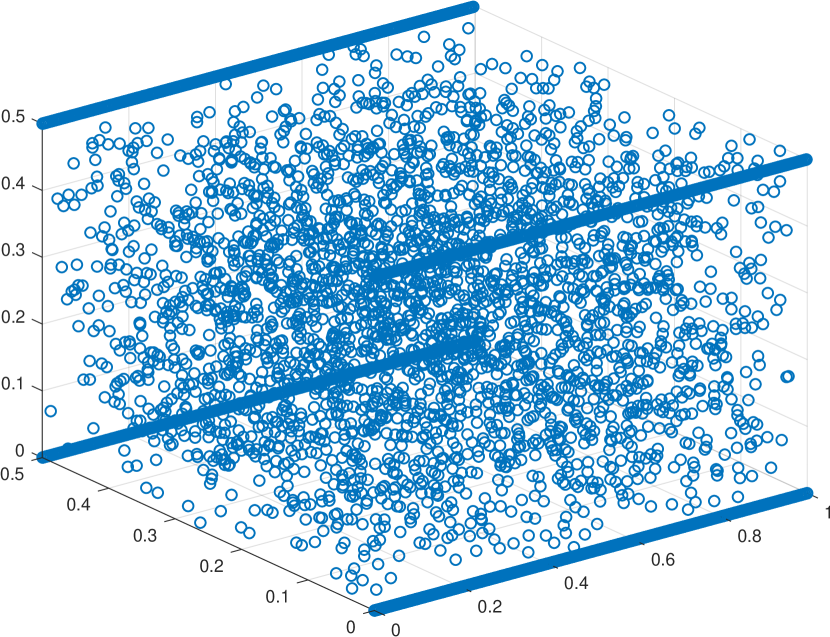
Refer to caption
(a) Four clusters in [0,1]×[0,12]×[0,12]01012012[0,1]\times[0,\frac{1}{2}]\times[0,\frac{1}{2}].
Refer to caption
(b) Corresponding pairwise LLPD, sorted.
Refer to caption
(c) Corresponding pairwise 2superscript2\ell^{2} distances, sorted.
Figure 5: (a) The clusters are on edges of the rectangular prism so that the pairwise LLPDs between the clusters is at least 1. The interior is filled with noise points. Each cluster has 3000 points, as does the interior noise region. (b) The sorted ρsubscript𝜌\rho_{\ell\ell} plot shows within-cluster LLPDs in green, between-cluster LLPDs in blue, and LLPDs involving noise points in yellow. There is a clear phase transition between the within-cluster and between-cluster LLPDs. This empirical observation can be compared with the theoretical guarantees of Theorems 4.4 and 4.5. Setting t=.01𝑡.01t=.01 in those theorems yield corresponding maximum within-cluster LLPD (shown with the solid red line) and minimum between-cluster distance (shown with the dashed red line). The empirical results confirm our theoretical guarantees. Notice moreover that there is no clear separation between the Euclidean distances, which are shown in (c). This illustrates the challenges faced by classical spectral clustering, compared to LLPD spectral clustering, for this dataset.

5 Performance Guarantees for Ultrametric and LLPD Spectral Clustering

In this section we first derive performance guarantees for spectral clustering with any ultrametric. We show that when the data consists of cluster cores surrounded by noise, the weight matrix W𝑊W used in spectral clustering is, for a certain range of scales σ𝜎\sigma, approximately block diagonal with constant blocks. In this range of σ𝜎\sigma, the number of clusters can be inferred from the maximal eigengap of LSYMsubscript𝐿SYM{L_{\text{SYM}}}, and spectral clustering achieves high labeling accuracy. On the other hand, for Euclidean spectral clustering it is hard to choose a scale parameter that is simultaneously large enough to guarantee a strong connection between every pair of points in the same cluster and small enough to produce weak connections between clusters (and even when possible the shape (e.g. elongation) of clusters affects the ability to identify the correct clusters). The resulting Euclidean weight matrix is not approximately block diagonal for any choice of σ𝜎\sigma, and the eigengap of LSYMsubscript𝐿SYM{L_{\text{SYM}}} becomes uninformative and the labeling accuracy potentially poor. Moreover, using an ultrametric for spectral clustering leads to direct lower bounds on the degree of noise points, since if a noise point is close to any cluster point, it is close to all points in the given cluster. It is well-known that spectral clustering is unreliable for points of low degree and in this case LSYMsubscript𝐿SYM{L_{\text{SYM}}} may have arbitrarily many small eigenvalues (Von Luxburg, 2007).

After proving results for general ultrametrics, we derive specific performance guarantees for LLPD spectral clustering on the LDLN data model. We remove low density points by considering each point’s LLPD-nearest neighbor distances, then derive bounds on the eigengap and labeling accuracy which hold even in the presence of noise points with weak connections to the clusters. We prove there is a large range of values of both the thresholding and scale parameter for which we correctly recover the clusters, illustrating that LLPD spectral clustering is robust to the choice of parameters and presence of noise. In particular, when the clusters have a very low-dimensional structure and the noise is very high-dimensional, that is, when dDmuch-less-than𝑑𝐷d\ll D, an enormous amount of noise points can be tolerated. Throughout this section, we use the notation established in Subsection 2.3.

5.1 Ultrametric Spectral Clustering

Let ρ:D×D[0,):𝜌superscript𝐷superscript𝐷0\rho:\mathbb{R}^{D}\times\mathbb{R}^{D}\rightarrow[0,\infty) be an ultrametric; see (2.1). We analyze LSYMsubscript𝐿SYM{L_{\text{SYM}}} under the assumptions of the following cluster model. As will be seen in Subsection 5.2, this cluster model holds for data drawn from the LDLN data model with the LLPD ultrametric, but it may be of interest in other regimes and for other ultrametrics. The model assumes there are K𝐾K sets forming cluster cores and each cluster core has a halo of noise points surrounding it; for 1lK1𝑙𝐾1\leq l\leq K, Alsubscript𝐴𝑙A_{l} denotes the cluster core and Clsubscript𝐶𝑙C_{l} the associated halo of noise points. For LDLN data, the parameter ϵsepsubscriptitalic-ϵsep\epsilon_{\mathrm{sep}} corresponds to the minimal between cluster distance after denoising.

Assumption 1 (Ultrametric Cluster Model)

For 1lK1𝑙𝐾1\leq l\leq K, assume Alsubscript𝐴𝑙A_{l} and Clsubscript𝐶𝑙C_{l} are disjoint finite sets, and let Al~=AlCl~subscript𝐴𝑙subscript𝐴𝑙subscript𝐶𝑙\tilde{A_{l}}=A_{l}\cup C_{l}. Let N=|lA~l|𝑁subscript𝑙subscript~𝐴𝑙N=|\cup_{l}\tilde{A}_{l}|. Assume that for some ϵinθ<ϵsepsubscriptitalic-ϵin𝜃subscriptitalic-ϵsep\epsilon_{\mathrm{in}}\leq\theta<\epsilon_{\mathrm{sep}}:

ρ(xil,xjl)𝜌subscriptsuperscript𝑥𝑙𝑖subscriptsuperscript𝑥𝑙𝑗\displaystyle\rho(x^{l}_{i},x^{l}_{j}) ϵinabsentsubscriptitalic-ϵin\displaystyle\leq\epsilon_{\mathrm{in}} xil,xjlAl,1lK,formulae-sequencefor-allsubscriptsuperscript𝑥𝑙𝑖subscriptsuperscript𝑥𝑙𝑗subscript𝐴𝑙1𝑙𝐾\displaystyle\forall x^{l}_{i},x^{l}_{j}\in A_{l},1\leq l\leq K, (5.1)
ϵin<ρ(xil,xjl)subscriptitalic-ϵin𝜌subscriptsuperscript𝑥𝑙𝑖subscriptsuperscript𝑥𝑙𝑗\displaystyle\epsilon_{\mathrm{in}}<\rho(x^{l}_{i},x^{l}_{j}) θabsent𝜃\displaystyle\leq\theta xilAl,xjlCl,1lK,formulae-sequencefor-allsubscriptsuperscript𝑥𝑙𝑖subscript𝐴𝑙formulae-sequencesubscriptsuperscript𝑥𝑙𝑗subscript𝐶𝑙1𝑙𝐾\displaystyle\forall x^{l}_{i}\in A_{l},x^{l}_{j}\in C_{l},1\leq l\leq K, (5.2)
ρ(xil,xjs)𝜌subscriptsuperscript𝑥𝑙𝑖subscriptsuperscript𝑥𝑠𝑗\displaystyle\rho(x^{l}_{i},x^{s}_{j}) ϵsepabsentsubscriptitalic-ϵsep\displaystyle\geq\epsilon_{\mathrm{sep}} xilA~l,xjsA~s,1lsK.formulae-sequencefor-allsubscriptsuperscript𝑥𝑙𝑖subscript~𝐴𝑙formulae-sequencesubscriptsuperscript𝑥𝑠𝑗subscript~𝐴𝑠1𝑙𝑠𝐾\displaystyle\forall x^{l}_{i}\in\tilde{A}_{l},x^{s}_{j}\in\tilde{A}_{s},1\leq l\neq s\leq K. (5.3)

Moreover, let ζN=max1lKN|A~l|.subscript𝜁𝑁subscript1𝑙𝐾𝑁subscript~𝐴𝑙\zeta_{N}=\max_{1\leq l\leq K}\frac{N}{|\tilde{A}_{l}|}.

Theorem 5.2 shows that under Assumption 1, the maximal eigengap of LSYMsubscript𝐿SYM{L_{\text{SYM}}} corresponds to the number of clusters K𝐾K and spectral clustering with K𝐾K principal eigenvectors achieves perfect labeling accuracy. The label accuracy result is obtained by showing the spectral embedding with K𝐾K principal eigenvectors is a perfect representation of the sets A~lsubscript~𝐴𝑙\tilde{A}_{l}, as defined in Vu (2018).

Definition 5.1 (Perfect Representation)

A clustering representation is perfect if there exists an r>0𝑟0r>0 such that

  • \cdot

    Vertices in the same cluster have distance at most r𝑟r.

  • \cdot

    Vertices from different clusters have distance at least 4r4𝑟4r from each other.

There are multiple clustering algorithms which are guaranteed to perfectly recover the labels of A~lsubscript~𝐴𝑙\tilde{A}_{l} from a perfect representation, including K𝐾K-means with furthest point initialization and single linkage clustering. Again following the terminology in Vu (2018), we will refer to all such clustering algorithms as clustering by distances. The proof of Theorem 5.2 is in Appendix B.

Theorem 5.2

Assume the ultrametric cluster model. Then λK+1λKsubscript𝜆𝐾1subscript𝜆𝐾\lambda_{K+1}-\lambda_{K} is the largest gap in the eigenvalues of LSYM(lA~l,ρ,fσ)subscript𝐿SYMsubscript𝑙subscript~𝐴𝑙𝜌subscript𝑓𝜎L_{\text{SYM}}(\cup_{l}\tilde{A}_{l},\rho,f_{\sigma}) provided

1212\displaystyle\frac{1}{2}\ 5(1fσ(ϵin))Cluster Coherence+6ζNfσ(ϵsep)Cluster Separation+4(1fσ(θ))Noise+β,absentCluster Coherence51subscript𝑓𝜎subscriptitalic-ϵinlimit-fromCluster Separation6subscript𝜁𝑁subscript𝑓𝜎subscriptitalic-ϵsepNoise41subscript𝑓𝜎𝜃𝛽\displaystyle\geq\ \underset{\textbf{Cluster Coherence}}{\underbrace{5(1-f_{\sigma}(\epsilon_{\mathrm{in}}))}}\ \ +\ \underset{\textbf{Cluster Separation}}{\underbrace{6\zeta_{N}f_{\sigma}(\epsilon_{\mathrm{sep}})}}\ +\ \ \underset{\textbf{Noise}}{\underbrace{4(1-f_{\sigma}(\theta))}}\ +\ \beta\ , (5.4)

where β=O((1fσ(ϵin))2+ζN2fσ(ϵsep)2+(1fσ(θ))2)𝛽𝑂superscript1subscript𝑓𝜎subscriptitalic-ϵin2superscriptsubscript𝜁𝑁2subscript𝑓𝜎superscriptsubscriptitalic-ϵsep2superscript1subscript𝑓𝜎𝜃2\beta=O((1-f_{\sigma}(\epsilon_{\mathrm{in}}))^{2}+\zeta_{N}^{2}f_{\sigma}(\epsilon_{\mathrm{sep}})^{2}+(1-f_{\sigma}(\theta))^{2}) denotes higher-order terms. Moreover, if

CK3ζN2(1fσ(ϵin))+ζNfσ(ϵsep)+(1fσ(θ))+β,𝐶superscript𝐾3superscriptsubscript𝜁𝑁21subscript𝑓𝜎subscriptitalic-ϵinsubscript𝜁𝑁subscript𝑓𝜎subscriptitalic-ϵsep1subscript𝑓𝜎𝜃𝛽\displaystyle\frac{C}{K^{3}\zeta_{N}^{2}}\geq(1-f_{\sigma}(\epsilon_{\mathrm{in}}))+\zeta_{N}f_{\sigma}(\epsilon_{\mathrm{sep}})+(1-f_{\sigma}(\theta))+\beta\ , (5.5)

where C𝐶C is an absolute constant, then clustering by distances on the K𝐾K principal eigenvectors of LSYM(lA~l,ρ,fσ)subscript𝐿SYMsubscript𝑙subscript~𝐴𝑙𝜌subscript𝑓𝜎{L_{\text{SYM}}}(\cup_{l}\tilde{A}_{l},\rho,f_{\sigma}) perfectly recovers the cluster labels.

For condition (5.4) to hold, the following three terms must all be small:

  • Cluster Coherence: This term is minimized by choosing σ𝜎\sigma large so that fσ(ϵin)1subscript𝑓𝜎subscriptitalic-ϵin1f_{\sigma}(\epsilon_{\mathrm{in}})\approx 1; the larger the scale parameter, the stronger the within-cluster connections.

  • Cluster Separation: This term is minimized by choosing σ𝜎\sigma small so that fσ(ϵsep)0subscript𝑓𝜎subscriptitalic-ϵsep0f_{\sigma}(\epsilon_{\mathrm{sep}})\approx 0; the smaller the scale parameter, the weaker the between-cluster connections. Note ζNsubscript𝜁𝑁\zeta_{N} is minimized when clusters are balanced, in which case ζN=Ksubscript𝜁𝑁𝐾\zeta_{N}=K.

  • Noise: This term is minimized by choosing σ𝜎\sigma large, so that once again fσ(θ)1subscript𝑓𝜎𝜃1f_{\sigma}(\theta)\approx 1. When the scale parameter is large, noise points around the cluster will be well connected to their designated cluster.

  • Higher Order Terms: This term consists of terms that are quadratic in (1fσ(ϵin)),fσ(ϵsep),(1fσ(θ))1subscript𝑓𝜎subscriptitalic-ϵinsubscript𝑓𝜎subscriptitalic-ϵsep1subscript𝑓𝜎𝜃(1-f_{\sigma}(\epsilon_{\mathrm{in}})),f_{\sigma}(\epsilon_{\mathrm{sep}}),(1-f_{\sigma}(\theta)), which are small in our regime of interest.

Solving for the scale parameter σ𝜎\sigma will yield a range of σ𝜎\sigma values where the eigengap statistic is informative; this is done in Corollary 5.7 for LLPD spectral clustering on the LDLN data model.

Condition (5.5) guarantees that clustering the LLPD spectral embedding results in perfect label accuracy, and requires a stronger scaling with respect to K𝐾K than Condition (5.4), as when ζN=O(K)subscript𝜁𝑁𝑂𝐾\zeta_{N}=O(K) there is an additional factor of K5superscript𝐾5K^{-5} on the left hand side of the inequality. Determining whether this scaling in K𝐾K is optimal is a topic of ongoing research, though the present article is more concerned with scaling in n,d,𝑛𝑑n,d, and D𝐷D. Condition (5.5) in fact guarantees perfect accuracy for clustering by distances on the spectral embedding regardless of whether the K𝐾K principal eigenvectors of LSYMsubscript𝐿SYM{L_{\text{SYM}}} are row-normalized or not. Row normalization is proposed in Ng et al. (2002) and generally results in better clustering results when some points have small degree (Von Luxburg, 2007); however it is not needed here because the properties of LLPD cause all points to have similar degree.

Remark 5.3

One can also derive a label accuracy result by applying Theorem 2 from Ng et al. (2002), restated in Arias-Castro (2011), to show the spectral embedding satisfies the so-called orthogonal cone property (OCP) (Schiebinger et al., 2015). Indeed, let {ϕk}k=1Ksuperscriptsubscriptsubscriptitalic-ϕ𝑘𝑘1𝐾\{\phi_{k}\}_{k=1}^{K} be the principal eigenvectors of LSYMsubscript𝐿SYM{L_{\text{SYM}}}. The OCP guarantees that in the representation x{ϕk(x)}k=1Kmaps-to𝑥superscriptsubscriptsubscriptitalic-ϕ𝑘𝑥𝑘1𝐾x\mapsto\{\phi_{k}(x)\}_{k=1}^{K}, distinct clusters localize in nearly orthogonal directions, not too far from the origin. Proposition 1 from Schiebinger et al. (2015) can then be applied to conclude K𝐾K-means on the spectral embedding achieves high accuracy. Specifically, if (5.4) is satisfied, then with probability at least 1t1𝑡1-t, K𝐾K-means on the K𝐾K principal eigenvectors of LSYM(lA~l,ρ,fσ)subscript𝐿SYMsubscript𝑙subscript~𝐴𝑙𝜌subscript𝑓𝜎{L_{\text{SYM}}}(\cup_{l}\tilde{A}_{l},\rho,f_{\sigma}) achieves accuracy at least 1cK9ζN3(fσ(ϵsep)2+β)t1𝑐superscript𝐾9superscriptsubscript𝜁𝑁3subscript𝑓𝜎superscriptsubscriptitalic-ϵsep2𝛽𝑡1-\frac{cK^{9}\zeta_{N}^{3}(f_{\sigma}(\epsilon_{\mathrm{sep}})^{2}+\beta)}{t} where c𝑐c is an absolute constant and β𝛽\beta denotes higher order terms. This approach results in a less restrictive scaling for 1fσ(ϵin),fσ(ϵsep)1subscript𝑓𝜎subscriptitalic-ϵinsubscript𝑓𝜎subscriptitalic-ϵsep1-f_{\sigma}(\epsilon_{\mathrm{in}}),f_{\sigma}(\epsilon_{\mathrm{sep}}) in terms of K,ζN𝐾subscript𝜁𝑁K,\zeta_{N} than given in Condition (5.5), but does not guarantee perfect accuracy, and also requires row normalization of the spectral embedding as proposed in Ng et al. (2002). The argument using this approach to proving cluster accuracy is not discussed in this article, for reasons of space and as to not introduce additional excessive notation.

5.2 LLPD Spectral Clustering with k𝑘kNN LLPD Thresholding

We now return to the LDLN data model defined in Subsection 3.2 and show that it gives rise to the ultrametric cluster model described in Assumption 1 when combined with the LLPD metric. Theorem 5.2 can thus be applied to derive performance guarantees for LLPD spectral clustering on the LDLN data model. All of the notation and assumptions established in Subsection 3.2 hold throughout Subsection 5.2.

5.2.1 Thresholding

Before applying spectral clustering, we denoise the data by removing any points having sufficiently large LLPD to their knsethsuperscriptsubscript𝑘nseth{k_{\text{nse}}}^{\!\!\!\!\!\text{th}} LLPD-nearest neighbor. Motivated by the sharp phase transition illustrated in Subsection 4.4, we choose a threshold θ𝜃\theta and discard a point xX𝑥𝑋x\in X if βknse(x,X)>θsubscript𝛽subscript𝑘nse𝑥𝑋𝜃\beta_{{k_{\text{nse}}}}(x,X)>\theta. Note that the definition of ϵnsesubscriptitalic-ϵnse\epsilon_{\mathrm{nse}} guarantees that we can never have a group of more than knsesubscript𝑘nse{k_{\text{nse}}} noise points where all pairwise LLPD are smaller than ϵnsesubscriptitalic-ϵnse\epsilon_{\mathrm{nse}}, because if we did there would be a point xX~𝑥~𝑋x\in\tilde{X} with βknse(x,X~)<ϵnsesubscript𝛽subscript𝑘nse𝑥~𝑋subscriptitalic-ϵnse\beta_{{k_{\text{nse}}}}(x,\tilde{X})<\epsilon_{\mathrm{nse}}. Thus if ϵinθ<ϵnsesubscriptitalic-ϵin𝜃subscriptitalic-ϵnse\epsilon_{\mathrm{in}}\leq\theta<\epsilon_{\mathrm{nse}} then, after thresholding, the data will consist of the cluster cores Xlsubscript𝑋𝑙X_{l} with θ𝜃\theta-groups of at most knsesubscript𝑘nse{k_{\text{nse}}} noise points emanating from the cluster cores, where a θ𝜃\theta-group denotes a set of points where the LLPD between all pairs of points in the group is at most θ𝜃\theta.

We assume LLPD is re-computed on the denoised data set XNsubscript𝑋𝑁X_{N}, whose cardinality we define to be N𝑁N, and let ρXNsubscriptsuperscript𝜌subscript𝑋𝑁\rho^{X_{N}}_{\ell\ell} denote the corresponding LLPD metric. The points remaining after thresholding consist of the sets A~lsubscript~𝐴𝑙\tilde{A}_{l}, where

Al={xiXl}{xiX~|ρ(xi,xj)ϵin for some xjXl},Cl={xiX~|ϵin<ρ(xi,xj)θ for some xjXl},A~l=AlCl={xiXl}{xiX~|ρ(xi,xj)θ for some xjXl}.subscript𝐴𝑙absentsubscript𝑥𝑖subscript𝑋𝑙conditional-setsubscript𝑥𝑖~𝑋subscript𝜌subscript𝑥𝑖subscript𝑥𝑗subscriptitalic-ϵin for some subscript𝑥𝑗subscript𝑋𝑙subscript𝐶𝑙absentconditional-setsubscript𝑥𝑖~𝑋subscriptitalic-ϵinsubscript𝜌subscript𝑥𝑖subscript𝑥𝑗𝜃 for some subscript𝑥𝑗subscript𝑋𝑙subscript~𝐴𝑙absentsubscript𝐴𝑙subscript𝐶𝑙subscript𝑥𝑖subscript𝑋𝑙conditional-setsubscript𝑥𝑖~𝑋subscript𝜌subscript𝑥𝑖subscript𝑥𝑗𝜃 for some subscript𝑥𝑗subscript𝑋𝑙\begin{array}[]{r@{}l}A_{l}{}&=\{x_{i}\in X_{l}\}\cup\{x_{i}\in\tilde{X}\ |\ \rho_{\ell\ell}(x_{i},x_{j})\leq\epsilon_{\mathrm{in}}\text{ for some }x_{j}\in X_{l}\},\\[2.84544pt] C_{l}{}&=\{x_{i}\in\tilde{X}\ |\ \epsilon_{\mathrm{in}}<\rho_{\ell\ell}(x_{i},x_{j})\leq\theta\text{ for some }x_{j}\in X_{l}\},\\[2.84544pt] \tilde{A}_{l}{}&=A_{l}\cup C_{l}=\{x_{i}\in X_{l}\}\cup\{x_{i}\in\tilde{X}\ |\ \rho_{\ell\ell}(x_{i},x_{j})\leq\theta\text{ for some }x_{j}\in X_{l}\}.\end{array} (5.6)

The cluster core Alsubscript𝐴𝑙A_{l} consists of the points Xlsubscript𝑋𝑙X_{l} plus any noise points in X~~𝑋\tilde{X} that are indistinguishable from Xlsubscript𝑋𝑙X_{l}, being within the maximal within-cluster LLPD of Xlsubscript𝑋𝑙X_{l}. The set Clsubscript𝐶𝑙C_{l} consists of the noise points in X~~𝑋\tilde{X} that are θ𝜃\theta-close to Xlsubscript𝑋𝑙X_{l} in LLPD.

5.2.2 Supporting Lemmata

The following two lemmata are needed to prove Theorem 5.6, the main result of this subsection. The first one guarantees that the sets defined in (5.6) describe exactly the points which survive thresholding, that is XN=lA~lsubscript𝑋𝑁subscript𝑙subscript~𝐴𝑙X_{N}=\cup_{l}\tilde{A}_{l}.

Lemma 5.4

Assume the LDLN data model and assumptions, and let A~lsubscript~𝐴𝑙\tilde{A}_{l} be as in (5.6). If knse<nminsubscript𝑘nsesubscript𝑛min{k_{\text{nse}}}<n_{\text{min}}, ϵinθ<ϵnsesubscriptitalic-ϵin𝜃subscriptitalic-ϵnse\epsilon_{\mathrm{in}}\leq\theta<\epsilon_{\mathrm{nse}}, then βknse(x,X)θsubscript𝛽subscript𝑘nse𝑥𝑋𝜃\beta_{{k_{\text{nse}}}}(x,X)\leq\theta if and only if xA~l𝑥subscript~𝐴𝑙x\in\tilde{A}_{l} for some 1lK1𝑙𝐾1\leq l\leq K.

Proof  Assume βknse(x,X)θsubscript𝛽subscript𝑘nse𝑥𝑋𝜃\beta_{{k_{\text{nse}}}}(x,X)\leq\theta. If xlXl𝑥subscript𝑙subscript𝑋𝑙x\in\cup_{l}X_{l}, then clearly xlA~l𝑥subscript𝑙subscript~𝐴𝑙x\in\cup_{l}\tilde{A}_{l}, so assume xX~𝑥~𝑋x\in\tilde{X}. We claim there exists some ylXl𝑦subscript𝑙subscript𝑋𝑙y\in\cup_{l}X_{l} such that ρ(x,y)θsubscript𝜌𝑥𝑦𝜃\rho_{\ell\ell}(x,y)\leq\theta. Suppose not; then there exist knsesubscript𝑘nse{k_{\text{nse}}} points {xi}i=1knsesuperscriptsubscriptsubscript𝑥𝑖𝑖1subscript𝑘nse\{x_{i}\}_{i=1}^{{k_{\text{nse}}}} in X~~𝑋\tilde{X} distinct from x𝑥x with ρ(x,xi)θsubscript𝜌𝑥subscript𝑥𝑖𝜃\rho_{\ell\ell}(x,x_{i})\leq\theta; thus ϵnseθsubscriptitalic-ϵnse𝜃\epsilon_{\mathrm{nse}}\leq\theta, a contradiction. Hence, there exists yXl𝑦subscript𝑋𝑙y\in X_{l} such that ρ(x,y)θsubscript𝜌𝑥𝑦𝜃\rho_{\ell\ell}(x,y)\leq\theta and xA~l𝑥subscript~𝐴𝑙x\in\tilde{A}_{l}.
Now assume xA~l𝑥subscript~𝐴𝑙x\in\tilde{A}_{l} for some 1lK1𝑙𝐾1\leq l\leq K. Then clearly there exists ylXl𝑦subscript𝑙subscript𝑋𝑙y\in\cup_{l}X_{l} with ρ(x,y)θsubscript𝜌𝑥𝑦𝜃\rho_{\ell\ell}(x,y)\leq\theta. Since ϵin<θsubscriptitalic-ϵin𝜃\epsilon_{\mathrm{in}}<\theta, x𝑥x is within LLPD θ𝜃\theta of all points in Xlsubscript𝑋𝑙X_{l}, and since knse<nmin,βknse(x,X)βnmin(x,X)θformulae-sequencesubscript𝑘nsesubscript𝑛minsubscript𝛽subscript𝑘nse𝑥𝑋subscript𝛽subscript𝑛min𝑥𝑋𝜃{k_{\text{nse}}}<n_{\text{min}},\beta_{{k_{\text{nse}}}}(x,X)\leq\beta_{n_{\text{min}}}(x,X)\leq\theta.  

Next we show that when there is sufficient separation between the cluster cores, the LLPD between any two points in distinct clusters is bounded by δ/2𝛿2\delta/2, and thus the assumptions of Theorem 5.2 will be satisfied with ϵsep=δ/2subscriptitalic-ϵsep𝛿2\epsilon_{\mathrm{sep}}=\delta/2.

Lemma 5.5

Assume the LDLN data model and assumptions, and assume ϵinθ<ϵnseδ/(4knse)subscriptitalic-ϵin𝜃subscriptitalic-ϵnse𝛿4subscript𝑘nse\epsilon_{\mathrm{in}}\leq\theta<\epsilon_{\mathrm{nse}}\wedge\delta/(4{k_{\text{nse}}}), Al,Cl,A~lsubscript𝐴𝑙subscript𝐶𝑙subscript~𝐴𝑙A_{l},C_{l},\tilde{A}_{l} as defined in (5.6), and knse<nmin.subscript𝑘nsesubscript𝑛min{k_{\text{nse}}}<n_{\text{min}}. Then Assumption 1 is satisfied with ρ=ρXN𝜌subscriptsuperscript𝜌subscript𝑋𝑁\rho=\rho^{X_{N}}_{\ell\ell}, ϵsep=δ/2subscriptitalic-ϵsep𝛿2\epsilon_{\mathrm{sep}}=\delta/2.

Proof  First note that if xAl𝑥subscript𝐴𝑙x\in A_{l}, then ρ(x,y)ϵinsubscript𝜌𝑥𝑦subscriptitalic-ϵin\rho_{\ell\ell}(x,y)\leq\epsilon_{\mathrm{in}} for all yXl𝑦subscript𝑋𝑙y\in X_{l}, and thus xCl𝑥subscript𝐶𝑙x\notin C_{l}, so Alsubscript𝐴𝑙A_{l} and Clsubscript𝐶𝑙C_{l} are disjoint.

Let xil,xjlAlsubscriptsuperscript𝑥𝑙𝑖subscriptsuperscript𝑥𝑙𝑗subscript𝐴𝑙x^{l}_{i},x^{l}_{j}\in A_{l}. Then there exists yi,yjXlsubscript𝑦𝑖subscript𝑦𝑗subscript𝑋𝑙y_{i},y_{j}\in X_{l} with ρ(xil,yi)ϵinsubscript𝜌subscriptsuperscript𝑥𝑙𝑖subscript𝑦𝑖subscriptitalic-ϵin\rho_{\ell\ell}(x^{l}_{i},y_{i})\leq\epsilon_{\mathrm{in}} and ρ(xjl,yj)ϵinsubscript𝜌subscriptsuperscript𝑥𝑙𝑗subscript𝑦𝑗subscriptitalic-ϵin\rho_{\ell\ell}(x^{l}_{j},y_{j})\leq\epsilon_{\mathrm{in}}, so ρ(xil,xjl)ρ(xil,yi)ρ(yi,yj)ρ(yj,xjl)ϵinsubscript𝜌subscriptsuperscript𝑥𝑙𝑖subscriptsuperscript𝑥𝑙𝑗subscript𝜌subscriptsuperscript𝑥𝑙𝑖subscript𝑦𝑖subscript𝜌subscript𝑦𝑖subscript𝑦𝑗subscript𝜌subscript𝑦𝑗subscriptsuperscript𝑥𝑙𝑗subscriptitalic-ϵin\rho_{\ell\ell}(x^{l}_{i},x^{l}_{j})\leq\rho_{\ell\ell}(x^{l}_{i},y_{i})\vee\rho_{\ell\ell}(y_{i},y_{j})\vee\rho_{\ell\ell}(y_{j},x^{l}_{j})\leq\epsilon_{\mathrm{in}}. Since xil,xjlsubscriptsuperscript𝑥𝑙𝑖subscriptsuperscript𝑥𝑙𝑗x^{l}_{i},x^{l}_{j} were arbitrary, ρ(xil,xjl)ϵinsubscript𝜌subscriptsuperscript𝑥𝑙𝑖subscriptsuperscript𝑥𝑙𝑗subscriptitalic-ϵin\rho_{\ell\ell}(x^{l}_{i},x^{l}_{j})\leq\epsilon_{\mathrm{in}} for all xil,xjlAlsubscriptsuperscript𝑥𝑙𝑖subscriptsuperscript𝑥𝑙𝑗subscript𝐴𝑙x^{l}_{i},x^{l}_{j}\in A_{l}. We now show that in fact ρXN(xil,xjl)ϵinsubscriptsuperscript𝜌subscript𝑋𝑁subscriptsuperscript𝑥𝑙𝑖subscriptsuperscript𝑥𝑙𝑗subscriptitalic-ϵin\rho^{X_{N}}_{\ell\ell}(x^{l}_{i},x^{l}_{j})\leq\epsilon_{\mathrm{in}}. Suppose not. Since ρ(xil,xjl)ϵinsubscript𝜌subscriptsuperscript𝑥𝑙𝑖subscriptsuperscript𝑥𝑙𝑗subscriptitalic-ϵin\rho_{\ell\ell}(x^{l}_{i},x^{l}_{j})\leq\epsilon_{\mathrm{in}}, there exists a path in X𝑋X from xilsubscriptsuperscript𝑥𝑙𝑖x^{l}_{i} to xjlsubscriptsuperscript𝑥𝑙𝑗x^{l}_{j} with all legs bounded by ϵinsubscriptitalic-ϵin\epsilon_{\mathrm{in}}. Since ρXN(xil,xjl)>ϵinsubscriptsuperscript𝜌subscript𝑋𝑁subscriptsuperscript𝑥𝑙𝑖subscriptsuperscript𝑥𝑙𝑗subscriptitalic-ϵin\rho^{X_{N}}_{\ell\ell}(x^{l}_{i},x^{l}_{j})>\epsilon_{\mathrm{in}}, one of the points along this path must have been removed by thresholding, i.e. there exists y𝑦y on the path with βknse(y,X)>θsubscript𝛽subscript𝑘nse𝑦𝑋𝜃\beta_{{k_{\text{nse}}}}(y,X)>\theta. But then for all xlAlsuperscript𝑥𝑙subscript𝐴𝑙x^{l}\in A_{l}, ρ(y,xl)ρ(y,xil)ρ(xil,xl)ϵinsubscript𝜌𝑦superscript𝑥𝑙subscript𝜌𝑦superscriptsubscript𝑥𝑖𝑙subscript𝜌superscriptsubscript𝑥𝑖𝑙superscript𝑥𝑙subscriptitalic-ϵin\rho_{\ell\ell}(y,x^{l})\leq\rho_{\ell\ell}(y,x_{i}^{l})\vee\rho_{\ell\ell}(x_{i}^{l},x^{l})\leq\epsilon_{\mathrm{in}}, so βknse(y,X)ϵinsubscript𝛽subscript𝑘nse𝑦𝑋subscriptitalic-ϵin\beta_{{k_{\text{nse}}}}(y,X)\leq\epsilon_{\mathrm{in}} since knse<nminsubscript𝑘nsesubscript𝑛min{k_{\text{nse}}}<n_{\text{min}}; contradiction.

Let xilAl,xjlClformulae-sequencesubscriptsuperscript𝑥𝑙𝑖subscript𝐴𝑙subscriptsuperscript𝑥𝑙𝑗subscript𝐶𝑙x^{l}_{i}\in A_{l},x^{l}_{j}\in C_{l}. Then there exist points yi,yjXlsubscript𝑦𝑖subscript𝑦𝑗subscript𝑋𝑙y_{i},y_{j}\in X_{l} such that ρ(xil,yi)ϵinsubscript𝜌subscriptsuperscript𝑥𝑙𝑖subscript𝑦𝑖subscriptitalic-ϵin\rho_{\ell\ell}(x^{l}_{i},y_{i})\leq\epsilon_{\mathrm{in}} and ϵin<ρ(xjl,yj)θsubscriptitalic-ϵinsubscript𝜌subscriptsuperscript𝑥𝑙𝑗subscript𝑦𝑗𝜃\epsilon_{\mathrm{in}}<\rho_{\ell\ell}(x^{l}_{j},y_{j})\leq\theta. Thus ρ(xil,xjl)ρ(xil,yi)ρ(yi,yj)ρ(yj,xjl)ϵinϵinθ=θ.subscript𝜌subscriptsuperscript𝑥𝑙𝑖subscriptsuperscript𝑥𝑙𝑗subscript𝜌subscriptsuperscript𝑥𝑙𝑖subscript𝑦𝑖subscript𝜌subscript𝑦𝑖subscript𝑦𝑗subscript𝜌subscript𝑦𝑗subscriptsuperscript𝑥𝑙𝑗subscriptitalic-ϵinsubscriptitalic-ϵin𝜃𝜃\rho_{\ell\ell}(x^{l}_{i},x^{l}_{j})\leq\rho_{\ell\ell}(x^{l}_{i},y_{i})\vee\rho_{\ell\ell}(y_{i},y_{j})\vee\rho_{\ell\ell}(y_{j},x^{l}_{j})\leq\epsilon_{\mathrm{in}}\vee\epsilon_{\mathrm{in}}\vee\theta=\theta.

Now suppose ρ(xil,xjl)ϵinsubscript𝜌subscriptsuperscript𝑥𝑙𝑖subscriptsuperscript𝑥𝑙𝑗subscriptitalic-ϵin\rho_{\ell\ell}(x^{l}_{i},x^{l}_{j})\leq\epsilon_{\mathrm{in}}. Then ρ(xjl,yi)ρ(xjl,xil)ρ(xil,yi)ϵinsubscript𝜌subscriptsuperscript𝑥𝑙𝑗subscript𝑦𝑖subscript𝜌subscriptsuperscript𝑥𝑙𝑗subscriptsuperscript𝑥𝑙𝑖subscript𝜌subscriptsuperscript𝑥𝑙𝑖subscript𝑦𝑖subscriptitalic-ϵin\rho_{\ell\ell}(x^{l}_{j},y_{i})\leq\rho_{\ell\ell}(x^{l}_{j},x^{l}_{i})\vee\rho_{\ell\ell}(x^{l}_{i},y_{i})\leq\epsilon_{\mathrm{in}} so that xjlAlsubscriptsuperscript𝑥𝑙𝑗subscript𝐴𝑙x^{l}_{j}\in A_{l} since yiXlsubscript𝑦𝑖subscript𝑋𝑙y_{i}\in X_{l}; this is a contradiction since xjlClsubscriptsuperscript𝑥𝑙𝑗subscript𝐶𝑙x^{l}_{j}\in C_{l} and Alsubscript𝐴𝑙A_{l} and Clsubscript𝐶𝑙C_{l} are disjoint. We thus conclude ϵin<ρ(xil,xjl)θsubscriptitalic-ϵinsubscript𝜌subscriptsuperscript𝑥𝑙𝑖subscriptsuperscript𝑥𝑙𝑗𝜃\epsilon_{\mathrm{in}}<\rho_{\ell\ell}(x^{l}_{i},x^{l}_{j})\leq\theta. Since xil,xjlsubscriptsuperscript𝑥𝑙𝑖subscriptsuperscript𝑥𝑙𝑗x^{l}_{i},x^{l}_{j} were arbitrary, ϵin<ρ(xil,xjl)θsubscriptitalic-ϵinsubscript𝜌subscriptsuperscript𝑥𝑙𝑖subscriptsuperscript𝑥𝑙𝑗𝜃\epsilon_{\mathrm{in}}<\rho_{\ell\ell}(x^{l}_{i},x^{l}_{j})\leq\theta for all xilAl,xjlClformulae-sequencesubscriptsuperscript𝑥𝑙𝑖subscript𝐴𝑙subscriptsuperscript𝑥𝑙𝑗subscript𝐶𝑙x^{l}_{i}\in A_{l},x^{l}_{j}\in C_{l}. We now show in fact ϵin<ρXN(xil,xjl)θsubscriptitalic-ϵinsubscriptsuperscript𝜌subscript𝑋𝑁subscriptsuperscript𝑥𝑙𝑖subscriptsuperscript𝑥𝑙𝑗𝜃\epsilon_{\mathrm{in}}<\rho^{X_{N}}_{\ell\ell}(x^{l}_{i},x^{l}_{j})\leq\theta. Clearly, ϵin<ρ(xil,xjl)ρXN(xil,xjl)subscriptitalic-ϵinsubscript𝜌subscriptsuperscript𝑥𝑙𝑖subscriptsuperscript𝑥𝑙𝑗subscriptsuperscript𝜌subscript𝑋𝑁subscriptsuperscript𝑥𝑙𝑖subscriptsuperscript𝑥𝑙𝑗\epsilon_{\mathrm{in}}<\rho_{\ell\ell}(x^{l}_{i},x^{l}_{j})\leq\rho^{X_{N}}_{\ell\ell}(x^{l}_{i},x^{l}_{j}). Now suppose ρXN(xil,xjl)>θsubscriptsuperscript𝜌subscript𝑋𝑁subscriptsuperscript𝑥𝑙𝑖subscriptsuperscript𝑥𝑙𝑗𝜃\rho^{X_{N}}_{\ell\ell}(x^{l}_{i},x^{l}_{j})>\theta. Since ρ(xil,xjl)θsubscript𝜌subscriptsuperscript𝑥𝑙𝑖subscriptsuperscript𝑥𝑙𝑗𝜃\rho_{\ell\ell}(x^{l}_{i},x^{l}_{j})\leq\theta, there exists a path in X𝑋X from xilsubscriptsuperscript𝑥𝑙𝑖x^{l}_{i} to xjlsubscriptsuperscript𝑥𝑙𝑗x^{l}_{j} with all legs bounded by θ𝜃\theta. Since ρXN(xil,xjl)>θsubscriptsuperscript𝜌subscript𝑋𝑁subscriptsuperscript𝑥𝑙𝑖subscriptsuperscript𝑥𝑙𝑗𝜃\rho^{X_{N}}_{\ell\ell}(x^{l}_{i},x^{l}_{j})>\theta, one of the points along this path must have been removed by thresholding, i.e. there exists y𝑦y on the path with βknse(y,X)>θsubscript𝛽subscript𝑘nse𝑦𝑋𝜃\beta_{{k_{\text{nse}}}}(y,X)>\theta. But then for all xlA~lsuperscript𝑥𝑙subscript~𝐴𝑙x^{l}\in\tilde{A}_{l}, ρ(y,xl)ρ(y,xil)ρ(xil,xl)θsubscript𝜌𝑦superscript𝑥𝑙subscript𝜌𝑦superscriptsubscript𝑥𝑖𝑙subscript𝜌superscriptsubscript𝑥𝑖𝑙superscript𝑥𝑙𝜃\rho_{\ell\ell}(y,x^{l})\leq\rho_{\ell\ell}(y,x_{i}^{l})\vee\rho_{\ell\ell}(x_{i}^{l},x^{l})\leq\theta, so βknse(y,X)θsubscript𝛽subscript𝑘nse𝑦𝑋𝜃\beta_{{k_{\text{nse}}}}(y,X)\leq\theta since knse<nminsubscript𝑘nsesubscript𝑛min{k_{\text{nse}}}<n_{\text{min}}, which is a contradiction.

Finally, we show we can choose ϵsep=δ/2subscriptitalic-ϵsep𝛿2\epsilon_{\mathrm{sep}}=\delta/2, that is, ρXN(xil,xjs)δ/2subscriptsuperscript𝜌subscript𝑋𝑁subscriptsuperscript𝑥𝑙𝑖subscriptsuperscript𝑥𝑠𝑗𝛿2\rho^{X_{N}}_{\ell\ell}(x^{l}_{i},x^{s}_{j})\geq\delta/2 for all xilA~l,xjsA~s,lsformulae-sequencesubscriptsuperscript𝑥𝑙𝑖subscript~𝐴𝑙formulae-sequencesubscriptsuperscript𝑥𝑠𝑗subscript~𝐴𝑠𝑙𝑠x^{l}_{i}\in\tilde{A}_{l},x^{s}_{j}\in\tilde{A}_{s},l\neq s. We first verify that every point in A~lsubscript~𝐴𝑙\tilde{A}_{l} is within Euclidean distance θknse𝜃subscript𝑘nse\theta{k_{\text{nse}}} of a point in Xlsubscript𝑋𝑙X_{l}. Let xA~l𝑥subscript~𝐴𝑙x\in\tilde{A}_{l} and assume xX~𝑥~𝑋x\in\tilde{X} (otherwise there is nothing to show). Then there exists a point yXl𝑦subscript𝑋𝑙y\in X_{l} with ρ(x,y)θsubscript𝜌𝑥𝑦𝜃\rho_{\ell\ell}(x,y)\leq\theta, i.e. there exists a path of points from x𝑥x to y𝑦y with the length of all legs bounded by θ𝜃\theta. Note there can be at most knsesubscript𝑘nse{k_{\text{nse}}} consecutive noise points along this path, since otherwise we would have a zX~𝑧~𝑋z\in\tilde{X} with βknse(z,X~)θsubscript𝛽subscript𝑘nse𝑧~𝑋𝜃\beta_{{k_{\text{nse}}}}(z,\tilde{X})\leq\theta which contradicts ϵnse>θsubscriptitalic-ϵnse𝜃\epsilon_{\mathrm{nse}}>\theta. Let ysuperscript𝑦y^{*} be the last point in Xlsubscript𝑋𝑙X_{l} on this path. Since θ<δ/(4knse)<δ/(2knse+1)𝜃𝛿4subscript𝑘nse𝛿2subscript𝑘nse1\theta<\delta/(4{k_{\text{nse}}})<\delta/(2{k_{\text{nse}}}+1), dist(Xl,Xs)δ>2θknse+θdistsubscript𝑋𝑙subscript𝑋𝑠𝛿2𝜃subscript𝑘nse𝜃\text{dist}({X}_{l},{X}_{s})\geq\delta>2\theta{k_{\text{nse}}}+\theta, and the path cannot contain any points in Xs,lssubscript𝑋𝑠𝑙𝑠X_{s},l\neq s; thus the path from ysuperscript𝑦y^{*} to x𝑥x consists of at most knsesubscript𝑘nse{k_{\text{nse}}} points in X~~𝑋\tilde{X}, so xy2knseθsubscriptnorm𝑥superscript𝑦2subscript𝑘nse𝜃\|x-y^{*}\|_{2}\leq{k_{\text{nse}}}\theta. Thus: min1lsKdist(A~l,A~s)min1lsKdist(Xl,Xs)2θknseδ2θknse>δ/2subscript1𝑙𝑠𝐾distsubscript~𝐴𝑙subscript~𝐴𝑠subscript1𝑙𝑠𝐾distsubscript𝑋𝑙subscript𝑋𝑠2𝜃subscript𝑘nse𝛿2𝜃subscript𝑘nse𝛿2\min_{1\leq l\neq s\leq K}\text{dist}(\tilde{A}_{l},\tilde{A}_{s})\geq\min_{1\leq l\neq s\leq K}\text{dist}(X_{l},X_{s})-2\theta{k_{\text{nse}}}\geq\delta-2\theta{k_{\text{nse}}}>\delta/2 since θ<δ/(4knse)𝜃𝛿4subscript𝑘nse\theta<\delta/(4{k_{\text{nse}}}). Now by Lemma 5.4, there are no points outside of lA~lsubscript𝑙subscript~𝐴𝑙\cup_{l}\tilde{A}_{l} which survive thresholding, so we conclude ρXN(xil,xjs)δ/2subscriptsuperscript𝜌subscript𝑋𝑁subscriptsuperscript𝑥𝑙𝑖subscriptsuperscript𝑥𝑠𝑗𝛿2\rho^{X_{N}}_{\ell\ell}(x^{l}_{i},x^{s}_{j})\geq\delta/2 for all xilA~l,xjsA~sformulae-sequencesubscriptsuperscript𝑥𝑙𝑖subscript~𝐴𝑙subscriptsuperscript𝑥𝑠𝑗subscript~𝐴𝑠x^{l}_{i}\in\tilde{A}_{l},x^{s}_{j}\in\tilde{A}_{s}.  

5.2.3 Main Result

We now state our main result for LLPD spectral clustering with k𝑘kNN LLPD thresholding.

Theorem 5.6

Assume the LDLN data model and assumptions. For a chosen θ𝜃\theta and knsesubscript𝑘nse{k_{\text{nse}}}, perform thresholding at level θ𝜃\theta as above to obtain XNsubscript𝑋𝑁X_{N}, and assume knse<nminsubscript𝑘nsesubscript𝑛min{k_{\text{nse}}}<n_{\text{min}}, ϵinθ<ϵnseδ/(4knse)subscriptitalic-ϵin𝜃subscriptitalic-ϵnse𝛿4subscript𝑘nse\epsilon_{\mathrm{in}}\leq\theta<\epsilon_{\mathrm{nse}}\wedge\delta/(4{k_{\text{nse}}}). Then λK+1λKsubscript𝜆𝐾1subscript𝜆𝐾\lambda_{K+1}-\lambda_{K} is the largest gap in the eigenvalues of LSYM(XN,ρXN,fσ)subscript𝐿SYMsubscript𝑋𝑁subscriptsuperscript𝜌subscript𝑋𝑁subscript𝑓𝜎L_{\text{SYM}}(X_{N},\rho^{X_{N}}_{\ell\ell},f_{\sigma}) provided that

1212\displaystyle\frac{1}{2} 5(1fσ(ϵin))+6ζNfσ(δ/2)+4(1fσ(θ))+β,absent51subscript𝑓𝜎subscriptitalic-ϵin6subscript𝜁𝑁subscript𝑓𝜎𝛿241subscript𝑓𝜎𝜃𝛽\displaystyle\geq 5(1-f_{\sigma}(\epsilon_{\mathrm{in}}))+6\zeta_{N}f_{\sigma}(\delta/2)+4(1-f_{\sigma}(\theta))+\beta\ , (5.7)

and clustering by distances on the K𝐾K principal eigenvectors of LSYM(XN,ρXN,fσ)subscript𝐿SYMsubscript𝑋𝑁subscriptsuperscript𝜌subscript𝑋𝑁subscript𝑓𝜎L_{\text{SYM}}(X_{N},\rho^{X_{N}}_{\ell\ell},f_{\sigma}) perfectly recovers the cluster labels provided that

CK3ζN2(1fσ(ϵin))+ζNfσ(δ/2)+(1fσ(θ))+β,𝐶superscript𝐾3superscriptsubscript𝜁𝑁21subscript𝑓𝜎subscriptitalic-ϵinsubscript𝜁𝑁subscript𝑓𝜎𝛿21subscript𝑓𝜎𝜃𝛽\displaystyle\frac{C}{K^{3}\zeta_{N}^{2}}\geq(1-f_{\sigma}(\epsilon_{\mathrm{in}}))+\zeta_{N}f_{\sigma}(\delta/2)+(1-f_{\sigma}(\theta))+\beta\ ,

where β=O((1fσ(ϵin)2+ζN2fσ(δ/2)2+(1fσ(θ))2)\beta=O\left((1-f_{\sigma}(\epsilon_{\mathrm{in}})^{2}+\zeta_{N}^{2}f_{\sigma}(\delta/2)^{2}+(1-f_{\sigma}(\theta))^{2}\right) denotes higher-order terms and C𝐶C is an absolute constant. In addition, for nminsubscript𝑛n_{\min} large enough with probability at least 1O(nmin1)1𝑂superscriptsubscript𝑛11-O(n_{\min}^{-1}), ζN2ζn+3knseζθsubscript𝜁𝑁2subscript𝜁𝑛3subscript𝑘nsesubscript𝜁𝜃\zeta_{N}\leq 2\zeta_{n}+3{k_{\text{nse}}}\zeta_{\theta} for the LDLN data model balance parameters ζn,ζθsubscript𝜁𝑛subscript𝜁𝜃\zeta_{n},\zeta_{\theta}.

Proof  Define the sets Al,Cl,A~lsubscript𝐴𝑙subscript𝐶𝑙subscript~𝐴𝑙A_{l},C_{l},\tilde{A}_{l} as in (5.6). By Lemma 5.4, removing all points satisfying βknse(x,X)>θsubscript𝛽subscript𝑘nse𝑥𝑋𝜃\beta_{{k_{\text{nse}}}}(x,X)>\theta leaves us with exactly XN=lA~lsubscript𝑋𝑁subscript𝑙subscript~𝐴𝑙X_{N}=\cup_{l}\tilde{A}_{l}. By Lemma 5.5, all assumptions of Theorem 5.2 are satisfied for ultrametric ρXNsubscriptsuperscript𝜌subscript𝑋𝑁\rho^{X_{N}}_{\ell\ell} and we can apply Theorem 5.2 with ϵin,ϵnsesubscriptitalic-ϵinsubscriptitalic-ϵnse\epsilon_{\mathrm{in}},\epsilon_{\mathrm{nse}} as defined in Subsection 3.2 and ϵsep=δ/2subscriptitalic-ϵsep𝛿2\epsilon_{\mathrm{sep}}=\delta/2. All that remains is to verify the bound on ζNsubscript𝜁𝑁\zeta_{N}.

Recall A~l=Xl{xiX~|ρ(xi,xj)θ for some xjXl}subscript~𝐴𝑙subscript𝑋𝑙conditional-setsubscript𝑥𝑖~𝑋subscript𝜌subscript𝑥𝑖subscript𝑥𝑗𝜃 for some subscript𝑥𝑗subscript𝑋𝑙\tilde{A}_{l}=X_{l}\cup\{x_{i}\in\tilde{X}\ |\ \rho_{\ell\ell}(x_{i},x_{j})\leq\theta\text{ for some }x_{j}\in X_{l}\}; let mlsubscript𝑚𝑙m_{l} denote the cardinality of {xiX~|ρ(xi,xj)θ for some xjXl}conditional-setsubscript𝑥𝑖~𝑋subscript𝜌subscript𝑥𝑖subscript𝑥𝑗𝜃 for some subscript𝑥𝑗subscript𝑋𝑙\{x_{i}\in\tilde{X}\ |\ \rho_{\ell\ell}(x_{i},x_{j})\leq\theta\text{ for some }x_{j}\in X_{l}\} so that ζN=max1lKi=1Kni+minl+ml.subscript𝜁𝑁subscript1𝑙𝐾superscriptsubscript𝑖1𝐾subscript𝑛𝑖subscript𝑚𝑖subscript𝑛𝑙subscript𝑚𝑙\zeta_{N}=\max_{1\leq l\leq K}\frac{\sum_{i=1}^{K}n_{i}+m_{i}}{n_{l}+m_{l}}. For 1lK1𝑙𝐾1\leq l\leq K, let ωl=xX~𝟙xB(𝒳l,θ)𝒳lsubscript𝜔𝑙subscript𝑥~𝑋subscript1𝑥𝐵subscript𝒳𝑙𝜃subscript𝒳𝑙\omega_{l}=\sum_{x\in\tilde{X}}\mathbbm{1}_{x\in B(\operatorname*{\mathcal{X}}_{l},\theta)\setminus\operatorname*{\mathcal{X}}_{l}} denote the number of noise points that fall within a tube of width θ𝜃\theta around the cluster region 𝒳lsubscript𝒳𝑙\operatorname*{\mathcal{X}}_{l}. Note that ωlBin(n~,pl,θ)absentsimilar-tosubscript𝜔𝑙Bin~𝑛subscript𝑝𝑙𝜃\omega_{l}\mathbin{\overset{}{\kern 0.0pt\leavevmode\resizebox{0.0pt}{3.66875pt}{$\sim$}}}\operatorname*{\text{Bin}}(\tilde{n},p_{l,\theta}) where pl,θ=D(B(𝒳l,θ)𝒳l)/D(𝒳~)subscript𝑝𝑙𝜃superscript𝐷𝐵subscript𝒳𝑙𝜃subscript𝒳𝑙superscript𝐷~𝒳p_{l,\theta}=\mathcal{H}^{D}(B(\operatorname*{\mathcal{X}}_{l},\theta)\setminus\operatorname*{\mathcal{X}}_{l})/\mathcal{H}^{D}(\tilde{\operatorname*{\mathcal{X}}}) is as defined in Section 3.2. The assumptions of Theorem 5.6 guarantee that mlknseωlsubscript𝑚𝑙subscript𝑘nsesubscript𝜔𝑙m_{l}\leq{k_{\text{nse}}}\omega_{l}, since ωlsubscript𝜔𝑙\omega_{l} is the number of groups attaching to 𝒳lsubscript𝒳𝑙\operatorname*{\mathcal{X}}_{l}, and each group consists of at most knsesubscript𝑘nse{k_{\text{nse}}} noise points. To obtain a lower bound for mlsubscript𝑚𝑙m_{l}, note that mlxX~𝟙xB(Xl,θ)𝒳lsubscript𝑚𝑙subscript𝑥~𝑋subscript1𝑥𝐵subscript𝑋𝑙𝜃subscript𝒳𝑙m_{l}\geq\sum_{x\in\tilde{X}}\mathbbm{1}_{x\in B(X_{l},\theta)\setminus\operatorname*{\mathcal{X}}_{l}}, where B(Xl,θ)B(𝒳l,θ)𝐵subscript𝑋𝑙𝜃𝐵subscript𝒳𝑙𝜃B(X_{l},\theta)\subset B(\operatorname*{\mathcal{X}}_{l},\theta) is formed from the discrete sample points Xlsubscript𝑋𝑙X_{l}. Since B(Xl,θ)B(𝒳l,θ)𝐵subscript𝑋𝑙𝜃𝐵subscript𝒳𝑙𝜃B(X_{l},\theta)\rightarrow B(\operatorname*{\mathcal{X}}_{l},\theta) as nlsubscript𝑛𝑙n_{l}\rightarrow\infty, for nminsubscript𝑛n_{\min} large enough D(B(Xl,θ)𝒳l)12D(B(𝒳l,θ)𝒳l)superscript𝐷𝐵subscript𝑋𝑙𝜃subscript𝒳𝑙12superscript𝐷𝐵subscript𝒳𝑙𝜃subscript𝒳𝑙\mathcal{H}^{D}(B(X_{l},\theta)\setminus\operatorname*{\mathcal{X}}_{l})\geq\frac{1}{2}\mathcal{H}^{D}(B(\operatorname*{\mathcal{X}}_{l},\theta)\setminus\operatorname*{\mathcal{X}}_{l}), and mlωl,2subscript𝑚𝑙subscript𝜔𝑙2m_{l}\geq\omega_{l,2} where ωl,2Bin(n~,pl,θ/2)absentsimilar-tosubscript𝜔𝑙2Bin~𝑛subscript𝑝𝑙𝜃2\omega_{l,2}\mathbin{\overset{}{\kern 0.0pt\leavevmode\resizebox{0.0pt}{3.66875pt}{$\sim$}}}\operatorname*{\text{Bin}}(\tilde{n},p_{l,\theta}/2).
We first consider the high noise case n~pmin,θnmin~𝑛subscript𝑝𝜃subscript𝑛\tilde{n}p_{\min,\theta}\geq n_{\min}, and define ζl=i=1Kni+minl+mlsubscript𝜁𝑙superscriptsubscript𝑖1𝐾subscript𝑛𝑖subscript𝑚𝑖subscript𝑛𝑙subscript𝑚𝑙\zeta_{l}=\frac{\sum_{i=1}^{K}n_{i}+m_{i}}{n_{l}+m_{l}}. We have

ζlsubscript𝜁𝑙\displaystyle\zeta_{l} i=1Kninl+i=1Kmimli=1Kninl+knsei=1Kωiωl,2.absentsuperscriptsubscript𝑖1𝐾subscript𝑛𝑖subscript𝑛𝑙superscriptsubscript𝑖1𝐾subscript𝑚𝑖subscript𝑚𝑙superscriptsubscript𝑖1𝐾subscript𝑛𝑖subscript𝑛𝑙subscript𝑘nsesuperscriptsubscript𝑖1𝐾subscript𝜔𝑖subscript𝜔𝑙2\displaystyle\leq\frac{\sum_{i=1}^{K}n_{i}}{n_{l}}+\frac{\sum_{i=1}^{K}m_{i}}{m_{l}}\leq\frac{\sum_{i=1}^{K}n_{i}}{n_{l}}+{k_{\text{nse}}}\frac{\sum_{i=1}^{K}\omega_{i}}{\omega_{l,2}}.

A multiplicative Chernoff bound (Hagerup and Rüb, 1990) gives (ωi(1+δ1)n~pi,θ)exp(δ12n~pi,θ/3)exp(δ12nmin/3)subscript𝜔𝑖1subscript𝛿1~𝑛subscript𝑝𝑖𝜃superscriptsubscript𝛿12~𝑛subscript𝑝𝑖𝜃3superscriptsubscript𝛿12subscript𝑛3\mathbb{P}(\omega_{i}\geq(1+\delta_{1})\tilde{n}p_{i,\theta})\leq\exp(-\delta_{1}^{2}\tilde{n}p_{i,\theta}/3)\leq\exp(-\delta_{1}^{2}n_{\min}/3) for any 0δ110subscript𝛿110\leq\delta_{1}\leq 1. Choosing δ1=3log(Knmin)/nminsubscript𝛿13𝐾subscript𝑛subscript𝑛\delta_{1}=\sqrt{3\log(Kn_{\min})/n_{\min}} and taking a union bound gives ωi(1+δ1)n~pi,θsubscript𝜔𝑖1subscript𝛿1~𝑛subscript𝑝𝑖𝜃\omega_{i}\leq(1+\delta_{1})\tilde{n}p_{i,\theta} for all 1iK1𝑖𝐾1\leq i\leq K with probability at least 1nmin11superscriptsubscript𝑛11-n_{\min}^{-1}. A lower Chernoff bound also gives (ωi,2(1δ2)n~pi,θ/2)exp(δ22n~pi,θ/4)exp(δ22nmin/4)subscript𝜔𝑖21subscript𝛿2~𝑛subscript𝑝𝑖𝜃2superscriptsubscript𝛿22~𝑛subscript𝑝𝑖𝜃4superscriptsubscript𝛿22subscript𝑛4\mathbb{P}(\omega_{i,2}\leq(1-\delta_{2})\tilde{n}p_{i,\theta}/2)\leq\exp(-\delta_{2}^{2}\tilde{n}p_{i,\theta}/4)\leq\exp(-\delta_{2}^{2}n_{\min}/4) for any 0δ210subscript𝛿210\leq\delta_{2}\leq 1 and choosing δ2=4log(Knmin)/nminsubscript𝛿24𝐾subscript𝑛subscript𝑛\delta_{2}=\sqrt{4\log(Kn_{\min})/n_{\min}} gives ωi,2(1δ2)n~pi,θ/2subscript𝜔𝑖21subscript𝛿2~𝑛subscript𝑝𝑖𝜃2\omega_{i,2}\geq(1-\delta_{2})\tilde{n}p_{i,\theta}/2 for all 1iK1𝑖𝐾1\leq i\leq K with probability at least 1nmin11superscriptsubscript𝑛11-n_{\min}^{-1}. Thus with probability at least 1O(nmin1)1𝑂superscriptsubscript𝑛11-O(n_{\min}^{-1}), one has

i=1Kωiω2,li=1K2(1+δ1)n~pi,θ(1δ2)n~pl,θ3i=1Kpi,θpl,θsuperscriptsubscript𝑖1𝐾subscript𝜔𝑖subscript𝜔2𝑙superscriptsubscript𝑖1𝐾21subscript𝛿1~𝑛subscript𝑝𝑖𝜃1subscript𝛿2~𝑛subscript𝑝𝑙𝜃3superscriptsubscript𝑖1𝐾subscript𝑝𝑖𝜃subscript𝑝𝑙𝜃\displaystyle\frac{\sum_{i=1}^{K}\omega_{i}}{\omega_{2,l}}\leq\frac{\sum_{i=1}^{K}2(1+\delta_{1})\tilde{n}p_{i,\theta}}{(1-\delta_{2})\tilde{n}p_{l,\theta}}\leq 3\frac{\sum_{i=1}^{K}p_{i,\theta}}{p_{l,\theta}}

for all 1lK1𝑙𝐾1\leq l\leq K for nminsubscript𝑛n_{\min} large enough, giving ζN=max1lKζlζn+3ζθ.subscript𝜁𝑁subscript1𝑙𝐾subscript𝜁𝑙subscript𝜁𝑛3subscript𝜁𝜃\zeta_{N}=\max_{1\leq l\leq K}\zeta_{l}\leq\zeta_{n}+3\zeta_{\theta}.

We next consider the small noise case n~pmin,θnmin~𝑛subscript𝑝𝜃subscript𝑛\tilde{n}p_{\min,\theta}\leq n_{\min}. A Chernoff bound gives (ωi(1+(δiδi)n~pi,θ)exp(δi2n~pi,θ/3)\mathbb{P}(\omega_{i}\geq(1+(\delta_{i}\vee\sqrt{\delta_{i}})\tilde{n}p_{i,\theta})\leq\exp(-\delta_{i}^{2}\tilde{n}p_{i,\theta}/3) for any δi0subscript𝛿𝑖0\delta_{i}\geq 0. We choose δi=3log(Knmin)/(n~pi,θ)subscript𝛿𝑖3𝐾subscript𝑛~𝑛subscript𝑝𝑖𝜃\delta_{i}=3\log(Kn_{\min})/(\tilde{n}p_{i,\theta}), so that with probability at least 1nmin11superscriptsubscript𝑛11-n_{\min}^{-1} we have

ωisubscript𝜔𝑖\displaystyle\omega_{i} (1+(δiδi)n~pi,θ)2n~pi,θ+6log(Knmin)absent1subscript𝛿𝑖subscript𝛿𝑖~𝑛subscript𝑝𝑖𝜃2~𝑛subscript𝑝𝑖𝜃6𝐾subscript𝑛\displaystyle\leq(1+(\delta_{i}\vee\sqrt{\delta_{i}})\tilde{n}p_{i,\theta})\leq 2\tilde{n}p_{i,\theta}+6\log(Kn_{\min})

for all 1iK1𝑖𝐾1\leq i\leq K and we obtain for nminsubscript𝑛n_{\min} large enough

ζNsubscript𝜁𝑁\displaystyle\zeta_{N} i=1Kni+knseωinminabsentsuperscriptsubscript𝑖1𝐾subscript𝑛𝑖subscript𝑘nsesubscript𝜔𝑖subscript𝑛\displaystyle\leq\frac{\sum_{i=1}^{K}n_{i}+{k_{\text{nse}}}\omega_{i}}{n_{\min}}
i=1Kni+knse(2n~pi,θ+6log(Knmin))nminabsentsuperscriptsubscript𝑖1𝐾subscript𝑛𝑖subscript𝑘nse2~𝑛subscript𝑝𝑖𝜃6𝐾subscript𝑛subscript𝑛\displaystyle\leq\frac{\sum_{i=1}^{K}n_{i}+{k_{\text{nse}}}(2\tilde{n}p_{i,\theta}+6\log(Kn_{\min}))}{n_{\min}}
i=1K2ni+2knsen~pi,θnminabsentsuperscriptsubscript𝑖1𝐾2subscript𝑛𝑖2subscript𝑘nse~𝑛subscript𝑝𝑖𝜃subscript𝑛\displaystyle\leq\frac{\sum_{i=1}^{K}2n_{i}+2{k_{\text{nse}}}\tilde{n}p_{i,\theta}}{n_{\min}}
i=1K2ni+2knsenminpi,θ/pmin,θnminabsentsuperscriptsubscript𝑖1𝐾2subscript𝑛𝑖2subscript𝑘nsesubscript𝑛subscript𝑝𝑖𝜃subscript𝑝𝜃subscript𝑛\displaystyle\leq\frac{\sum_{i=1}^{K}2n_{i}+2{k_{\text{nse}}}n_{\min}p_{i,\theta}/p_{\min,\theta}}{n_{\min}}
=2ζn+2knseζθ.absent2subscript𝜁𝑛2subscript𝑘nsesubscript𝜁𝜃\displaystyle=2\zeta_{n}+2{k_{\text{nse}}}\zeta_{\theta}.

Combining the two cases ζN2ζn+3knseζθsubscript𝜁𝑁2subscript𝜁𝑛3subscript𝑘nsesubscript𝜁𝜃\zeta_{N}\leq 2\zeta_{n}+3{k_{\text{nse}}}\zeta_{\theta} that with probability at least 1O(nmin1)1𝑂superscriptsubscript𝑛11-O(n_{\min}^{-1}).  

Theorem 5.7 illustrates that after thresholding, the number of clusters can be reliably estimated by the maximal eigengap for the range of σ𝜎\sigma values where (5.7) holds. The following corollary combines what we know about the behavior of ϵinsubscriptitalic-ϵin\epsilon_{\mathrm{in}} and ϵnsesubscriptitalic-ϵnse\epsilon_{\mathrm{nse}} for the LDLN data model (as analyzed in Section 4) with the derived performance guarantees for spectral clustering to give the range of θ,σ𝜃𝜎\theta,\sigma values where λK+1λKsubscript𝜆𝐾1subscript𝜆𝐾\lambda_{K+1}-\lambda_{K} is the largest gap with high probability. We remind the reader that although the LDLN data model assumes uniform sampling, Theorem 5.7 and Corollary 5.7 can easily be extended to a more general sampling model.

Corollary 5.7

Assume the notation of Theorem 5.6 holds. Then for nminsubscript𝑛minn_{\text{min}} large enough, for any τ<C18nmin(d+1)ϵ05𝜏subscript𝐶18superscriptsubscript𝑛min𝑑1subscriptitalic-ϵ05\tau<\frac{C_{1}}{8}n_{\text{min}}^{-(d+1)}\wedge\frac{\epsilon_{0}}{5} and any

C1nmin1d+1subscript𝐶1superscriptsubscript𝑛min1𝑑1\displaystyle C_{1}n_{\text{min}}^{-\frac{1}{d+1}} θ[C2n~(knse+1knse)1D]δ(4knse)1,absent𝜃delimited-[]subscript𝐶2superscript~𝑛subscript𝑘nse1subscript𝑘nse1𝐷𝛿superscript4subscript𝑘nse1\displaystyle\leq\theta\leq\left[C_{2}\tilde{n}^{-\left(\frac{{k_{\text{nse}}}+1}{{k_{\text{nse}}}}\right)\frac{1}{D}}\right]\wedge\delta(4{k_{\text{nse}}})^{-1}, (5.8)

we have that λK+1λKsubscript𝜆𝐾1subscript𝜆𝐾\lambda_{K+1}-\lambda_{K} is the largest gap in the eigenvalues of LSYMsubscript𝐿SYML_{\text{SYM}} with high probability, provided that

C3θsubscript𝐶3𝜃\displaystyle C_{3}\theta σC4δf11(C5(ζn+knseζθ)1)absent𝜎subscript𝐶4𝛿superscriptsubscript𝑓11subscript𝐶5superscriptsubscript𝜁𝑛subscript𝑘nsesubscript𝜁𝜃1\displaystyle\leq\sigma\leq\frac{C_{4}\delta}{f_{1}^{-1}(C_{5}(\zeta_{n}+{k_{\text{nse}}}\zeta_{\theta})^{-1})} (5.9)

where all Cisubscript𝐶𝑖C_{i} are constants independent of n1,,nK,n~,θ,σsubscript𝑛1subscript𝑛𝐾~𝑛𝜃𝜎n_{1},\ldots,n_{K},\tilde{n},\theta,\sigma.

Proof 

By Corollary 4.3, for nminsubscript𝑛minn_{\text{min}} large enough, ϵinsubscriptitalic-ϵin\epsilon_{\mathrm{in}} satisfies nminϵindlog(ϵind)ϵin(d+1),less-than-or-similar-tosubscript𝑛minsuperscriptsubscriptitalic-ϵin𝑑superscriptsubscriptitalic-ϵin𝑑superscriptsubscriptitalic-ϵin𝑑1n_{\text{min}}\lesssim\epsilon_{\mathrm{in}}^{-d}\log(\epsilon_{\mathrm{in}}^{-d})\leq\epsilon_{\mathrm{in}}^{-(d+1)}, i.e. ϵinC1nmin1d+1subscriptitalic-ϵinsubscript𝐶1superscriptsubscript𝑛min1𝑑1\epsilon_{\mathrm{in}}\leq C_{1}n_{\text{min}}^{-\frac{1}{d+1}} with high probability, as long as τ<C18nmin1d+1ϵ05𝜏subscript𝐶18superscriptsubscript𝑛min1𝑑1subscriptitalic-ϵ05\tau<\frac{C_{1}}{8}n_{\text{min}}^{-\frac{1}{d+1}}\wedge\frac{\epsilon_{0}}{5}. By Theorem 4.7, with high probability ϵnseC2n~knse+1knseDsubscriptitalic-ϵnsesubscript𝐶2superscript~𝑛subscript𝑘nse1subscript𝑘nse𝐷\epsilon_{\mathrm{nse}}\geq C_{2}\tilde{n}^{-\frac{{k_{\text{nse}}}+1}{{k_{\text{nse}}}D}}. We now apply Theorem 5.6. Note that for an appropriate choice of constants, the assumptions of Corollary 5.7 guarantee ϵinθ<ϵnseδ/(4knse)subscriptitalic-ϵin𝜃subscriptitalic-ϵnse𝛿4subscript𝑘nse\epsilon_{\mathrm{in}}\leq\theta<\epsilon_{\mathrm{nse}}\wedge\delta/(4{k_{\text{nse}}}) with high probability. There exist constants C6,C7,C8subscript𝐶6subscript𝐶7subscript𝐶8C_{6},C_{7},C_{8} independent of n1,,nK,n~,θ,σsubscript𝑛1subscript𝑛𝐾~𝑛𝜃𝜎n_{1},\ldots,n_{K},\tilde{n},\theta,\sigma, such that inequality (5.7) is guaranteed as long as fσ(ϵin)C6subscript𝑓𝜎subscriptitalic-ϵinsubscript𝐶6f_{\sigma}(\epsilon_{\mathrm{in}})\geq C_{6}, ζNfσ(δ/2)C7subscript𝜁𝑁subscript𝑓𝜎𝛿2subscript𝐶7\zeta_{N}f_{\sigma}(\delta/2)\leq C_{7}, and fσ(θ)C8subscript𝑓𝜎𝜃subscript𝐶8f_{\sigma}(\theta)\geq C_{8}. Solving for σ𝜎\sigma, we obtain (ϵinf11(C6)θf11(C8))σδ2f11(C7ζN1).subscriptitalic-ϵinsuperscriptsubscript𝑓11subscript𝐶6𝜃superscriptsubscript𝑓11subscript𝐶8𝜎𝛿2superscriptsubscript𝑓11subscript𝐶7superscriptsubscript𝜁𝑁1\left(\frac{\epsilon_{\mathrm{in}}}{f_{1}^{-1}(C_{6})}\vee\frac{\theta}{f_{1}^{-1}(C_{8})}\right)\leq\sigma\leq\frac{\delta}{2f_{1}^{-1}(C_{7}\zeta_{N}^{-1})}. Combining with our bound for ϵinsubscriptitalic-ϵin\epsilon_{\mathrm{in}} and recalling ζN2ζn+3knseζθsubscript𝜁𝑁2subscript𝜁𝑛3subscript𝑘nsesubscript𝜁𝜃\zeta_{N}\leq 2\zeta_{n}+3{k_{\text{nse}}}\zeta_{\theta} with high probability by Theorem 5.6, this is implied by (5.8) and (5.9) and for an appropriate choice of relabelled constants.


This corollary illustrates that when n~~𝑛\tilde{n} is small relative to nminDd+1(knseknse+1)superscriptsubscript𝑛min𝐷𝑑1subscript𝑘nsesubscript𝑘nse1n_{\text{min}}^{\frac{D}{d+1}\left(\frac{{k_{\text{nse}}}}{{k_{\text{nse}}}+1}\right)}, we obtain a large range of values of both the thresholding parameter θ𝜃\theta and scale parameter σ𝜎\sigma where the maximal eigengap heuristic correctly identifies the number of clusters, i.e. LLPD spectral clustering is robust with respect to both of these parameters.

5.2.4 Parameter Selection

In terms of implementation, only the parameters knsesubscript𝑘nse{k_{\text{nse}}} and θ𝜃\theta must be chosen, and then LSYMsubscript𝐿SYM{L_{\text{SYM}}} can be computed for a range of σ𝜎\sigma values. Ideally knsesubscript𝑘nse{k_{\text{nse}}} is chosen to maximize the upper bound in (5.8), since n~(knse+1knse)1Dsuperscript~𝑛subscript𝑘nse1subscript𝑘nse1𝐷\tilde{n}^{-\left(\frac{{k_{\text{nse}}}+1}{{k_{\text{nse}}}}\right)\frac{1}{D}} is increasing in knsesubscript𝑘nse{k_{\text{nse}}} while δ/knse𝛿subscript𝑘nse\delta/{k_{\text{nse}}} is decreasing in knsesubscript𝑘nse{k_{\text{nse}}}. Numerical experiments indicate robustness with respect to this parameter choice, and knse=20subscript𝑘nse20{k_{\text{nse}}}=20 was used for all experiments reported in Section 7.

Regarding the thresholding parameter θ𝜃\theta, ideally θ=ϵin𝜃subscriptitalic-ϵin\theta=\epsilon_{\mathrm{in}}, since this guarantees that all cluster points will be kept and the maximal number of noise points will be removed, i.e. we have perfectly denoised the data. However, ϵinsubscriptitalic-ϵin\epsilon_{\mathrm{in}} is not known explicitly and must be estimated from the data. In practice the thresholding can be done by computing βknse(x,X)subscript𝛽subscript𝑘nse𝑥𝑋\beta_{{k_{\text{nse}}}}(x,X) for all data points and clustering the data points into groups based on these values, or by choosing θ𝜃\theta to correspond to the elbow in a graph of the sorted nearest neighbor distances as illustrated in Section 7. This latter approach for estimating θ𝜃\theta is very similar to the proposal in Ester et al. (1996) for estimating the scale parameter in DBSCAN, although we use LLPD instead of Euclidean nearest neighbor distances. Note the thresholding procedure precedes the application of the spectral clustering kernel; it can be done once and then LSYMsubscript𝐿SYM{L_{\text{SYM}}} computed for various σ𝜎\sigma values.

5.3 Comparison with Related Methods

We now theoretically compare the proposed method with related methods. LLPD spectral clustering combines spectral graph methods with a notion of distance that incorporates density, so we naturally focus on comparisons to spectral clustering and density-based methods.

5.3.1 Comparison with Theoretical Guarantees for Spectral Clustering

Our results on the eigengap and misclassification rate for LLPD spectral clustering are naturally comparable to existing results for Euclidean spectral clustering. Arias-Castro (2011); Arias-Castro et al. (2011, 2017) made a series of contributions to the theory of spectral clustering performance guarantees. We focus on the results in Arias-Castro (2011), where the author proves performance guarantees on spectral clustering by considering the same data model as the one proposed in the present article, and proceeds by analyzing the corresponding Euclidean weight matrix.

Our primary result, Theorem 5.6, is most comparable to Proposition 4 in Arias-Castro (2011), which estimates λKCn3,λK+1Cn2formulae-sequencesubscript𝜆𝐾𝐶superscript𝑛3subscript𝜆𝐾1𝐶superscript𝑛2\lambda_{K}\leq Cn^{-3},\lambda_{K+1}\geq Cn^{-2} for some constant C𝐶C. From the theoretical point of view, this does not necessarily mean λK+1λKλl+1λl,lKformulae-sequencesubscript𝜆𝐾1subscript𝜆𝐾subscript𝜆𝑙1subscript𝜆𝑙𝑙𝐾\lambda_{K+1}-\lambda_{K}\geq\lambda_{l+1}-\lambda_{l},l\neq K. Compared to that result, Theorem 5.6 enjoys a much stronger conclusion for guaranteeing the significance of the eigengap. From a practical point of view, it is noted in Arias-Castro (2011) that Proposition 4 is not a useful condition for actual data. Our method is shown to correctly estimate the eigengap in both high-dimensional and noisy settings, where the eigengap with Euclidean distance is uninformative; see Section 7.

Theorem 5.6 also provides conditions guaranteeing LLPD spectral clustering achieves perfect labeling accuracy. The proposed conditions are sufficient to guarantee the representation of the data in the coordinates of the principal eigenvectors of the LLPD Laplacian is a perfect representation. An alternative approach to ensuring spectral clustering accuracy is presented in Schiebinger et al. (2015), which develops the notion of the orthogonal cone property (OCP). The OCP characterizes low-dimensional embeddings that represent points in distinct clusters in nearly orthogonal directions. Such embeddings are then easily clustered with, for example, K𝐾K-means. The two crucial parameters in the approach of Schiebinger et al. (2015) measure how well-separated each cluster is from the others, and how internally well-connected each distinct cluster is. The results of Section 4 prove that under the LDLN data model, points in the same cluster are very close together in LLPD, while points in distinct clusters are far apart in LLPD. In this sense, the results of Schiebinger et al. (2015) suggest that LLPD spectral clustering ought to perform well in the LDLN regime. Indeed, the LLPD is nearly invariant to cluster geometry, unlike Euclidean distance. As clusters become more anisotropic, the within-cluster distances stay almost the same when using LLPD, but increase when using Euclidean distances. In particular, the framework of Schiebinger et al. (2015) implies that performance of LLPD spectral clustering will degrade slowly as clusters are stretched, while performance of Euclidean spectral clustering will degrade rapidly. We remark that the OCP framework has been generalized to continuum setting for the analysis of mixture models (Garcia Trillos et al., 2019).

This observation may also be formulated in terms of the spectrum of the Laplacian. For the (continuous) Laplacian ΔΔ\Delta on a domain 𝔻superscript𝔻\mathcal{M}\subset\mathbb{\mathbb{R}^{D}}, Szegö (1954); Weinberger (1956) prove that among unit-volume domains, the second Neumann eigenvalue λ2(Δ)subscript𝜆2Δ\lambda_{2}(\Delta) is minimal when the underlying \mathcal{M} is the ball. One can show that as the ball becomes more elliptical in an area-preserving way, the second eigenvalue of the Laplacian decreases. Passing to the discrete setting (Garcia Trillos et al., 2018), this implies that as clusters become more elongated and less compact, the second eigenvalues on the individual clusters (ignoring between-cluster interactions, as proposed in Maggioni and Murphy (2018)) decreases. Spectral clustering performance results are highly dependent on these second eigenvalues of the Laplacian when localized on individual clusters (Arias-Castro, 2011; Schiebinger et al., 2015), and in particular performance guarantees weaken dramatically as they become closer to 0. In this sense, Euclidean spectral clustering is not robust to elongating clusters. LLPD spectral clustering, however, uses a distance that is nearly invariant to this kind of geometric distortion, so that the second eigenvalues of the LLPD Laplacian localized on distinct clusters stay far from 0 even in the case of highly elongated clusters. In this sense, LLPD spectral clustering is more robust than Euclidean spectral clustering for elongated clusters.

The same phenomenon is observed from the perspective of graph-cuts. It is well-known (Shi and Malik, 2000) that spectral clustering on the graph with weight matrix W𝑊W approximates the minimization of the multiway normalized cut functional

Ncut(C1,C2,,CK)=argmin(C1,C2,,CK)k=1KW(Ck,XCk)vol(Ck),Ncutsubscript𝐶1subscript𝐶2subscript𝐶𝐾subscriptargminsubscript𝐶1subscript𝐶2subscript𝐶𝐾superscriptsubscript𝑘1𝐾𝑊subscript𝐶𝑘𝑋subscript𝐶𝑘volsubscript𝐶𝑘\operatorname*{\text{Ncut}}(C_{1},C_{2},\dots,C_{K})=\operatorname*{arg\,min}_{(C_{1},C_{2},\dots,C_{K})}\sum_{k=1}^{K}\frac{W(C_{k},X\setminus C_{k})}{\text{vol}(C_{k})},

where

W(Ck,XCk)=xiCkxjCkWij,vol(Ck)=xiCkxjXWij.formulae-sequence𝑊subscript𝐶𝑘𝑋subscript𝐶𝑘subscriptsubscript𝑥𝑖subscript𝐶𝑘subscriptsubscript𝑥𝑗subscript𝐶𝑘subscript𝑊𝑖𝑗volsubscript𝐶𝑘subscriptsubscript𝑥𝑖subscript𝐶𝑘subscriptsubscript𝑥𝑗𝑋subscript𝑊𝑖𝑗W(C_{k},X\setminus C_{k})=\sum_{x_{i}\in C_{k}}\sum_{x_{j}\notin C_{k}}W_{ij},\ \text{vol}(C_{k})=\sum_{x_{i}\in C_{k}}\sum_{x_{j}\in X}W_{ij}.

As clusters become more elongated, cluster-splitting cuts measured in Euclidean distance become cheaper and the optimal graph cut shifts from one that separates the clusters to one that splits them. On the other hand, when using the LLPD a cluster-splitting cut only becomes marginally cheaper as the cluster stretches, so that the optimal graph cut preserves the clusters rather than splits them.

A somewhat different approach to analyzing the performance of spectral clustering is developed in Balakrishnan et al. (2011), which proposes as a model for spectral clustering noisy hierarchical block matrices (noisy HBM) of the form W=A+R𝑊𝐴𝑅W=A+R for ideal A𝐴A and a noisy perturbation R𝑅R. The ideal A𝐴A is characterized by on and off-diagonal block values that are constrained to fall in certain ranges, which models concentration of within-cluster and between-cluster distances. The noisy perturbation R𝑅R is a random, mean 0 matrix having rows with independent, subgaussian entries, characterized by a variance parameter σnoisesubscript𝜎noise\sigma_{\text{noise}}. The authors propose a modified spectral clustering algorithm (using the K𝐾K-centering algorithm) which, under certain assumptions on the idealized within-cluster and between-cluster distances, learns all clusters above a certain size for a range of σnoisesubscript𝜎noise\sigma_{\text{noise}} levels. The proposed theoretical analysis of LLPD in Section 4 shows that under the LDLN data model and for n𝑛n sufficiently large, the Laplacian matrix (and weight matrix) is nearly block constant with large separation between clusters. Our Theorems 4.2, 4.5, 4.7, 4.9 may be interpreted as showing that the (LLPD-denoised) weight matrix associated to data generated from the LDLN model may fit the idealized model suggested by Balakrishnan et al. (2011). In particular, when R=0𝑅0R=0, the results for this noisy HBM are comparable with, for example, Theorem 5.6. However, the proposed method does not consider hierarchical clustering, but instead shows localization properties of the eigenvectors of LSYMsubscript𝐿SYM{L_{\text{SYM}}}. In particular, the proposed method is shown to correctly learn the number of clusters K𝐾K through the eigengap, assuming the LDLN model, which is not considered in Balakrishnan et al. (2011).

5.3.2 Comparison with Density-Based Methods

The DBSCAN algorithm labels points as cluster or noise based on density to nearby points, then creates clusters as maximally connected regions of cluster points. While popular, DBSCAN is extremely sensitive to the selection of parameters to distinguish between cluster and noise points, and often performs poorly in practice. The DBSCAN parameter for noise detection is comparable to the denoising parameter θ𝜃\theta used in LLPD spectral clustering, though LLPD spectral clustering is quite robust to θ𝜃\theta in theory and practice. Moreover, DBSCAN does not enjoy the robust theoretical guarantees provided in this article for LLPD spectral clustering on the LDLN data model, although some results are known for techniques related to DBSCAN (Rinaldo and Wasserman, 2010; Sriperumbudur and Steinwart, 2012).

In order to address the shortcomings of DBSCAN, the fast search and find of density peaks clustering (FSFDPC) algorithm was proposed (Rodriguez and Laio, 2014). This method first learns modes in the data as points of high density far (in Euclidean distance) from other points of high density, then associates each point to a nearby mode in an iterative fashion. While more robust than DBSCAN, FSFDPC cannot learn clusters that are highly nonlinear or elongated. Maggioni and Murphy (2018) proposed a modification to FSFDPC called learning by unsupervised nonlinear diffusion (LUND) which uses diffusion distances instead of Euclidean distances to learn the modes and make label assignments, allowing for the clustering of a wide range of data, both theoretically and empirically. While LUND enjoys theoretical guarantees and strong empirical performance (Murphy and Maggioni, 2018, 2019), it does not perform as robustly on the proposed LDLN model for estimation of K𝐾K or for labeling accuracy. In particular, the eigenvalues of the diffusion process which underlies diffusion distances (and thus LUND) do not exhibit the same sharp cutoff phenomenon as those of the LLPD Laplacian under the LDLN data model.

Cluster trees are a related density-based method that produces a multiscale hierarchy of clusterings, in a manner related to single linkage clustering. Indeed, for data sampled from some density μ𝜇\mu on a Euclidean domain X𝑋X, a cluster tree is the family of clusterings 𝒯={Cr}r=0𝒯superscriptsubscriptsubscript𝐶𝑟𝑟0\mathcal{T}=\{C_{r}\}_{r=0}^{\infty}, where Crsubscript𝐶𝑟C_{r} are the connected regions of the set {x|μ(x)r}conditional-set𝑥𝜇𝑥𝑟\{x\ |\ \mu(x)\geq r\}. Chaudhuri and Dasgupta (2010) studied cluster trees where XD𝑋superscript𝐷X\subset\mathbb{R}^{D} is a subset of Euclidean space, showing that if sufficiently many samples are drawn from μ𝜇\mu, depending on D𝐷D, then the clusters in the empirical cluster tree closely match the population level clusters given by thresholding μ𝜇\mu. Balakrishnan et al. (2013) generalized this work to the case when the underlying distribution is supported on an intrinsically d𝑑d-dimensional set, showing that the performance guarantees depend only on d𝑑d, not D𝐷D.

The cluster tree itself is related to the LLPD as ρ(xi,xj)subscript𝜌subscript𝑥𝑖subscript𝑥𝑗\rho_{\ell\ell}(x_{i},x_{j}) is equal to the smallest r𝑟r such that xi,xjsubscript𝑥𝑖subscript𝑥𝑗x_{i},x_{j} are in the same connected component of a complete Euclidean distance graph with edges of length rabsent𝑟\geq r removed. Furthermore, the model of Balakrishnan et al. (2013) assumes the support of the density is near a low-dimensional manifold, which is comparable to the LDLN model of assuming the clusters are τ𝜏\tau-close to low-dimensional elements of 𝒮d(κ,ϵ0)subscript𝒮𝑑𝜅subscriptitalic-ϵ0\mathcal{S}_{d}(\kappa,\epsilon_{0}). The notion of separation in Chaudhuri and Dasgupta (2010); Balakrishnan et al. (2013) is also comparable to the notion of between-cluster separation in the present manuscript. On the other hand, the proposed method considers a more narrow data model (LDLN versus arbitrary density μ𝜇\mu), and proves strong results for LLPD spectral clustering including inference of K𝐾K, labeling accuracy, and robustness to noise and choice of parameters. The proof techniques are also rather different for the two methods, as the LDLN data model provides simplifying assumptions which do not hold for a general probability density function. Indeed, the approach presented in this article achieves precise finite sample estimates for the LLPD using percolation theory and the chain arguments of Theorems 4.5 and 4.7, in contrast to the general consistency results on cluster trees derived from a wide class of probability distributions (Chaudhuri and Dasgupta, 2010; Balakrishnan et al., 2013).

6 Numerical Implementations of LLPD

We first demonstrate how LLPD can be accurately approximated from a sequence of m𝑚m multiscale graphs in Section 6.1. Section 6.2 discusses how this approach can be used for fast LLPD-nearest neighbor queries. When the data has low intrinsic dimension d𝑑d and m=O(1)𝑚𝑂1m=O(1), the LLPD nearest neighbors of all points can be computed in O(DCdnlog(n))𝑂𝐷superscript𝐶𝑑𝑛𝑛O(DC^{d}n\log(n)) for a constant C𝐶C independent of n,d,D𝑛𝑑𝐷n,d,D. Although there are theoretical methods for obtaining the exact LLPD (Demaine et al., 2009, 2014) with the same computational complexity, they are not practical for real data. The method proposed here is an efficient alternative, whose accuracy can be controlled by choice of m𝑚m.

The proposed LLPD approximation procedure can also be leveraged to define a fast eigensolver for LLPD spectral clustering, which is discussed in Section 6.3. The ultrametric structure of the weight matrix allows for fast matrix-vector multiplication, so that LSYMxsubscript𝐿SYM𝑥{L_{\text{SYM}}}x (and thus the eigenvectors of LSYMsubscript𝐿SYM{L_{\text{SYM}}}) can be computed with complexity O(mn)𝑂𝑚𝑛O(mn) for a dense LSYMsubscript𝐿SYM{L_{\text{SYM}}} defined using LLPD. When the number of scales mnmuch-less-than𝑚𝑛m\ll n, this is a vast improvement over the typical O(n2)𝑂superscript𝑛2O(n^{2}) needed for a dense Laplacian. Once again when the data has low intrinsic dimension and K,m=O(1)𝐾𝑚𝑂1K,m=O(1), LLPD spectral clustering can be implemented in O(DCdnlog(n))𝑂𝐷superscript𝐶𝑑𝑛𝑛O(DC^{d}n\log(n)).

Connections with single linkage clustering are discussed in Section 6.4, as the LLPD approximation procedure gives a pruned single linkage dendrogram. Matlab code implementing both the fast LLPD nearest neighbor searches and LLPD spectral clustering is publicly available at https://bitbucket.org/annavlittle/llpd_code/branch/v2.1. The software auto-selects both the number of clusters K𝐾K and kernel scale σ𝜎\sigma.

6.1 Approximate LLPD from a Sequence of Thresholded Graphs

The notion of nearest neighbor graph is important for the formal analysis which follows.

Definition 6.1

Let (X,ρ(X,\rho) be a metric space. The (symmetric) k𝑘k-nearest neighbors graph on X𝑋X with respect to ρ𝜌\rho is the graph with nodes X𝑋X and an edge between xi,xjsubscript𝑥𝑖subscript𝑥𝑗x_{i},x_{j} of weight ρ(xi,xj)𝜌subscript𝑥𝑖subscript𝑥𝑗\rho(x_{i},x_{j}) if xjsubscript𝑥𝑗x_{j} is among the k𝑘k points with smallest ρ𝜌\rho-distance to xisubscript𝑥𝑖x_{i} or if xisubscript𝑥𝑖x_{i} is among the k𝑘k points with smallest ρ𝜌\rho-distance to xjsubscript𝑥𝑗x_{j}.

Let X={xi}i=1nD𝑋superscriptsubscriptsubscript𝑥𝑖𝑖1𝑛superscript𝐷X=\{x_{i}\}_{i=1}^{n}\subset\mathbb{R}^{D} and G𝐺G be some graph defined on X𝑋X. Let DGsubscriptsuperscript𝐷𝐺D^{\ell\ell}_{G} denote the matrix of exact LLPDs obtained from all paths in the graph G𝐺G; note this is a generalization of Definition 2.1, which considers G𝐺G to be a complete graph. We define an approximation D^Gsubscriptsuperscript^𝐷𝐺\hat{D}^{\ell\ell}_{G} of DGsubscriptsuperscript𝐷𝐺D^{\ell\ell}_{G} based on a sequence of thresholded graphs. Let E-nearest neighbor denote a nearest neighbor in the Euclidean metric, and LLPD-nearest neighbor denote a nearest neighbor in the LLPD metric.

Definition 6.2

Let X𝑋X be given and let kEucsubscript𝑘Euc{k_{\text{Euc}}} be a positive integer. Let G()𝐺G(\infty) denote the complete graph on X𝑋X, with edge weights defined by Euclidean distance, and GkEuc()subscript𝐺subscript𝑘EucG_{{k_{\text{Euc}}}}(\infty) the kEucsubscript𝑘Euc{k_{\text{Euc}}} E-nearest neighbors graph on X𝑋X as in Definition 6.1. For a threshold t>0𝑡0t>0, let G(t),GkEuc(t)𝐺𝑡subscript𝐺subscript𝑘Euc𝑡G(t),G_{{k_{\text{Euc}}}}(t) be the graphs obtained from G(),GkEuc()𝐺subscript𝐺subscript𝑘EucG(\infty),G_{{k_{\text{Euc}}}}(\infty), respectively, by discarding all edges of magnitude greater than t𝑡t.

We approximate ρ(xi,xj)=(DG())ijsubscript𝜌subscript𝑥𝑖subscript𝑥𝑗subscriptsubscriptsuperscript𝐷𝐺𝑖𝑗\rho_{\ell\ell}(x_{i},x_{j})=(D^{\ell\ell}_{G(\infty)})_{ij} as follows. Given a sequence of thresholds t1<t2<<tmsubscript𝑡1subscript𝑡2subscript𝑡𝑚t_{1}<t_{2}<\dots<t_{m}, compute GkEuc()subscript𝐺subscript𝑘EucG_{{k_{\text{Euc}}}}(\infty) and {GkEuc(ts)}s=1msuperscriptsubscriptsubscript𝐺subscript𝑘Eucsubscript𝑡𝑠𝑠1𝑚\{G_{{k_{\text{Euc}}}}(t_{s})\}_{s=1}^{m}. Then this sequence of graphs may be used to approximate ρsubscript𝜌\rho_{\ell\ell} by finding the smallest threshold tssubscript𝑡𝑠t_{s} for which two path-connected components C1,C2subscript𝐶1subscript𝐶2C_{1},C_{2} merge: for xC1,yC2formulae-sequence𝑥subscript𝐶1𝑦subscript𝐶2x\in C_{1},y\in C_{2}, we have ρ(x,y)tssubscript𝜌𝑥𝑦subscript𝑡𝑠\rho_{\ell\ell}(x,y)\approx t_{s}. We thus approximate ρ(xi,xj)subscript𝜌subscript𝑥𝑖subscript𝑥𝑗\rho_{\ell\ell}(x_{i},x_{j}) by (D^Gij)ij=infs{ts|xixj in Gij(ts)},subscriptsuperscriptsubscript^𝐷subscript𝐺𝑖𝑗𝑖𝑗subscriptinfimum𝑠conditional-setsubscript𝑡𝑠similar-tosubscript𝑥𝑖subscript𝑥𝑗 in subscript𝐺𝑖𝑗subscript𝑡𝑠(\hat{D}_{G_{i}j}^{\ell\ell})_{ij}=\inf_{s}\{t_{s}\ |\ x_{i}\sim x_{j}\text{ in }G_{ij}(t_{s})\}, where xixjsimilar-tosubscript𝑥𝑖subscript𝑥𝑗x_{i}\sim x_{j} denotes that the two points are path connected. We let 𝔻={𝐂ts}s=1m𝔻superscriptsubscriptsubscript𝐂subscript𝑡𝑠𝑠1𝑚\mathbb{D}=\{\mathbf{C}_{t_{s}}\}_{s=1}^{m} denote the dendrogram which arises from this procedure. More specifically, 𝐂ts={Cts1,Ctsνs}subscript𝐂subscript𝑡𝑠superscriptsubscript𝐶subscript𝑡𝑠1superscriptsubscript𝐶subscript𝑡𝑠subscript𝜈𝑠\mathbf{C}_{t_{s}}=\{C_{t_{s}}^{1},\ldots C_{t_{s}}^{\nu_{s}}\} are the connected components of GkEuc(ts)subscript𝐺subscript𝑘Eucsubscript𝑡𝑠G_{{k_{\text{Euc}}}}(t_{s}), so that νssubscript𝜈𝑠\nu_{s} is the number of connected components at scale tssubscript𝑡𝑠t_{s}.

The error incurred in this estimation of ρsubscript𝜌\rho_{\ell\ell} is a result of two approximations: (a) approximating LLPD in G()𝐺G(\infty) by LLPD in GkEuc()subscript𝐺subscript𝑘EucG_{{k_{\text{Euc}}}}(\infty); (b) approximating LLPD in GkEuc()subscript𝐺subscript𝑘EucG_{{k_{\text{Euc}}}}(\infty) from the sequence of thresholded graphs {GkEuc(ts)}s=1msuperscriptsubscriptsubscript𝐺subscript𝑘Eucsubscript𝑡𝑠𝑠1𝑚\{G_{{k_{\text{Euc}}}}(t_{s})\}_{s=1}^{m}. Since the optimal paths which determine ρsubscript𝜌\rho_{\ell\ell} are always paths in a minimal spanning tree (MST) of G()𝐺G(\infty) (Hu, 1961), we do not incur any error from (a) whenever an MST of G()𝐺G(\infty) is a subgraph of GkEuc()subscript𝐺subscript𝑘EucG_{{k_{\text{Euc}}}}(\infty). González-Barrios and Quiroz (2003) show that when sampling a compact, connected manifold with sufficiently smooth boundary, the MST is a subgraph of GkEuc()subscript𝐺subscript𝑘EucG_{{k_{\text{Euc}}}}(\infty) with high probability for kEuc=O(log(n))subscript𝑘Euc𝑂𝑛{k_{\text{Euc}}}=O(\log(n)). Thus for kEuc=O(log(n))subscript𝑘Euc𝑂𝑛{k_{\text{Euc}}}=O(\log(n)), we do not incur any error from (a) in within-cluster LLPD, as the nearest neighbor graph for each cluster will contain the MST for the given cluster. When the clusters are well-separated, we generally will incur some error from (a) in the between-cluster LLPD, but this is precisely the regime where a high amount of error can be tolerated. The following proposition controls the error incurred by (b).

Proposition 6.3

Let G𝐺G be a graph on X𝑋X and xi,xjXsubscript𝑥𝑖subscript𝑥𝑗𝑋x_{i},x_{j}\in X such that (D^G)ij=tssubscriptsuperscriptsubscript^𝐷𝐺𝑖𝑗subscript𝑡𝑠(\hat{D}_{G}^{\ell\ell})_{ij}=t_{s}. Then (DG)ij(D^G)ijts/(ts1)(DG)ij.subscriptsuperscriptsubscript𝐷𝐺𝑖𝑗subscriptsuperscriptsubscript^𝐷𝐺𝑖𝑗subscript𝑡𝑠subscript𝑡𝑠1subscriptsuperscriptsubscript𝐷𝐺𝑖𝑗(D_{G}^{\ell\ell})_{ij}\leq(\hat{D}_{G}^{\ell\ell})_{ij}\leq t_{s}/(t_{s-1})(D_{G}^{\ell\ell})_{ij}.

Proof  There is a path in G𝐺G connecting xi,xjsubscript𝑥𝑖subscript𝑥𝑗x_{i},x_{j} with every leg of length tsabsentsubscript𝑡𝑠\leq t_{s}, since (D^G)ij=tssubscriptsuperscriptsubscript^𝐷𝐺𝑖𝑗subscript𝑡𝑠(\hat{D}_{G}^{\ell\ell})_{ij}=t_{s}. Hence, (DG)ijts=(D^G)ijsubscriptsuperscriptsubscript𝐷𝐺𝑖𝑗subscript𝑡𝑠subscriptsuperscriptsubscript^𝐷𝐺𝑖𝑗(D_{G}^{\ell\ell})_{ij}\leq t_{s}=(\hat{D}_{G}^{\ell\ell})_{ij}. Moreover, ts1(DG)ijsubscript𝑡𝑠1subscriptsuperscriptsubscript𝐷𝐺𝑖𝑗t_{s-1}\leq(D_{G}^{\ell\ell})_{ij}, since no path in G𝐺G with all legs ts1absentsubscript𝑡𝑠1\leq t_{s-1} connects xi,xjsubscript𝑥𝑖subscript𝑥𝑗x_{i},x_{j}. It follows that tststs1(DG)ijsubscript𝑡𝑠subscript𝑡𝑠subscript𝑡𝑠1subscriptsuperscriptsubscript𝐷𝐺𝑖𝑗t_{s}\leq\frac{t_{s}}{t_{s-1}}(D_{G}^{\ell\ell})_{ij}, hence (D^G)ijtsts1(DG)ijsubscriptsuperscriptsubscript^𝐷𝐺𝑖𝑗subscript𝑡𝑠subscript𝑡𝑠1subscriptsuperscriptsubscript𝐷𝐺𝑖𝑗(\hat{D}_{G}^{\ell\ell})_{ij}\leq\frac{t_{s}}{t_{s-1}}(D_{G}^{\ell\ell})_{ij}.  

Thus if {ts}s=1msuperscriptsubscriptsubscript𝑡𝑠𝑠1𝑚\{t_{s}\}_{s=1}^{m} grows exponentially at rate (1+ϵ)1italic-ϵ(1+\epsilon), the ratio tsts1subscript𝑡𝑠subscript𝑡𝑠1\frac{t_{s}}{t_{s-1}} is bounded uniformly by (1+ϵ)1italic-ϵ(1+\epsilon), and a uniform bound on the relative error is: (DG)ij(D^G)ij(1+ϵ)(DG)ij.subscriptsuperscriptsubscript𝐷𝐺𝑖𝑗subscriptsuperscriptsubscript^𝐷𝐺𝑖𝑗1italic-ϵsubscriptsuperscriptsubscript𝐷𝐺𝑖𝑗(D_{G}^{\ell\ell})_{ij}\leq(\hat{D}_{G}^{\ell\ell})_{ij}\leq(1+\epsilon)(D_{G}^{\ell\ell})_{ij}. Alternatively, one can choose the {ts}s=1msuperscriptsubscriptsubscript𝑡𝑠𝑠1𝑚\{t_{s}\}_{s=1}^{m} to be fixed percentiles in the distribution of edge magnitudes of G𝐺G.

Algorithm 2 summarizes the multiscale construction which is used to approximate LLPD. At each scale tssubscript𝑡𝑠t_{s}, the connected components of GkEuc(ts)subscript𝐺subscript𝑘Eucsubscript𝑡𝑠G_{{k_{\text{Euc}}}}(t_{s}) are computed; the component identities are then stored in an n×m𝑛𝑚n\times m matrix, and the rows of the matrix are then sorted to obtain a hierarchical clustering structure. This sorted matrix of connected components (denoted CCsorted𝐶subscript𝐶sortedCC_{\text{sorted}} in Algorithm 2) can be used to quickly obtain the LLPD-nearest neighbors of each point, as discussed in Section 6.2. Note that if GkEuc()subscript𝐺subscript𝑘EucG_{{k_{\text{Euc}}}}(\infty) is disconnected, one can add additional edges to obtain a connected graph.

Algorithm 2 Approximate LLPD

Input: X,{ts}s=1m,kEuc𝑋superscriptsubscriptsubscript𝑡𝑠𝑠1𝑚subscript𝑘EucX,\{t_{s}\}_{s=1}^{m},{k_{\text{Euc}}}
Output: 𝔻={𝐂ts}s=1m𝔻superscriptsubscriptsubscript𝐂subscript𝑡𝑠𝑠1𝑚\mathbb{D}=\{\mathbf{C}_{t_{s}}\}_{s=1}^{m}, point order π(i)𝜋𝑖\pi(i), CCsorted𝐶subscript𝐶sortedCC_{\text{sorted}}

1:  Form a kEucsubscript𝑘Euc{k_{\text{Euc}}} E-nearest neighbors graph on X𝑋X; call it GkEuc()subscript𝐺subscript𝑘EucG_{{k_{\text{Euc}}}}(\infty).
2:  Sort the edges of GkEuc()subscript𝐺subscript𝑘EucG_{{k_{\text{Euc}}}}(\infty) into the bins defined by the thresholds {ts}s=1msuperscriptsubscriptsubscript𝑡𝑠𝑠1𝑚\{t_{s}\}_{s=1}^{m}.
3:  for s=1:m:𝑠1𝑚s=1:m do
4:     Form GkEuc(ts)subscript𝐺subscript𝑘Eucsubscript𝑡𝑠G_{{k_{\text{Euc}}}}(t_{s}) and compute its connected components 𝐂ts={Cts1,Ctsνs}subscript𝐂subscript𝑡𝑠superscriptsubscript𝐶subscript𝑡𝑠1superscriptsubscript𝐶subscript𝑡𝑠subscript𝜈𝑠\mathbf{C}_{t_{s}}=\{C_{t_{s}}^{1},\ldots C_{t_{s}}^{\nu_{s}}\}.
5:  end for
6:  Create an n×m𝑛𝑚n\times m matrix CC𝐶𝐶CC storing each point’s connected component at each scale.
7:  Sort the rows of CC𝐶𝐶CC based on 𝐂tmsubscript𝐂subscript𝑡𝑚\mathbf{C}_{t_{m}} (the last column).
8:  for s=m:2:𝑠𝑚2s=m:2 do
9:     for i=1:νs:𝑖1subscript𝜈𝑠i=1:\nu_{s} do
10:        Sort the rows of CC𝐶𝐶CC corresponding to Ctsisubscriptsuperscript𝐶𝑖subscript𝑡𝑠C^{i}_{t_{s}} according to 𝐂ts1subscript𝐂subscript𝑡𝑠1\mathbf{C}_{t_{s-1}}.
11:     end for
12:  end for
13:  Let CCsorted𝐶subscript𝐶sortedCC_{\text{sorted}} denote the n×m𝑛𝑚n\times m matrix containing the final sorted version of CC𝐶𝐶CC.
14:  Let π(i)𝜋𝑖\pi(i) denote the point order encoded by CCsorted𝐶subscript𝐶sortedCC_{\text{sorted}}.

6.2 LLPD Nearest Neighbor Algorithm

We next describe how to perform fast LLPD nearest neighbor queries using the multiscale graphs introduced in Section 6.1. Algorithm 3 gives pseudocode for the approximation of each point’s ksubscript𝑘{k_{\ell\ell}} LLPD-nearest neighbors, with the approximation based on the multiscale construction in Algorithm 2.

Algorithm 3 Fast LLPD nearest neighbor queries

Input: X,{ts}s=1m,kEuc,k𝑋superscriptsubscriptsubscript𝑡𝑠𝑠1𝑚subscript𝑘Eucsubscript𝑘X,\{t_{s}\}_{s=1}^{m},{k_{\text{Euc}}},{k_{\ell\ell}}
Output: n×n𝑛𝑛n\times n sparse matrix D^GkEucsubscriptsuperscript^𝐷subscript𝐺subscript𝑘Euc\hat{D}^{\ell\ell}_{G_{{k_{\text{Euc}}}}} giving approximate ksubscript𝑘{k_{\ell\ell}} LLPD-nearest neighbors

1:  Use Algorithm 2 to obtain π(i)𝜋𝑖\pi(i) and CCsorted𝐶subscript𝐶sortedCC_{\text{sorted}}.
2:  for i=1:n:𝑖1𝑛i=1:n do
3:     D^π(i),π(i)=t1subscriptsuperscript^𝐷𝜋𝑖𝜋𝑖subscript𝑡1\hat{D}^{\ell\ell}_{\pi(i),\pi(i)}=t_{1}
4:     NN=1NN1\textit{NN}=1 % Number of nearest neighbors found
5:     iup=1subscript𝑖up1i_{\text{up}}=1
6:     idown=1subscript𝑖down1i_{\text{down}}=1
7:     for s=1:m:𝑠1𝑚s=1:m do
8:        while CCsorted(iup,s)=CCsorted(iup1,s)𝐶subscript𝐶sortedsubscript𝑖up𝑠𝐶subscript𝐶sortedsubscript𝑖up1𝑠CC_{\text{sorted}}(i_{\text{up}},s)=CC_{\text{sorted}}(i_{\text{up}}-1,s) and NN<kNNsubscript𝑘\textit{NN}<{k_{\ell\ell}} and iup>1subscript𝑖up1i_{\text{up}}>1 do
9:           iup=iup1subscript𝑖upsubscript𝑖up1i_{\text{up}}=i_{\text{up}}-1
10:           D^π(i),π(iup)=tssubscriptsuperscript^𝐷𝜋𝑖𝜋subscript𝑖upsubscript𝑡𝑠\hat{D}^{\ell\ell}_{\pi(i),\pi(i_{\text{up}})}=t_{s}
11:           NN=NN+1NNNN1\textit{NN}=\textit{NN}+1
12:        end while
13:        while CCsorted(idown,s)=CCsorted(idown+1,s)𝐶subscript𝐶sortedsubscript𝑖down𝑠𝐶subscript𝐶sortedsubscript𝑖down1𝑠CC_{\text{sorted}}(i_{\text{down}},s)=CC_{\text{sorted}}(i_{\text{down}}+1,s) and NN<kNNsubscript𝑘\textit{NN}<{k_{\ell\ell}} and idown<nsubscript𝑖down𝑛i_{\text{down}}<n do
14:           idown=idown+1subscript𝑖downsubscript𝑖down1i_{\text{down}}=i_{\text{down}}+1
15:           D^π(i),π(idown)=tssubscriptsuperscript^𝐷𝜋𝑖𝜋subscript𝑖downsubscript𝑡𝑠\hat{D}^{\ell\ell}_{\pi(i),\pi(i_{\text{down}})}=t_{s}
16:           NN=NN+1NNNN1\textit{NN}=\textit{NN}+1
17:        end while
18:     end for
19:  end for
20:  return  D^GkEucsubscriptsuperscript^𝐷subscript𝐺subscript𝑘Euc\hat{D}^{\ell\ell}_{G_{{k_{\text{Euc}}}}}

Figure 6(a) illustrates how Algorithm 3 works on a data set consisting of 11 points and 4 scales. Letting π𝜋\pi denote the ordering of the points in CCsorted𝐶subscript𝐶sortedCC_{\text{sorted}} as produced by Algorithm 2, CCsorted𝐶subscript𝐶sortedCC_{\text{sorted}} is queried to find xπ(6)subscript𝑥𝜋6x_{\pi(6)}’s 8 LLPD-nearest neighbors (nearest neighbors are shown in bold). Starting in the first column of CCsorted𝐶subscript𝐶sortedCC_{\text{sorted}} which corresponds to the finest scale (s=1𝑠1s=1), points in the same connected component as the base point are added to the nearest neighbor set, and the LLPD to these points is recorded as t1subscript𝑡1t_{1}. Assuming the nearest neighbors set does not yet contain ksubscript𝑘{k_{\ell\ell}} points, one then adds to it any points not yet in the nearest neighbor set which are in the same connected component as the base point at the second finest scale, and records the LLPD to these neighbors as t2subscript𝑡2t_{2} (see the second column of Figure 6(a) which illustrates s=2𝑠2s=2 in the pseudocode). One continues in this manner until ksubscript𝑘{k_{\ell\ell}} neighbors are found.

Remark 6.4

For a fixed x𝑥x, there might be many points of equal LLPD to x𝑥x. This is in contrast to the case for Euclidean distance, where such phenomena typically occur only for highly structured data, for example, for data consisting of points lying on a sphere and x𝑥x the center of the sphere. In the case that ksubscript𝑘{k_{\ell\ell}} LLPD nearest neighbors for x𝑥x are sought and there are more than ksubscript𝑘{k_{\ell\ell}} points at the same LLPD from x𝑥x, Algorithm 3 returns a sample of these LLPD-equidistant points in O(m+k)𝑂𝑚subscript𝑘O(m+{k_{\ell\ell}}) by simply returning the first ksubscript𝑘{k_{\ell\ell}} neighbors encountered in a fixed ordering of the data; a random sample could be returned for an additional cost.

[t1t2t3t412𝟏1xπ(1)12𝟏1xπ(2)12𝟏1xπ(3)4𝟑11xπ(4)4𝟑11xπ(5)5311xπ(6)𝟓311xπ(7)212𝟏xπ(8)212𝟏xπ(9)3121xπ(10)]matrixsubscript𝑡1missing-subexpressionsubscript𝑡2missing-subexpressionsubscript𝑡3missing-subexpressionsubscript𝑡4missing-subexpressionmissing-subexpression1missing-subexpression2missing-subexpression1missing-subexpression1subscript𝑥𝜋1missing-subexpressionmissing-subexpressionmissing-subexpressionmissing-subexpressionmissing-subexpressionmissing-subexpressionmissing-subexpression1missing-subexpression2missing-subexpression1missing-subexpression1subscript𝑥𝜋2missing-subexpressionmissing-subexpressionmissing-subexpressionmissing-subexpressionmissing-subexpressionmissing-subexpressionmissing-subexpression1missing-subexpression2missing-subexpression1missing-subexpression1subscript𝑥𝜋3missing-subexpressionmissing-subexpressionmissing-subexpressionmissing-subexpressionmissing-subexpressionmissing-subexpression4missing-subexpression31missing-subexpression1subscript𝑥𝜋4missing-subexpressionmissing-subexpressionmissing-subexpressionmissing-subexpressionmissing-subexpressionmissing-subexpressionmissing-subexpression4missing-subexpression3missing-subexpression1missing-subexpression1subscript𝑥𝜋5missing-subexpressionmissing-subexpressionmissing-subexpressionmissing-subexpressionmissing-subexpressionmissing-subexpression53missing-subexpression1missing-subexpression1subscript𝑥𝜋6missing-subexpressionmissing-subexpressionmissing-subexpressionmissing-subexpressionmissing-subexpressionmissing-subexpressionmissing-subexpression5311subscript𝑥𝜋7missing-subexpressionmissing-subexpressionmissing-subexpressionmissing-subexpression2missing-subexpression1missing-subexpression2missing-subexpression1subscript𝑥𝜋8missing-subexpressionmissing-subexpressionmissing-subexpressionmissing-subexpressionmissing-subexpressionmissing-subexpressionmissing-subexpression2missing-subexpression1missing-subexpression2missing-subexpression1subscript𝑥𝜋9missing-subexpressionmissing-subexpressionmissing-subexpressionmissing-subexpressionmissing-subexpressionmissing-subexpressionmissing-subexpressionmissing-subexpression3missing-subexpression1missing-subexpression2missing-subexpression1subscript𝑥𝜋10\begin{bmatrix}t_{1}&&t_{2}&&t_{3}&&t_{4}&\\ \hline\cr 1&&2&&\bf{1}&&1&x_{\pi(1)}\\ &&&&\uparrow&&&\\ 1&&2&&\bf{1}&&1&x_{\pi(2)}\\ &&&&\uparrow&&&\\ 1&&2&&\bf{1}&&1&x_{\pi(3)}\\ &&\uparrow&&\uparrow&&&\\ 4&&\bf{3}&\rightarrow&1&&1&x_{\pi(4)}\\ &&\uparrow&&&&&\\ 4&&\bf{3}&&1&&1&x_{\pi(5)}\\ \uparrow&&\uparrow&&&&&\\ \framebox{\bf{5}}&\rightarrow&3&&1&&1&x_{\pi(6)}\\ \downarrow&&&&&&&\\ \bf{5}&\rightarrow&3&\rightarrow&1&\rightarrow&1&x_{\pi(7)}\\ \downarrow&&\downarrow&&\downarrow&&\downarrow&\\ 2&&1&&2&&\bf{1}&x_{\pi(8)}\\ &&&&&&\downarrow&\\ 2&&1&&2&&\bf{1}&x_{\pi(9)}\\ &&&&&&&\\ 3&&1&&2&&1&x_{\pi(10)}\\ &&&&&&&\\ \end{bmatrix}
(a) Illustration of Algorithm 3
Refer to caption
Refer to caption
(b) Complexity plots for Algorithm 3
Figure 6: Algorithm 3 is demonstrated on a simple example in (a). The figure illustrates how CCsorted𝐶subscript𝐶sortedCC_{\text{sorted}} is queried to return xπ(6)subscript𝑥𝜋6x_{\pi(6)}’s 8 LLPD-nearest neighbors. Nearest neighbors are shown in bold, and ρ^(xπ(6),xπ(7))=t1subscript^𝜌subscript𝑥𝜋6subscript𝑥𝜋7subscript𝑡1\hat{\rho}_{\ell\ell}(x_{\pi(6)},x_{\pi(7)})=t_{1}, ρ^(xπ(6),xπ(5))=t2subscript^𝜌subscript𝑥𝜋6subscript𝑥𝜋5subscript𝑡2\hat{\rho}_{\ell\ell}(x_{\pi(6)},x_{\pi(5)})=t_{2}, etc. Note each upward or downward arrow represents a comparison which checks whether two points are in the same connected component at the given scale. In (b), the runtime of Algorithm 3 on uniform data in [0,1]2superscript012[0,1]^{2} is plotted against number of points in log scale. The slope of the line is approximately 1, indicating that the algorithm is essentially quasilinear in the number of points. Here, kEuc=20,k=10,D=2formulae-sequencesubscript𝑘Euc20formulae-sequencesubscript𝑘10𝐷2{k_{\text{Euc}}}=20,{k_{\ell\ell}}=10,D=2, and the thresholds {ts}s=1msuperscriptsubscriptsubscript𝑡𝑠𝑠1𝑚\{t_{s}\}_{s=1}^{m} correspond to fixed percentiles of edge magnitudes in GkEuc()subscript𝐺subscript𝑘EucG_{{k_{\text{Euc}}}}(\infty). The top plot has m=10𝑚10m=10 and the bottom plot m=100𝑚100m=100.

Figure 6(b) shows a plot of the empirical runtime of the proposed algorithm against number of points in log scale, suggesting nearly linear runtime. This is confirmed theoretically as follows.

Theorem 6.5

Algorithm 3 has complexity O(n(kEucCNN+m(kEuclog(n))+k))𝑂𝑛subscript𝑘Eucsubscript𝐶NN𝑚subscript𝑘Euc𝑛subscript𝑘O(n({k_{\text{Euc}}}C_{\text{NN}}+m({k_{\text{Euc}}}\vee\log(n))+{k_{\ell\ell}})).

Proof 

The major steps of Algorithm 3 (which includes running Algorithm 2) are:

  • Generating the kEucsubscript𝑘Euc{k_{\text{Euc}}} E-nearest neighbors graph GkEuc()subscript𝐺subscript𝑘EucG_{{k_{\text{Euc}}}}(\infty): O(kEucnCNNO({k_{\text{Euc}}}nC_{\text{NN}}), where CNNsubscript𝐶NNC_{\text{NN}} is the cost of an E-nearest neighbor query. For high-dimensional data CNN=O(nD)subscript𝐶NN𝑂𝑛𝐷C_{\text{NN}}=O(nD). When the data has low intrinsic dimension d<D𝑑𝐷d<D cover trees (Beygelzimer et al., 2006) allows CNN=O(DCdlog(n))subscript𝐶NN𝑂𝐷superscript𝐶𝑑𝑛C_{\text{NN}}=O(DC^{d}\log(n)), after a pre-processing step with cost O(CdDnlog(n))𝑂superscript𝐶𝑑𝐷𝑛𝑛O(C^{d}Dn\log(n)).

  • Binning the edges of GkEuc():O(kEucn(mlog(kEucn))):subscript𝐺subscript𝑘Euc𝑂subscript𝑘Euc𝑛𝑚subscript𝑘Euc𝑛G_{{k_{\text{Euc}}}}(\infty):O({k_{\text{Euc}}}n(m\wedge\log({k_{\text{Euc}}}n))). Binning without sorting is O(kEucnm)𝑂subscript𝑘Euc𝑛𝑚O({k_{\text{Euc}}}nm); if the edges are sorted first, the cost is O(kEucnlog(kEucn))𝑂subscript𝑘Euc𝑛subscript𝑘Euc𝑛O({k_{\text{Euc}}}n\log({k_{\text{Euc}}}n)).

  • Forming GkEuc(ts)subscript𝐺subscript𝑘Eucsubscript𝑡𝑠G_{{k_{\text{Euc}}}}(t_{s}), for s=1,,m𝑠1𝑚s=1,\dots,m, and computing its connected components: O(kEucmn)𝑂subscript𝑘Euc𝑚𝑛O({k_{\text{Euc}}}mn).

  • Sorting the connected components matrix to create CCsorted𝐶subscript𝐶sortedCC_{\text{sorted}}: O(mnlog(n))𝑂𝑚𝑛𝑛O(mn\log(n)).

  • Finding each point’s ksubscript𝑘{k_{\ell\ell}} LLPD-nearest neighbors by querying CCsorted𝐶subscript𝐶sortedCC_{\text{sorted}}: O(n(m+k))𝑂𝑛𝑚subscript𝑘O(n(m+{k_{\ell\ell}})).

Observe that O(CNN)𝑂subscript𝐶NNO(C_{\text{NN}}) always dominates O(mlog(kEucn))𝑂𝑚subscript𝑘Euc𝑛O(m\wedge\log({k_{\text{Euc}}}n)). Hence, the overall complexity is O(n(kEucCNN+m(kEuclog(n))+k)).𝑂𝑛subscript𝑘Eucsubscript𝐶NN𝑚subscript𝑘Euc𝑛subscript𝑘O(n({k_{\text{Euc}}}C_{\text{NN}}+m({k_{\text{Euc}}}\vee\log(n))+{k_{\ell\ell}})).  

Corollary 6.6

If kEuc,k,m=O(1)subscript𝑘Eucsubscript𝑘𝑚𝑂1{k_{\text{Euc}}},{k_{\ell\ell}},m=O(1) with respect to n𝑛n and the data has low intrinsic dimension so that CNN=O(DCdlog(n))subscript𝐶NN𝑂𝐷superscript𝐶𝑑𝑛C_{\text{NN}}=O(DC^{d}\log(n)), Algorithm 3 has complexity O(DCdnlog(n))𝑂𝐷superscript𝐶𝑑𝑛𝑛O(DC^{d}n\log(n)).

If k=O(n)subscript𝑘𝑂𝑛{k_{\ell\ell}}=O(n) or the data has high intrinsic dimension, the complexity is O(n2)𝑂superscript𝑛2O(n^{2}). Hence, d,m,kEuc,𝑑𝑚subscript𝑘Eucd,m,{k_{\text{Euc}}}, and ksubscript𝑘{k_{\ell\ell}} are all important parameters affecting the computational complexity.

Remark 6.7

One can also incorporate a minimal spanning tree (MST) into the construction, i.e. replace GkEuc()subscript𝐺subscript𝑘EucG_{{k_{\text{Euc}}}}(\infty) with its MST. This will reduce the number of edges which must be binned to give a total computational complexity of O(n(kEucCNN+mlog(n)+k))𝑂𝑛subscript𝑘Eucsubscript𝐶NN𝑚𝑛subscript𝑘O(n({k_{\text{Euc}}}C_{\text{NN}}+m\log(n)+{k_{\ell\ell}})). Computing the LLPD with and without the MST has the same complexity when kEucO(log(n))subscript𝑘Euc𝑂𝑛{k_{\text{Euc}}}\leq O(\log(n)), so for simplicity we do not incorporate MSTs in our implementation.

6.3 A Fast Eigensolver for LLPD Laplacian

In this section we describe an algorithm for computing the eigenvectors of a dense Laplacian defined using approximate LLPD with complexity O(mn)𝑂𝑚𝑛O(mn). The ultrametric property of the LLPD makes LSYMsubscript𝐿SYM{L_{\text{SYM}}} highly compressible, which can be exploited for fast eigenvector computations. Assume LLPD is approximated using m𝑚m scales {ts}s=1msuperscriptsubscriptsubscript𝑡𝑠𝑠1𝑚\{t_{s}\}_{s=1}^{m} and the corresponding thresholded graphs GkEuc(ts)subscript𝐺subscript𝑘Eucsubscript𝑡𝑠G_{{k_{\text{Euc}}}}(t_{s}) as described in Algorithm 2. Let ni=|Ct1i|subscript𝑛𝑖superscriptsubscript𝐶subscript𝑡1𝑖n_{i}=|C_{t_{1}}^{i}| for 1iν11𝑖subscript𝜈11\leq i\leq\nu_{1} denote the cardinalities of the connected components of GkEuc(t1)subscript𝐺subscript𝑘Eucsubscript𝑡1G_{{k_{\text{Euc}}}}(t_{1}), and V=k=1mνk𝑉superscriptsubscript𝑘1𝑚subscript𝜈𝑘V=\sum_{k=1}^{m}\nu_{k} the total number of connected components across all scales.

In order to develop a fast algorithm for computing the eigenvectors of the LLPD Laplacian LSYM=ID12WD12subscript𝐿SYM𝐼superscript𝐷12𝑊superscript𝐷12{L_{\text{SYM}}}=I-D^{-\frac{1}{2}}WD^{-\frac{1}{2}}, it suffices to describe a fast method for computing the matrix-vector multiplication xLSYMxmaps-to𝑥subscript𝐿SYM𝑥x\mapsto{L_{\text{SYM}}}x, where LSYMsubscript𝐿SYM{L_{\text{SYM}}} is defined using Wij=eρ(xi,xj)2/σ2subscript𝑊𝑖𝑗superscript𝑒subscript𝜌superscriptsubscript𝑥𝑖subscript𝑥𝑗2superscript𝜎2W_{ij}=e^{-\rho_{\ell\ell}(x_{i},x_{j})^{2}/\sigma^{2}} (Trefethen and Bau, 1997). Assume without loss of generality that we order the entries of both x𝑥x and W𝑊W according to the point order π𝜋\pi defined in Algorithm 2. Note because LSYMsubscript𝐿SYM{L_{\text{SYM}}} is block constant with ν12superscriptsubscript𝜈12\nu_{1}^{2} blocks, any eigenvector will also be block constant with ν1subscript𝜈1\nu_{1} blocks, and it suffices to develop a fast multiplier for xLSYMxmaps-to𝑥subscript𝐿SYM𝑥x\mapsto{L_{\text{SYM}}}x when xn𝑥superscript𝑛x\in\mathbb{R}^{n} has the form: x=[x11n1x21n2xν11ν1]𝑥delimited-[]subscript𝑥1subscript1subscript𝑛1subscript𝑥2subscript1subscript𝑛2subscript𝑥subscript𝜈1subscript1subscript𝜈1x=[x_{1}1_{n_{1}}\ x_{2}1_{n_{2}}\ldots x_{\nu_{1}}1_{\nu_{1}}] where 1ninisubscript1subscript𝑛𝑖superscriptsubscript𝑛𝑖1_{n_{i}}\in\mathbb{R}^{n_{i}} is the all one’s vector. Assuming LLPD’s have been precomputed using Algorithm 2, Algorithm 4 gives pseudocode for computing Wx𝑊𝑥Wx with complexity O(mn)𝑂𝑚𝑛O(mn). Since LSYMx=xD1/2WD1/2xsubscript𝐿SYM𝑥𝑥superscript𝐷12𝑊superscript𝐷12𝑥{L_{\text{SYM}}}x=x-D^{-1/2}WD^{-1/2}x, W(D1/2x)𝑊superscript𝐷12𝑥W(D^{-1/2}x) is computable via Algorithm 4, and D1/2superscript𝐷12D^{-1/2} is diagonal, a straight forward generalization of Algorithm 4 gives LSYMxsubscript𝐿SYM𝑥{L_{\text{SYM}}}x in O(mn)𝑂𝑚𝑛O(mn).

Algorithm 4 Fast LLPD Matrix-Vector Multiplication

Input: {ts}s=1msuperscriptsubscriptsubscript𝑡𝑠𝑠1𝑚\{t_{s}\}_{s=1}^{m}, 𝔻={𝐂ts}s=1m𝔻superscriptsubscriptsubscript𝐂subscript𝑡𝑠𝑠1𝑚\mathbb{D}=\{\mathbf{C}_{t_{s}}\}_{s=1}^{m}, fσ(t)subscript𝑓𝜎𝑡f_{\sigma}(t), x𝑥x
Output: Wx𝑊𝑥Wx

1:  Enumerate all connected components at all scales: 𝐂=[Ct11Ct1ν1Ctm1Ctmνm]𝐂delimited-[]superscriptsubscript𝐶subscript𝑡11superscriptsubscript𝐶subscript𝑡1subscript𝜈1superscriptsubscript𝐶subscript𝑡𝑚1superscriptsubscript𝐶subscript𝑡𝑚subscript𝜈𝑚\mathbf{C}=[C_{t_{1}}^{1}\ldots C_{t_{1}}^{\nu_{1}}\ldots C_{t_{m}}^{1}\ldots C_{t_{m}}^{\nu_{m}}].
2:  Let 𝒱𝒱\mathcal{V} be the collection of V𝑉V nodes corresponding to the elements of 𝐂𝐂\mathbf{C}.
3:  For i=1,,V𝑖1𝑉i=1,\dots,V, let 𝒞(i)𝒞𝑖\mathcal{C}(i) be the set of direct children of node i𝑖i in dendrogram 𝔻𝔻\mathbb{D}.
4:  For i=1,,V𝑖1𝑉i=1,\dots,V, let 𝒫(i)𝒫𝑖\mathcal{P}(i) be the direct parent of node i𝑖i in dendrogram 𝔻𝔻\mathbb{D}.
5:  for i=1:ν1:𝑖1subscript𝜈1i=1:\nu_{1} do
6:     Σ(i)=nixiΣ𝑖subscript𝑛𝑖subscript𝑥𝑖\Sigma(i)=n_{i}x_{i}
7:  end for
8:  for i=(ν1+1):V:𝑖subscript𝜈11𝑉i=(\nu_{1}+1):V do
9:     Σ(i)=j𝒞(i)Σ(j)Σ𝑖subscript𝑗𝒞𝑖Σ𝑗\Sigma(i)=\sum_{j\in\mathcal{C}(i)}\Sigma(j)
10:  end for
11:  for i=1:ν1:𝑖1subscript𝜈1i=1:\nu_{1} do
12:     αi(1)=isubscript𝛼𝑖1𝑖\alpha_{i}(1)=i
13:     for j=2:m:𝑗2𝑚j=2:m do
14:        αi(j)=𝒫(αi(j1)\alpha_{i}(j)=\mathcal{P}(\alpha_{i}(j-1))
15:     end for
16:  end for
17:  Let K=[fσ(t1)fσ(t2)fσ(tm)]𝐾delimited-[]subscript𝑓𝜎subscript𝑡1subscript𝑓𝜎subscript𝑡2subscript𝑓𝜎subscript𝑡𝑚K=[f_{\sigma}(t_{1})\ f_{\sigma}(t_{2})\cdots f_{\sigma}(t_{m})] be a vector of kernel evaluations at each scale.
18:  for i=1:ν1:𝑖1subscript𝜈1i=1:\nu_{1} do
19:     ξi(j)=Σ(αi(j))subscript𝜉𝑖𝑗Σsubscript𝛼𝑖𝑗\xi_{i}(j)=\Sigma(\alpha_{i}(j))
20:     dξi(1)=ξi(1)𝑑subscript𝜉𝑖1subscript𝜉𝑖1d\xi_{i}(1)=\xi_{i}(1)
21:     for j=2:m:𝑗2𝑚j=2:m do
22:        dξi(j)=ξi(j+1)ξi(j)𝑑subscript𝜉𝑖𝑗subscript𝜉𝑖𝑗1subscript𝜉𝑖𝑗d\xi_{i}(j)=\xi_{i}(j+1)-\xi_{i}(j)
23:     end for
24:     Let Iisubscript𝐼𝑖I_{i} be the index set corresponding to Ct1isuperscriptsubscript𝐶subscript𝑡1𝑖C_{t_{1}}^{i}.
25:     (Wx)Ii=s=1mdξi(s)K(s)subscript𝑊𝑥subscript𝐼𝑖superscriptsubscript𝑠1𝑚𝑑subscript𝜉𝑖𝑠𝐾𝑠(Wx)_{I_{i}}=\sum_{s=1}^{m}d\xi_{i}(s)K(s)
26:  end for

Since the matrix-vector multiplication has reduced complexity O(mn)𝑂𝑚𝑛O(mn), the decomposition of the principal K𝐾K eigenvectors can be done with complexity O(K2mn)𝑂superscript𝐾2𝑚𝑛O(K^{2}mn) (Trefethen and Bau, 1997), which in the practical case K,m=O(1)𝐾𝑚𝑂1K,m=O(1), is essentially linear in n𝑛n. Thus the total complexity of implementing LLPD spectral clustering including the LLPD approximation discussed in Section 6.1 becomes O(n(kEucCNN+m(kEuclog(n)K2)))𝑂𝑛subscript𝑘Eucsubscript𝐶NN𝑚subscript𝑘Euc𝑛superscript𝐾2O(n({k_{\text{Euc}}}C_{\text{NN}}+m({k_{\text{Euc}}}\vee\log(n)\vee K^{2}))). We defer timing studies and theoretical analysis of the fast eigensolver algorithm to a subsequent article, in the interest of space. We remark that the strategy proposed for computing the eigenvectors of the LLPD Laplacian could in principal be used for Laplacians derived from other distances. However, without the compressible ultrametric structure, the approximation using only mnmuch-less-than𝑚𝑛m\ll n scales is likely to be poor, leading to inaccurate approximate eigenvectors.

6.4 LLPD as Approximate Single Linkage Clustering

The algorithmic implementation giving D^GkEucsubscriptsuperscript^𝐷subscript𝐺subscript𝑘Euc\hat{D}^{\ell\ell}_{G_{{k_{\text{Euc}}}}} approximates the true LLPD ρsubscript𝜌\rho_{\ell\ell} by merging path connected components at various scales. In this sense, our approach is reminiscent of single linkage clustering (Hastie et al., 2009). Indeed, the connected component structure defined in Algorithm 2 can be viewed as an approximate single linkage dendrogram.

Single linkage clustering generates, from X={xi}i=1n𝑋superscriptsubscriptsubscript𝑥𝑖𝑖1𝑛X=\{x_{i}\}_{i=1}^{n}, a dendrogram 𝔻SL={𝐂k}k=0n1subscript𝔻SLsuperscriptsubscriptsubscript𝐂𝑘𝑘0𝑛1\mathbb{D}_{\text{SL}}=\{\mathbf{C}_{k}\}_{k=0}^{n-1}, where 𝐂k:{1,2,,n}{Ck1,Ck2,,Cknk}:subscript𝐂𝑘12𝑛superscriptsubscript𝐶𝑘1superscriptsubscript𝐶𝑘2superscriptsubscript𝐶𝑘𝑛𝑘\mathbf{C}_{k}:\{1,2,\dots,n\}\rightarrow\{C_{k}^{1},C_{k}^{2},\dots,C_{k}^{n-k}\} assigns xisubscript𝑥𝑖x_{i} to its cluster at level k𝑘k of the dendrogram (𝐂0subscript𝐂0\mathbf{C}_{0} assigns each point to a singleton cluster). Let dksubscript𝑑𝑘d_{k} be the Euclidean distance between the clusters merged at level k𝑘k: dk=minijminxCik1,yCjk1xy2.subscript𝑑𝑘subscript𝑖𝑗subscriptformulae-sequence𝑥subscriptsuperscript𝐶𝑘1𝑖𝑦subscriptsuperscript𝐶𝑘1𝑗subscriptnorm𝑥𝑦2d_{k}=\min_{i\neq j}\min_{x\in C^{k-1}_{i},y\in C^{k-1}_{j}}\|x-y\|_{2}. Note that {dk}k=1n1superscriptsubscriptsubscript𝑑𝑘𝑘1𝑛1\{d_{k}\}_{k=1}^{n-1} is non-decreasing, and when strictly increasing, the clusters produced by single linkage clustering at the kthsuperscript𝑘𝑡k^{th} level are the path connected components of G(dk)𝐺subscript𝑑𝑘G(d_{k}). In the more general case, the path connected components of G(dk)𝐺subscript𝑑𝑘G(d_{k}) may correspond to multiple levels of the single linkage hierarchy. Let {ts}s=1msuperscriptsubscriptsubscript𝑡𝑠𝑠1𝑚\{t_{s}\}_{s=1}^{m} be the thresholds used in Algorithm 2, and assume that GkEuc()subscript𝐺subscript𝑘EucG_{{k_{\text{Euc}}}}(\infty) contains an MST of G()𝐺G(\infty) as a subgraph. Let 𝔻={𝐂ts}s=1m𝔻superscriptsubscriptsubscript𝐂subscript𝑡𝑠𝑠1𝑚\mathbb{D}=\{\mathbf{C}_{t_{s}}\}_{s=1}^{m} be the path-connected components with edges tsabsentsubscript𝑡𝑠\leq t_{s}. 𝔻𝔻\mathbb{D} is a compressed dendrogram, obtained from the full dendrogram 𝔻SLsubscript𝔻SL\mathbb{D}_{\text{SL}} by pruning at certain levels. Let τs=inf{k|dkts,dk<dk+1}subscript𝜏𝑠infimumconditional-set𝑘formulae-sequencesubscript𝑑𝑘subscript𝑡𝑠subscript𝑑𝑘subscript𝑑𝑘1\tau_{s}=\inf\{k\ |\ d_{k}\geq t_{s},\ d_{k}<d_{k+1}\}, and define the pruned dendrogram as P(𝔻SL)={𝐂τs}s=1m𝑃subscript𝔻SLsuperscriptsubscriptsubscript𝐂subscript𝜏𝑠𝑠1𝑚P(\mathbb{D}_{\text{SL}})=\{\mathbf{C}_{\tau_{s}}\}_{s=1}^{m}. In this case, the dendrogram obtained from the approximate LLPD is a pruning of an exact single linkage dendrogram. We omit the proof of the following in the interest of space.

Proposition 6.8

If GkEuc()subscript𝐺subscript𝑘EucG_{{k_{\text{Euc}}}}(\infty) contains an MST of G()𝐺G(\infty) as a subgraph, P(𝔻SL)=𝔻𝑃subscript𝔻SL𝔻P(\mathbb{D}_{\text{SL}})=\mathbb{D}.

Note that the approximate LLPD algorithm also offers an inexpensive approximation of single linkage clustering. A naive implementation of single linkage clustering is O(n3)𝑂superscript𝑛3O(n^{3}), while the SLINK algorithm (Sibson, 1973) improves this to O(n2)𝑂superscript𝑛2O(n^{2}). Thus to generate 𝔻𝔻\mathbb{D} by first performing exact single linkage clustering, then pruning, is O(n2)𝑂superscript𝑛2O(n^{2}), whereas to approximate 𝔻𝔻\mathbb{D} directly via approximate LLPD is O(nlog(n))𝑂𝑛𝑛O(n\log(n)); see Figure 7.

𝔻𝔻{\mathbb{D}}X𝑋{X}𝔻~~𝔻{\tilde{\mathbb{D}}}Pruning𝑃𝑟𝑢𝑛𝑖𝑛𝑔\scriptstyle{Pruning}SLC𝑆𝐿𝐶\scriptstyle{SLC}LLPD𝐿𝐿𝑃𝐷\scriptstyle{LLPD}
𝔻𝔻{\mathbb{D}}X𝑋{X}𝔻~~𝔻{\tilde{\mathbb{D}}}O(mn)𝑂𝑚𝑛\scriptstyle{O(mn)}O(n2)𝑂superscript𝑛2\scriptstyle{O(n^{2})}O(nlog(n))𝑂𝑛𝑛\scriptstyle{O(n\log(n))}
Figure 7: The cost of constructing the full single linkage dendrogram with SLINK is O(n2)𝑂superscript𝑛2O(n^{2}), and the cost of pruning is O(mn)𝑂𝑚𝑛O(mn), where m𝑚m is the number of pruning cuts, so that acquiring 𝔻𝔻\mathbb{D} in this manner has overall complexity O(n2)𝑂superscript𝑛2O(n^{2}). The proposed method, in contrast, computes 𝔻𝔻\mathbb{D} with complexity O(nlog(n))𝑂𝑛𝑛O(n\log(n)).

7 Numerical Experiments

In this section we illustrate LLPD spectral clustering on four synthetic data sets and five real data sets. LLPD was approximated using Algorithm 2, and data sets were denoised by removing all points whose knsethsuperscriptsubscript𝑘nseth{k_{\text{nse}}}^{\!\!\!\!\!\text{th}} nearest neighbor LLPD exceeded θ𝜃\theta. Algorithm 4 was then used to compute approximate eigenpairs of the LLPD Laplacian for a range of σ𝜎\sigma values. The parameters K^,σ^^𝐾^𝜎\hat{K},\hat{\sigma} were then estimated from the multiscale spectral decompositions via

K^^𝐾\displaystyle\hat{K} =argmaximaxσ(λi+1(σ)λi(σ)),σ^=argmaxσ(λK^+1(σ)λK^(σ)),\displaystyle=\operatorname*{arg\,max}_{i}\max_{\sigma}(\lambda_{i+1}(\sigma)-\lambda_{i}(\sigma))\quad,\quad\hat{\sigma}=\operatorname*{arg\,max}_{\sigma}\left(\lambda_{\hat{K}+1}(\sigma)-\lambda_{\hat{K}}(\sigma)\right)\,,

and a final clustering was obtained by running K𝐾K-means on the spectral embedding defined by the principal K𝐾K eigenvectors of LSYM(σ^)subscript𝐿SYM^𝜎{L_{\text{SYM}}}(\hat{\sigma}). For each data set, we investigate (1) whether K^=K^𝐾𝐾\hat{K}=K and (2) the labeling accuracy of LLPD spectral clustering given K𝐾K. We compare the results of (1) and (2) with those obtained from Euclidean spectral clustering, where K^,σ^^𝐾^𝜎\hat{K},\hat{\sigma} are estimated using an identical procedure, and also compare the results of (2) with the labeling accuracy obtained by applying K𝐾K-means directly. To make results as comparable as possible, Euclidean spectral clustering and K𝐾K-means were run on the LLPD denoised data sets. All results are reported in Table 2.

Labeling accuracy was evaluated using three statistics: overall accuracy (OA), average accuracy (AA), and Cohen’s κ𝜅\kappa. OA is the metric used in the theoretical analysis, namely the proportion of correctly labeled points after clusters are aligned, as defined by the agreement function (3.3). AA computes the overall accuracy on each cluster separately, then averages the results, in order to give small clusters equal weight to large ones. Cohen’s κ𝜅\kappa measures agreement between two labelings, corrected for random agreement (Banerjee et al., 1999). Note that AA and κ𝜅\kappa are computed using the alignment that is optimal for OA. We note that accuracy is computed only on the points with ground truth labels, and in particular, any noise points remaining after denoising are ignored in the accuracy computations. For the synthetic data, where it is known which points are noise and which are from the clusters, one can assign labels to noise points according to Euclidean distance to the nearest cluster. For all synthetic datasets considered, the empirical results observed changed only trivially, and we do not report these results.

Parameters were set consistently across all examples, unless otherwise noted. The initial E-nearest neighbor graph was constructed using kEuc=20subscript𝑘Euc20{k_{\text{Euc}}}=20. The scales {ts}s=1msuperscriptsubscriptsubscript𝑡𝑠𝑠1𝑚\{t_{s}\}_{s=1}^{m} for approximation were chosen to increase exponentially while requiring m=20𝑚20m=20. Nearest neighbor denoising was performed using knse=20subscript𝑘nse20{k_{\text{nse}}}=20. The denoising threshold θ𝜃\theta was chosen by estimating the elbow in a graph of sorted nearest neighbor distances. For each data set, LSYMsubscript𝐿SYM{L_{\text{SYM}}} was computed for 20 σ𝜎\sigma values equally spaced in an interval. All code and scripts to reproduce the results in this article are publicly available111https://bitbucket.org/annavlittle/llpd_code/branch/v2.1.

7.1 Synthetic Data

The four synthetic data sets considered are:

  • Four Lines This data set consists of four highly elongated clusters in 2superscript2\mathbb{R}^{2} with uniform two-dimensional noise added; see Figure 8(a). The longer clusters have ni=40000subscript𝑛𝑖40000n_{i}=40000 points, the smaller ones ni=8000subscript𝑛𝑖8000n_{i}=8000, with n~=20000~𝑛20000\tilde{n}=20000 noise points. This dataset is too large to cluster with a dense Euclidean Laplacian.

  • Nine Gaussians Each of the nine clusters consist of ni=50subscript𝑛𝑖50n_{i}=50 random samples from a two-dimensional Gaussian distribution; see Figure 8(c). All of the Gaussians have distinct means. Five have covariance matrix 0.01I0.01𝐼0.01I while four have covariance matrix 0.04I0.04𝐼0.04I, resulting in clusters of unequal density. The noise consists of n~=50~𝑛50\tilde{n}=50 uniformly sampled points.

  • Concentric Spheres Letting 𝕊rdd+1subscriptsuperscript𝕊𝑑𝑟superscript𝑑1\mathbb{S}^{d}_{r}\subset\mathbb{R}^{d+1} denote the d𝑑d-dimensional sphere of radius r𝑟r centered at the origin, the clusters consist of points uniformly sampled from three concentric 2-dimensional spheres embedded in 1000superscript1000\mathbb{R}^{1000}: n1=250subscript𝑛1250n_{1}=250 points from 𝕊12subscriptsuperscript𝕊21\mathbb{S}^{2}_{1}, n2=563subscript𝑛2563n_{2}=563 points from 𝕊1.52subscriptsuperscript𝕊21.5\mathbb{S}^{2}_{1.5}, and n3=1000subscript𝑛31000n_{3}=1000 points from 𝕊22subscriptsuperscript𝕊22\mathbb{S}^{2}_{2}, so that the cluster densities are constant. The noise consists of an additional n~=2000~𝑛2000\tilde{n}=2000 points uniformly sampled from [2,2]1000superscript221000[-2,2]^{1000}.

  • Parallel Planes Five d=5𝑑5d=5 dimensional planes are embedded in [0,1]25superscript0125[0,1]^{25} by setting the last Dd=20𝐷𝑑20D-d=20 coordinates to a distinct constant for each plane; we sample uniformly ni=1000subscript𝑛𝑖1000n_{i}=1000, 1i51𝑖51\leq i\leq 5 points from each plane and add n~=200000~𝑛200000\tilde{n}=200000 noise points uniformly sampled from [0,1]25superscript0125[0,1]^{25}. Only 2 of the last 20 coordinates contribute to the separability of the planes, so that the Euclidean distance between consecutive parallel planes is approximately 0.35. We note that for this dataset, it is possible to run Euclidean spectral clustering after denoising with the LLPD.
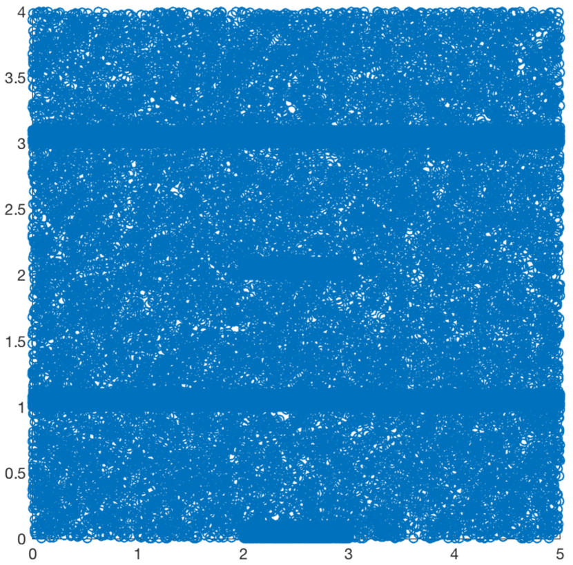
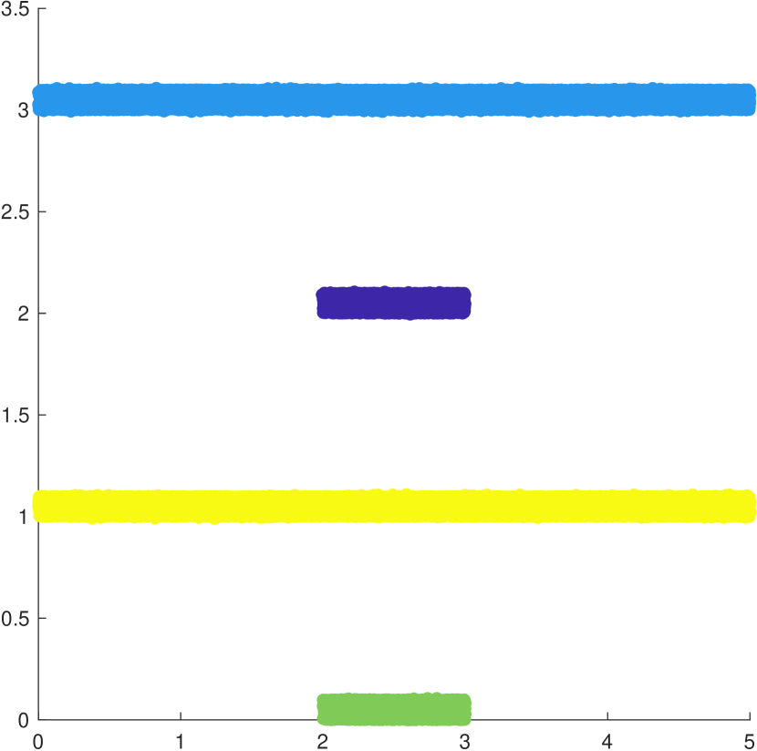
Refer to caption
(a) Four Lines
Refer to caption
(b) LLPD spectral clustering on denoised Four Lines
Refer to caption
(c) Nine Gaussians
Refer to caption
(d) LLPD spectral clustering on denoised Nine Gaussians
Figure 8: Two dimensional synthetic data sets and LLPD spectral clustering results for the denoised data sets. In Figures 8(b) and 8(d), color corresponds to the label returned by LLPD spectral clustering.

Figure 9 illustrates the denoising procedure. Sorted LLPD-nearest neighbor distances are shown in blue, and the denoising threshold θ𝜃\theta (selected by choosing the graph elbow) is shown in red. All plots exhibit an elbow pattern, which is shallow when D/d𝐷𝑑D/d is small (Figure 9(b)) and sharp when D/d𝐷𝑑D/d is large (Figure 9(c); the sharpness is due to the drastic difference in nearest neighbor distances for cluster and noise points).
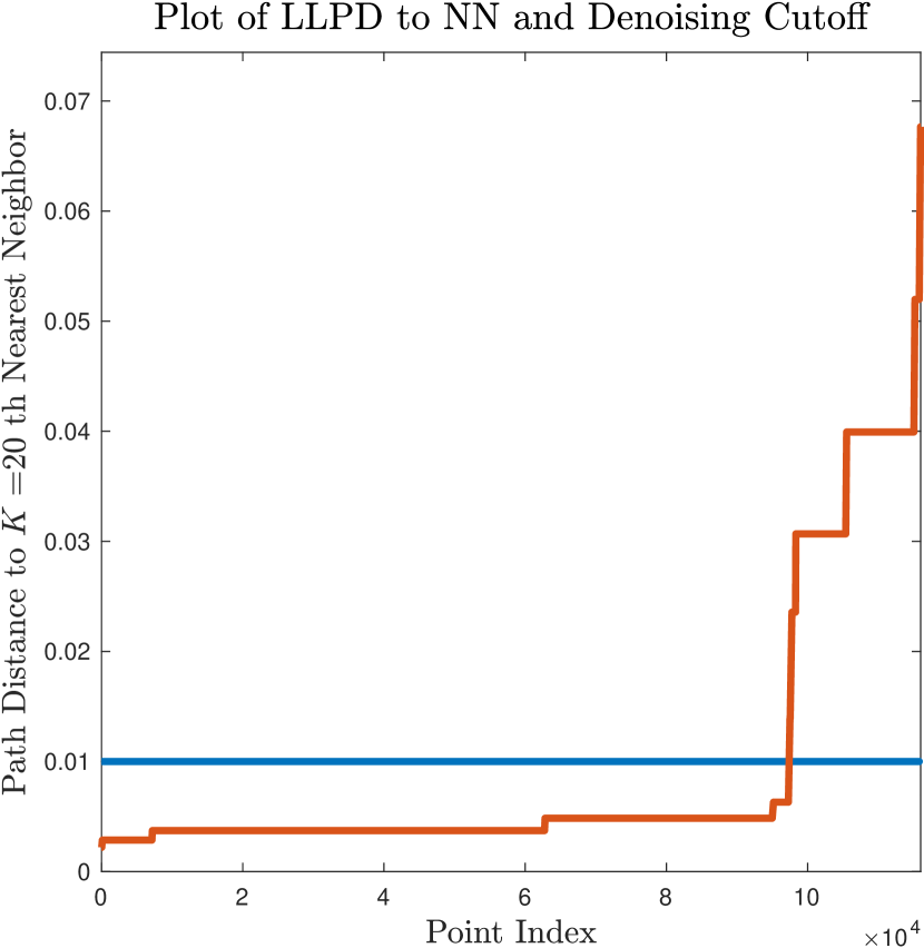
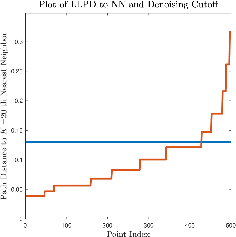
Refer to caption
(a) Four Lines
Refer to caption
(b) Nine Gaussians
Refer to caption
(c) Concentric Spheres
Refer to caption
(d) Parallel Planes
Figure 9: LLPD to knsethsuperscriptsubscript𝑘nseth{k_{\text{nse}}}^{\!\!\!\!\!\text{th}} LLPD-nearest neighbor (blue) and threshold θ𝜃\theta used for denoising the data (red).

Figure 10 shows the multiscale eigenvalue plots for the synthetic data sets. For the four lines data, Euclidean spectral clustering is run with n=1160𝑛1160n=1160 since it is prohibitively slow for n=116000𝑛116000n=116000; however all relevant proportions such as n~/ni~𝑛subscript𝑛𝑖\tilde{n}/n_{i} are the same. LLPD spectral clustering correctly infers K𝐾K for all synthetic data sets; Euclidean spectral clustering fails to correctly infers K𝐾K except for the nine Gaussians example. See Table 2 for all K^^𝐾\hat{K} values and empirical accuracies. Although accuracy is reported on the cluster points only, we remark that labels can be extended to any noise points which survive denoising by considering the label of the closest cluster set, and the empirical accuracies reported in Table 2 remain essentially unchanged.

In addition to learning the number of clusters K𝐾K, the multiscale eigenvalue plots can also be used to infer a good scale σ𝜎\sigma for LLPD spectral clustering as σ^=argmaxσ(λK^+1(σ)λK^(σ)).^𝜎subscriptargmax𝜎subscript𝜆^𝐾1𝜎subscript𝜆^𝐾𝜎\hat{\sigma}=\operatorname*{arg\,max}_{\sigma}\left(\lambda_{\hat{K}+1}(\sigma)-\lambda_{\hat{K}}(\sigma)\right). For the two dimensional examples, the right panel of Figure 8 shows the results of LLPD spectral clustering with K^^𝐾\hat{K}, σ^^𝜎\hat{\sigma} inferred from the maximal eigengap with LLPD. Robustly estimating K𝐾K and σ𝜎\sigma makes LLPD spectral clustering essentially parameter free, and thus highly desirable for the analysis of real data.
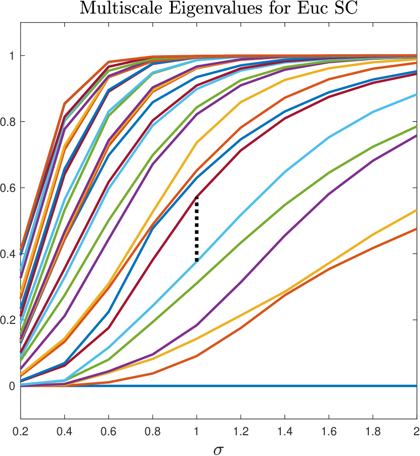
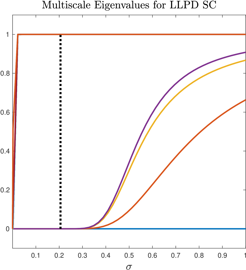
Refer to caption
Refer to caption
(a) Four Lines
Refer to caption
Refer to caption
(b) Nine Gaussians
Refer to caption
Refer to caption
(c) Concentric Spheres
Refer to caption
Refer to caption
(d) Parallel Planes
Figure 10: Multiscale eigenvalues of LSYMsubscript𝐿SYM{L_{\text{SYM}}} for synthetic data sets using Euclidean distance (top) and LLPD (bottom).

7.2 Real Data

Refer to caption
(a) Skins data
Refer to caption
(b) DrivFace Representative Faces
Refer to caption
(c) COIL objects
Refer to caption
(d) COIL 16 objects
Figure 11: Representative objects from (a) Skins, (b) DrivFace, (c) COIL, and (d) COIL 16 data sets.

We apply our method on the following real data sets:

  • Skins This large dataset consists of RGB values corresponding to pixels sampled from two classes: human skin and other222https://archive.ics.uci.edu/ml/datasets/skin+segmentation. The human skin samples are widely sampled with respect to age, gender, and skin color; see Bhatt et al. (2009) for details on the construction of the dataset. This dataset consists of 245057 data points in D=3𝐷3D=3 dimensions, corresponding to the RGB values. Note LLPD was approximated from scales {ts}s=1msuperscriptsubscriptsubscript𝑡𝑠𝑠1𝑚\{t_{s}\}_{s=1}^{m} defined by 10 percentiles, as opposed to the default exponential scaling. See Figure 11(a).

  • DrivFace The DrivFace data set is publicly available333https://archive.ics.uci.edu/ml/datasets/DrivFace from the UCI Machine Learning Repository (Lichman, 2013). This data set consists of 606 80×80808080\times 80 pixel images of the faces of four drivers, 2 male and 2 female. See Figure 11(b)

  • COIL The COIL (Columbia University Image Library) dataset444http://www.cs.columbia.edu/CAVE/software/softlib/coil-20.php consists of images of 20 different objects captured at varying angles (Nene et al., 1996). There are 1440 different data points, each of which is a 32×32323232\times 32 image, thought of as a D=1024𝐷1024D=1024 dimensional point cloud. See Figure 11(c).

  • COIL 16 To ease the problem slightly, we consider a 16 class subset of the full COIL data, shown in Figure 11(d).

  • Pen Digits This dataset555https://archive.ics.uci.edu/ml/datasets/Pen-Based+Recognition+of+Handwritten+Digits consists of 3779 spatially resampled digital signals of hand-written digits in 16 dimensions (Alimoglu and Alpaydin, 1996). We consider a subset consisting of five digits: {0,2,3,4,6}02346\{0,2,3,4,6\}.

  • Landsat The landsat satellite data we consider consists of pixels in 3×3333\times 3 neighborhoods in a multispectral camera with four spectral bands666https://archive.ics.uci.edu/ml/datasets/Statlog+(Landsat+Satellite). This leads to a total ambient dimension of D=36𝐷36D=36. The data considered consists of K=4𝐾4K=4 classes, consisting of pixels of different physical materials: red soil, cotton, damp soil, and soil with vegetable stubble.
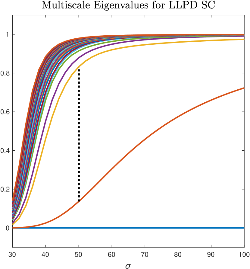
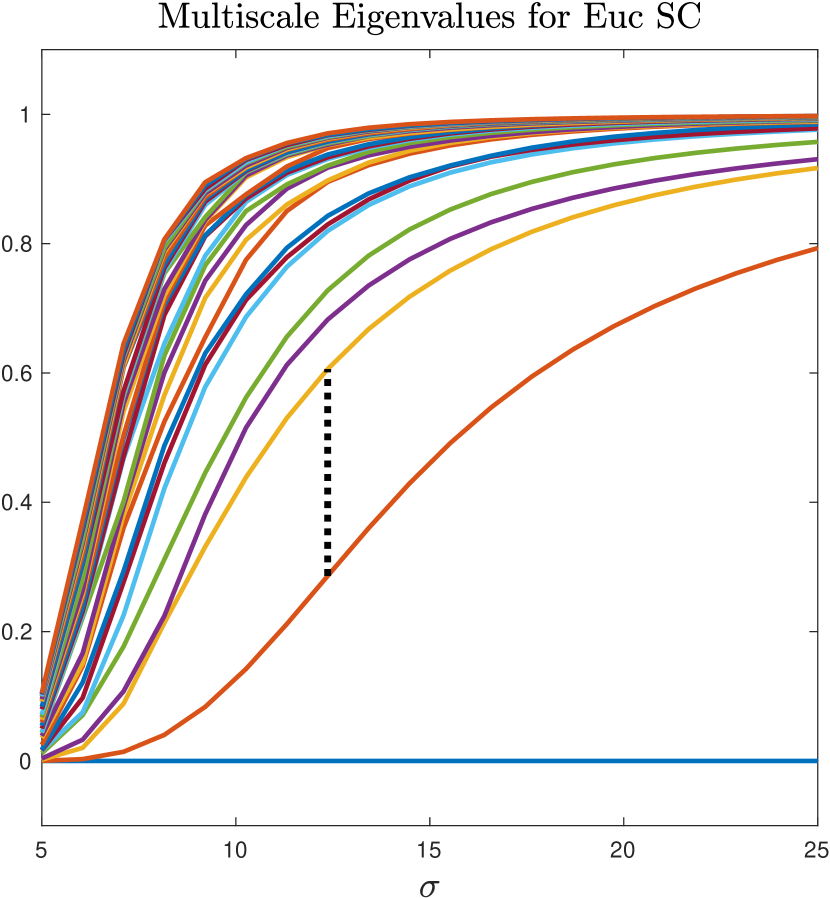
Refer to caption
(a) Skins: LLPD eigenvalues
Refer to caption
Refer to caption
(b) DrivFace
Refer to caption
Refer to caption
(c) COIL 16
Refer to caption
Refer to caption
(d) Pen Digits
Refer to caption
Refer to caption
(e) Landsat
Figure 12: Multiscale eigenvalues of LSYMsubscript𝐿SYM{L_{\text{SYM}}} for real data sets using Euclidean distance (top, (b)-(e), does not appear for (a)) and LLPD (bottom (a)-(e)).

Labeling accuracy results as well as the K^^𝐾\hat{K} values returned by our algorithm are given in Table 2. LLPD spectral clustering correctly estimates K𝐾K for all data sets except the full COIL data set and Landsat. Euclidean spectral clustering fails to correctly detect K𝐾K on all real data sets. Figure 12 shows both the Euclidean and LLPD eigenvalues for Skins, DrivFace, COIL 16, Pen Digits, and Landsat. Euclidean spectral clustering results for Skins are omitted because Euclidean spectral clustering with a dense Laplacian is computationally intractable with such a large sample size.

At least 90%percent9090\% of data points were retained during the denoising procedure with the exception of Skins (88.0%percent88.088.0\% retained) and Landsat (67.2%percent67.267.2\% retained). After denoising, LLPD spectral clustering achieved an overall accuracy exceeding 98.6%percent98.698.6\% on all real data sets except COIL 20 (90.5%percent90.590.5\%). Euclidean spectral clustering performed well on DrivFaces (OA 94.1%percent94.194.1\%) and Pen Digits (OA 98.1%percent98.198.1\%), but poorly on the remaining data sets, where the overall accuracy ranged from 68.9%76.8%percent68.9percent76.868.9\%-76.8\%. K𝐾K-means also performed well on DrivFaces (OA 87.5%percent87.587.5\%) and Pen Digits (OA 97.6%percent97.697.6\%) but poorly on the remaining data sets, where the overall accuracy ranged from 54.7%78.5%percent54.7percent78.554.7\%-78.5\%.

Data Set Accuracy Statistic K𝐾K-means Euclidean SC LLPD SC Four Lines (n=116000,n~=20000,N=97361,D=2,d=1,K=4,ζN=12.0239,θ=.01,σ^=0.2057,δ=.9001formulae-sequence𝑛116000formulae-sequence~𝑛20000formulae-sequence𝑁97361formulae-sequence𝐷2formulae-sequence𝑑1formulae-sequence𝐾4formulae-sequencesubscript𝜁𝑁12.0239formulae-sequence𝜃.01formulae-sequence^𝜎0.2057𝛿.9001n=116000,\tilde{n}=20000,N=97361,D=2,d=1,K=4,\zeta_{N}=12.0239,\theta=.01,\hat{\sigma}=0.2057,\delta=.9001) OA .4951 .6838 1.000 AA .4944 .6995 1.000 κ𝜅\kappa .3275 .5821 1.000 K^^𝐾\hat{K} - 6 4 Nine Gaussians (n=500,n~=0,N=428,D=2,d=2,K=9,ζN=10.7,θ=.13,σ^=0.1000,δ=.1094formulae-sequence𝑛500formulae-sequence~𝑛0formulae-sequence𝑁428formulae-sequence𝐷2formulae-sequence𝑑2formulae-sequence𝐾9formulae-sequencesubscript𝜁𝑁10.7formulae-sequence𝜃.13formulae-sequence^𝜎0.1000𝛿.1094n=500,\tilde{n}=0,N=428,D=2,d=2,K=9,\zeta_{N}=10.7,\theta=.13,\hat{\sigma}=0.1000,\delta=.1094) OA .9930 .9930 .9930 AA .9920 .9920 .9920 κ𝜅\kappa .9921 .9921 .9921 K^^𝐾\hat{K} - 9 9 Concentric Spheres (n=3813,n~=2000,N=1813,D=1000,d=2,K=3,ζN=7.2520,θ=2,σ^=0.1463,δ=.5formulae-sequence𝑛3813formulae-sequence~𝑛2000formulae-sequence𝑁1813formulae-sequence𝐷1000formulae-sequence𝑑2formulae-sequence𝐾3formulae-sequencesubscript𝜁𝑁7.2520formulae-sequence𝜃2formulae-sequence^𝜎0.1463𝛿.5n=3813,\tilde{n}=2000,N=1813,D=1000,d=2,K=3,\zeta_{N}=7.2520,\theta=2,\hat{\sigma}=0.1463,\delta=.5) OA .3464 .3519 .9989 AA .3463 .3438 .9988 κ𝜅\kappa .0094 .0155 .9981 K^^𝐾\hat{K} - 4 3 Parallel Planes
(n=205000,n~=200000,N=5000,D=30,d=10,K=5,ζN=5,θ=.45,σ^=0.0942,δ=.3553formulae-sequence𝑛205000formulae-sequence~𝑛200000formulae-sequence𝑁5000formulae-sequence𝐷30formulae-sequence𝑑10formulae-sequence𝐾5formulae-sequencesubscript𝜁𝑁5formulae-sequence𝜃.45formulae-sequence^𝜎0.0942𝛿.3553n=205000,\tilde{n}=200000,N=5000,D=30,d=10,K=5,\zeta_{N}=5,\theta=.45,\hat{\sigma}=0.0942,\delta=.3553)
OA .5594 .3964 .9990
AA .5594 .3964 .9990 κ𝜅\kappa .4493 .2455 .9987 K^^𝐾\hat{K} - 2 5 Skins (n=245057,N=215694,D=3,K=2,ζN=4.5343,θ=2,σ^=50,δ^=0formulae-sequence𝑛245057formulae-sequence𝑁215694formulae-sequence𝐷3formulae-sequence𝐾2formulae-sequencesubscript𝜁𝑁4.5343formulae-sequence𝜃2formulae-sequence^𝜎50^𝛿0n=245057,N=215694,D=3,K=2,\zeta_{N}=4.5343,\theta=2,\hat{\sigma}=50,\hat{\delta}=0) OA .5473 - .9962 AA .4051 - .9970 κ𝜅\kappa -.1683 - .9890 K^^𝐾\hat{K} - - 2 DrivFaces
(n=612,N=574,D=6400,K=4,ζN=6.4494,θ=10,σ^=4.9474,δ^=9.5976formulae-sequence𝑛612formulae-sequence𝑁574formulae-sequence𝐷6400formulae-sequence𝐾4formulae-sequencesubscript𝜁𝑁6.4494formulae-sequence𝜃10formulae-sequence^𝜎4.9474^𝛿9.5976n=612,N=574,D=6400,K=4,\zeta_{N}=6.4494,\theta=10,\hat{\sigma}=4.9474,\hat{\delta}=9.5976)
OA .8746 .9408 1.000
AA .8882 .9476 1.000 κ𝜅\kappa .9198 .9198 1.000 K^^𝐾\hat{K} - 2 4 COIL 20
(n=1440,N=1351,D=1024,K=20,ζN=27.5714,θ=4.5,σ^=1.9211,δ^=3.3706formulae-sequence𝑛1440formulae-sequence𝑁1351formulae-sequence𝐷1024formulae-sequence𝐾20formulae-sequencesubscript𝜁𝑁27.5714formulae-sequence𝜃4.5formulae-sequence^𝜎1.9211^𝛿3.3706n=1440,N=1351,D=1024,K=20,\zeta_{N}=27.5714,\theta=4.5,\hat{\sigma}=1.9211,\hat{\delta}=3.3706)
OA .6555 .6890 .9055
AA .6290 .6726 .8833 κ𝜅\kappa .6368 .6724 .9004 K^^𝐾\hat{K} - 3 17 COIL 16 (n=1152,N=1088,D=1024,K=16,ζN=22.1837,θ=3.9,σ^=2.3316,δ^=5.4350formulae-sequence𝑛1152formulae-sequence𝑁1088formulae-sequence𝐷1024formulae-sequence𝐾16formulae-sequencesubscript𝜁𝑁22.1837formulae-sequence𝜃3.9formulae-sequence^𝜎2.3316^𝛿5.4350n=1152,N=1088,D=1024,K=16,\zeta_{N}=22.1837,\theta=3.9,\hat{\sigma}=2.3316,\hat{\delta}=5.4350) OA .7500 .7330 1.000 AA .7311 .6782 1.000 κ𝜅\kappa .7330 .6864 1.000 K^^𝐾\hat{K} - 3 16 Pen Digits (n=3779,N=3750,D=16,K=5,ζN=5.2228,θ=60,σ^=16.8421,δ^=11.3137formulae-sequence𝑛3779formulae-sequence𝑁3750formulae-sequence𝐷16formulae-sequence𝐾5formulae-sequencesubscript𝜁𝑁5.2228formulae-sequence𝜃60formulae-sequence^𝜎16.8421^𝛿11.3137n=3779,N=3750,D=16,K=5,\zeta_{N}=5.2228,\theta=60,\hat{\sigma}=16.8421,\hat{\delta}=11.3137) OA .9760 .9813 .9949 AA .9764 .9816 .9949 κ𝜅\kappa .9700 .9767 .9937 K^^𝐾\hat{K} - 6 5 Landsat
(n=1136,N=763,D=36,K=4,ζN=8.4778,θ=32,σ^=51.5789,δ^=28.2489formulae-sequence𝑛1136formulae-sequence𝑁763formulae-sequence𝐷36formulae-sequence𝐾4formulae-sequencesubscript𝜁𝑁8.4778formulae-sequence𝜃32formulae-sequence^𝜎51.5789^𝛿28.2489n=1136,N=763,D=36,K=4,\zeta_{N}=8.4778,\theta=32,\hat{\sigma}=51.5789,\hat{\delta}=28.2489)
OA .7851 .7680 .9869
AA .8619 .8532 .9722 κ𝜅\kappa .6953 .6722 .9802 K^^𝐾\hat{K} - 2 2

Table 2: In all examples, LLPD spectral clustering performs at least as well as K𝐾K-means and Euclidean spectral clustering, and it typically outperforms both. Best results for each method and performance metric are bolded. For each dataset, we include parameters that determine the theoretical results. For both real and synthetic datasets, n𝑛n (the total number of data points), N𝑁N (the number of data points after denoising), D𝐷D (the ambient dimension of the data), K𝐾K (the number of clusters in the data), ζNsubscript𝜁𝑁\zeta_{N} (cluster balance parameter on the denoised data), θ𝜃\theta (LLPD denoising threshold), and σ^^𝜎\hat{\sigma} (learned scaling parameter in LLPD weight matrix) are given. For the synthetic data, n~~𝑛\tilde{n} (number of noise points), d𝑑d (intrinsic dimension of the data), and δ𝛿\delta (minimal Euclidean distance between clusters) are given, since these are known or can be computed exactly. For the real data, δ^^𝛿\hat{\delta} (the minimal Euclidean distanced between clusters, after denoising) is provided. We remark that for the Skins dataset, a very small number of points (which are integer triples in 3superscript3\mathbb{R}^{3}) appear in both classes, so that δ^=0^𝛿0\hat{\delta}=0. Naturally these points are not classified correctly, which leads to a slightly imperfect accuracy for LLPD spectral clustering.

8 Conclusions and Future Directions

This article developed finite sample estimates on the behavior of the LLPD metric, derived theoretical guarantees for spectral clustering with the LLPD, and introduced fast approximate algorithms for computing the LLPD and LLPD spectral clustering. The theoretical guarantees on the eigengap provide mathematical rigor for the heuristic claim that the eigengap determines the number of clusters, and theoretical guarantees on labeling accuracy improve on the state of the art in the LDLN data model. Moreover, the proposed approximation scheme enables efficient LLPD spectral clustering on large, high-dimensional datasets. Our theoretical results are verified numerically, and it is shown that LLPD spectral clustering determines the number of clusters and labels points with high accuracy in many cases where Euclidean spectral clustering fails. In a sense, the method proposed in this article combines two different clustering techniques: density techniques like DBSCAN and single linkage clustering, and spectral clustering. The combination allows for improved robustness and performance guarantees compared to either set of techniques alone.

It is of interest to generalize and improve the results in this article. Our theoretical results involved two components. First, we proved estimates on distances between points under the LLPD metric, under the assumption that data fits the LDLN model. Second, we proved that the weight matrix corresponding to these distances enjoys a structure which guarantees that the eigengap in the normalized graph Laplacian is informative. The first part of this program is generalizable to other distance metrics and data drawn from different distributions. Indeed, one can interpret the LLPD as a minimum over the superscript\ell^{\infty} norm of paths between points. Norms other than the superscript\ell^{\infty} norm may correspond to interesting metrics for data drawn from some class of distributions, for example, the geodesic distance with respect to some metric on a manifold. Moreover, introducing a comparison of tangent-planes into the spectral clustering distance metric has been shown to be effective in the Euclidean setting (Arias-Castro et al., 2017), and allows one to distinguish between intersecting clusters in many cases. Introducing tangent plane comparisons into the LLPD construction would perhaps allow the results in this article to generalize to data drawn from intersecting distributions.

An additional problem not addressed in the present article is the consistency of LLPD spectral clustering. It is of interest to consider the behavior as n𝑛n\rightarrow\infty and determine if LLPD spectral clustering converges in the large sample limit to a continuum partial differential equation. This line of work has been fruitfully developed in recent years for spectral clustering with Euclidean distances (Garcia Trillos et al., 2016; Garcia Trillos and Slepcev, 2016a, b).


Acknowledgments

MM and JMM are grateful for partial support by NSF-IIS-1708553, NSF-DMS-1724979, NSF-CHE-1708353 and AFOSR FA9550-17-1-0280.

A Proofs from Section 4

Proof of Lemma 4.1

Let yS𝑦𝑆y\in S satisfy xy2τsubscriptnorm𝑥𝑦2𝜏\|x-y\|_{2}\leq\tau. Suppose τϵ/4𝜏italic-ϵ4\tau\geq{\epsilon}/{4}. For the upper bound, we have:

D(B(S,τ)Bϵ(x))D(Bϵ(x))=D(B1)ϵDD(B1)ϵd4Dd(τϵ)Dd.superscript𝐷𝐵𝑆𝜏subscript𝐵italic-ϵ𝑥superscript𝐷subscript𝐵italic-ϵ𝑥superscript𝐷subscript𝐵1superscriptitalic-ϵ𝐷superscript𝐷subscript𝐵1superscriptitalic-ϵ𝑑superscript4𝐷𝑑superscript𝜏italic-ϵ𝐷𝑑\mathcal{H}^{D}(B(S,\tau)\cap B_{\epsilon}(x))\leq\mathcal{H}^{D}(B_{\epsilon}(x))=\mathcal{H}^{D}(B_{1})\epsilon^{D}\leq\mathcal{H}^{D}(B_{1})\epsilon^{d}4^{D-d}\left(\tau\wedge\epsilon\right)^{D-d}.

For the lower bound, set z=(1α)x+αy,α=ϵ4τ.formulae-sequence𝑧1𝛼𝑥𝛼𝑦𝛼italic-ϵ4𝜏z=(1-\alpha)x+\alpha y,\ \alpha=\frac{\epsilon}{4\tau}. Then zx2ϵ/4subscriptnorm𝑧𝑥2italic-ϵ4\|z-x\|_{2}\leq{\epsilon}/{4} and zy2τϵ/4subscriptnorm𝑧𝑦2𝜏italic-ϵ4\|z-y\|_{2}\leq\tau-{\epsilon}/{4}, so Bϵ/4(z)B(S,τ)Bϵ(x)subscript𝐵italic-ϵ4𝑧𝐵𝑆𝜏subscript𝐵italic-ϵ𝑥B_{{\epsilon}/{4}}(z)\subset B(S,\tau)\cap B_{\epsilon}(x), and

4DD(B1)ϵd(ϵτ)Dd4DD(B1)ϵD=D(Bϵ/4(z))D(B(S,τ)Bϵ(x)).superscript4𝐷superscript𝐷subscript𝐵1superscriptitalic-ϵ𝑑superscriptitalic-ϵ𝜏𝐷𝑑superscript4𝐷superscript𝐷subscript𝐵1superscriptitalic-ϵ𝐷superscript𝐷subscript𝐵italic-ϵ4𝑧superscript𝐷𝐵𝑆𝜏subscript𝐵italic-ϵ𝑥4^{-D}\mathcal{H}^{D}(B_{1})\epsilon^{d}(\epsilon\wedge\tau)^{D-d}\leq 4^{-D}\mathcal{H}^{D}(B_{1})\epsilon^{D}=\mathcal{H}^{D}(B_{{\epsilon}/{4}}(z))\leq\mathcal{H}^{D}(B(S,\tau)\cap B_{\epsilon}(x)).

This shows that (4.1) holds in the case τϵ/4𝜏italic-ϵ4\tau\geq{\epsilon}/{4}.

Now suppose τ<ϵ/4.𝜏italic-ϵ4\tau<{\epsilon}/{4}. We consider two cases, with the second to be reduced to the first one.

Case 1: x=yS𝑥𝑦𝑆x=y\in S. Let {yi}i=1nsuperscriptsubscriptsubscript𝑦𝑖𝑖1𝑛\{y_{i}\}_{i=1}^{n} be a τ𝜏\tau-packing of SBϵτ(y)𝑆subscript𝐵italic-ϵ𝜏𝑦S\cap B_{\epsilon-\tau}(y), i.e.: SBϵτ(y)i=1nBτ(yi)𝑆subscript𝐵italic-ϵ𝜏𝑦superscriptsubscript𝑖1𝑛subscript𝐵𝜏subscript𝑦𝑖S\cap B_{\epsilon-\tau}(y)\subset\bigcup_{i=1}^{n}B_{\tau}(y_{i}), and yiyj2>τ,ijformulae-sequencesubscriptnormsubscript𝑦𝑖subscript𝑦𝑗2𝜏𝑖𝑗\|y_{i}-y_{j}\|_{2}>\tau,i\neq j. We show this implies that B(S,τ)Bϵ2(y)i=1nB2τ(yi)𝐵𝑆𝜏subscript𝐵italic-ϵ2𝑦superscriptsubscript𝑖1𝑛subscript𝐵2𝜏subscript𝑦𝑖B(S,\tau)\cap B_{\frac{\epsilon}{2}}(y)\subset\bigcup_{i=1}^{n}B_{2\tau}(y_{i}). Indeed, let x0B(S,τ)Bϵ2(y)subscript𝑥0𝐵𝑆𝜏subscript𝐵italic-ϵ2𝑦x_{0}\in B(S,\tau)\cap B_{\frac{\epsilon}{2}}(y). Then there is some xSsuperscript𝑥𝑆x^{*}\in S such that x0x2τsubscriptnormsubscript𝑥0superscript𝑥2𝜏\|x_{0}-x^{*}\|_{2}\leq\tau, and so xy2xx02+x0y2τ+ϵ/2<ϵτsubscriptnormsuperscript𝑥𝑦2subscriptnormsuperscript𝑥subscript𝑥02subscriptnormsubscript𝑥0𝑦2𝜏italic-ϵ2italic-ϵ𝜏\|x^{*}-y\|_{2}\leq\|x^{*}-x_{0}\|_{2}+\|x_{0}-y\|_{2}\leq\tau+{\epsilon}/{2}<\epsilon-\tau (since τ<ϵ/4𝜏italic-ϵ4\tau<{\epsilon}/{4}), and hence xSBϵτ(y)superscript𝑥𝑆subscript𝐵italic-ϵ𝜏𝑦x^{*}\in S\cap B_{\epsilon-\tau}(y). Thus there exists yisuperscriptsubscript𝑦𝑖y_{i}^{*} in the τ𝜏\tau-packing of SBϵτ(y)𝑆subscript𝐵italic-ϵ𝜏𝑦S\cap B_{\epsilon-\tau}(y) such that xBτ(yi)superscript𝑥subscript𝐵𝜏superscriptsubscript𝑦𝑖x^{*}\in B_{\tau}(y_{i}^{*}), so that x0yi2x0x2+xyi22τsubscriptnormsubscript𝑥0superscriptsubscript𝑦𝑖2subscriptnormsubscript𝑥0superscript𝑥2subscriptnormsuperscript𝑥superscriptsubscript𝑦𝑖22𝜏\|x_{0}-y_{i}^{*}\|_{2}\leq\|x_{0}-x^{*}\|_{2}+\|x^{*}-y_{i}^{*}\|_{2}\leq 2\tau, and x0B2τ(yi)subscript𝑥0subscript𝐵2𝜏superscriptsubscript𝑦𝑖x_{0}\in B_{2\tau}(y_{i}^{*}). Hence,

D(B(S,τ)Bϵ2(y))i=1nD(B2τ(yi))=nD(B1)2DτD.superscript𝐷𝐵𝑆𝜏subscript𝐵italic-ϵ2𝑦superscriptsubscript𝑖1𝑛superscript𝐷subscript𝐵2𝜏subscript𝑦𝑖𝑛superscript𝐷subscript𝐵1superscript2𝐷superscript𝜏𝐷\mathcal{H}^{D}(B(S,\tau)\cap B_{\frac{\epsilon}{2}}(y))\leq\sum_{i=1}^{n}\mathcal{H}^{D}(B_{2\tau}(y_{i}))=n\mathcal{H}^{D}(B_{1})2^{D}\tau^{D}. (A.1)

Similarly, it is straight-forward to verify that i=1nBτ2(yi)B(S,τ)Bϵ(y),superscriptsubscript𝑖1𝑛subscript𝐵𝜏2subscript𝑦𝑖𝐵𝑆𝜏subscript𝐵italic-ϵ𝑦\bigcup_{i=1}^{n}B_{\frac{\tau}{2}}(y_{i})\subset B(S,\tau)\cap B_{\epsilon}(y), and since the {Bτ2(yi)}i=1nsuperscriptsubscriptsubscript𝐵𝜏2subscript𝑦𝑖𝑖1𝑛\{B_{\frac{\tau}{2}}(y_{i})\}_{i=1}^{n} are pairwise disjoint, it follows that

nD(B1)2DτD=D(i=1nBτ2(yi))D(B(S,τ)Bϵ(y)).𝑛superscript𝐷subscript𝐵1superscript2𝐷superscript𝜏𝐷superscript𝐷superscriptsubscript𝑖1𝑛subscript𝐵𝜏2subscript𝑦𝑖superscript𝐷𝐵𝑆𝜏subscript𝐵italic-ϵ𝑦n\mathcal{H}^{D}(B_{1})2^{-D}\tau^{D}=\mathcal{H}^{D}\left(\cup_{i=1}^{n}B_{\frac{\tau}{2}}(y_{i})\right)\leq\mathcal{H}^{D}(B(S,\tau)\cap B_{\epsilon}(y)). (A.2)

We now estimate n𝑛n. Indeed, SBϵ2(y)SBϵτ(y)i=1nSBτ(yi),𝑆subscript𝐵italic-ϵ2𝑦𝑆subscript𝐵italic-ϵ𝜏𝑦superscriptsubscript𝑖1𝑛𝑆subscript𝐵𝜏subscript𝑦𝑖S\cap B_{\frac{\epsilon}{2}}(y)\subset S\cap B_{\epsilon-\tau}(y)\subset\bigcup_{i=1}^{n}S\cap B_{\tau}(y_{i}), so that by assumption S𝒮d(κ,ϵ0)𝑆subscript𝒮𝑑𝜅subscriptitalic-ϵ0S\in\mathcal{S}_{d}(\kappa,\epsilon_{0}) and ϵ(0,2ϵ05)(0,ϵ0)italic-ϵ02subscriptitalic-ϵ050subscriptitalic-ϵ0\epsilon\in(0,\frac{2\epsilon_{0}}{5})\subset(0,\epsilon_{0}),

2dϵdκ1d(B1)d(SBϵ2(y))i=1nd(SBτ(yi))κτdnd(B1).superscript2𝑑superscriptitalic-ϵ𝑑superscript𝜅1superscript𝑑subscript𝐵1superscript𝑑𝑆subscript𝐵italic-ϵ2𝑦superscriptsubscript𝑖1𝑛superscript𝑑𝑆subscript𝐵𝜏subscript𝑦𝑖𝜅superscript𝜏𝑑𝑛superscript𝑑subscript𝐵12^{-d}\epsilon^{d}\kappa^{-1}\mathcal{H}^{d}(B_{1})\leq\mathcal{H}^{d}(S\cap B_{\frac{\epsilon}{2}}(y))\leq\sum_{i=1}^{n}\mathcal{H}^{d}(S\cap B_{\tau}(y_{i}))\leq\kappa\tau^{d}n\mathcal{H}^{d}(B_{1}).

It follows that

2d(ϵ/τ)dκ2n.superscript2𝑑superscriptitalic-ϵ𝜏𝑑superscript𝜅2𝑛2^{-d}\left({\epsilon}/{\tau}\right)^{d}\kappa^{-2}\leq n. (A.3)

Similarly, i=1nSBτ2(yi)SBϵ(y)superscriptsubscript𝑖1𝑛𝑆subscript𝐵𝜏2subscript𝑦𝑖𝑆subscript𝐵italic-ϵ𝑦\bigcup_{i=1}^{n}S\cap B_{\frac{\tau}{2}}(y_{i})\subset S\cap B_{\epsilon}(y) yields

nκ1τd2dd(B1)i=1nd(SBτ2(yi))d(SBϵ(y))κϵdd(B1),𝑛superscript𝜅1superscript𝜏𝑑superscript2𝑑superscript𝑑subscript𝐵1superscriptsubscript𝑖1𝑛superscript𝑑𝑆subscript𝐵𝜏2subscript𝑦𝑖superscript𝑑𝑆subscript𝐵italic-ϵ𝑦𝜅superscriptitalic-ϵ𝑑superscript𝑑subscript𝐵1n\kappa^{-1}\tau^{d}2^{-d}\mathcal{H}^{d}(B_{1})\leq\sum_{i=1}^{n}\mathcal{H}^{d}(S\cap B_{\frac{\tau}{2}}(y_{i}))\leq\mathcal{H}^{d}(S\cap B_{\epsilon}(y))\leq\kappa\epsilon^{d}\mathcal{H}^{d}(B_{1}),

so that

n2dκ2(ϵ/τ)d.𝑛superscript2𝑑superscript𝜅2superscriptitalic-ϵ𝜏𝑑n\leq 2^{d}\kappa^{2}\left({\epsilon}/{\tau}\right)^{d}. (A.4)

By combining (A.2) and (A.3), we obtain

D(B1)2(d+D)κ2τD(ϵ/τ)dD(B(S,τ)Bϵ(y))superscript𝐷subscript𝐵1superscript2𝑑𝐷superscript𝜅2superscript𝜏𝐷superscriptitalic-ϵ𝜏𝑑superscript𝐷𝐵𝑆𝜏subscript𝐵italic-ϵ𝑦\displaystyle\mathcal{H}^{D}(B_{1})2^{-(d+D)}\kappa^{-2}\tau^{D}\left({\epsilon}/{\tau}\right)^{d}\leq\mathcal{H}^{D}(B(S,\tau)\cap B_{\epsilon}(y)) (A.5)

and by combining (A.1) and (A.4), we obtain

D(B(S,τ)Bϵ2(y))D(B1)2d+Dκ2τD(ϵ/τ)d,superscript𝐷𝐵𝑆𝜏subscript𝐵italic-ϵ2𝑦superscript𝐷subscript𝐵1superscript2𝑑𝐷superscript𝜅2superscript𝜏𝐷superscriptitalic-ϵ𝜏𝑑\displaystyle\mathcal{H}^{D}(B(S,\tau)\cap B_{\frac{\epsilon}{2}}(y))\leq\mathcal{H}^{D}(B_{1})2^{d+D}\kappa^{2}\tau^{D}\left({\epsilon}/{\tau}\right)^{d}, (A.6)

which are valid for any ϵ<ϵ0,τ<ϵ/4formulae-sequenceitalic-ϵsubscriptitalic-ϵ0𝜏italic-ϵ4\epsilon<\epsilon_{0},\tau<{\epsilon}/{4}. Replacing ϵ/2italic-ϵ2{\epsilon}/{2} and τ𝜏\tau with ϵitalic-ϵ\epsilon and 2τ2𝜏2\tau, respectively, in (A.6), and combining with (A.5), we obtain, for ϵ<ϵ0/2,τ<ϵ/4formulae-sequenceitalic-ϵsubscriptitalic-ϵ02𝜏italic-ϵ4\epsilon<{\epsilon_{0}}/{2},\tau<{\epsilon}/{4},

D(B1)2(d+D)κ2τD(ϵ/τ)dD(B(S,τ)Bϵ(y))D(B1)2d+2Dκ2τD(ϵ/τ)d.superscript𝐷subscript𝐵1superscript2𝑑𝐷superscript𝜅2superscript𝜏𝐷superscriptitalic-ϵ𝜏𝑑superscript𝐷𝐵𝑆𝜏subscript𝐵italic-ϵ𝑦superscript𝐷subscript𝐵1superscript2𝑑2𝐷superscript𝜅2superscript𝜏𝐷superscriptitalic-ϵ𝜏𝑑\mathcal{H}^{D}(B_{1})2^{-(d+D)}\kappa^{-2}\tau^{D}\left({\epsilon}/{\tau}\right)^{d}\leq\mathcal{H}^{D}(B(S,\tau)\cap B_{\epsilon}(y))\leq\mathcal{H}^{D}(B_{1})2^{d+2D}\kappa^{2}\tau^{D}\left({\epsilon}/{\tau}\right)^{d}\,.

Case 2: xS𝑥𝑆x\notin S. Notice that xy2τϵ/4subscriptnorm𝑥𝑦2𝜏italic-ϵ4\|x-y\|_{2}\leq\tau\leq{\epsilon}/{4}, so B3ϵ4(y)Bϵ(x)B5ϵ4(y)subscript𝐵3italic-ϵ4𝑦subscript𝐵italic-ϵ𝑥subscript𝐵5italic-ϵ4𝑦B_{\frac{3\epsilon}{4}}(y)\subset B_{\epsilon}(x)\subset B_{\frac{5\epsilon}{4}}(y). Thus: D(B(S,τ)Bϵ(x))D(B(S,τ)B5ϵ4(y))D(B1)22D+2dκ2τD(ϵ/τ)d,superscript𝐷𝐵𝑆𝜏subscript𝐵italic-ϵ𝑥superscript𝐷𝐵𝑆𝜏subscript𝐵5italic-ϵ4𝑦superscript𝐷subscript𝐵1superscript22𝐷2𝑑superscript𝜅2superscript𝜏𝐷superscriptitalic-ϵ𝜏𝑑\mathcal{H}^{D}(B(S,\tau)\cap B_{\epsilon}(x))\leq\mathcal{H}^{D}(B(S,\tau)\cap B_{\frac{5\epsilon}{4}}(y))\leq\mathcal{H}^{D}(B_{1})2^{2D+2d}\kappa^{2}\tau^{D}\left({\epsilon}/{\tau}\right)^{d}, so as long as ϵ<2ϵ05italic-ϵ2subscriptitalic-ϵ05\epsilon<\frac{2\epsilon_{0}}{5} we have

D(B(S,τ)Bϵ(x))superscript𝐷𝐵𝑆𝜏subscript𝐵italic-ϵ𝑥\displaystyle\mathcal{H}^{D}(B(S,\tau)\cap B_{\epsilon}(x)) D(B(S,3τ/4)B3ϵ/4(y))D(B1)2(2D+d)κ2τD(ϵ/τ)d.absentsuperscript𝐷𝐵𝑆3𝜏4subscript𝐵3italic-ϵ4𝑦superscript𝐷subscript𝐵1superscript22𝐷𝑑superscript𝜅2superscript𝜏𝐷superscriptitalic-ϵ𝜏𝑑\displaystyle\geq\mathcal{H}^{D}(B(S,3\tau/4)\cap B_{{3\epsilon}/{4}}(y))\geq\mathcal{H}^{D}(B_{1})2^{-(2D+d)}\kappa^{-2}\tau^{D}\left({\epsilon}/{\tau}\right)^{d}.

We thus obtain the statement in Lemma 4.1.

Proof of Theorem 4.2

Cover B(S,τ)𝐵𝑆𝜏B(S,\tau) with an ϵ/4italic-ϵ4{\epsilon}/{4}-packing {yi}i=1Nsuperscriptsubscriptsubscript𝑦𝑖𝑖1𝑁\{y_{i}\}_{i=1}^{N}, such that B(S,τ)i=1NBϵ/4(yi)𝐵𝑆𝜏superscriptsubscript𝑖1𝑁subscript𝐵italic-ϵ4subscript𝑦𝑖B(S,\tau)\subset\bigcup_{i=1}^{N}B_{{\epsilon}/{4}}(y_{i}), and yiyj2>ϵ/4,ijformulae-sequencesubscriptnormsubscript𝑦𝑖subscript𝑦𝑗2italic-ϵ4for-all𝑖𝑗\|y_{i}-y_{j}\|_{2}>{\epsilon}/{4},\forall i\neq j. {Bϵ/8(yi)}i=1Nsuperscriptsubscriptsubscript𝐵italic-ϵ8subscript𝑦𝑖𝑖1𝑁\{B_{{\epsilon}/{8}}(y_{i})\}_{i=1}^{N} are thus pairwise disjoint, so that i=1ND(Bϵ/8(yi)B(S,τ))D(B(S,τ)).superscriptsubscript𝑖1𝑁superscript𝐷subscript𝐵italic-ϵ8subscript𝑦𝑖𝐵𝑆𝜏superscript𝐷𝐵𝑆𝜏\sum_{i=1}^{N}\mathcal{H}^{D}(B_{{\epsilon}/{8}}(y_{i})\cap B(S,\tau))\leq\mathcal{H}^{D}(B(S,\tau)). By Lemma 4.1, we may bound C1(ϵ/8)d(ϵ/8τ)DdD(Bϵ/8(yi)B(S,τ)),subscript𝐶1superscriptitalic-ϵ8𝑑superscriptitalic-ϵ8𝜏𝐷𝑑superscript𝐷subscript𝐵italic-ϵ8subscript𝑦𝑖𝐵𝑆𝜏C_{1}\left({\epsilon}/{8}\right)^{d}\left({\epsilon}/{8}\wedge\tau\right)^{D-d}\leq\mathcal{H}^{D}(B_{{\epsilon}/{8}}(y_{i})\cap B(S,\tau)), where C1=κ22(2D+d)D(B1).subscript𝐶1superscript𝜅2superscript22𝐷𝑑superscript𝐷subscript𝐵1C_{1}=\kappa^{-2}2^{-(2D+d)}\mathcal{H}^{D}(B_{1}). Hence, NC1(ϵ/8)d(ϵ/8τ)DdD(B(S,τ)),𝑁subscript𝐶1superscriptitalic-ϵ8𝑑superscriptitalic-ϵ8𝜏𝐷𝑑superscript𝐷𝐵𝑆𝜏NC_{1}\left({\epsilon}/{8}\right)^{d}\left({\epsilon}/{8}\wedge\tau\right)^{D-d}\leq\mathcal{H}^{D}(B(S,\tau)), so that

NCD(B(S,τ))(ϵ/8)d(ϵ/8τ)(Dd),C=κ222D+d(D(B1))1.formulae-sequence𝑁𝐶superscript𝐷𝐵𝑆𝜏superscriptitalic-ϵ8𝑑superscriptitalic-ϵ8𝜏𝐷𝑑𝐶superscript𝜅2superscript22𝐷𝑑superscriptsuperscript𝐷subscript𝐵11\displaystyle N\leq C\mathcal{H}^{D}(B(S,\tau))\left({\epsilon}/{8}\right)^{-d}\left({\epsilon}/{8}\wedge\tau\right)^{-(D-d)},\ C=\kappa^{2}2^{2D+d}(\mathcal{H}^{D}(B_{1}))^{-1}.

So, CD(B(S,τ))(ϵ/8)d(ϵ/8τ)(Dd)𝐶superscript𝐷𝐵𝑆𝜏superscriptitalic-ϵ8𝑑superscriptitalic-ϵ8𝜏𝐷𝑑C\mathcal{H}^{D}(B(S,\tau))\left({\epsilon}/{8}\right)^{-d}\left({\epsilon}/{8}\wedge\tau\right)^{-(D-d)} balls of radius ϵ/4italic-ϵ4{\epsilon}/{4} are needed to cover B(S,τ)𝐵𝑆𝜏B(S,\tau). We now determine how many samples n𝑛n must be taken so that each ball contains at least one sample with probability exceeding 1t1𝑡1-t. If this occurs, then each pair of points is connected by a path with all edges of length at most ϵitalic-ϵ\epsilon. Notice that the distribution of the number of points ωisubscript𝜔𝑖\omega_{i} in the set Bϵ/4(yi)B(S,τ)subscript𝐵italic-ϵ4subscript𝑦𝑖𝐵𝑆𝜏B_{{\epsilon}/{4}}(y_{i})\cap B(S,\tau) is ωiBin(n,pi)similar-tosubscript𝜔𝑖Bin𝑛subscript𝑝𝑖\omega_{i}\sim\operatorname*{\text{Bin}}(n,p_{i}), where

pi=D(B(S,τ)Bϵ/4(yi))D(B(S,τ))C1(ϵ/4)d(ϵ/4τ)DdD(B(S,τ)):=p.subscript𝑝𝑖superscript𝐷𝐵𝑆𝜏subscript𝐵italic-ϵ4subscript𝑦𝑖superscript𝐷𝐵𝑆𝜏superscript𝐶1superscriptitalic-ϵ4𝑑superscriptitalic-ϵ4𝜏𝐷𝑑superscript𝐷𝐵𝑆𝜏assign𝑝\displaystyle p_{i}=\frac{\mathcal{H}^{D}(B(S,\tau)\cap B_{{\epsilon}/{4}}(y_{i}))}{\mathcal{H}^{D}(B(S,\tau))}\geq\frac{C^{-1}\left({\epsilon}/{4}\right)^{d}\left({\epsilon}/{4}\wedge\tau\right)^{D-d}}{\mathcal{H}^{D}(B(S,\tau))}:=p.

Since (i:ωi=0)N(1p)nNepnt\mathbb{P}(\exists i:\omega_{i}=0)\leq N(1-p)^{n}\leq Ne^{-pn}\leq t as long as n1/plogN/t𝑛1𝑝𝑁𝑡n\geq 1/p\log N/t, it suffices for n𝑛n to satisfy nCD(B(S,τ))(ϵ/4)d(τϵ/4)DdlogCD(B(S,τ))(ϵ/8)d(τϵ/8)Ddt𝑛𝐶superscript𝐷𝐵𝑆𝜏superscriptitalic-ϵ4𝑑superscript𝜏italic-ϵ4𝐷𝑑𝐶superscript𝐷𝐵𝑆𝜏superscriptitalic-ϵ8𝑑superscript𝜏italic-ϵ8𝐷𝑑𝑡n\geq\frac{C\mathcal{H}^{D}(B(S,\tau))}{\left({\epsilon}/{4}\right)^{d}(\tau\wedge{\epsilon}/{4})^{D-d}}\log\frac{C\mathcal{H}^{D}(B(S,\tau))}{\left({\epsilon}/{8}\right)^{d}(\tau\wedge{\epsilon}/{8})^{D-d}t}.

Proof of Corollary 4.3

For a fixed l𝑙l, choose a τ𝜏\tau packing of Slsubscript𝑆𝑙S_{l}, i.e. let y1,,ymSlsubscript𝑦1subscript𝑦𝑚subscript𝑆𝑙y_{1},\ldots,y_{m}\in S_{l} such that SliBτ(yi)subscript𝑆𝑙subscript𝑖subscript𝐵𝜏subscript𝑦𝑖S_{l}\subset\cup_{i}B_{\tau}(y_{i}) and yiyj2>τsubscriptnormsubscript𝑦𝑖subscript𝑦𝑗2𝜏\|y_{i}-y_{j}\|_{2}>\tau for ij𝑖𝑗i\neq j. Then B(Sl,τ)B2τ(yi)𝐵subscript𝑆𝑙𝜏subscript𝐵2𝜏subscript𝑦𝑖B(S_{l},\tau)\subset B_{2\tau}(y_{i}). Now we control the size of m𝑚m. Since the Bτ2(yi)subscript𝐵𝜏2subscript𝑦𝑖B_{\frac{\tau}{2}}(y_{i}) are disjoint and SlS(κ,ϵ0)subscript𝑆𝑙𝑆𝜅subscriptitalic-ϵ0S_{l}\in S(\kappa,\epsilon_{0}), d(Sl)i=1md(SlBτ2(yi))mκ1d(B1)(τ2)dsuperscript𝑑subscript𝑆𝑙superscriptsubscript𝑖1𝑚superscript𝑑subscript𝑆𝑙subscript𝐵𝜏2subscript𝑦𝑖𝑚superscript𝜅1superscript𝑑subscript𝐵1superscript𝜏2𝑑\mathcal{H}^{d}(S_{l})\geq\sum_{i=1}^{m}\mathcal{H}^{d}(S_{l}\cap B_{\frac{\tau}{2}}(y_{i}))\geq m\kappa^{-1}\mathcal{H}^{d}(B_{1})\left(\frac{\tau}{2}\right)^{d}, so that mκd(Sl)d(B1)(τ2)d𝑚𝜅superscript𝑑subscript𝑆𝑙superscript𝑑subscript𝐵1superscript𝜏2𝑑m\leq\kappa\frac{\mathcal{H}^{d}(S_{l})}{\mathcal{H}^{d}(B_{1})}\left(\frac{\tau}{2}\right)^{-d}. Furthermore, since 25ϵ0>2τ25subscriptitalic-ϵ02𝜏\frac{2}{5}\epsilon_{0}>2\tau we have by Lemma 4.1:

D(B(Sl,τ))D(B1)superscript𝐷𝐵subscript𝑆𝑙𝜏superscript𝐷subscript𝐵1\displaystyle\frac{\mathcal{H}^{D}(B(S_{l},\tau))}{\mathcal{H}^{D}(B_{1})} i=1mD(B(Sl,τ)B2τ(yi))D(B1)mκ22(2D+2d)(2τ)dτDdκ32(2D+4d)d(Sl)d(B1)τDd.absentsuperscriptsubscript𝑖1𝑚superscript𝐷𝐵subscript𝑆𝑙𝜏subscript𝐵2𝜏subscript𝑦𝑖superscript𝐷subscript𝐵1𝑚superscript𝜅2superscript22𝐷2𝑑superscript2𝜏𝑑superscript𝜏𝐷𝑑superscript𝜅3superscript22𝐷4𝑑superscript𝑑subscript𝑆𝑙superscript𝑑subscript𝐵1superscript𝜏𝐷𝑑\displaystyle\leq\sum_{i=1}^{m}\frac{\mathcal{H}^{D}(B(S_{l},\tau)\cap B_{2\tau}(y_{i}))}{\mathcal{H}^{D}(B_{1})}\leq m\kappa^{2}2^{(2D+2d)}\left(2\tau\right)^{d}\tau^{D-d}\leq\kappa^{3}2^{(2D+4d)}\frac{\mathcal{H}^{d}(S_{l})}{\mathcal{H}^{d}(B_{1})}\tau^{D-d}.

Combining the above with (4.2) implies

nlCD(B(Sl,τ))(ϵ/4)dτDdD(B1)logCD(B(Sl,τ))(ϵ/8)dτDdD(B1)tsubscript𝑛𝑙𝐶superscript𝐷𝐵subscript𝑆𝑙𝜏superscriptitalic-ϵ4𝑑superscript𝜏𝐷𝑑superscript𝐷subscript𝐵1𝐶superscript𝐷𝐵subscript𝑆𝑙𝜏superscriptitalic-ϵ8𝑑superscript𝜏𝐷𝑑superscript𝐷subscript𝐵1𝑡n_{l}\geq\frac{C\mathcal{H}^{D}(B(S_{l},\tau))}{\left({\epsilon}/{4}\right)^{d}\tau^{D-d}\mathcal{H}^{D}(B_{1})}\log\frac{C\mathcal{H}^{D}(B(S_{l},\tau))}{\left({\epsilon}/{8}\right)^{d}\tau^{D-d}\mathcal{H}^{D}(B_{1})t}

for C=κ222D+d𝐶superscript𝜅2superscript22𝐷𝑑C=\kappa^{2}2^{2D+d}. Thus by Theorem 4.2, (maxxyXlρ(x,y)<ϵ)1tK.subscript𝑥𝑦subscript𝑋𝑙subscript𝜌𝑥𝑦italic-ϵ1𝑡𝐾\mathbb{P}(\max_{x\neq y\in X_{l}}\rho_{\ell\ell}(x,y)<\epsilon)\geq 1-\frac{t}{K}. Repeating the above argument for each Slsubscript𝑆𝑙S_{l} and letting Elsubscript𝐸𝑙E_{l} denote the event that maxxyXlρ(x,y)ϵsubscript𝑥𝑦subscript𝑋𝑙subscript𝜌𝑥𝑦italic-ϵ\max_{x\neq y\in X_{l}}\rho_{\ell\ell}(x,y)\geq\epsilon, we obtain (ϵinϵ)=(max1lKmaxxyXlρ(x,y)ϵ)=(lEl)l(El)K(tK)=t.subscriptitalic-ϵinitalic-ϵsubscript1𝑙𝐾subscript𝑥𝑦subscript𝑋𝑙subscript𝜌𝑥𝑦italic-ϵsubscript𝑙subscript𝐸𝑙subscript𝑙subscript𝐸𝑙𝐾𝑡𝐾𝑡\mathbb{P}(\epsilon_{\mathrm{in}}\geq\epsilon)=\mathbb{P}(\max_{1\leq l\leq K}\max_{x\neq y\in X_{l}}\rho_{\ell\ell}(x,y)\geq\epsilon)=\mathbb{P}(\cup_{l}E_{l})\leq\sum_{l}\mathbb{P}(E_{l})\leq K(\frac{t}{K})=t.

Proof of Theorem 4.9

Re-writing the inequality assumed in the theorem, we are guaranteed that

C(maxl=1,,K4dκ524D+5dd(Sl)nld(B1)log(2dnl2Kt))1d<((t2)1knse((knse+1)n~)knse+1knseD(X~)D(B1))1D.𝐶superscriptsubscript𝑙1𝐾superscript4𝑑superscript𝜅5superscript24𝐷5𝑑superscript𝑑subscript𝑆𝑙subscript𝑛𝑙superscript𝑑subscript𝐵1superscript2𝑑subscript𝑛𝑙2𝐾𝑡1𝑑superscriptsuperscript𝑡21subscript𝑘nsesuperscriptsubscript𝑘nse1~𝑛subscript𝑘nse1subscript𝑘nsesuperscript𝐷~𝑋superscript𝐷subscript𝐵11𝐷C\left(\max_{l=1,\ldots,K}\frac{4^{d}\kappa^{5}2^{4D+5d}\mathcal{H}^{d}(S_{l})}{n_{l}\mathcal{H}^{d}(B_{1})}\log\left(2^{d}n_{l}\frac{2K}{t}\right)\right)^{\frac{1}{d}}<\left(\frac{\left(\frac{t}{2}\right)^{\frac{1}{{k_{\text{nse}}}}}}{(({k_{\text{nse}}}+1)\tilde{n})^{\frac{{k_{\text{nse}}}+1}{{k_{\text{nse}}}}}}\frac{\mathcal{H}^{D}(\tilde{X})}{\mathcal{H}^{D}(B_{1})}\right)^{\frac{1}{D}}.

Let Cϵ1𝐶subscriptsuperscriptitalic-ϵ1C\epsilon^{*}_{1} denote the left hand side of the above inequality and ϵ2subscriptsuperscriptitalic-ϵ2\epsilon^{*}_{2} the right hand side. Then for all 1lK1𝑙𝐾1\leq l\leq K, nlκ524D+5dd(Sl)(ϵ1/4)dd(B1)(log(2dnl2Kt))subscript𝑛𝑙superscript𝜅5superscript24𝐷5𝑑superscript𝑑subscript𝑆𝑙superscriptsubscriptsuperscriptitalic-ϵ14𝑑superscript𝑑subscript𝐵1superscript2𝑑subscript𝑛𝑙2𝐾𝑡n_{l}\geq\frac{\kappa^{5}2^{4D+5d}\mathcal{H}^{d}(S_{l})}{\left({\epsilon^{*}_{1}}/{4}\right)^{d}\mathcal{H}^{d}(B_{1})}\left(\log\left(2^{d}n_{l}\frac{2K}{t}\right)\right), and since log(2dnl2Kt)1superscript2𝑑subscript𝑛𝑙2𝐾𝑡1\log\left(2^{d}n_{l}\frac{2K}{t}\right)\geq 1, clearly nlκ524D+5dd(Sl)(ϵ1/4)dd(B1)subscript𝑛𝑙superscript𝜅5superscript24𝐷5𝑑superscript𝑑subscript𝑆𝑙superscriptsubscriptsuperscriptitalic-ϵ14𝑑superscript𝑑subscript𝐵1n_{l}\geq\frac{\kappa^{5}2^{4D+5d}\mathcal{H}^{d}(S_{l})}{\left({\epsilon^{*}_{1}}/{4}\right)^{d}\mathcal{H}^{d}(B_{1})}, and we obtain nl(κ524D+5dd(Sl)(ϵ1/4)dd(B1)log(κ524D+5dd(Sl)(ϵ1/8)dd(B1)2Kt))subscript𝑛𝑙superscript𝜅5superscript24𝐷5𝑑superscript𝑑subscript𝑆𝑙superscriptsubscriptsuperscriptitalic-ϵ14𝑑superscript𝑑subscript𝐵1superscript𝜅5superscript24𝐷5𝑑superscript𝑑subscript𝑆𝑙superscriptsubscriptsuperscriptitalic-ϵ18𝑑superscript𝑑subscript𝐵12𝐾𝑡n_{l}\geq\left(\frac{\kappa^{5}2^{4D+5d}\mathcal{H}^{d}(S_{l})}{\left({\epsilon^{*}_{1}}/{4}\right)^{d}\mathcal{H}^{d}(B_{1})}\log\left(\frac{\kappa^{5}2^{4D+5d}\mathcal{H}^{d}(S_{l})}{\left({\epsilon^{*}_{1}}/{8}\right)^{d}\mathcal{H}^{d}(B_{1})}\frac{2K}{t}\right)\right). Since τ<ϵ18ϵ05𝜏subscriptsuperscriptitalic-ϵ18subscriptitalic-ϵ05\tau<\frac{\epsilon^{*}_{1}}{8}\wedge\frac{\epsilon_{0}}{5} by assumption, Corollary 4.3 yields (ϵin<ϵ1)1t2.subscriptitalic-ϵinsubscriptsuperscriptitalic-ϵ11𝑡2\mathbb{P}\left(\epsilon_{\mathrm{in}}<\epsilon^{*}_{1}\right)\geq 1-\frac{t}{2}. Also by Theorem 4.7, (ϵnse>ϵ2)1t2.subscriptitalic-ϵnsesubscriptsuperscriptitalic-ϵ21𝑡2\mathbb{P}(\epsilon_{\mathrm{nse}}>\epsilon^{*}_{2})\geq 1-\frac{t}{2}. Since we are assuming Cϵ1<ϵ2𝐶subscriptsuperscriptitalic-ϵ1subscriptsuperscriptitalic-ϵ2C\epsilon^{*}_{1}<\epsilon^{*}_{2}, (Cϵin<ϵnse)((ϵin<ϵ1)(ϵnse>ϵ2))1t𝐶subscriptitalic-ϵinsubscriptitalic-ϵnsesubscriptitalic-ϵinsubscriptsuperscriptitalic-ϵ1subscriptitalic-ϵnsesubscriptsuperscriptitalic-ϵ21𝑡\mathbb{P}(C\epsilon_{\mathrm{in}}<\epsilon_{\mathrm{nse}})\geq\mathbb{P}((\epsilon_{\mathrm{in}}<\epsilon^{*}_{1})\cap(\epsilon_{\mathrm{nse}}>\epsilon^{*}_{2}))\geq 1-t.

B Proof of Theorem 5.2

Let nl=|Al|subscript𝑛𝑙subscript𝐴𝑙n_{l}=|A_{l}| and ml=|Cl|subscript𝑚𝑙subscript𝐶𝑙m_{l}=|C_{l}| denote the cardinality of the sets in Assumption 1, and let η1:=1fσ(ϵin),ηθ:=1fσ(θ),η2:=fσ(ϵnse).formulae-sequenceassignsubscript𝜂11subscript𝑓𝜎subscriptitalic-ϵinformulae-sequenceassignsubscript𝜂𝜃1subscript𝑓𝜎𝜃assignsubscript𝜂2subscript𝑓𝜎subscriptitalic-ϵnse\eta_{1}:=1-f_{\sigma}(\epsilon_{\mathrm{in}}),\eta_{\theta}:=1-f_{\sigma}(\theta),\eta_{2}:=f_{\sigma}(\epsilon_{\mathrm{nse}}).

B.1 Bounding Entries of Weight Matrix W𝑊W and Degrees

The following Lemma guarantees that the weight matrix will have a convenient structure.

Lemma B.1

For 1lK1𝑙𝐾1\leq l\leq K, let Al,Cl,A~lsubscript𝐴𝑙subscript𝐶𝑙subscript~𝐴𝑙A_{l},C_{l},\tilde{A}_{l} be as in Assumption 1. Then:

  1. 1.

    For each fixed xilClsuperscriptsubscript𝑥𝑖𝑙subscript𝐶𝑙x_{i}^{l}\in C_{l}, xilsuperscriptsubscript𝑥𝑖𝑙x_{i}^{l} is equidistant from all points in Alsubscript𝐴𝑙A_{l}; more precisely:

    ρ(xil,xjl)=minxlAlρ(xil,xl)=:ρil,xilCl,xjlAl,1lK.\rho(x^{l}_{i},x^{l}_{j})=\min_{x^{l}\in A_{l}}\rho(x^{l}_{i},x^{l})=:\rho^{l}_{i},\qquad\forall x^{l}_{i}\in C_{l},x^{l}_{j}\in A_{l},1\leq l\leq K.
  2. 2.

    The distance between any point in A~lsubscript~𝐴𝑙\tilde{A}_{l} and A~ssubscript~𝐴𝑠\tilde{A}_{s} is constant for ls𝑙𝑠l\neq s, that is:

    ρ(xil,xjs)=minxlA~l,xsA~sρ(xl,xs)=:ρl,sxilA~l,xjsA~s,1lsK.\rho(x^{l}_{i},x^{s}_{j})=\min_{x^{l}\in\tilde{A}_{l},x^{s}\in\tilde{A}_{s}}\rho(x^{l},x^{s})=:\rho^{l,s}\qquad\forall x^{l}_{i}\in\tilde{A}_{l},x^{s}_{j}\in\tilde{A}_{s},1\leq l\neq s\leq K.

Proof  To prove (1), let xilClsubscriptsuperscript𝑥𝑙𝑖subscript𝐶𝑙x^{l}_{i}\in C_{l} and xjlAlsubscriptsuperscript𝑥𝑙𝑗subscript𝐴𝑙x^{l}_{j}\in A_{l}. Since ρilsubscriptsuperscript𝜌𝑙𝑖\rho^{l}_{i} is the minimum distance between xilsubscriptsuperscript𝑥𝑙𝑖x^{l}_{i} and a point in Alsubscript𝐴𝑙A_{l}, clearly ρ(xil,xjl)ρil𝜌subscriptsuperscript𝑥𝑙𝑖subscriptsuperscript𝑥𝑙𝑗subscriptsuperscript𝜌𝑙𝑖\rho(x^{l}_{i},x^{l}_{j})\geq\rho^{l}_{i}. Let xlsubscriptsuperscript𝑥𝑙x^{l}_{*} denote the point in Alsubscript𝐴𝑙A_{l} such that ρil=ρ(xil,xl)subscriptsuperscript𝜌𝑙𝑖𝜌subscriptsuperscript𝑥𝑙𝑖subscriptsuperscript𝑥𝑙\rho^{l}_{i}=\rho(x^{l}_{i},x^{l}_{*}). Then ρ(xil,xjl)ρ(xil,xl)ρ(xl,xjl)ρ(xil,xl)ϵin=ρilϵin=ρil.𝜌subscriptsuperscript𝑥𝑙𝑖subscriptsuperscript𝑥𝑙𝑗𝜌subscriptsuperscript𝑥𝑙𝑖subscriptsuperscript𝑥𝑙𝜌subscriptsuperscript𝑥𝑙subscriptsuperscript𝑥𝑙𝑗𝜌subscriptsuperscript𝑥𝑙𝑖subscriptsuperscript𝑥𝑙subscriptitalic-ϵinsubscriptsuperscript𝜌𝑙𝑖subscriptitalic-ϵinsubscriptsuperscript𝜌𝑙𝑖\rho(x^{l}_{i},x^{l}_{j})\leq\rho(x^{l}_{i},x^{l}_{*})\vee\rho(x^{l}_{*},x^{l}_{j})\leq\rho(x^{l}_{i},x^{l}_{*})\vee\epsilon_{\mathrm{in}}=\rho^{l}_{i}\vee\epsilon_{\mathrm{in}}=\rho^{l}_{i}. Thus ρ(xil,xjl)=ρil𝜌subscriptsuperscript𝑥𝑙𝑖subscriptsuperscript𝑥𝑙𝑗subscriptsuperscript𝜌𝑙𝑖\rho(x^{l}_{i},x^{l}_{j})=\rho^{l}_{i}.

To prove (2), let xilA~lsubscriptsuperscript𝑥𝑙𝑖subscript~𝐴𝑙x^{l}_{i}\in\tilde{A}_{l} and xjsA~ssubscriptsuperscript𝑥𝑠𝑗subscript~𝐴𝑠x^{s}_{j}\in\tilde{A}_{s} for ls𝑙𝑠l\neq s. Clearly, ρ(xil,xjs)ρl,s𝜌subscriptsuperscript𝑥𝑙𝑖subscriptsuperscript𝑥𝑠𝑗superscript𝜌𝑙𝑠\rho(x^{l}_{i},x^{s}_{j})\geq\rho^{l,s}. Now let xlA~l,xsA~sformulae-sequencesubscriptsuperscript𝑥𝑙subscript~𝐴𝑙subscriptsuperscript𝑥𝑠subscript~𝐴𝑠x^{l}_{*}\in\tilde{A}_{l},x^{s}_{*}\in\tilde{A}_{s} be the points that achieve the minimum, i.e. ρl,s=ρ(xl,xs)superscript𝜌𝑙𝑠𝜌subscriptsuperscript𝑥𝑙subscriptsuperscript𝑥𝑠\rho^{l,s}=\rho(x^{l}_{*},x^{s}_{*}). Note that ρ(xil,xl)θ𝜌subscriptsuperscript𝑥𝑙𝑖subscriptsuperscript𝑥𝑙𝜃\rho(x^{l}_{i},x^{l}_{*})\leq\theta and similarly for ρ(xjs,xs)𝜌subscriptsuperscript𝑥𝑠𝑗subscriptsuperscript𝑥𝑠\rho(x^{s}_{j},x^{s}_{*}) (if xil,xlsubscriptsuperscript𝑥𝑙𝑖subscriptsuperscript𝑥𝑙x^{l}_{i},x^{l}_{*} are both in Clsubscript𝐶𝑙C_{l}, pick any point zAl𝑧subscript𝐴𝑙z\in A_{l} to obtain ρ(xil,xl)ρ(xil,z)ρ(z,xl)θ𝜌subscriptsuperscript𝑥𝑙𝑖subscriptsuperscript𝑥𝑙𝜌subscriptsuperscript𝑥𝑙𝑖𝑧𝜌𝑧subscriptsuperscript𝑥𝑙𝜃\rho(x^{l}_{i},x^{l}_{*})\leq\rho(x^{l}_{i},z)\vee\rho(z,x^{l}_{*})\leq\theta). Thus:

ρ(xil,xjs)𝜌subscriptsuperscript𝑥𝑙𝑖subscriptsuperscript𝑥𝑠𝑗\displaystyle\rho(x^{l}_{i},x^{s}_{j}) ρ(xil,xl)ρ(xl,xs)ρ(xs,xjs)θρl,sθ=ρl,s,absent𝜌subscriptsuperscript𝑥𝑙𝑖subscriptsuperscript𝑥𝑙𝜌subscriptsuperscript𝑥𝑙subscriptsuperscript𝑥𝑠𝜌subscriptsuperscript𝑥𝑠subscriptsuperscript𝑥𝑠𝑗𝜃superscript𝜌𝑙𝑠𝜃superscript𝜌𝑙𝑠\displaystyle\leq\rho(x^{l}_{i},x^{l}_{*})\vee\rho(x^{l}_{*},x^{s}_{*})\vee\rho(x^{s}_{*},x^{s}_{j})\leq\theta\vee\rho^{l,s}\vee\theta=\rho^{l,s},

since ρl,sϵnse>θsuperscript𝜌𝑙𝑠subscriptitalic-ϵnse𝜃\rho^{l,s}\geq\epsilon_{\mathrm{nse}}>\theta. Thus ρ(xil,xjs)=ρl,s𝜌subscriptsuperscript𝑥𝑙𝑖subscriptsuperscript𝑥𝑠𝑗superscript𝜌𝑙𝑠\rho(x^{l}_{i},x^{s}_{j})=\rho^{l,s}.  

We now proceed with the proof of Theorem 5.2. By Lemma B.1, the off-diagonal blocks of W𝑊W are constant, and so letting wl,s=WAl~,As~superscript𝑤𝑙𝑠subscript𝑊~subscript𝐴𝑙~subscript𝐴𝑠w^{l,s}=W_{\tilde{A_{l}},\tilde{A_{s}}} denote this constant, W𝑊W has form

W=[WA1~,A1~w1,2w1,Kw2,1WA2~,A2~w2,KwK,1wK,2WAK~,AK~],𝑊matrixsubscript𝑊~subscript𝐴1~subscript𝐴1superscript𝑤12superscript𝑤1𝐾superscript𝑤21subscript𝑊~subscript𝐴2~subscript𝐴2superscript𝑤2𝐾missing-subexpressionmissing-subexpressionsuperscript𝑤𝐾1superscript𝑤𝐾2subscript𝑊~subscript𝐴𝐾~subscript𝐴𝐾W=\begin{bmatrix}W_{\tilde{A_{1}},\tilde{A_{1}}}&w^{1,2}&\ldots&w^{1,K}\\ w^{2,1}&W_{\tilde{A_{2}},\tilde{A_{2}}}&\ldots&w^{2,K}\\ \vdots&&&\vdots\\ w^{K,1}&w^{K,2}&\ldots&W_{\tilde{A_{K}},\tilde{A_{K}}}\\ \end{bmatrix},

and wl,sfσ(ϵnse)superscript𝑤𝑙𝑠subscript𝑓𝜎subscriptitalic-ϵnsew^{l,s}\leq f_{\sigma}(\epsilon_{\mathrm{nse}}) for 1lsK1𝑙𝑠𝐾1\leq l\neq s\leq K by (5.3).

We now consider an arbitrary diagonal block WAl~,Al~subscript𝑊~subscript𝐴𝑙~subscript𝐴𝑙W_{\tilde{A_{l}},\tilde{A_{l}}}. For convenience let xilsubscriptsuperscript𝑥𝑙𝑖x^{l}_{i}, 1inl+ml1𝑖subscript𝑛𝑙subscript𝑚𝑙1\leq i\leq n_{l}+m_{l} denote the points in A~lsubscript~𝐴𝑙\tilde{A}_{l}, ordered so that xilAlsubscriptsuperscript𝑥𝑙𝑖subscript𝐴𝑙x^{l}_{i}\in A_{l} for i=1,,nl𝑖1subscript𝑛𝑙i=1,\ldots,n_{l} and xilClsubscriptsuperscript𝑥𝑙𝑖subscript𝐶𝑙x^{l}_{i}\in C_{l} for i=nl+1,,nl+ml𝑖subscript𝑛𝑙1subscript𝑛𝑙subscript𝑚𝑙i=n_{l}+1,\ldots,n_{l}+m_{l}. For every xi+nllClsubscriptsuperscript𝑥𝑙𝑖subscript𝑛𝑙subscript𝐶𝑙x^{l}_{i+n_{l}}\in C_{l}, let ρi+nllsubscriptsuperscript𝜌𝑙𝑖subscript𝑛𝑙\rho^{l}_{i+n_{l}} denote the minimal distance to Alsubscript𝐴𝑙A_{l}, i.e. ρi+nll=minxlAlρ(xi+nll,xl),wil=fσ(ρi+nll)formulae-sequencesubscriptsuperscript𝜌𝑙𝑖subscript𝑛𝑙subscriptsuperscript𝑥𝑙subscript𝐴𝑙𝜌subscriptsuperscript𝑥𝑙𝑖subscript𝑛𝑙superscript𝑥𝑙subscriptsuperscript𝑤𝑙𝑖subscript𝑓𝜎subscriptsuperscript𝜌𝑙𝑖subscript𝑛𝑙\rho^{l}_{i+n_{l}}=\min_{x^{l}\in A_{l}}\rho(x^{l}_{i+n_{l}},x^{l}),w^{l}_{i}=f_{\sigma}(\rho^{l}_{i+n_{l}}) for all 1lK,1imlformulae-sequence1𝑙𝐾1𝑖subscript𝑚𝑙1\leq l\leq K,1\leq i\leq m_{l}. Then by Lemma B.1, any point in Clsubscript𝐶𝑙C_{l} is equidistant from all points in Alsubscript𝐴𝑙A_{l}, so that (WA~l,A~l)ij=winll for all xilCl,xjlAl,formulae-sequencesubscriptsubscript𝑊subscript~𝐴𝑙subscript~𝐴𝑙𝑖𝑗subscriptsuperscript𝑤𝑙𝑖subscript𝑛𝑙 for all subscriptsuperscript𝑥𝑙𝑖subscript𝐶𝑙subscriptsuperscript𝑥𝑙𝑗subscript𝐴𝑙(W_{\tilde{A}_{l},\tilde{A}_{l}})_{ij}=w^{l}_{i-n_{l}}\text{ for all }x^{l}_{i}\in C_{l},x^{l}_{j}\in A_{l}, and by (5.2), fσ(ϵin)>winllfσ(θ)subscript𝑓𝜎subscriptitalic-ϵinsubscriptsuperscript𝑤𝑙𝑖subscript𝑛𝑙subscript𝑓𝜎𝜃f_{\sigma}(\epsilon_{\mathrm{in}})>w^{l}_{i-n_{l}}\geq f_{\sigma}(\theta) for nl+1inl+mlsubscript𝑛𝑙1𝑖subscript𝑛𝑙subscript𝑚𝑙n_{l}+1\leq i\leq n_{l}+m_{l}. Note if xil,xjlClsubscriptsuperscript𝑥𝑙𝑖subscriptsuperscript𝑥𝑙𝑗subscript𝐶𝑙x^{l}_{i},x^{l}_{j}\in C_{l}, then pick any xlAlsubscriptsuperscript𝑥𝑙subscript𝐴𝑙x^{l}_{*}\in A_{l}, and one has ρ(xil,xjl)ρ(xil,xl)ρ(xl,xjl)θ𝜌subscriptsuperscript𝑥𝑙𝑖subscriptsuperscript𝑥𝑙𝑗𝜌subscriptsuperscript𝑥𝑙𝑖subscriptsuperscript𝑥𝑙𝜌subscriptsuperscript𝑥𝑙subscriptsuperscript𝑥𝑙𝑗𝜃\rho(x^{l}_{i},x^{l}_{j})\leq\rho(x^{l}_{i},x^{l}_{*})\vee\rho(x^{l}_{*},x^{l}_{j})\leq\theta by (5.2).

Thus the diagonal blocks of W𝑊W have the following form:

WAl~,Al~=[[fσ(ϵin),1][fσ(ϵin),1][fσ(ϵin),1]w1lw2lwmll[fσ(ϵin),1][fσ(ϵin),1][fσ(ϵin),1]w1lw2lwmll[fσ(ϵin),1][fσ(ϵin),1][fσ(ϵin),1]w1lw2lwmllw1lw1lw1l[fσ(θ),1][fσ(θ),1][fσ(θ),1]w2lw2lw2l[fσ(θ),1][fσ(θ),1][fσ(θ),1]wmllwmllwmll[fσ(θ),1][fσ(θ),1][fσ(θ),1]]subscript𝑊~subscript𝐴𝑙~subscript𝐴𝑙matrixsubscript𝑓𝜎subscriptitalic-ϵin1subscript𝑓𝜎subscriptitalic-ϵin1subscript𝑓𝜎subscriptitalic-ϵin1subscriptsuperscript𝑤𝑙1subscriptsuperscript𝑤𝑙2subscriptsuperscript𝑤𝑙subscript𝑚𝑙subscript𝑓𝜎subscriptitalic-ϵin1subscript𝑓𝜎subscriptitalic-ϵin1subscript𝑓𝜎subscriptitalic-ϵin1subscriptsuperscript𝑤𝑙1subscriptsuperscript𝑤𝑙2subscriptsuperscript𝑤𝑙subscript𝑚𝑙missing-subexpressionmissing-subexpressionmissing-subexpressionsubscript𝑓𝜎subscriptitalic-ϵin1subscript𝑓𝜎subscriptitalic-ϵin1subscript𝑓𝜎subscriptitalic-ϵin1subscriptsuperscript𝑤𝑙1subscriptsuperscript𝑤𝑙2missing-subexpressionsubscriptsuperscript𝑤𝑙subscript𝑚𝑙subscriptsuperscript𝑤𝑙1subscriptsuperscript𝑤𝑙1subscriptsuperscript𝑤𝑙1subscript𝑓𝜎𝜃1subscript𝑓𝜎𝜃1subscript𝑓𝜎𝜃1subscriptsuperscript𝑤𝑙2subscriptsuperscript𝑤𝑙2subscriptsuperscript𝑤𝑙2subscript𝑓𝜎𝜃1subscript𝑓𝜎𝜃1subscript𝑓𝜎𝜃1missing-subexpressionmissing-subexpressionmissing-subexpressionmissing-subexpressionsubscriptsuperscript𝑤𝑙subscript𝑚𝑙subscriptsuperscript𝑤𝑙subscript𝑚𝑙subscriptsuperscript𝑤𝑙subscript𝑚𝑙subscript𝑓𝜎𝜃1subscript𝑓𝜎𝜃1subscript𝑓𝜎𝜃1W_{\tilde{A_{l}},\tilde{A_{l}}}=\begin{bmatrix}[f_{\sigma}(\epsilon_{\mathrm{in}}),1]&[f_{\sigma}(\epsilon_{\mathrm{in}}),1]&\ldots&[f_{\sigma}(\epsilon_{\mathrm{in}}),1]&w^{l}_{1}&w^{l}_{2}&\ldots&w^{l}_{m_{l}}\\ [f_{\sigma}(\epsilon_{\mathrm{in}}),1]&[f_{\sigma}(\epsilon_{\mathrm{in}}),1]&\ldots&[f_{\sigma}(\epsilon_{\mathrm{in}}),1]&w^{l}_{1}&w^{l}_{2}&\ldots&w^{l}_{m_{l}}\\ \vdots&&&\vdots&\vdots&\vdots&&\vdots\\ [f_{\sigma}(\epsilon_{\mathrm{in}}),1]&[f_{\sigma}(\epsilon_{\mathrm{in}}),1]&\cdots&[f_{\sigma}(\epsilon_{\mathrm{in}}),1]&w^{l}_{1}&w^{l}_{2}&&w^{l}_{m_{l}}\\ w^{l}_{1}&w^{l}_{1}&\cdots&w^{l}_{1}&[f_{\sigma}(\theta),1]&[f_{\sigma}(\theta),1]&\cdots&[f_{\sigma}(\theta),1]\\ w^{l}_{2}&w^{l}_{2}&\cdots&w^{l}_{2}&[f_{\sigma}(\theta),1]&[f_{\sigma}(\theta),1]&\cdots&[f_{\sigma}(\theta),1]\\ \vdots&&&\vdots&\vdots&&&\vdots\\ w^{l}_{m_{l}}&w^{l}_{m_{l}}&\cdots&w^{l}_{m_{l}}&[f_{\sigma}(\theta),1]&[f_{\sigma}(\theta),1]&\cdots&[f_{\sigma}(\theta),1]\end{bmatrix}

The entries labeled [fσ(ϵin),1]subscript𝑓𝜎subscriptitalic-ϵin1[f_{\sigma}(\epsilon_{\mathrm{in}}),1] or [fσ(θ),1]subscript𝑓𝜎𝜃1[f_{\sigma}(\theta),1] indicate entries falling in the interval. So we have the following bounds on the entries of W𝑊W:

fσ(ϵin)subscript𝑓𝜎subscriptitalic-ϵin\displaystyle f_{\sigma}(\epsilon_{\mathrm{in}}) (WA~l,A~l)ij1absentsubscriptsubscript𝑊subscript~𝐴𝑙subscript~𝐴𝑙𝑖𝑗1\displaystyle\leq(W_{\tilde{A}_{l},\tilde{A}_{l}})_{ij}\leq 1 for xil,xjlAl,for subscriptsuperscript𝑥𝑙𝑖subscriptsuperscript𝑥𝑙𝑗subscript𝐴𝑙\displaystyle\text{ for }x^{l}_{i},x^{l}_{j}\in A_{l},
fσ(θ)subscript𝑓𝜎𝜃\displaystyle f_{\sigma}(\theta) (WA~l,A~l)ij<fσ(ϵin)absentsubscriptsubscript𝑊subscript~𝐴𝑙subscript~𝐴𝑙𝑖𝑗subscript𝑓𝜎subscriptitalic-ϵin\displaystyle\leq(W_{\tilde{A}_{l},\tilde{A}_{l}})_{ij}<f_{\sigma}(\epsilon_{\mathrm{in}}) for xilAl,xjlCl,formulae-sequencefor subscriptsuperscript𝑥𝑙𝑖subscript𝐴𝑙subscriptsuperscript𝑥𝑙𝑗subscript𝐶𝑙\displaystyle\text{ for }x^{l}_{i}\in A_{l},x^{l}_{j}\in C_{l},
fσ(θ)subscript𝑓𝜎𝜃\displaystyle f_{\sigma}(\theta) (WA~l,A~l)ij1absentsubscriptsubscript𝑊subscript~𝐴𝑙subscript~𝐴𝑙𝑖𝑗1\displaystyle\leq(W_{\tilde{A}_{l},\tilde{A}_{l}})_{ij}\leq 1 for xil,xjlCl,for subscriptsuperscript𝑥𝑙𝑖subscriptsuperscript𝑥𝑙𝑗subscript𝐶𝑙\displaystyle\text{ for }x^{l}_{i},x^{l}_{j}\in C_{l},
00\displaystyle 0 (WA~l,A~s)ijfσ(ϵnse)absentsubscriptsubscript𝑊subscript~𝐴𝑙subscript~𝐴𝑠𝑖𝑗subscript𝑓𝜎subscriptitalic-ϵnse\displaystyle\leq(W_{\tilde{A}_{l},\tilde{A}_{s}})_{ij}\leq f_{\sigma}(\epsilon_{\mathrm{nse}}) for xilA~l,xjsA~s,ls.formulae-sequencefor subscriptsuperscript𝑥𝑙𝑖subscript~𝐴𝑙formulae-sequencesubscriptsuperscript𝑥𝑠𝑗subscript~𝐴𝑠𝑙𝑠\displaystyle\text{ for }x^{l}_{i}\in\tilde{A}_{l},x^{s}_{j}\in\tilde{A}_{s},l\neq s.

Let degilsubscriptsuperscriptdeg𝑙𝑖\text{deg}^{l}_{i} denote the degree of xilsubscriptsuperscript𝑥𝑙𝑖x^{l}_{i}, and let wl=j=1mlwjlsuperscript𝑤𝑙superscriptsubscript𝑗1subscript𝑚𝑙subscriptsuperscript𝑤𝑙𝑗w^{l}=\sum_{j=1}^{m_{l}}w^{l}_{j}, ol=sl(ns+ms)wl,ssuperscript𝑜𝑙subscript𝑠𝑙subscript𝑛𝑠subscript𝑚𝑠superscript𝑤𝑙𝑠o^{l}=\sum_{s\neq l}(n_{s}+m_{s})w^{l,s}. Note that regarding the degrees:

nlfσ(ϵin)+wl+olsubscript𝑛𝑙subscript𝑓𝜎subscriptitalic-ϵinsuperscript𝑤𝑙superscript𝑜𝑙\displaystyle n_{l}f_{\sigma}(\epsilon_{\mathrm{in}})+w^{l}+o^{l} degilnl+wl+ol for xilAl,formulae-sequenceabsentsubscriptsuperscriptdeg𝑙𝑖subscript𝑛𝑙superscript𝑤𝑙superscript𝑜𝑙 for subscriptsuperscript𝑥𝑙𝑖subscript𝐴𝑙\displaystyle\leq\text{deg}^{l}_{i}\leq n_{l}+w^{l}+o^{l}\quad\text{ for }x^{l}_{i}\in A_{l},
(nl+ml)fσ(θ)+olsubscript𝑛𝑙subscript𝑚𝑙subscript𝑓𝜎𝜃superscript𝑜𝑙\displaystyle(n_{l}+m_{l})f_{\sigma}(\theta)+o^{l} degilnl+ml+ol for xilCl.formulae-sequenceabsentsubscriptsuperscriptdeg𝑙𝑖subscript𝑛𝑙subscript𝑚𝑙superscript𝑜𝑙 for subscriptsuperscript𝑥𝑙𝑖subscript𝐶𝑙\displaystyle\leq\text{deg}^{l}_{i}\leq n_{l}+m_{l}+o^{l}\quad\text{ for }x^{l}_{i}\in C_{l}.

where mlfσ(θ)wlmlfσ(ϵin)ml.subscript𝑚𝑙subscript𝑓𝜎𝜃superscript𝑤𝑙subscript𝑚𝑙subscript𝑓𝜎subscriptitalic-ϵinsubscript𝑚𝑙m_{l}f_{\sigma}(\theta)\leq w^{l}\leq m_{l}f_{\sigma}(\epsilon_{\mathrm{in}})\leq m_{l}.

B.2 Bounding Entries of Normalized Weight Matrix D12WD12superscript𝐷12𝑊superscript𝐷12{D}^{-\frac{1}{2}}W{D}^{-\frac{1}{2}}

We thus obtain the following entrywise bounds for the diagonal block DA~l12WA~l,A~lDA~l12superscriptsubscript𝐷subscript~𝐴𝑙12subscript𝑊subscript~𝐴𝑙subscript~𝐴𝑙superscriptsubscript𝐷subscript~𝐴𝑙12{D}_{\tilde{A}_{l}}^{-\frac{1}{2}}W_{\tilde{A}_{l},\tilde{A}_{l}}{D}_{\tilde{A}_{l}}^{-\frac{1}{2}}:

fσ(ϵin)nl+wl+olsubscript𝑓𝜎subscriptitalic-ϵinsubscript𝑛𝑙superscript𝑤𝑙superscript𝑜𝑙\displaystyle\frac{f_{\sigma}(\epsilon_{\mathrm{in}})}{n_{l}+w^{l}+o^{l}} (DA~l12WA~l,A~lDA~l12)ij1nlfσ(ϵin)+wl+olabsentsubscriptsuperscriptsubscript𝐷subscript~𝐴𝑙12subscript𝑊subscript~𝐴𝑙subscript~𝐴𝑙superscriptsubscript𝐷subscript~𝐴𝑙12𝑖𝑗1subscript𝑛𝑙subscript𝑓𝜎subscriptitalic-ϵinsuperscript𝑤𝑙superscript𝑜𝑙\displaystyle\leq({D}_{\tilde{A}_{l}}^{-\frac{1}{2}}W_{\tilde{A}_{l},\tilde{A}_{l}}{D}_{\tilde{A}_{l}}^{-\frac{1}{2}})_{ij}\leq\frac{1}{n_{l}f_{\sigma}(\epsilon_{\mathrm{in}})+w^{l}+o^{l}}\quad for xil,xjlAlfor subscriptsuperscript𝑥𝑙𝑖subscriptsuperscript𝑥𝑙𝑗subscript𝐴𝑙\displaystyle\text{ for }x^{l}_{i},x^{l}_{j}\in A_{l}
fσ(θ)nl+ml+olsubscript𝑓𝜎𝜃subscript𝑛𝑙subscript𝑚𝑙superscript𝑜𝑙\displaystyle\frac{f_{\sigma}(\theta)}{n_{l}+m_{l}+o^{l}} (DA~l12WA~l,A~lDA~l12)ij1(nl+ml)fσ(θ)+olabsentsubscriptsuperscriptsubscript𝐷subscript~𝐴𝑙12subscript𝑊subscript~𝐴𝑙subscript~𝐴𝑙superscriptsubscript𝐷subscript~𝐴𝑙12𝑖𝑗1subscript𝑛𝑙subscript𝑚𝑙subscript𝑓𝜎𝜃superscript𝑜𝑙\displaystyle\leq({D}_{\tilde{A}_{l}}^{-\frac{1}{2}}W_{\tilde{A}_{l},\tilde{A}_{l}}{D}_{\tilde{A}_{l}}^{-\frac{1}{2}})_{ij}\leq\frac{1}{(n_{l}+m_{l})f_{\sigma}(\theta)+o^{l}}\quad for xil,xjlClfor subscriptsuperscript𝑥𝑙𝑖subscriptsuperscript𝑥𝑙𝑗subscript𝐶𝑙\displaystyle\text{ for }x^{l}_{i},x^{l}_{j}\in C_{l}

For xilAl,xjlClformulae-sequencesubscriptsuperscript𝑥𝑙𝑖subscript𝐴𝑙subscriptsuperscript𝑥𝑙𝑗subscript𝐶𝑙x^{l}_{i}\in A_{l},x^{l}_{j}\in C_{l}, we have:

fσ(θ)nl+wl+olnl+ml+olsubscript𝑓𝜎𝜃subscript𝑛𝑙superscript𝑤𝑙superscript𝑜𝑙subscript𝑛𝑙subscript𝑚𝑙superscript𝑜𝑙\displaystyle\frac{f_{\sigma}(\theta)}{\sqrt{n_{l}+w^{l}+o^{l}}\sqrt{n_{l}+m_{l}+o^{l}}} (DA~l12WA~l,A~lDA~l12)ij<fσ(ϵin)nlfσ(ϵin)+wl+ol(nl+ml)fσ(θ)+ol.absentsubscriptsuperscriptsubscript𝐷subscript~𝐴𝑙12subscript𝑊subscript~𝐴𝑙subscript~𝐴𝑙superscriptsubscript𝐷subscript~𝐴𝑙12𝑖𝑗subscript𝑓𝜎subscriptitalic-ϵinsubscript𝑛𝑙subscript𝑓𝜎subscriptitalic-ϵinsuperscript𝑤𝑙superscript𝑜𝑙subscript𝑛𝑙subscript𝑚𝑙subscript𝑓𝜎𝜃superscript𝑜𝑙\displaystyle\leq({D}_{\tilde{A}_{l}}^{-\frac{1}{2}}W_{\tilde{A}_{l},\tilde{A}_{l}}{D}_{\tilde{A}_{l}}^{-\frac{1}{2}})_{ij}<\frac{f_{\sigma}(\epsilon_{\mathrm{in}})}{\sqrt{n_{l}f_{\sigma}(\epsilon_{\mathrm{in}})+w^{l}+o^{l}}\sqrt{(n_{l}+m_{l})f_{\sigma}(\theta)+o^{l}}}.

Now consider the off-diagonal block DA~l12WA~l,A~sDA~s12subscriptsuperscript𝐷12subscript~𝐴𝑙subscript𝑊subscript~𝐴𝑙subscript~𝐴𝑠subscriptsuperscript𝐷12subscript~𝐴𝑠{D}^{-\frac{1}{2}}_{\tilde{A}_{l}}W_{\tilde{A}_{l},\tilde{A}_{s}}{D}^{-\frac{1}{2}}_{\tilde{A}_{s}} for some ls𝑙𝑠l\neq s. Since degilfσ(θ)minl(nl+ml)=fσ(θ)ζN1Nsubscriptsuperscriptdeg𝑙𝑖subscript𝑓𝜎𝜃subscript𝑙subscript𝑛𝑙subscript𝑚𝑙subscript𝑓𝜎𝜃superscriptsubscript𝜁𝑁1𝑁\text{deg}^{l}_{i}\geq f_{\sigma}(\theta)\min_{l}(n_{l}+m_{l})=f_{\sigma}(\theta)\zeta_{N}^{-1}N for all data points, we have:

|DA~l12WA~l,A~sDA~s12|subscriptsuperscript𝐷12subscript~𝐴𝑙subscript𝑊subscript~𝐴𝑙subscript~𝐴𝑠subscriptsuperscript𝐷12subscript~𝐴𝑠\displaystyle\left|{D}^{-\frac{1}{2}}_{\tilde{A}_{l}}W_{\tilde{A}_{l},\tilde{A}_{s}}{D}^{-\frac{1}{2}}_{\tilde{A}_{s}}\right| ζNfσ(ϵnse)fσ(θ)Nabsentsubscript𝜁𝑁subscript𝑓𝜎subscriptitalic-ϵnsesubscript𝑓𝜎𝜃𝑁\displaystyle\leq\frac{\zeta_{N}f_{\sigma}(\epsilon_{\mathrm{nse}})}{f_{\sigma}(\theta)N}

B.3 Perturbation to Obtain a Block Diagonal and Block Constant Matrix

Consider the normalized weight matrix D12WD12superscript𝐷12𝑊superscript𝐷12{D}^{-\frac{1}{2}}W{D}^{-\frac{1}{2}}. This matrix consists of diagonal blocks of the form DA~l12WA~l,A~lDA~l12superscriptsubscript𝐷subscript~𝐴𝑙12subscript𝑊subscript~𝐴𝑙subscript~𝐴𝑙superscriptsubscript𝐷subscript~𝐴𝑙12{D}_{\tilde{A}_{l}}^{-\frac{1}{2}}W_{\tilde{A}_{l},\tilde{A}_{l}}{D}_{\tilde{A}_{l}}^{-\frac{1}{2}} and off diagonal blocks of the form DA~l12WA~l,A~sDA~s12superscriptsubscript𝐷subscript~𝐴𝑙12subscript𝑊subscript~𝐴𝑙subscript~𝐴𝑠superscriptsubscript𝐷subscript~𝐴𝑠12{D}_{\tilde{A}_{l}}^{-\frac{1}{2}}W_{\tilde{A}_{l},\tilde{A}_{s}}{D}_{\tilde{A}_{s}}^{-\frac{1}{2}}, some ls𝑙𝑠l\neq s. We will consider the spectral perturbations associated with (1) setting off-diagonal blocks to 0 and (2) making the diagonal blocks essentially block constant. More precisely, we consider the spectral perturbations associated with the matrix perturbations 𝐏𝟏,𝐏𝟐subscript𝐏1subscript𝐏2\bf{P}_{1},P_{2} given as:

D12WD12=superscript𝐷12𝑊superscript𝐷12absent\displaystyle{D}^{-\frac{1}{2}}W{D}^{-\frac{1}{2}}= [DA1~12WA1~,A1~DA1~12DA1~12WA1~,A2~DA2~12DA1~12WA1~,AK~DAK~12DA2~12WA2~,A1~DA1~12DA2~12WA2~,A2~DA2~12DA2~12WA2~,AK~DAK~12DAK~12WAK~,A1~DA1~12DAK~12WAK~,A2~DA2~12DAK~12WAK~,AK~DAK~12]matrixsuperscriptsubscript𝐷~subscript𝐴112subscript𝑊~subscript𝐴1~subscript𝐴1superscriptsubscript𝐷~subscript𝐴112superscriptsubscript𝐷~subscript𝐴112subscript𝑊~subscript𝐴1~subscript𝐴2superscriptsubscript𝐷~subscript𝐴212superscriptsubscript𝐷~subscript𝐴112subscript𝑊~subscript𝐴1~subscript𝐴𝐾superscriptsubscript𝐷~subscript𝐴𝐾12superscriptsubscript𝐷~subscript𝐴212subscript𝑊~subscript𝐴2~subscript𝐴1superscriptsubscript𝐷~subscript𝐴112superscriptsubscript𝐷~subscript𝐴212subscript𝑊~subscript𝐴2~subscript𝐴2superscriptsubscript𝐷~subscript𝐴212superscriptsubscript𝐷~subscript𝐴212subscript𝑊~subscript𝐴2~subscript𝐴𝐾superscriptsubscript𝐷~subscript𝐴𝐾12missing-subexpressionmissing-subexpressionsuperscriptsubscript𝐷~subscript𝐴𝐾12subscript𝑊~subscript𝐴𝐾~subscript𝐴1superscriptsubscript𝐷~subscript𝐴112superscriptsubscript𝐷~subscript𝐴𝐾12subscript𝑊~subscript𝐴𝐾~subscript𝐴2superscriptsubscript𝐷~subscript𝐴212superscriptsubscript𝐷~subscript𝐴𝐾12subscript𝑊~subscript𝐴𝐾~subscript𝐴𝐾superscriptsubscript𝐷~subscript𝐴𝐾12\displaystyle\begin{bmatrix}{D}_{\tilde{A_{1}}}^{-\frac{1}{2}}W_{\tilde{A_{1}},\tilde{A_{1}}}{D}_{\tilde{A_{1}}}^{-\frac{1}{2}}&{D}_{\tilde{A_{1}}}^{-\frac{1}{2}}W_{\tilde{A_{1}},\tilde{A_{2}}}{D}_{\tilde{A_{2}}}^{-\frac{1}{2}}&\ldots&{D}_{\tilde{A_{1}}}^{-\frac{1}{2}}W_{\tilde{A_{1}},\tilde{A_{K}}}{D}_{\tilde{A_{K}}}^{-\frac{1}{2}}\\ {D}_{\tilde{A_{2}}}^{-\frac{1}{2}}W_{\tilde{A_{2}},\tilde{A_{1}}}{D}_{\tilde{A_{1}}}^{-\frac{1}{2}}&{D}_{\tilde{A_{2}}}^{-\frac{1}{2}}W_{\tilde{A_{2}},\tilde{A_{2}}}{D}_{\tilde{A_{2}}}^{-\frac{1}{2}}&\ldots&{D}_{\tilde{A_{2}}}^{-\frac{1}{2}}W_{\tilde{A_{2}},\tilde{A_{K}}}{D}_{\tilde{A_{K}}}^{-\frac{1}{2}}\\ \vdots&&&\vdots\\ {D}_{\tilde{A_{K}}}^{-\frac{1}{2}}W_{\tilde{A_{K}},\tilde{A_{1}}}{D}_{\tilde{A_{1}}}^{-\frac{1}{2}}&{D}_{\tilde{A_{K}}}^{-\frac{1}{2}}W_{\tilde{A_{K}},\tilde{A_{2}}}{D}_{\tilde{A_{2}}}^{-\frac{1}{2}}&\ldots&{D}_{\tilde{A_{K}}}^{-\frac{1}{2}}W_{\tilde{A_{K}},\tilde{A_{K}}}{D}_{\tilde{A_{K}}}^{-\frac{1}{2}}\\ \end{bmatrix}
𝐏𝟏subscript𝐏1\displaystyle\overset{\bf{P}_{1}}{\longrightarrow} [DA1~12WA1~,A1~DA1~12000DA2~12WA2~,A2~DA2~12000DAK~12WAK~,AK~DAK~12]:=Cassignmatrixsuperscriptsubscript𝐷~subscript𝐴112subscript𝑊~subscript𝐴1~subscript𝐴1superscriptsubscript𝐷~subscript𝐴112000superscriptsubscript𝐷~subscript𝐴212subscript𝑊~subscript𝐴2~subscript𝐴2superscriptsubscript𝐷~subscript𝐴2120missing-subexpressionmissing-subexpression00superscriptsubscript𝐷~subscript𝐴𝐾12subscript𝑊~subscript𝐴𝐾~subscript𝐴𝐾superscriptsubscript𝐷~subscript𝐴𝐾12𝐶\displaystyle\begin{bmatrix}{D}_{\tilde{A_{1}}}^{-\frac{1}{2}}W_{\tilde{A_{1}},\tilde{A_{1}}}{D}_{\tilde{A_{1}}}^{-\frac{1}{2}}&0&\ldots&0\\ 0&{D}_{\tilde{A_{2}}}^{-\frac{1}{2}}W_{\tilde{A_{2}},\tilde{A_{2}}}{D}_{\tilde{A_{2}}}^{-\frac{1}{2}}&\ldots&0\\ \vdots&&&\vdots\\ 0&0&\ldots&{D}_{\tilde{A_{K}}}^{-\frac{1}{2}}W_{\tilde{A_{K}},\tilde{A_{K}}}{D}_{\tilde{A_{K}}}^{-\frac{1}{2}}\\ \end{bmatrix}:=C
𝐏𝟐subscript𝐏2\displaystyle\overset{\bf{P}_{2}}{\longrightarrow} [B1000B2000BK]:=B,assignmatrixsubscript𝐵1000subscript𝐵20missing-subexpressionmissing-subexpression00subscript𝐵𝐾𝐵\displaystyle\begin{bmatrix}B_{1}&0&\ldots&0\\ 0&B_{2}&\ldots&0\\ \vdots&&&\vdots\\ 0&0&\ldots&B_{K}\\ \end{bmatrix}:=B,

where Blsubscript𝐵𝑙B_{l} is defined by Bl=fσ(ϵin)nl+wl+ol1nl+ml.subscript𝐵𝑙subscript𝑓𝜎subscriptitalic-ϵinsubscript𝑛𝑙superscript𝑤𝑙superscript𝑜𝑙subscript1subscript𝑛𝑙subscript𝑚𝑙B_{l}=\frac{f_{\sigma}(\epsilon_{\mathrm{in}})}{n_{l}+w^{l}+o^{l}}\textbf{1}_{n_{l}+m_{l}}. Throughout the proof 1Nsubscript1𝑁\textbf{1}_{N} denotes the N×N𝑁𝑁N\times N matrix of all 1’s, INsubscript𝐼𝑁I_{N} the N×N𝑁𝑁N\times N identity matrix, and 2\|\cdot\|_{2} the spectral norm.

B.4 Bounding 𝐏𝟏subscript𝐏1\bf{P_{1}} (Diagonalization)

We first consider the spectral perturbation due to 𝐏𝟏subscript𝐏1\bf{P}_{1}. Using the bounds from B.2 for an off-diagonal block, the perturbation in the eigenvalues due to 𝐏𝟏subscript𝐏1\bf{P_{1}} is bounded by:

D12WD12C2subscriptnormsuperscript𝐷12𝑊superscript𝐷12𝐶2\displaystyle\|{D}^{-\frac{1}{2}}W{D}^{-\frac{1}{2}}-C\|_{2} ND12WD12CmaxζNfσ(ϵnse)fσ(θ)=ζNη2+O(ζNη2ηθ):=P1absent𝑁subscriptnormsuperscript𝐷12𝑊superscript𝐷12𝐶maxsubscript𝜁𝑁subscript𝑓𝜎subscriptitalic-ϵnsesubscript𝑓𝜎𝜃subscript𝜁𝑁subscript𝜂2𝑂subscript𝜁𝑁subscript𝜂2subscript𝜂𝜃assignsubscript𝑃1\displaystyle\leq N\|{D}^{-\frac{1}{2}}W{D}^{-\frac{1}{2}}-C\|_{\text{max}}\leq\frac{\zeta_{N}f_{\sigma}(\epsilon_{\mathrm{nse}})}{f_{\sigma}(\theta)}=\zeta_{N}\eta_{2}+O(\zeta_{N}\eta_{2}\eta_{\theta}):=P_{1}

B.5 Bounding 𝐏𝟐subscript𝐏2\bf{P_{2}} (Constant Blocks)

We now consider the spectral perturbation due to 𝐏𝟐subscript𝐏2\bf{P_{2}}. Because 𝐏𝟐subscript𝐏2\bf{P_{2}} acts on the blocks of a block diagonal matrix, it is sufficient to bound the perturbation of each block. For the lthsuperscript𝑙thl^{\text{th}} block, let

DAl~12WAl~,Al~DAl~12Bl:=[QlRlRlTSl]assignsuperscriptsubscript𝐷~subscript𝐴𝑙12subscript𝑊~subscript𝐴𝑙~subscript𝐴𝑙superscriptsubscript𝐷~subscript𝐴𝑙12subscript𝐵𝑙matrixsubscript𝑄𝑙subscript𝑅𝑙subscriptsuperscript𝑅𝑇𝑙subscript𝑆𝑙{D}_{\tilde{A_{l}}}^{-\frac{1}{2}}W_{\tilde{A_{l}},\tilde{A_{l}}}{D}_{\tilde{A_{l}}}^{-\frac{1}{2}}-B_{l}:=\begin{bmatrix}Q_{l}&R_{l}\\ R^{T}_{l}&S_{l}\end{bmatrix}

where Q𝑄Q is nl×nlsubscript𝑛𝑙subscript𝑛𝑙n_{l}\times n_{l}, R𝑅R is nl×mlsubscript𝑛𝑙subscript𝑚𝑙n_{l}\times m_{l}, and S𝑆S is ml×mlsubscript𝑚𝑙subscript𝑚𝑙m_{l}\times m_{l}, and RlTsubscriptsuperscript𝑅𝑇𝑙R^{T}_{l} denotes the transpose of Rlsubscript𝑅𝑙R_{l}. We will control the magnitude of each entry in Ql,Rl,Slsubscript𝑄𝑙subscript𝑅𝑙subscript𝑆𝑙Q_{l},R_{l},S_{l} using the bounds computed in B.2.

Bounding Qlsubscript𝑄𝑙Q_{l}: For xil,xjlAlsubscriptsuperscript𝑥𝑙𝑖subscriptsuperscript𝑥𝑙𝑗subscript𝐴𝑙x^{l}_{i},x^{l}_{j}\in A_{l}, we have

(Bl)ij=fσ(ϵin)nl+wl+ol(DAl~12WAl~,Al~DAl~12)ij1nlfσ(ϵin)+wl+ol,subscriptsubscript𝐵𝑙𝑖𝑗subscript𝑓𝜎subscriptitalic-ϵinsubscript𝑛𝑙superscript𝑤𝑙superscript𝑜𝑙subscriptsuperscriptsubscript𝐷~subscript𝐴𝑙12subscript𝑊~subscript𝐴𝑙~subscript𝐴𝑙superscriptsubscript𝐷~subscript𝐴𝑙12𝑖𝑗1subscript𝑛𝑙subscript𝑓𝜎subscriptitalic-ϵinsuperscript𝑤𝑙superscript𝑜𝑙(B_{l})_{ij}=\frac{f_{\sigma}(\epsilon_{\mathrm{in}})}{n_{l}+w^{l}+o^{l}}\leq\left({D}_{\tilde{A_{l}}}^{-\frac{1}{2}}W_{\tilde{A_{l}},\tilde{A_{l}}}{D}_{\tilde{A_{l}}}^{-\frac{1}{2}}\right)_{ij}\leq\frac{1}{n_{l}f_{\sigma}(\epsilon_{\mathrm{in}})+w^{l}+o^{l}},

so that (Ql)ij1nlfσ(ϵin)+wl+olfσ(ϵin)nl+wl+ol1fσ(ϵin)nl+wl+olfσ(ϵin)nl+wl+ol=2η1+O(η12)nl+wl+olsubscriptsubscript𝑄𝑙𝑖𝑗1subscript𝑛𝑙subscript𝑓𝜎subscriptitalic-ϵinsuperscript𝑤𝑙superscript𝑜𝑙subscript𝑓𝜎subscriptitalic-ϵinsubscript𝑛𝑙superscript𝑤𝑙superscript𝑜𝑙1subscript𝑓𝜎subscriptitalic-ϵinsubscript𝑛𝑙superscript𝑤𝑙superscript𝑜𝑙subscript𝑓𝜎subscriptitalic-ϵinsubscript𝑛𝑙superscript𝑤𝑙superscript𝑜𝑙2subscript𝜂1𝑂superscriptsubscript𝜂12subscript𝑛𝑙superscript𝑤𝑙superscript𝑜𝑙(Q_{l})_{ij}\leq\frac{1}{n_{l}f_{\sigma}(\epsilon_{\mathrm{in}})+w^{l}+o^{l}}-\frac{f_{\sigma}(\epsilon_{\mathrm{in}})}{n_{l}+w^{l}+o^{l}}\leq\frac{\frac{1}{f_{\sigma}(\epsilon_{\mathrm{in}})}}{n_{l}+w^{l}+o^{l}}-\frac{f_{\sigma}(\epsilon_{\mathrm{in}})}{n_{l}+w^{l}+o^{l}}=\frac{2\eta_{1}+O(\eta_{1}^{2})}{n_{l}+w^{l}+o^{l}}. Since (Ql)ij0subscriptsubscript𝑄𝑙𝑖𝑗0(Q_{l})_{ij}\geq 0, the above is in fact a bound for |(Ql)ij|subscriptsubscript𝑄𝑙𝑖𝑗|(Q_{l})_{ij}|, and we obtain:

|(Ql)ij|subscriptsubscript𝑄𝑙𝑖𝑗\displaystyle|(Q_{l})_{ij}| 2η1+O(η12)(1ηθ)(nl+ml)=2η1+O(η12+ηθ2)(nl+ml)absent2subscript𝜂1𝑂superscriptsubscript𝜂121subscript𝜂𝜃subscript𝑛𝑙subscript𝑚𝑙2subscript𝜂1𝑂superscriptsubscript𝜂12superscriptsubscript𝜂𝜃2subscript𝑛𝑙subscript𝑚𝑙\displaystyle\leq\frac{2\eta_{1}+O(\eta_{1}^{2})}{(1-\eta_{\theta})(n_{l}+m_{l})}=\frac{2\eta_{1}+O(\eta_{1}^{2}+\eta_{\theta}^{2})}{(n_{l}+m_{l})}

Bounding Rlsubscript𝑅𝑙R_{l}: For xilAlsubscriptsuperscript𝑥𝑙𝑖subscript𝐴𝑙x^{l}_{i}\in A_{l} and xjlClsubscriptsuperscript𝑥𝑙𝑗subscript𝐶𝑙x^{l}_{j}\in C_{l}, note that

(DAl~12WAl~,Al~DAl~12)ij(Bl)ijsubscriptsuperscriptsubscript𝐷~subscript𝐴𝑙12subscript𝑊~subscript𝐴𝑙~subscript𝐴𝑙superscriptsubscript𝐷~subscript𝐴𝑙12𝑖𝑗subscriptsubscript𝐵𝑙𝑖𝑗\displaystyle\left({D}_{\tilde{A_{l}}}^{-\frac{1}{2}}W_{\tilde{A_{l}},\tilde{A_{l}}}{D}_{\tilde{A_{l}}}^{-\frac{1}{2}}\right)_{ij}-(B_{l})_{ij} fσ(ϵin)nlfσ(ϵin)+wl+ol(nl+ml)fσ(θ)+olfσ(ϵin)nl+wl+olabsentsubscript𝑓𝜎subscriptitalic-ϵinsubscript𝑛𝑙subscript𝑓𝜎subscriptitalic-ϵinsuperscript𝑤𝑙superscript𝑜𝑙subscript𝑛𝑙subscript𝑚𝑙subscript𝑓𝜎𝜃superscript𝑜𝑙subscript𝑓𝜎subscriptitalic-ϵinsubscript𝑛𝑙superscript𝑤𝑙superscript𝑜𝑙\displaystyle\leq\frac{f_{\sigma}(\epsilon_{\mathrm{in}})}{\sqrt{n_{l}f_{\sigma}(\epsilon_{\mathrm{in}})+w^{l}+o^{l}}\sqrt{(n_{l}+m_{l})f_{\sigma}(\theta)+o^{l}}}-\frac{f_{\sigma}(\epsilon_{\mathrm{in}})}{n_{l}+w^{l}+o^{l}}
=fσ(ϵin)fσ(θ)fσ(ϵin)nl+wl+olnl+ml+ol.absentsubscript𝑓𝜎subscriptitalic-ϵinsubscript𝑓𝜎𝜃subscript𝑓𝜎subscriptitalic-ϵinsubscript𝑛𝑙superscript𝑤𝑙superscript𝑜𝑙subscript𝑛𝑙subscript𝑚𝑙superscript𝑜𝑙\displaystyle=\frac{\frac{\sqrt{f_{\sigma}(\epsilon_{\mathrm{in}})}}{\sqrt{f_{\sigma}(\theta)}}-f_{\sigma}(\epsilon_{\mathrm{in}})}{\sqrt{n_{l}+w^{l}+o^{l}}\sqrt{n_{l}+m_{l}+o^{l}}}.

Similarly:

(DAl~12WAl~,Al~DAl~12)ij(Bl)ijsubscriptsuperscriptsubscript𝐷~subscript𝐴𝑙12subscript𝑊~subscript𝐴𝑙~subscript𝐴𝑙superscriptsubscript𝐷~subscript𝐴𝑙12𝑖𝑗subscriptsubscript𝐵𝑙𝑖𝑗\displaystyle\left({D}_{\tilde{A_{l}}}^{-\frac{1}{2}}W_{\tilde{A_{l}},\tilde{A_{l}}}{D}_{\tilde{A_{l}}}^{-\frac{1}{2}}\right)_{ij}-(B_{l})_{ij} fσ(θ)nl+wl+olnl+ml+olfσ(ϵin)nl+wl+olnl+mlfσ(θ)+olabsentsubscript𝑓𝜎𝜃subscript𝑛𝑙superscript𝑤𝑙superscript𝑜𝑙subscript𝑛𝑙subscript𝑚𝑙superscript𝑜𝑙subscript𝑓𝜎subscriptitalic-ϵinsubscript𝑛𝑙superscript𝑤𝑙superscript𝑜𝑙subscript𝑛𝑙subscript𝑚𝑙subscript𝑓𝜎𝜃superscript𝑜𝑙\displaystyle\geq\frac{f_{\sigma}(\theta)}{\sqrt{n_{l}+w^{l}+o^{l}}\sqrt{n_{l}+m_{l}+o^{l}}}-\frac{f_{\sigma}(\epsilon_{\mathrm{in}})}{\sqrt{n_{l}+w^{l}+o^{l}}\sqrt{n_{l}+m_{l}f_{\sigma}(\theta)+o^{l}}}
=fσ(θ)fσ(ϵin)fσ(θ)nl+wl+olnl+ml+ol.absentsubscript𝑓𝜎𝜃subscript𝑓𝜎subscriptitalic-ϵinsubscript𝑓𝜎𝜃subscript𝑛𝑙superscript𝑤𝑙superscript𝑜𝑙subscript𝑛𝑙subscript𝑚𝑙superscript𝑜𝑙\displaystyle=\frac{f_{\sigma}(\theta)-\frac{f_{\sigma}(\epsilon_{\mathrm{in}})}{\sqrt{f_{\sigma}(\theta)}}}{\sqrt{n_{l}+w^{l}+o^{l}}\sqrt{n_{l}+m_{l}+o^{l}}}.

so that |Rij|(fσ(ϵin)fσ(θ)fσ(ϵin))(fσ(ϵin)fσ(θ)fσ(θ))nl+wl+olnl+ml+ol.subscript𝑅𝑖𝑗subscript𝑓𝜎subscriptitalic-ϵinsubscript𝑓𝜎𝜃subscript𝑓𝜎subscriptitalic-ϵinsubscript𝑓𝜎subscriptitalic-ϵinsubscript𝑓𝜎𝜃subscript𝑓𝜎𝜃subscript𝑛𝑙superscript𝑤𝑙superscript𝑜𝑙subscript𝑛𝑙subscript𝑚𝑙superscript𝑜𝑙|R_{ij}|\leq\frac{\left(\frac{\sqrt{f_{\sigma}(\epsilon_{\mathrm{in}})}}{\sqrt{f_{\sigma}(\theta)}}-f_{\sigma}(\epsilon_{\mathrm{in}})\right)\vee\left(\frac{f_{\sigma}(\epsilon_{\mathrm{in}})}{\sqrt{f_{\sigma}(\theta)}}-f_{\sigma}(\theta)\right)}{\sqrt{n_{l}+w^{l}+o^{l}}\sqrt{n_{l}+m_{l}+o^{l}}}. Thus we obtain:

|Rij|subscript𝑅𝑖𝑗\displaystyle|R_{ij}| [(fσ(ϵin)fσ(θ)fσ(ϵin)fσ(θ))(fσ(ϵin)fσ(θ)fσ(θ))](nl+ml)1absentdelimited-[]subscript𝑓𝜎subscriptitalic-ϵinsubscript𝑓𝜎𝜃subscript𝑓𝜎subscriptitalic-ϵinsubscript𝑓𝜎𝜃subscript𝑓𝜎subscriptitalic-ϵinsubscript𝑓𝜎𝜃subscript𝑓𝜎𝜃superscriptsubscript𝑛𝑙subscript𝑚𝑙1\displaystyle\leq\left[\left(\frac{\sqrt{f_{\sigma}(\epsilon_{\mathrm{in}})}}{f_{\sigma}(\theta)}-\frac{f_{\sigma}(\epsilon_{\mathrm{in}})}{\sqrt{f_{\sigma}(\theta)}}\right)\vee\left(\frac{f_{\sigma}(\epsilon_{\mathrm{in}})}{f_{\sigma}(\theta)}-\sqrt{f_{\sigma}(\theta)}\right)\right](n_{l}+m_{l})^{-1}
[(1η11ηθ1η11ηθ)(1η11ηθ1ηθ)](nl+ml)1absentdelimited-[]1subscript𝜂11subscript𝜂𝜃1subscript𝜂11subscript𝜂𝜃1subscript𝜂11subscript𝜂𝜃1subscript𝜂𝜃superscriptsubscript𝑛𝑙subscript𝑚𝑙1\displaystyle\leq\left[\left(\frac{\sqrt{1-\eta_{1}}}{1-\eta_{\theta}}-\frac{1-\eta_{1}}{\sqrt{1-\eta_{\theta}}}\right)\vee\left(\frac{1-\eta_{1}}{1-\eta_{\theta}}-\sqrt{1-\eta_{\theta}}\right)\right](n_{l}+m_{l})^{-1}
[(η12+ηθ2+O(η12+ηθ2))(3ηθ2η1+O(η12+ηθ2))](nl+ml)1absentdelimited-[]subscript𝜂12subscript𝜂𝜃2𝑂superscriptsubscript𝜂12superscriptsubscript𝜂𝜃23subscript𝜂𝜃2subscript𝜂1𝑂superscriptsubscript𝜂12superscriptsubscript𝜂𝜃2superscriptsubscript𝑛𝑙subscript𝑚𝑙1\displaystyle\leq\left[\left(\frac{\eta_{1}}{2}+\frac{\eta_{\theta}}{2}+O(\eta_{1}^{2}+\eta_{\theta}^{2})\right)\vee\left(\frac{3\eta_{\theta}}{2}-\eta_{1}+O(\eta_{1}^{2}+\eta_{\theta}^{2})\right)\right](n_{l}+m_{l})^{-1}
[3ηθ2+O(η12+ηθ2)](nl+ml)1absentdelimited-[]3subscript𝜂𝜃2𝑂superscriptsubscript𝜂12superscriptsubscript𝜂𝜃2superscriptsubscript𝑛𝑙subscript𝑚𝑙1\displaystyle\leq\left[\frac{3\eta_{\theta}}{2}+O(\eta_{1}^{2}+\eta_{\theta}^{2})\right](n_{l}+m_{l})^{-1}

Bounding Slsubscript𝑆𝑙S_{l}: For xil,xjlClsubscriptsuperscript𝑥𝑙𝑖subscriptsuperscript𝑥𝑙𝑗subscript𝐶𝑙x^{l}_{i},x^{l}_{j}\in C_{l}, note that

(DAl~12WAl~,Al~DAl~12)ij(Bl)ij1(nl+ml)fσ(θ)+olfσ(ϵin)nl+wl+olfσ(θ)1fσ(ϵin)nl+ml+ol.subscriptsuperscriptsubscript𝐷~subscript𝐴𝑙12subscript𝑊~subscript𝐴𝑙~subscript𝐴𝑙superscriptsubscript𝐷~subscript𝐴𝑙12𝑖𝑗subscriptsuperscript𝐵𝑙𝑖𝑗1subscript𝑛𝑙subscript𝑚𝑙subscript𝑓𝜎𝜃superscript𝑜𝑙subscript𝑓𝜎subscriptitalic-ϵinsubscript𝑛𝑙superscript𝑤𝑙superscript𝑜𝑙subscript𝑓𝜎superscript𝜃1subscript𝑓𝜎subscriptitalic-ϵinsubscript𝑛𝑙subscript𝑚𝑙superscript𝑜𝑙\displaystyle\left({D}_{\tilde{A_{l}}}^{-\frac{1}{2}}W_{\tilde{A_{l}},\tilde{A_{l}}}{D}_{\tilde{A_{l}}}^{-\frac{1}{2}}\right)_{ij}-(B^{l})_{ij}\leq\frac{1}{(n_{l}+m_{l})f_{\sigma}(\theta)+o^{l}}-\frac{f_{\sigma}(\epsilon_{\mathrm{in}})}{n_{l}+w^{l}+o^{l}}\leq\frac{f_{\sigma}(\theta)^{-1}-f_{\sigma}(\epsilon_{\mathrm{in}})}{n_{l}+m_{l}+o^{l}}.

Similarly:

(DAl~12WAl~,Al~DAl~12)ij(Bl)ijsubscriptsuperscriptsubscript𝐷~subscript𝐴𝑙12subscript𝑊~subscript𝐴𝑙~subscript𝐴𝑙superscriptsubscript𝐷~subscript𝐴𝑙12𝑖𝑗subscriptsuperscript𝐵𝑙𝑖𝑗\displaystyle\left({D}_{\tilde{A_{l}}}^{-\frac{1}{2}}W_{\tilde{A_{l}},\tilde{A_{l}}}{D}_{\tilde{A_{l}}}^{-\frac{1}{2}}\right)_{ij}-(B^{l})_{ij} fσ(θ)nlfσ(ϵin)+ml+olfσ(ϵin)nl+wl+olabsentsubscript𝑓𝜎𝜃subscript𝑛𝑙subscript𝑓𝜎subscriptitalic-ϵinsubscript𝑚𝑙superscript𝑜𝑙subscript𝑓𝜎subscriptitalic-ϵinsubscript𝑛𝑙superscript𝑤𝑙superscript𝑜𝑙\displaystyle\geq\frac{f_{\sigma}(\theta)}{n_{l}f_{\sigma}(\epsilon_{\mathrm{in}})+m_{l}+o^{l}}-\frac{f_{\sigma}(\epsilon_{\mathrm{in}})}{n_{l}+w^{l}+o^{l}}
fσ(θ)nl+ml+olfσ(ϵin)nl+mlfσ(θ)+ol=fσ(θ)fσ(ϵin)fσ(θ)nl+ml+ol.absentsubscript𝑓𝜎𝜃subscript𝑛𝑙subscript𝑚𝑙superscript𝑜𝑙subscript𝑓𝜎subscriptitalic-ϵinsubscript𝑛𝑙subscript𝑚𝑙subscript𝑓𝜎𝜃superscript𝑜𝑙subscript𝑓𝜎𝜃subscript𝑓𝜎subscriptitalic-ϵinsubscript𝑓𝜎𝜃subscript𝑛𝑙subscript𝑚𝑙superscript𝑜𝑙\displaystyle\geq\frac{f_{\sigma}(\theta)}{n_{l}+m_{l}+o^{l}}-\frac{f_{\sigma}(\epsilon_{\mathrm{in}})}{n_{l}+m_{l}f_{\sigma}(\theta)+o^{l}}=\frac{f_{\sigma}(\theta)-\frac{f_{\sigma}(\epsilon_{\mathrm{in}})}{f_{\sigma}(\theta)}}{n_{l}+m_{l}+o^{l}}.

Thus we have: |Sij|(1fσ(θ)fσ(ϵin))(fσ(ϵin)fσ(θ)fσ(θ))nl+ml+ol,subscript𝑆𝑖𝑗1subscript𝑓𝜎𝜃subscript𝑓𝜎subscriptitalic-ϵinsubscript𝑓𝜎subscriptitalic-ϵinsubscript𝑓𝜎𝜃subscript𝑓𝜎𝜃subscript𝑛𝑙subscript𝑚𝑙superscript𝑜𝑙|S_{ij}|\leq\frac{\left(\frac{1}{f_{\sigma}(\theta)}-f_{\sigma}(\epsilon_{\mathrm{in}})\right)\vee\left(\frac{f_{\sigma}(\epsilon_{\mathrm{in}})}{f_{\sigma}(\theta)}-f_{\sigma}(\theta)\right)}{n_{l}+m_{l}+o^{l}}, so that

|Sij|subscript𝑆𝑖𝑗\displaystyle|S_{ij}| [(1fσ(θ)fσ(ϵin))(fσ(ϵin)fσ(θ)fσ(θ))](nl+ml)1absentdelimited-[]1subscript𝑓𝜎𝜃subscript𝑓𝜎subscriptitalic-ϵinsubscript𝑓𝜎subscriptitalic-ϵinsubscript𝑓𝜎𝜃subscript𝑓𝜎𝜃superscriptsubscript𝑛𝑙subscript𝑚𝑙1\displaystyle\leq\left[\left(\frac{1}{f_{\sigma}(\theta)}-f_{\sigma}(\epsilon_{\mathrm{in}})\right)\vee\left(\frac{f_{\sigma}(\epsilon_{\mathrm{in}})}{f_{\sigma}(\theta)}-f_{\sigma}(\theta)\right)\right](n_{l}+m_{l})^{-1}
=[(η1+ηθ+O(ηθ2))(2ηθη1+O(η12+ηθ2))](nl+ml)1absentdelimited-[]subscript𝜂1subscript𝜂𝜃𝑂superscriptsubscript𝜂𝜃22subscript𝜂𝜃subscript𝜂1𝑂superscriptsubscript𝜂12superscriptsubscript𝜂𝜃2superscriptsubscript𝑛𝑙subscript𝑚𝑙1\displaystyle=\left[\left(\eta_{1}+\eta_{\theta}+O(\eta_{\theta}^{2})\right)\vee\left(2\eta_{\theta}-\eta_{1}+O(\eta_{1}^{2}+\eta_{\theta}^{2})\right)\right](n_{l}+m_{l})^{-1}
[2ηθ+O(η12+ηθ2)](nl+ml)1absentdelimited-[]2subscript𝜂𝜃𝑂superscriptsubscript𝜂12superscriptsubscript𝜂𝜃2superscriptsubscript𝑛𝑙subscript𝑚𝑙1\displaystyle\leq\left[2\eta_{\theta}+O(\eta_{1}^{2}+\eta_{\theta}^{2})\right](n_{l}+m_{l})^{-1}

Thus the norm of the spectral perturbation of DA~l12WA~l,A~lDA~l12𝐏𝟐𝐁𝐥superscriptsubscript𝐷subscript~𝐴𝑙12subscript𝑊subscript~𝐴𝑙subscript~𝐴𝑙superscriptsubscript𝐷subscript~𝐴𝑙12subscript𝐏2subscript𝐁𝐥{D}_{\tilde{A}_{l}}^{-\frac{1}{2}}W_{\tilde{A}_{l},\tilde{A}_{l}}{D}_{\tilde{A}_{l}}^{-\frac{1}{2}}\overset{\bf{P_{2}}}{\longrightarrow}B_{l} is bounded by

DA~l12WA~l,A~lDA~l12Bl2subscriptnormsuperscriptsubscript𝐷subscript~𝐴𝑙12subscript𝑊subscript~𝐴𝑙subscript~𝐴𝑙superscriptsubscript𝐷subscript~𝐴𝑙12subscript𝐵𝑙2\displaystyle\|{D}_{\tilde{A}_{l}}^{-\frac{1}{2}}W_{\tilde{A}_{l},\tilde{A}_{l}}{D}_{\tilde{A}_{l}}^{-\frac{1}{2}}-B_{l}\|_{2} (nl+ml)DA~l12WA~l,A~lDA~l12Blmaxabsentsubscript𝑛𝑙subscript𝑚𝑙subscriptnormsuperscriptsubscript𝐷subscript~𝐴𝑙12subscript𝑊subscript~𝐴𝑙subscript~𝐴𝑙superscriptsubscript𝐷subscript~𝐴𝑙12subscript𝐵𝑙max\displaystyle\leq(n_{l}+m_{l})\|{D}_{\tilde{A}_{l}}^{-\frac{1}{2}}W_{\tilde{A}_{l},\tilde{A}_{l}}{D}_{\tilde{A}_{l}}^{-\frac{1}{2}}-B_{l}\|_{\text{max}}
(nl+ml)(QmaxRmaxSmax)absentsubscript𝑛𝑙subscript𝑚𝑙subscriptnorm𝑄maxsubscriptnorm𝑅maxsubscriptnorm𝑆max\displaystyle\leq(n_{l}+m_{l})\left(\|Q\|_{\text{max}}\vee\|R\|_{\text{max}}\vee\|S\|_{\text{max}}\right)
2η1+2ηθ+O(η12+ηθ2):=P2l.absent2subscript𝜂12subscript𝜂𝜃𝑂superscriptsubscript𝜂12superscriptsubscript𝜂𝜃2assignsubscriptsuperscript𝑃𝑙2\displaystyle\leq 2\eta_{1}+2\eta_{\theta}+O(\eta_{1}^{2}+\eta_{\theta}^{2}):=P^{l}_{2}.

Defining P2:=maxlP2l,assignsubscript𝑃2subscript𝑙subscriptsuperscript𝑃𝑙2P_{2}:=\max_{l}P^{l}_{2}, the perturbation of all eigenvalues due to 𝐏𝟐subscript𝐏2\bf{P_{2}} is bounded by P2subscript𝑃2P_{2}.

B.6 Bounding the Eigenvalues of LSYMsubscript𝐿SYM{L_{\text{SYM}}}

Since the eigenvalues of 1nl+mlsubscript1subscript𝑛𝑙subscript𝑚𝑙\textbf{1}_{n_{l}+m_{l}} are

λi(1nl+ml)={0i=1,,nl+ml1nl+mli=nl+ml,subscript𝜆𝑖subscript1subscript𝑛𝑙subscript𝑚𝑙cases0𝑖1subscript𝑛𝑙subscript𝑚𝑙1subscript𝑛𝑙subscript𝑚𝑙𝑖subscript𝑛𝑙subscript𝑚𝑙\lambda_{i}(\textbf{1}_{n_{l}+m_{l}})=\begin{cases}0&i=1,\ldots,n_{l}+m_{l}-1\\ n_{l}+m_{l}&i=n_{l}+m_{l}\end{cases}\,,

we have

λi(Bl)={0i=1,,nl+ml1(nl+ml)fσ(ϵin)nl+wl+oli=nl+ml.subscript𝜆𝑖subscript𝐵𝑙cases0𝑖1subscript𝑛𝑙subscript𝑚𝑙1subscript𝑛𝑙subscript𝑚𝑙subscript𝑓𝜎subscriptitalic-ϵinsubscript𝑛𝑙superscript𝑤𝑙superscript𝑜𝑙𝑖subscript𝑛𝑙subscript𝑚𝑙\lambda_{i}(B_{l})=\begin{cases}0&i=1,\ldots,n_{l}+m_{l}-1\\ \frac{(n_{l}+m_{l})f_{\sigma}(\epsilon_{\mathrm{in}})}{n_{l}+w^{l}+o^{l}}&i=n_{l}+m_{l}.\end{cases}

Note that since the blocks Blsuperscript𝐵𝑙B^{l} are orthogonal, the eigenvalues of B𝐵B are simply the union of the eigenvalues of the blocks, and the eigenvalues of IB𝐼𝐵I-B are obtained by subtracting the eigenvalues of B𝐵B from 1. Thus:

λil(IB)={1(nl+ml)fσ(ϵin)nl+wl+oli=1, 1lK,1i=2,,nl+ml, 1lK.subscriptsuperscript𝜆𝑙𝑖𝐼𝐵cases1subscript𝑛𝑙subscript𝑚𝑙subscript𝑓𝜎subscriptitalic-ϵinsubscript𝑛𝑙superscript𝑤𝑙superscript𝑜𝑙formulae-sequence𝑖11𝑙𝐾1formulae-sequence𝑖2subscript𝑛𝑙subscript𝑚𝑙1𝑙𝐾\lambda^{l}_{i}(I-B)=\begin{cases}1-\frac{(n_{l}+m_{l})f_{\sigma}(\epsilon_{\mathrm{in}})}{n_{l}+w^{l}+o^{l}}&i=1,\ 1\leq l\leq K,\\ 1&i=2,\ldots,n_{l}+m_{l},\ 1\leq l\leq K.\end{cases}

Since |λi(LSYM)λi(IB)|BD12WD122P1+P2,subscript𝜆𝑖subscript𝐿SYMsubscript𝜆𝑖𝐼𝐵subscriptnorm𝐵superscript𝐷12𝑊superscript𝐷122subscript𝑃1subscript𝑃2|\lambda_{i}({L_{\text{SYM}}})-\lambda_{i}(I-B)|\leq\|B-{D}^{-\frac{1}{2}}W{D}^{-\frac{1}{2}}\|_{2}\leq P_{1}+P_{2}, and LSYMsubscript𝐿SYM{L_{\text{SYM}}} is positive semi-definite, by the Hoffman-Wielandt Theorem (Stewart, 1990), the eigenvalues of LSYMsubscript𝐿SYML_{\text{SYM}} are:

λil(LSYM)subscriptsuperscript𝜆𝑙𝑖subscript𝐿SYM\displaystyle\lambda^{l}_{i}(L_{\text{SYM}}) =(1(nl+ml)fσ(ϵin)nl+wl+ol±(P1+P2))0,i=1, 1lK,formulae-sequenceabsentplus-or-minus1subscript𝑛𝑙subscript𝑚𝑙subscript𝑓𝜎subscriptitalic-ϵinsubscript𝑛𝑙superscript𝑤𝑙superscript𝑜𝑙subscript𝑃1subscript𝑃20formulae-sequence𝑖11𝑙𝐾\displaystyle=\left(1-\frac{(n_{l}+m_{l})f_{\sigma}(\epsilon_{\mathrm{in}})}{n_{l}+w^{l}+o^{l}}\pm(P_{1}+P_{2})\right)\vee 0,\qquad i=1,\ 1\leq l\leq K, (B.1)
λil(LSYM)subscriptsuperscript𝜆𝑙𝑖subscript𝐿SYM\displaystyle\lambda^{l}_{i}(L_{\text{SYM}}) =1±(P1+P2),i=2,,nl+ml, 1lK.formulae-sequenceabsentplus-or-minus1subscript𝑃1subscript𝑃2formulae-sequence𝑖2subscript𝑛𝑙subscript𝑚𝑙1𝑙𝐾\displaystyle=1\pm(P_{1}+P_{2}),\qquad i=2,\ldots,n_{l}+m_{l},\ 1\leq l\leq K.

where:

P1subscript𝑃1\displaystyle P_{1} =ζNη2+O(ζN2η22+ηθ2),P2=2η1+2ηθ+O(η12+ηθ2),\displaystyle=\zeta_{N}\eta_{2}+O(\zeta_{N}^{2}\eta_{2}^{2}+\eta_{\theta}^{2})\quad,\quad P_{2}=2\eta_{1}+2\eta_{\theta}+O(\eta_{1}^{2}+\eta_{\theta}^{2}),
P1+P2subscript𝑃1subscript𝑃2\displaystyle P_{1}+P_{2} =2η1+2ηθ+ζNη2+O(η12+ηθ2+ζN2η22).absent2subscript𝜂12subscript𝜂𝜃subscript𝜁𝑁subscript𝜂2𝑂superscriptsubscript𝜂12superscriptsubscript𝜂𝜃2superscriptsubscript𝜁𝑁2superscriptsubscript𝜂22\displaystyle=2\eta_{1}+2\eta_{\theta}+\zeta_{N}\eta_{2}+O(\eta_{1}^{2}+\eta_{\theta}^{2}+\zeta_{N}^{2}\eta_{2}^{2}).

B.7 The Largest Spectral Gap of LSYMsubscript𝐿SYM{L_{\text{SYM}}}

For the remainder of the proof let {λi}i=1Nsuperscriptsubscriptsubscript𝜆𝑖𝑖1𝑁\{\lambda_{i}\}_{i=1}^{N} denote the eigenvalues of LSYMsubscript𝐿SYM{L_{\text{SYM}}} sorted in increasing order, and Δi=λi+1λisubscriptΔ𝑖subscript𝜆𝑖1subscript𝜆𝑖\Delta_{i}=\lambda_{i+1}-\lambda_{i} for 1iN11𝑖𝑁11\leq i\leq N-1. Note the condition we will derive to guarantee ΔKsubscriptΔ𝐾\Delta_{K} is the largest eigengap also ensures that the K𝐾K smallest eigenvalues are given by (B.1).

Recalling the definition of ζNsubscript𝜁𝑁\zeta_{N} from Theorem 5.2, for 1iK1𝑖𝐾1\leq i\leq K, we have

0λi0subscript𝜆𝑖\displaystyle 0\leq\lambda_{i} 1(nl+ml)fσ(ϵin)nl+wl+ol+(P1+P2)absent1subscript𝑛𝑙subscript𝑚𝑙subscript𝑓𝜎subscriptitalic-ϵinsubscript𝑛𝑙superscript𝑤𝑙superscript𝑜𝑙subscript𝑃1subscript𝑃2\displaystyle\leq 1-\frac{(n_{l}+m_{l})f_{\sigma}(\epsilon_{\mathrm{in}})}{n_{l}+w^{l}+o^{l}}+(P_{1}+P_{2})
1(nl+ml)fσ(ϵin)(nl+ml)+sl(ns+ms)fσ(ϵnse)+(P1+P2)absent1subscript𝑛𝑙subscript𝑚𝑙subscript𝑓𝜎subscriptitalic-ϵinsubscript𝑛𝑙subscript𝑚𝑙subscript𝑠𝑙subscript𝑛𝑠subscript𝑚𝑠subscript𝑓𝜎subscriptitalic-ϵnsesubscript𝑃1subscript𝑃2\displaystyle\leq 1-\frac{(n_{l}+m_{l})f_{\sigma}(\epsilon_{\mathrm{in}})}{(n_{l}+m_{l})+\sum_{s\neq l}(n_{s}+m_{s})f_{\sigma}(\epsilon_{\mathrm{nse}})}+(P_{1}+P_{2})
1(1η1)1+ζNη2+(P1+P2)absent11subscript𝜂11subscript𝜁𝑁subscript𝜂2subscript𝑃1subscript𝑃2\displaystyle\leq 1-\frac{(1-\eta_{1})}{1+\zeta_{N}\eta_{2}}+(P_{1}+P_{2})
=1(1η1)(1ζNη2+O(ζN2η22))+(P1+P2)absent11subscript𝜂11subscript𝜁𝑁subscript𝜂2𝑂superscriptsubscript𝜁𝑁2superscriptsubscript𝜂22subscript𝑃1subscript𝑃2\displaystyle=1-(1-\eta_{1})(1-\zeta_{N}\eta_{2}+O(\zeta_{N}^{2}\eta_{2}^{2}))+(P_{1}+P_{2})
=η1+ζNη2+(P1+P2)+O(η12+ζN2η22)).\displaystyle=\eta_{1}+\zeta_{N}\eta_{2}+(P_{1}+P_{2})+O(\eta_{1}^{2}+\zeta_{N}^{2}\eta_{2}^{2})).

Thus for i<K𝑖𝐾i<K, the gap is bounded by: Δiλi+1η1+ζNη2+(P1+P2)+O(η12+ζN2η22)).\Delta_{i}\leq\lambda_{i+1}\leq\eta_{1}+\zeta_{N}\eta_{2}+(P_{1}+P_{2})+O(\eta_{1}^{2}+\zeta_{N}^{2}\eta_{2}^{2})). For i>K𝑖𝐾i>K, we have Δi1+(P1+P2)(1(P1+P2))2(P1+P2).subscriptΔ𝑖1subscript𝑃1subscript𝑃21subscript𝑃1subscript𝑃22subscript𝑃1subscript𝑃2\Delta_{i}\leq 1+(P_{1}+P_{2})-\left(1-(P_{1}+P_{2})\right)\leq 2(P_{1}+P_{2}). Finally for i=K𝑖𝐾i=K:

ΔKsubscriptΔ𝐾\displaystyle\Delta_{K} 1(P1+P2)(η1+ζNη2+P1+P2)+O(η12+ζN2η22))\displaystyle\geq 1-(P_{1}+P_{2})-(\eta_{1}+\zeta_{N}\eta_{2}+P_{1}+P_{2})+O(\eta_{1}^{2}+\zeta_{N}^{2}\eta_{2}^{2}))
1η1ζNη22(P1+P2)+O(η12+ζN2η22)).\displaystyle\geq 1-\eta_{1}-\zeta_{N}\eta_{2}-2(P_{1}+P_{2})+O(\eta_{1}^{2}+\zeta_{N}^{2}\eta_{2}^{2})).

Thus ΔKsubscriptΔ𝐾\Delta_{K} is the largest gap if 12η1+ζNη2+2(P1+P2)+O(η12+ζN2η22)=5η1+4ηθ+6ζNη2+O(η12+ηθ2+ζN2η22)12subscript𝜂1subscript𝜁𝑁subscript𝜂22subscript𝑃1subscript𝑃2𝑂superscriptsubscript𝜂12superscriptsubscript𝜁𝑁2superscriptsubscript𝜂225subscript𝜂14subscript𝜂𝜃6subscript𝜁𝑁subscript𝜂2𝑂superscriptsubscript𝜂12superscriptsubscript𝜂𝜃2superscriptsubscript𝜁𝑁2superscriptsubscript𝜂22\frac{1}{2}\geq\eta_{1}+\zeta_{N}\eta_{2}+2(P_{1}+P_{2})+O(\eta_{1}^{2}+\zeta_{N}^{2}\eta_{2}^{2})=5\eta_{1}+4\eta_{\theta}+6\zeta_{N}\eta_{2}+O(\eta_{1}^{2}+\eta_{\theta}^{2}+\zeta_{N}^{2}\eta_{2}^{2}), which is the condition of Theorem 5.2.

B.8 Bounding the Spectral Embedding and Labeling Accuracy

We apply Theorem 2 from Fan et al. (2018) to bound the eigenvector perturbation. We let Φ=(ϕ1ϕK)Φsubscriptitalic-ϕ1subscriptitalic-ϕ𝐾\Phi=(\phi_{1}\ldots\phi_{K}) denote the N𝑁N by K𝐾K matrix whose columns are the top K𝐾K eigenvectors of B𝐵B (defined in B.3), ordered so that ϕlsubscriptitalic-ϕ𝑙\phi_{l} corresponds to the block Blsubscript𝐵𝑙B_{l}. We let Φ~~Φ\tilde{\Phi} be the equivalent quantity for D12WD12superscript𝐷12𝑊superscript𝐷12{D}^{-\frac{1}{2}}WD^{-\frac{1}{2}}. Defining the coherence of ΦΦ\Phi as coh(Φ)=(N/K)maxij=1KΦij2cohΦ𝑁𝐾subscript𝑖superscriptsubscript𝑗1𝐾subscriptsuperscriptΦ2𝑖𝑗\text{coh}(\Phi)=(N/K)\max_{i}\sum_{j=1}^{K}\Phi^{2}_{ij}, we note that

coh(Φ)cohΦ\displaystyle\text{coh}(\Phi) NK(ϕ12++ϕK2)NKKζNN=ζN,absent𝑁𝐾subscriptsuperscriptnormsubscriptitalic-ϕ12subscriptsuperscriptnormsubscriptitalic-ϕ𝐾2𝑁𝐾𝐾subscript𝜁𝑁𝑁subscript𝜁𝑁\displaystyle\leq\frac{N}{K}\left(\|\phi_{1}\|^{2}_{\infty}+\cdots+\|\phi_{K}\|^{2}_{\infty}\right)\leq\frac{N}{K}\cdot\frac{K\zeta_{N}}{N}=\zeta_{N},

i.e. ΦΦ\Phi has low coherence since each eigenvector is constant on a cluster. Thus by Theorem 2 from Fan et al. (2018), there exists a rotation R𝑅R such that

Φ~RΦmaxsubscriptnorm~Φ𝑅Φmax\displaystyle\|\tilde{\Phi}R-\Phi\|_{\text{max}} =O(K52ζN2D12WD12BλK(B)N)absent𝑂superscript𝐾52superscriptsubscript𝜁𝑁2subscriptnormsuperscript𝐷12𝑊superscript𝐷12𝐵subscript𝜆𝐾𝐵𝑁\displaystyle=O\left(\frac{K^{\frac{5}{2}}\zeta_{N}^{2}\|{D}^{-\frac{1}{2}}WD^{-\frac{1}{2}}-B\|_{\infty}}{\lambda_{K}(B)\sqrt{N}}\right)

We recall from Section B.6 that

λK(B)min1lK(nl+ml)(1η1)nl+ml+Nη2=1η11+ζNη2=1η1ζNη2+O(η12+ζN2η22)subscript𝜆𝐾𝐵subscript1𝑙𝐾subscript𝑛𝑙subscript𝑚𝑙1subscript𝜂1subscript𝑛𝑙subscript𝑚𝑙𝑁subscript𝜂21subscript𝜂11subscript𝜁𝑁subscript𝜂21subscript𝜂1subscript𝜁𝑁subscript𝜂2𝑂superscriptsubscript𝜂12superscriptsubscript𝜁𝑁2superscriptsubscript𝜂22\lambda_{K}(B)\geq\min_{1\leq l\leq K}\frac{(n_{l}+m_{l})(1-\eta_{1})}{n_{l}+m_{l}+N\eta_{2}}=\frac{1-\eta_{1}}{1+\zeta_{N}\eta_{2}}=1-\eta_{1}-\zeta_{N}\eta_{2}+O(\eta_{1}^{2}+\zeta_{N}^{2}\eta_{2}^{2})

Letting Clsubscript𝐶𝑙C_{l} denote the diagonal blocks of C𝐶C and using the bounds computed in Sections B.4 and B.5, we have:

D12WD12Bsubscriptnormsuperscript𝐷12𝑊superscript𝐷12𝐵\displaystyle\|{D}^{-\frac{1}{2}}WD^{-\frac{1}{2}}-B\|_{\infty} D12WD12C+maxlClBlabsentsubscriptnormsuperscript𝐷12𝑊superscript𝐷12𝐶subscript𝑙subscriptnormsubscript𝐶𝑙subscript𝐵𝑙\displaystyle\leq\|{D}^{-\frac{1}{2}}WD^{-\frac{1}{2}}-C\|_{\infty}+\max_{l}\|C_{l}-B_{l}\|_{\infty}
ND12WD12Cmax+maxl(nl+ml)ClBlmaxabsent𝑁subscriptnormsuperscript𝐷12𝑊superscript𝐷12𝐶subscript𝑙subscript𝑛𝑙subscript𝑚𝑙subscriptnormsubscript𝐶𝑙subscript𝐵𝑙\displaystyle\leq N\|{D}^{-\frac{1}{2}}WD^{-\frac{1}{2}}-C\|_{\max}+\max_{l}\ (n_{l}+m_{l})\|C_{l}-B_{l}\|_{\max}
2η1+2ηθ+ζNη2+O(η12+ηθ2+ζN2η22)absent2subscript𝜂12subscript𝜂𝜃subscript𝜁𝑁subscript𝜂2𝑂superscriptsubscript𝜂12superscriptsubscript𝜂𝜃2superscriptsubscript𝜁𝑁2superscriptsubscript𝜂22\displaystyle\leq 2\eta_{1}+2\eta_{\theta}+\zeta_{N}\eta_{2}+O(\eta_{1}^{2}+\eta_{\theta}^{2}+\zeta_{N}^{2}\eta_{2}^{2})

We conclude that

Φ~RΦmaxsubscriptnorm~Φ𝑅Φmax\displaystyle\|\tilde{\Phi}R-\Phi\|_{\text{max}} cK52ζN2N[η1+ηθ+ζNη2+O(η12+ηθ2+ζN2η22)]:=P3.absent𝑐superscript𝐾52superscriptsubscript𝜁𝑁2𝑁delimited-[]subscript𝜂1subscript𝜂𝜃subscript𝜁𝑁subscript𝜂2𝑂superscriptsubscript𝜂12superscriptsubscript𝜂𝜃2superscriptsubscript𝜁𝑁2superscriptsubscript𝜂22assignsubscript𝑃3\displaystyle\leq\frac{cK^{\frac{5}{2}}\zeta_{N}^{2}}{\sqrt{N}}\left[\eta_{1}+\eta_{\theta}+\zeta_{N}\eta_{2}+O(\eta_{1}^{2}+\eta_{\theta}^{2}+\zeta_{N}^{2}\eta_{2}^{2})\right]:=P_{3}.

for some absolute constant c𝑐c. Letting {ri}i=1Nsuperscriptsubscriptsubscript𝑟𝑖𝑖1𝑁\{r_{i}\}_{i=1}^{N} denote the rows of ΦΦ\Phi and {r~i}i=1Nsuperscriptsubscriptsubscript~𝑟𝑖𝑖1𝑁\{\tilde{r}_{i}\}_{i=1}^{N} denote the rows of Φ~R~Φ𝑅\tilde{\Phi}R, we have rir~i2KΦ~RΦmaxKP3subscriptnormsubscript𝑟𝑖subscript~𝑟𝑖2𝐾subscriptnorm~Φ𝑅Φmax𝐾subscript𝑃3\|r_{i}-\tilde{r}_{i}\|_{2}\leq\sqrt{K}\|\tilde{\Phi}R-\Phi\|_{\text{max}}\leq\sqrt{K}P_{3} for all i𝑖i. Letting π(i){1,,K}𝜋𝑖1𝐾\pi(i)\in\{1,\ldots,K\} denote the index of the set A~lsubscript~𝐴𝑙\tilde{A}_{l} which contains the point corresponding to the ithsuperscript𝑖𝑡i^{th} row, we have ri=[0(nπ(i)+mπ(i))1/20]subscript𝑟𝑖delimited-[]0superscriptsubscript𝑛𝜋𝑖subscript𝑚𝜋𝑖120r_{i}=[0\ldots(n_{\pi(i)}+m_{\pi(i)})^{-1/2}\ldots 0] for all i𝑖i, where the non-zero element occurs in the π(i)th𝜋superscript𝑖th\pi(i)^{\text{th}} column. Thus the spectral embedding maps all points in A~lsubscript~𝐴𝑙\tilde{A}_{l} inside a sphere in Ksuperscript𝐾\mathbb{R}^{K} centered at zl=[0(nl+ml)1/20]subscript𝑧𝑙delimited-[]0superscriptsubscript𝑛𝑙subscript𝑚𝑙120z_{l}=[0\ldots(n_{l}+m_{l})^{-1/2}\ldots 0] with radius KP3𝐾subscript𝑃3\sqrt{K}P_{3}. When ls𝑙𝑠l\neq s, we have zlzs22Nsubscriptnormsubscript𝑧𝑙subscript𝑧𝑠22𝑁\|z_{l}-z_{s}\|_{2}\geq\sqrt{\frac{2}{N}}. Thus 2N>10KP32𝑁10𝐾subscript𝑃3\sqrt{\frac{2}{N}}>10\sqrt{K}P_{3} is sufficient to ensure that these spheres are well separated, i.e. the embedding is a perfect representation (see Definition 5.1) of the clusters A~lsubscript~𝐴𝑙\tilde{A}_{l} with r=2KP3𝑟2𝐾subscript𝑃3r=2\sqrt{K}P_{3}. Simplifying this condition, we thus obtain perfect label accuracy by clustering by distances on the spectral embedding whenever

1K3ζN2η1+ηθ+ζNη2+O(η12+ηθ2+ζN2η22).greater-than-or-equivalent-to1superscript𝐾3superscriptsubscript𝜁𝑁2subscript𝜂1subscript𝜂𝜃subscript𝜁𝑁subscript𝜂2𝑂superscriptsubscript𝜂12superscriptsubscript𝜂𝜃2superscriptsubscript𝜁𝑁2superscriptsubscript𝜂22\displaystyle\frac{1}{K^{3}\zeta_{N}^{2}}\gtrsim\eta_{1}+\eta_{\theta}+\zeta_{N}\eta_{2}+O(\eta_{1}^{2}+\eta_{\theta}^{2}+\zeta_{N}^{2}\eta_{2}^{2}).

References

  • Abbe (2018) E. Abbe. Community detection and stochastic block models: Recent developments. Journal of Machine Learning Research, 18(177):1–86, 2018.
  • Alimoglu and Alpaydin (1996) F. Alimoglu and E. Alpaydin. Methods of combining multiple classifiers based on different representations for pen-based handwritten digit recognition. In Proceedings of the Fifth Turkish Artificial Intelligence and Artificial Neural Networks Symposium (TAINN 96. Citeseer, 1996.
  • Alon and Schieber (1987) N. Alon and B. Schieber. Optimal preprocessing for answering on-line product queries. Tel-Aviv University. The Moise and Frida Eskenasy Institute of Computer Sciences, 1987.
  • Appel and Russo (1997a) M. Appel and R. Russo. The maximum vertex degree of a graph on uniform points in [0,1]dsuperscript01𝑑[0,1]^{d}. Advances in Applied Probability, pages 567–581, 1997a.
  • Appel and Russo (1997b) M. Appel and R. Russo. The minimum vertex degree of a graph on uniform points in [0,1]dsuperscript01𝑑[0,1]^{d}. Advances in Applied Probability, pages 582–594, 1997b.
  • Appel and Russo (2002) M. Appel and R. Russo. The connectivity of a graph on uniform points on [0,1]dsuperscript01𝑑[0,1]^{d}. Statistics & Probability Letters, pages 351–357, 2002.
  • Arias-Castro (2011) E. Arias-Castro. Clustering based on pairwise distances when the data is of mixed dimensions. IEEE Transactions on Information Theory, 57(3):1692–1706, 2011.
  • Arias-Castro et al. (2011) E. Arias-Castro, G. Chen, and G. Lerman. Spectral clustering based on local linear approximations. Electronic Journal of Statistics, 5:1537–1587, 2011.
  • Arias-Castro et al. (2017) E. Arias-Castro, G. Lerman, and T. Zhang. Spectral clustering based on local PCA. Journal of Machine Learning Research, 18(9):1–57, 2017.
  • Arthur and Vassilvitskii (2007) D. Arthur and S. Vassilvitskii. k𝑘k-means++: The advantages of careful seeding. In SODA, volume Society for Industrial and Applied Mathematics, pages 1027–1035, 2007.
  • Azran and Ghahramani (2006a) A. Azran and Z. Ghahramani. A new approach to data driven clustering. In ICML, pages 57–64. ACM, 2006a.
  • Azran and Ghahramani (2006b) A. Azran and Z. Ghahramani. Spectral methods for automatic multiscale data clustering. In CVPR, volume 1, pages 190–197. IEEE, 2006b.
  • Balakrishnan et al. (2011) S. Balakrishnan, M. Xu, A. Krishnamurthy, and A. Singh. Noise thresholds for spectral clustering. In Advances in Neural Information Processing Systems, pages 954–962, 2011.
  • Balakrishnan et al. (2013) S. Balakrishnan, S. Narayanan, A. Rinaldo, A. Singh, and L. Wasserman. Cluster trees on manifolds. In Advances in Neural Information Processing Systems, pages 2679–2687, 2013.
  • Banerjee et al. (1999) M. Banerjee, M. Capozzoli, L. McSweeney, and D. Sinha. Beyond kappa: A review of interrater agreement measures. Canadian journal of statistics, 27(1):3–23, 1999.
  • Bellman (2015) R.E. Bellman. Adaptive control processes: a guided tour. Princeton University Press, 2015.
  • Benedetto and Czaja (2010) J.J. Benedetto and W. Czaja. Integration and modern analysis. Springer Science & Business Media, 2010.
  • Bentley (1975) J.L. Bentley. Multidimensional binary search trees used for associative searching. Communications of the ACM, 18(9):509–517, 1975.
  • Beygelzimer et al. (2006) A. Beygelzimer, S. Kakade, and J. Langford. Cover trees for nearest neighbor. In ICML, pages 97–104. ACM, 2006.
  • Bhatt et al. (2009) R.B. Bhatt, G. Sharma, A. Dhall, and S. Chaudhury. Efficient skin region segmentation using low complexity fuzzy decision tree model. In India Conference (INDICON), 2009 Annual IEEE, pages 1–4. IEEE, 2009.
  • Bishop and Crittenden (2011) R.L. Bishop and R.J. Crittenden. Geometry of manifolds, volume 15. Academic press, 2011.
  • Camerini (1978) P.M. Camerini. The min-max spanning tree problem and some extensions. Information Processing Letters, 1(10-14), 1978.
  • Chang and Yeung (2008) H. Chang and D.-Y. Yeung. Robust path-based spectral clustering. Pattern Recognition, 41(1):191–203, 2008.
  • Chaudhuri and Dasgupta (2010) K. Chaudhuri and S. Dasgupta. Rates of convergence for the cluster tree. In Advances in Neural Information Processing Systems, pages 343–351, 2010.
  • Chen and Lerman (2009a) G. Chen and G. Lerman. Foundations of a multi-way spectral clustering framework for hybrid linear modeling. Foundations of Computational Mathematics, 9(5):517–558, 2009a.
  • Chen and Lerman (2009b) G. Chen and G. Lerman. Spectral curvature clustering (SCC). International Journal of Computer Vision, 81(3):317–330, 2009b.
  • Chung (1997) F. Chung. Spectral graph theory, volume 92. American Mathematical Soc., 1997.
  • Coifman and Lafon (2006) R.R. Coifman and S. Lafon. Diffusion maps. Applied and computational harmonic analysis, 21(1):5–30, 2006.
  • Coifman et al. (2005) R.R. Coifman, S. Lafon, A.B. Lee, M. Maggioni, B. Nadler, F. Warner, and S.W. Zucker. Geometric diffusions as a tool for harmonic analysis and structure definition of data: Diffusion maps. Proceedings of the National Academy of Sciences of the United States of America, 102(21):7426–7431, 2005.
  • Demaine et al. (2009) E.D. Demaine, G.M. Landau, and O. Weimann. On cartesian trees and range minimum queries. In International Colloquium on Automata, Languages, and Programming, pages 341–353. Springer, 2009.
  • Demaine et al. (2014) E.D. Demaine, G.M. Landau, and O. Weimann. On cartesian trees and range minimum queries. Algorithmica, 68(3):610–625, 2014.
  • Elhamifar and Vidal (2013) E. Elhamifar and R. Vidal. Sparse subspace clustering: Algorithm, theory, and applications. IEEE Transactions on Pattern Analysis and Machine Intelligence, 35(11):2765–2781, 2013.
  • Ester et al. (1996) M. Ester, H.-P. Kriegel, J. Sander, and X. Xu. A density-based algorithm for discovering clusters in large spatial databases with noise. In Kdd, volume 96, pages 226–231, 1996.
  • Fan et al. (2018) J. Fan, W. Wang, and Y. Zhong. An superscript\ell^{\infty} eigenvector perturbation bound and its application to robust covariance estimation. Journal of Machine Learning Research, 18(207):1–42, 2018.
  • Federer (1959) H. Federer. Curvature measures. Transactions of the American Mathematical Society, 93(3):418–491, 1959.
  • Fischer and Buhmann (2003) B. Fischer and J.M. Buhmann. Path-based clustering for grouping of smooth curves and texture segmentation. IEEE Transactions on Pattern Analysis and Machine Intelligence, 25(4):513–518, 2003.
  • Fischer et al. (2001) B. Fischer, T. Zöller, and J. Buhmann. Path based pairwise data clustering with application to texture segmentation. In Energy minimization methods in computer vision and pattern recognition, pages 235–250. Springer, 2001.
  • Fischer et al. (2004) B. Fischer, V. Roth, and J.M. Buhmann. Clustering with the connectivity kernel. In NIPS, pages 89–96, 2004.
  • Friedman et al. (2001) J. Friedman, T. Hastie, and R. Tibshirani. The Elements of Statistical Learning, volume 1. Springer series in Statistics Springer, Berlin, 2001.
  • Gabow and Tarjan (1988) H. Gabow and R.E. Tarjan. Algorithms for two bottleneck optimization problems. Journal of Algorithms, 9:411–417, 1988.
  • Garcia Trillos and Slepcev (2016a) N. Garcia Trillos and D. Slepcev. Continuum limit of total variation on point clouds. Archive for Rational Mechanics and Analysis, 220(1):193–241, 2016a.
  • Garcia Trillos and Slepcev (2016b) N. Garcia Trillos and D. Slepcev. A variational approach to the consistency of spectral clustering. Applied and Computational Harmonic Analysis, 2016b.
  • Garcia Trillos et al. (2016) N. Garcia Trillos, D. Slepcev, J. Von Brecht T. Laurent, and X. Bresson. Consistency of Cheeger and ratio graph cuts. Journal of Machine Learning Research, 17(181):1–46, 2016.
  • Garcia Trillos et al. (2018) N. Garcia Trillos, M. Gerlach, M. Hein, and D. Slepcev. Error estimates for spectral convergence of the graph Laplacian on random geometric graphs towards the Laplace–Beltrami operator. arXiv preprint arXiv:1801.10108, 2018.
  • Garcia Trillos et al. (2019) N. Garcia Trillos, F. Hoffmann, and B. Hosseini. Geometric structure of graph Laplacian embeddings. arXiv preprint arXiv:1901.10651, 2019.
  • Gilbert (1961) E.N. Gilbert. Random plane networks. Journal of the Society for Industrial and Applied Mathematics, 9(4):533–543, 1961.
  • González-Barrios and Quiroz (2003) J.M. González-Barrios and A.J. Quiroz. A clustering procedure based on the comparison between the k nearest neighbors graph and the minimal spanning tree. Statistics & Probability Letters, 62(1):23–34, 2003.
  • Györfi et al. (2006) L. Györfi, M. Kohler, A. Krzyzak, and H. Walk. A distribution-free theory of nonparametric regression. Springer Science & Business Media, 2006.
  • Hagerup and Rüb (1990) T. Hagerup and C. Rüb. A guided tour of Chernoff bounds. Information Processing Letters, 33(6):305–308, 1990.
  • Hartigan (1981) J.A. Hartigan. Consistency of single linkage for high-density clusters. Journal of the American Statistical Society, 76(374):388–394, 1981.
  • Hastie et al. (2009) T. Hastie, R. Tibshirani, and J. Friedman. Elements of Statistical Learning. Springer, 2009.
  • Hu (1961) T.C. Hu. Letter to the editor: The maximum capacity route problem. Operations Research, 9(6):898–900, 1961.
  • Hughes (1968) G. Hughes. On the mean accuracy of statistical pattern recognizers. IEEE Transactions on Information Theory, 14(1):55–63, 1968.
  • Lichman (2013) M. Lichman. UCI machine learning repository, 2013. URL http://archive.ics.uci.edu/ml.
  • Maggioni and Murphy (2018) M. Maggioni and J.M. Murphy. Learning by unsupervised nonlinear diffusion. arXiv preprint arXiv:1810.06702, 2018.
  • McLachlan and Basford (1988) G.J. McLachlan and K.E. Basford. Mixture models: Inference and applications to clustering, volume 84. Marcel Dekker, 1988.
  • Meila and Shi (2001) M. Meila and J. Shi. Learning segmentation by random walks. In Advances in neural information processing systems, pages 873–879, 2001.
  • Mixon et al. (2017) D.G. Mixon, S. Villar, and R. Ward. Clustering subgaussian mixtures by semidefinite programming. Information and Inference: A Journal of the IMA, page iax001, 2017.
  • Munkres (1957) J. Munkres. Algorithms for the assignment and transportation problems. Journal of the Society for Industrial and Applied Mathematics, 5(1):32–38, 1957.
  • Murphy and Maggioni (2018) J.M. Murphy and M. Maggioni. Diffusion geometric methods for fusion of remotely sensed data. In Algorithms and Technologies for Multispectral, Hyperspectral, and Ultraspectral Imagery XXIV, volume 10644, page 106440I. International Society for Optics and Photonics, 2018.
  • Murphy and Maggioni (2019) J.M. Murphy and M. Maggioni. Unsupervised clustering and active learning of hyperspectral images with nonlinear diffusion. IEEE Transactions on Geoscience and Remote Sensing, 57(3):1829–1845, 2019.
  • Nene et al. (1996) S.A. Nene, S.K. Nayar, and H. Murase. Columbia object image library (coil-20). 1996.
  • Ng et al. (2002) A.Y. Ng, M.I. Jordan, and Y. Weiss. On spectral clustering: Analysis and an algorithm. NIPS, 2:849–856, 2002.
  • Ostrovsky et al. (2006) R. Ostrovsky, Y. Rabani, L.J. Schulman, and C. Swamy. The effectiveness of lloyd-type methods for the k-means problem. In FOCS, pages 165–176. IEEE, 2006.
  • Park and Jun (2009) H.S. Park and C.-H. Jun. A simple and fast algorithm for k𝑘k-medoids clustering. Expert Systems with Applications, 36(2):3336–3341, 2009.
  • Parsons et al. (2004) L. Parsons, E. Haque, and H. Liu. Subspace clustering for high dimensional data: a review. ACM SIGKDD Explorations Newsletter, 6(1):90–105, 2004.
  • Penrose (1997) M. Penrose. The longest edge of the random minimal spanning tree. Annals of Applied Probability, 7(2):340–361, 1997.
  • Penrose (1999) R. Penrose. A strong law for the longest edge of the minimal spanning tree. Annals of Probability, 27(1):246–260, 1999.
  • Pollack (1960) M. Pollack. Letter to the editor: The maximum capacity through a network. Operations Research, 8(5):733–736, 1960.
  • Punnen (1991) A.P. Punnen. A linear time algorithm for the maximum capacity path problem. European Journal of Operational Research, 53:402–404, 1991.
  • Rinaldo and Wasserman (2010) A. Rinaldo and L. Wasserman. Generalized density clustering. The Annals of Statistics, pages 2678–2722, 2010.
  • Roberts and Storey (1968) F.D. Roberts and S.H. Storey. A three-dimensional cluster problem. Biometrika, 55(1):258–260, 1968.
  • Rodriguez and Laio (2014) A. Rodriguez and A. Laio. Clustering by fast search and find of density peaks. Science, 344(6191):1492–1496, 2014.
  • Sanguinetti et al. (2005) G. Sanguinetti, J. Laidler, and N.D. Lawrence. Automatic determination of the number of clusters using spectral algorithms. In Machine Learning for Signal Processing, 2005 IEEE Workshop on, pages 55–60. IEEE, 2005.
  • Schiebinger et al. (2015) G. Schiebinger, M.J. Wainwright, and B. Yu. The geometry of kernelized spectral clustering. Annals of Statistics, 43(2):819–846, 2015.
  • Shi and Malik (2000) J. Shi and J. Malik. Normalized cuts and image segmentation. IEEE Transactions on Pattern Analysis and Machine Intelligence, 22(8):888–905, 2000.
  • Sibson (1973) R. Sibson. SLINK: an optimally efficient algorithm for the single-link cluster method. The Computer Journal, 16(1):30–34, 1973.
  • Soltanolkotabi and Candes (2012) M. Soltanolkotabi and E.J. Candes. A geometric analysis of subspace clustering with outliers. The Annals of Statistics, 40(4):2195–2238, 2012.
  • Soltanolkotabi et al. (2014) M. Soltanolkotabi, E. Elhamifar, and E.J. Candes. Robust subspace clustering. Annals of Statistics, 42(2):669–699, 2014.
  • Sriperumbudur and Steinwart (2012) B. Sriperumbudur and I. Steinwart. Consistency and rates for clustering with dbscan. In AISTATS, pages 1090–1098, 2012.
  • Stauffer and Aharony (1994) D. Stauffer and A. Aharony. Introduction to Percolation Theory. CRC Press, 1994.
  • Steinhaus (1957) H. Steinhaus. Sur la division des corps matériels en parties. Bull. Acad. Polon. Sci., 4(12):801–804, 1957.
  • Stewart (1990) G.W Stewart. Matrix perturbation theory. Citeseer, 1990.
  • Szegö (1954) G. Szegö. Inequalities for certain eigenvalues of a membrane of given area. Journal of Rational Mechanics and Analysis, 3:343–356, 1954.
  • Trefethen and Bau (1997) L.N. Trefethen and D. Bau. Numerical linear algebra, volume 50. Siam, 1997.
  • Vidal (2011) R. Vidal. Subspace clustering. IEEE Signal Processing Magazine, 28(2):52–68, 2011.
  • Von Luxburg (2007) U. Von Luxburg. A tutorial on spectral clustering. Statistics and Computing, 17(4):395–416, 2007.
  • Vu (2018) V. Vu. A simple SVD algorithm for finding hidden partitions. Combinatorics, Probability and Computing, 27(1):124–140, 2018.
  • Wang et al. (2014) X. Wang, K. Slavakis, and G. Lerman. Riemannian multi-manifold modeling. arXiv preprint arXiv:1410.0095, 2014.
  • Weinberger (1956) H.F. Weinberger. An isoperimetric inequality for the n-dimensional free membrane problem. Journal of Rational Mechanics and Analysis, 5(4):633–636, 1956.
  • Xu et al. (1998) X. Xu, M. Ester, H.-P. Kriegel, and J. Sander. A distribution-based clustering algorithm for mining in large spatial databases. In ICDE, pages 324–331. IEEE, 1998.
  • Zelnik-Manor and Perona (2004) L. Zelnik-Manor and P. Perona. Self-tuning spectral clustering. In NIPS, volume 17, pages 1601–1608, 2004.
  • Zhang et al. (2012) T. Zhang, A. Szlam, Y. Wang, and G. Lerman. Hybrid linear modeling via local best-fit flats. International Journal of Computer Vision, 100(3):217–240, 2012.