IR Tools: A MATLAB Package of Iterative Regularization Methods and Large-Scale Test Problems

Abstract

This paper describes a new MATLAB software package of iterative regularization methods and test problems for large-scale linear inverse problems. The software package, called IR Tools, serves two related purposes: we provide implementations of a range of iterative solvers, including several recently proposed methods that are not available elsewhere, and we provide a set of large-scale test problems in the form of discretizations of 2D linear inverse problems. The solvers include iterative regularization methods where the regularization is due to the semi-convergence of the iterations, Tikhonov-type formulations where the regularization is explicitly formulated in the form of a regularization term, and methods that can impose bound constraints on the computed solutions. All the iterative methods are implemented in a very flexible fashion that allows the problem’s coefficient matrix to be available as a (sparse) matrix, a function handle, or an object. The most basic call to all of the various iterative methods requires only this matrix and the right hand side vector; if the method uses any special stopping criteria, regularization parameters, etc., then default values are set automatically by the code. Moreover, through the use of an optional input structure, the user can also have full control of any of the algorithm parameters. The test problems represent realistic large-scale problems found in image reconstruction and several other applications. Numerical examples illustrate the various algorithms and test problems available in this package.

1 Introduction

In this paper we are concerned with discretizations of linear inverse problems of the form

$$A\,x\approx b,\qquad A\in\mathbb{R}^{M\times N},$$ (1)

where the vector $b$ represents measured data (typically with noise) and the matrix $A$ represents the forward mapping. There are no restrictions on $M$ and $N$. Given $A$ and $b$, the aim is to compute an approximation of the unknown vector $x$. We are concerned with large-scale problems, where $A$ is either represented by a sparse matrix, or is given in some other form (i.e., a user-defined object or a function handle) in which matrix-vector products with $A$, and also possibly $A^{T}$, can be performed efficiently. Such problems arise, e.g., in computed tomography [6], image deblurring [12], and geoscience [39].

Although the iterative methods described in this paper can be used for any large-scale linear system, we are mainly interested in problems that are ill-posed in the sense that the singular values of $A$ gradually decay and cluster at zero. The decay rate depends on the problem, and many large-scale problems tend to have a rather slow decay – however, due to the large problem dimensions the matrix is very ill conditioned and hence the computed $x$ is very sensitive to errors in $b$. Regularization is therefore needed in order to produce stable solutions to (1).

Regularization is often achieved by solving a penalized least-squares problem of the form

$$\min_{x}\left\{\|A\,x-b\|_{2}^{2}+\lambda^{2}\,\mathrm{\Omega}(x)\right\},$$ (2)

where the penalty term $\mathrm{\Omega}(x)$ is chosen to reflect the specific type of regularization that is suited for the problem. In the case where $\mathrm{\Omega}(x)=\|x\|_{2}^{2}$ and $\mathrm{\Omega}(x)=\|L\,x\|_{2}^{2}$ we obtain the classical Tikhonov regularization problem. A different way to achieve regularization is to apply an iterative method directly on the fit-to-data term (e.g., $\min\|A\,x-b\|_{2}^{2}$), and terminate the iterations when semi-convergence is achieved; that is, terminate when a desired approximation is obtained, but before noise starts to show up in the solution. Using an iterative method in this way is often referred to as iterative regularization. For more details on these issues see, e.g., [22] and [38].

As the computational problems associated with (1) become large, it is crucial to formulate the forward computation – represented by $A$ – in a convenient and storage-efficient way. For example, problems in various types of computed tomography applications typically lead to sparse matrices. For other problems, such as image deblurring and inverse diffusion, it is most convenient to formulate the forward problem – and possibly its adjoint – as computations performed by a function (in MATLAB via a function handle or an object). Our package allows all these representations of $A$, thus making it suitable for many large-scale problems.

The software is distributed as a compressed archive; uncompressing the file will create a directory that contains the code. More information can be found in the README.txt file contained in the package. The software is available from Netlib http://www.netlib.org/numeralgo/ as the na49 package. Maintenance of the code is available from GitHub: https://github.com/jnagy1/IRtools. To obtain full functionality it is recommended to also install the MATLAB package AIR Tools II [25] available from Netlib as the na47 package.

This package has two significant aims: The first one is to provide model implementations of a range of iterative algorithms that can be used for large-scale ill-posed linear inverse problems, including several recently proposed methods that are not available elsewhere. The second aim is to provide a set of new test problems for large-scale linear inverse problems that can be used to experiment with the iterative methods in this package, or as benchmark test problems for newly developed algorithms. Our software satisfies the following design objectives:

• The software is easy to use: the installation is very simple and there are no files to be compiled. There is no need for commercial MATLAB toolboxes.

• Additional iterative methods and test problems are provided via interface to the package AIR Tools II [25] which implements a number of algebraic iterative reconstruction methods.

• Calls to all iterative solvers and all test-problem generators are simple, and essentially identical.

• Strict naming conventions are used for all functions, such as IR___ for the iterative solvers and and PR___ for the test-problem generators.

• We include realistic 2D test problems, presented in such a way that they require no special background knowledge of the applications from which they arise.

• The functions are easy to use; default values are provided for any parameters needed by the iterative solvers and problem generators.

• At the same time, the user can take full control of the functionality by changing these parameters through an optional options input structure.

• Stopping rules and paradigms for choosing regularization parameters are integrated within the iterative methods.

• Information about the performance of the iterative methods is returned in an optional Info output structure.

• Visualization of the right-hand side $b$ (the data) and the approximate solution $x$ for all test problems is done by two functions PRshowb and PRshowx.

• Users can easily expand the package to include new solvers and/or new test problems.

Other MATLAB packages are available for inverse problems, but they can either be used only on small-scale problems, or they focus on one specific application or type of regularization scheme (e.g., image denoising, or tomographic reconstruction, or $\ell_{1}$-regularization, or total variation). We are not aware of other packages that fully contain the broad range of iterative solvers in this new IR Tools package, including several recently proposed methods that are not available elsewhere. The solvers include iterative regularization methods where the regularization is due to the semi-convergence of the iterations, Tikhonov-type formulations where the regularization is explicitly formulated in the form of a regularization term (e.g., a 1-, or 2-norm, or total variation penalization), and methods that can impose bound constraints on computed solutions. Compared to our earlier software packages for regularization, we make the following remarks:

• Regularization Tools [23] does not allow $A$ to be a function handle or an object, and was designed for small-scale problems. In addition, the small-scale test problems included in Regularization Tools are outdated and do not represent current important applications.

• Restore Tools [32] focuses solely on image deblurring problems, and $A$ must be a MATLAB object.

• AIR Tools II [25] (a drastically expanded version of the original AIR Tools package) is primarily aimed at tomographic image reconstruction.

This paper is organized as follows. Section 2 gives an overview of the iterative solvers provided in IR Tools, while Section 3 describes the various test problems. Examples using the solvers and test problems available in IR Tools are given in Section 4, and Section 5 contains concluding remarks.

2 Overview of the Iterative Solvers

The overall goal for our package is to provide robust and flexible implementations of regularization algorithms based on iterative solvers for linear problems, in a common framework. We do not intend to survey the details and performance of all the iterative solvers in this paper; for full details of the algorithms we refer to the papers listed in Table 1 below. In our framework all calls are of the form

   [X, Info] = IR___(A, b, K, options);

Here, A is the discrete forward operator, b is the measured data, the vector K determines which iterations are stored as columns in X, options is a structure that defines the algorithm parameters, and Info is a structure containing information about the iterations, such as residual norms, and what stopping criterion led to the iterations being terminated.

Throughout the package we follow the convention that all error norms and residual norms are relative. This means that, if the true solution $x$ is provided to the iterative method through the options structure (see below for an explanation on how to do this), and $x^{(k)}$ is the $k$th iteration vector, then in Info.Enrm we return

$$\bigl{\|}x-x^{(k)}\bigr{\|}_{2}/\|x\|_{2},\qquad k=1,2,3,\ldots$$

Similarly, if $b$ is the right-hand side of a least squares problem then in Info.Rnmr and Info.NE_Rnrm (when relevant) we return

$$\bigl{\|}b-A\,x^{(k)}\bigr{\|}_{2}/\|b\|_{2}\quad\hbox{and}\quad\bigl{\|}A^{T}(b-A\,x^{(k)})\bigr{\|}_{2}/\bigl{\|}A^{T}b\bigr{\|}_{2},\qquad k=1,2,3,\ldots$$

Inputs K and options, and output Info are optional, so that all solvers can be used with the simple call:

   X = IR___(A, b);

In this case (depending on the method), default values are used for regularization parameters and stopping criteria, and X contains the approximate solution at the final iteration. The inclusion of the input parameter options has the effect of overriding various default options, depending on the considered solver and on the fields specified in options. Moreover, if the user stores in options additional information about the test problem, additional information about the behavior of the solver can be stored in the output structure Info; for instance, if the true solution is stored in options, then the relative errors are computed at each iteration and returned in Info. To determine what the possible default options for the various test problems are, use:

   options = IR___(’defaults’)

One can then change the default options either by directly changing a specific field, for example,

   options.field_name = field_value;

or by using the function IRset,

   options = IRset(options, ’field_name’, field_value);

Note that, in the above example using IRset, it is assumed that the structure options is already defined, and only one of its field values is changed. It is possible to change multiple field values using IRset, for example,

   options = IRset(options, ’field_name1’, field_value1, ...
         ’field_name2’, field_value2, ’field_name3’, field_value3);

It is also possible to use IRset without a pre-defined options structure, such as

   options = IRset(’field_name’, field_value);

In this case, all default options are used, except field_name.

Our package includes some standard Krylov subspace algorithms, as well as their hybrid versions where regularization is applied to the problem projected in a Krylov subspace. Other algorithms are based on flexible Krylov subspace methods, where an iteration-dependent preconditioner is used to penalize or impose constraints on the solution; sometimes these methods are combined with restarts. For both approaches, the regularization comes from projecting onto the Krylov subspace (possibly combined with regularization of the projected problem) or from applying the method to a penalized problem of the form (2). Tables 1 and 2 give an overview of each of the iterative solvers in the package, and some additional discussion is provided in the following subsections.

Table 1: List of iterative methods in IR Tools; the two functions IRart and IRsirt require AIR Tools II. The naming convention in the Type column is as follows. “Semi-convergence”: methods that rely on semi-convergence, cf. §2.1. “Penalized”: methods that solve the full penalized problem, cf. §2.2. “Hybrid”: methods that penalize the projected problem, cf. §2.3. “PRI”: methods based on penalized and/or projected restarted iterations, cf. §2.4.

Method	Description	Type	Ref.
IRart	The algebraic reconstruction technique, also known as Kaczmarz’s method.	Semi-convergence	[15]
IRcgls	The conjugate gradient algorithm applied implicitly to the normal equations. Priorconditioning allowed.	Penalized ($\lambda\neq 0$) Semi-conv. ($\lambda=0$)	[22]
IRconstr_ls	Projected-restarted iteration method that incorporates box and/or energy constraints. Priorconditioning allowed.	PRI	[7]
IRell1	Simplified driver for IRhybrid_fgmres for computing a 1-norm penalized solution.	Hybrid	[16]
IRenrich	Similar to IRcgls but enriches the CGLS Krylov subspace with a low-dim. subspace that represents desired features of the solution.	Semi-convergence	[10]
IRfista	First-order optim. method FISTA that solves the Tikhonov problem with box and/or energy constraints; $L=I$ only.	Penalized ($\lambda\neq 0$) Semi-conv. ($\lambda=0$)	[3]
IRhtv	Penalized restarted iteration method that incorporates a heuristic TV penalization term.	PRI	[16]
IRhybrid_fgmres	Hybrid version of flexible GMRES that applies a 1-norm penalty term to the original problem.	Hybrid	[16]
IRhybrid_gmres	Hybrid version of GMRES that applies a 2-norm penalty term to the projected problem. Priorconditioning allowed.	Hybrid	[9], [18]
IRhybrid_lsqr	Hybrid version of LSQR that applies a 2-norm penalty term to the projected problem. Priorconditioning allowed.	Hybrid	[13]
IRirn	Iteratively reweighted norm approach (penalized restarted iterations) for computing a 1-norm penalized solution.	PRI	[36]
IRmrnsd	Modified residual norm steepest descent method to solve nonnegatively constrained least squares problems.	Semi-convergence	[33]
IRnnfcgls	Flexible CGLS method to solve nonnegatively constrained least squares problems.	Semi-convergence	[19]
IRrestart	A general framework for penalized and/or projected restarted iteration methods.	PRI	[7], [16]
IRrrgmres	Range restricted GMRES method.	Semi-convergence	[8]
IRsirt	Simultaneous iterative reconstruction techniques (CAV, Cimmino, DROP, Landweber, SART).	Semi-convergence	[25]

Table 2: Overview of the types of problems that can be solved with this software. The set $\mathcal{C}$ is either the box $[\mathtt{xMin},\mathtt{xMax}]^{N}$ or the set defined by $\|x\|_{1}=\mathtt{xEnergy}$. The matrix $L$ must have full rank. A star ^∗ means that the function computes an approximation to the solution.

Problem type	Functions
$\min_{x}\|A\,x-b\|_{2}^{2}$ + semi-convergence	IRart, IRcgls, IRenrich, IRsirt, IRrrgmres ($M=N$ only)
$\min_{x}\|A\,x-b\|_{2}^{2}$  s.t. $x\geq 0$ + semi-convergence	IRmrnsd, IRnnfcgls
$\min_{x}\|A\,x-b\|_{2}^{2}$  s.t. $x\in\mathcal{C}$ + semi-convergence	IRconstr_ls∗, IRfista
$\min_{x}\|A\,x-b\|_{2}^{2}+\lambda^{2}\|L\,x\|_{2}^{2}$	IRcgls, IRhybrid_lsqr, IRhybrid_gmres ($M=N$ only)
$\min_{x}\|A\,x-b\|_{2}^{2}+\lambda^{2}\|L\,x\|_{2}^{2}$  s.t. $x\in\mathcal{C}$	IRconstr_ls∗, IRfista ($L=I$ only)
$\min_{x}\|A\,x-b\|_{2}^{2}+\lambda\|x\|_{1}$	IRell1∗ ($M=N$ only), IRhybrid_fgmres∗ ($M=N$ only), IRirn∗
$\min_{x}\|A\,x-b\|_{2}^{2}+\lambda\|x\|_{1}$ s.t. $x\geq 0$,	IRirn∗
$\min_{x}\|A\,x-b\|_{2}^{2}+\lambda\mathsf{TV}(x)$ with or without constraint $x\geq 0$	IRhtv∗

2.1 Methods Relying on Semi-Convergence

For many iterative methods regularization can be enforced by terminating the process before asymptotic convergence to the un-regularized and undesired (least squares) solution. The underlying mechanism, which is typically referred to as semi-convergence, is well understood, cf. [22, Chapter 6] and the references therein. Three of the methods in this package compute the solution $x^{(k)}$ of the problem

$$\min_{x}\|A\,x-b\|_{2}^{2}\qquad\hbox{{subject to} (s.t.)}\qquad x\in\mathcal{S}_{k}\ ,$$ (3)

where $\mathcal{S}_{k}$ is a linear subspace of dimension $k$ that takes one of the following forms:

$$\begin{array}[]{ll}\mathtt{IRcgls}&:\mathcal{S}_{k}=\mathcal{K}_{k}=\mathrm{span}\{A^{T}b,A^{T}A\,A^{T}b,(A^{T}A)^{2}A^{T}b,\ldots(A^{T}A)^{k-1}A^{T}b\},\\ \mathtt{IRenriched}&:\mathcal{S}_{k}=\mathcal{K}_{k}+\mathcal{W}_{p},\\ \mathtt{IRrrgmres}&:\mathcal{S}_{k}=\widehat{\mathcal{K}}_{k}=\mathrm{span}\{A\,b,A^{2}\,b,\ldots A^{k}\,b\}.\end{array}$$ (4)

Here $\mathcal{K}_{k}$ and $\widehat{\mathcal{K}}_{k}$ are $k$-dimensional Krylov subspaces, and $\mathcal{W}_{p}$ is a low-dimensional subspace whose $p$ basis vectors are chosen by the user to represent desired features in the solution.

For IRcgls it is possible to apply priorconditioning – a type of preconditioning that modifies the underlying Krylov subspace. Consider a Tikhonov penalization/regularization term of the form $\mathrm{\Omega}(x)=\|L\,x\|_{2}^{2}$ with an invertible matrix $L$. In order to produce conforming iterates we introduce a new variable $\xi$ such that $x=L^{-1}\xi$ and, implicitly, apply CGLS to the modified problem $\min_{\xi}\|A\,L^{-1}\xi-b\|_{2}^{2}$, and then compute $x^{(k)}=L^{-1}\xi^{(k)}$. This is equivalent to solving (3) with $\mathcal{K}_{k}$ in (4) replaced by the Krylov subspace

$$\mathcal{K}_{L,k}=\mathrm{span}\{P\,A^{T}b,(P\,A^{T}A)\,P\,A^{T}b,(P\,A^{T}A)^{2}P\,A^{T}b,\ldots(P\,A^{T}A)^{k-1}P\,A^{T}b\},$$ (5)

where $P=(L^{T}L)^{-1}$; see [22, Chapter 8] for motivations and details. In this package $L$ can represent the 1D and 2D Laplacian with zero boundary conditions, or $L$ can be a user-specified matrix with $\mathrm{rank}(L)=N$.

Four other methods relying on semi-convergence are based on first-order optimization methods (with step length $\omega$), and they can incorporate constraints that can be formulated as a projection $P_{\mathcal{C}}$ onto a convex set $\mathcal{C}$:

• IRart, the algebraic reconstruction technique, is a row-action method that involves each row $a_{i}^{T}$ of $A$ in a cyclic fashion:

  $$y^{(k,0)} =x^{(k)}$$

  $$y^{(k,i)} =P_{\mathcal{C}}\!\left(y^{(k,i-1)}+\omega\,\frac{b_{i}-a_{i}^{T}y^{(k,i-1)}}{\|a_{i}\|_{2}^{2}}\,a_{i}\right)\quad\hbox{for}\quad i=1,2,\ldots,m$$

  $$x^{(k+1)} =y^{(k,m)}.$$

  The convention in this package is that one iteration involves one sweep through all the rows. This method can be understood as a projected incremental gradient descent method [1].

• IRsirt is a class of projected gradient methods of the form

  $${x^{(k+1)}=P_{\mathcal{C}}\!\left(x^{(k)}+\omega\,D_{1}\,A^{T}D_{2}\,\bigl{(}b-A\,x^{(k)}\bigr{)}\right)},$$

  and the five different realizations in this package arise from different choices of the positive diagonal matrices $D_{1}$ and $D_{2}$. The default is the SART algorithm for which the elements of $D_{1}$ and $D_{2}$ are the 1-norms of the columns and rows of $A$, respectively.

• IRfista with regularization parameter $\lambda=0$ implements a particular instance of the FISTA algorithm of the form

  $$t_{k+1} = \frac{1}{2}\left(1+\sqrt{1+4\,t_{k}^{2}}\right)$$

  $$y^{(k+1)} = x^{(k)}+\frac{t_{k}-1}{t_{k+1}}\,\Bigl{(}x^{(k)}-x^{(k-1)}\Bigr{)}$$

  $$x^{(k+1)} = P_{\mathcal{C}}\Bigl{(}y^{(k+1)}+\omega_{k}\,A^{T}(b-A\,y^{(k+1)})\Bigr{)}\ .$$

  where $\omega_{k}$ depends on the iteration number. This scheme accelerates the convergence of first-order optimization methods.

• IRmrnsd is an unconstrained and modified steepest-descent algorithm of the form

  $${x^{(k+1)}=x^{(k)}+\omega_{k}\,\mathrm{diag}\bigl{(}x^{(k)}\bigr{)}\,A^{T}\bigl{(}b-A\,x^{(k)}\bigr{)}},$$

  where the nonnegativity is imposed by the “weight matrix” $\mathrm{diag}(x^{(k)})$ and by bounding the step length $\omega_{k}$. All elements of the initial vector must be nonnegative.

Yet another method depends on semi-convergence: IRnnfcgls is a particular implementation of the flexible CGLS algorithm that uses a judiciously constructed preconditioner, which changes in every iteration, to ensure convergence to a non-negative solution [19].

Nonnegativity constraints are hardwired into IRmrnsd and IRnnfcgls, while the other three methods can incorporate general box constraints (with nonnegativity as a special case), as well as a so-called energy constraint, which has the form

$$\|x\|_{1}=\mathrm{constant}\ ,$$

where the constant is specified by the user.

2.2 Methods for Solving the Penalized Least Squares Problem

Three of the methods in the above category, IRcgls, IRenrich and IRfista, can also be used to solve the penalized least-squares problem (2) with $\mathrm{\Omega}(x)=\|L\,x\|_{2}^{2}$ (i.e., Tikhonov regularization), which corresponds to the least squares problem

$$\min_{x}\left\|\begin{pmatrix}A\\ \lambda L\end{pmatrix}x-\begin{pmatrix}b\\ 0\end{pmatrix}\right\|_{2}^{2}\qquad\Leftrightarrow\qquad x=(A^{T}A+{\lambda^{2}}\,L^{T}L)^{-1}A^{T}b.$$ (6)

In this case we ignore semi-convergence and instead rely on asymptotic convergence to the penalized solution in (6). In IRcgls the matrix $L$ can be either the identity matrix or any of the matrices described as priorconditioners in Section 2.1. In IRenrich and IRfista only $L=I$ is allowed, and IRfista has the option to also incorporate box constraints and/or the energy constraint.

Two other penalization functions can be handled: the 1-norm, $\mathrm{\Omega}(x)=\|x\|_{1}$, which enforces sparsity on $x$, and $\mathrm{\Omega}(x)=\mathsf{TV}(x)$, where the total variation (TV) function is defined in a discrete setting by

$$\mathsf{TV}(x)=\sum\sqrt{[D_{\mathrm{h}}x]_{i}^{2}+[D_{\mathrm{v}}x]_{i}^{2}}\ .$$

Here the two matrices $D_{\mathrm{h}}$ and $D_{\mathrm{v}}$ compute finite difference approximations to the horizontal and vertical partial derivatives, respectively, and the sum is over all elements of $x$ for which these can be computed. These penalized problems are solved approximately by means of our implementations of particular hybrid methods IRell1, IRhtv and IRirn; hybrid methods are described in more detail in the following subsection.

2.3 Hybrid Krylov Subspace Methods that Regularize the Projected Problem

In hybrid Krylov subspace methods the penalization is moved from the “original problem” (2) to the “projected problem”, i.e., the least squares problem restricted to the Krylov subspace [12]. The main advantage is that the search for a good regularization parameter is done on the projected problem, which has relatively small dimensions and is therefore less computationally demanding than working with the original large-scale problem. This means that the regularization parameter is iteration dependent, and is adjusted as the Krylov subspace grows. Therefore, we use the notation $\lambda_{k}$ to denote the regularization parameter corresponding to the $k$th iteration. We provide three hybrid methods:

• IRhybrid_lsqr is, similarly to IRcgls, based on the Krylov subspace $\mathcal{K}_{k}$ defined in (4); the underlying LSQR method explicitly builds an orthonormal basis for this space allowing us to easily formulate and solve the penalized projected problem. The default approach for choosing the regularization parameter $\lambda_{k}$ for the projected problem is weighted generalized cross validation (GCV).

• IRhybrid_gmres follows the same idea, except that it is based on the Krylov subspace $\mathrm{span}\{b,\,\widehat{\mathcal{K}}_{k-1}\}$, where $\widehat{\mathcal{K}}_{k-1}$ is analogous to the subspace defined in (4). By default it uses GCV to determine the regularization parameter $\lambda_{k}$ for the projected problem.

• IRhybrid_fgmres is based on a flexible version of the approximation subspace used for IRhybrid_gmres, which incorporates an iteration dependent preconditioner whose role is to emulate a 1-norm (sparsity) penalty term on the solution. By default it uses GCV to determine the regularization parameter $\lambda_{k}$ for the projected problem.

We note that, with $\lambda=0$, the hybrid LSQR algorithm in IRhybrd_lsqr is mathematically equivalent to LSQR – as well as CGLS, available in IRcgls with $\lambda=0$. Similarly, with $\lambda=0$ the hybrid GMRES algorithm in IRhybrid_gmres is mathematically equivalent to the GMRES algorithm.

We also note that when $\lambda\neq 0$ and $L\neq I$, the Krylov subspace in (5) that underlies the hybrid LSQR algorithm is different from the Krylov subspace underlying CGLS when applied to the Tikhonov problem (6) – although they are identical when $L=I$; see [28] for details.

2.4 Penalized and/or Projected Restarted Iterations (PRI)

These functions are based on restarted inner-outer iterations. Semi-convergent or penalized Krylov methods, or hybrid iterative solvers, are used in the inner iterations, and every outer iteration produces a new approximate solution that incorporates the desired properties or constraints. This general framework is implemented in the function IRrestart, which is called by other functions (IRconstr_ls, IRhtv and IRirn) with more specific goals. The experienced user can run IRrestart in such a way that a variety of combinations of inner solvers and outer constraints are heuristically incorporated into the approximate solution, and may wish to add further application-specific constraints. IRrestart can handle penalized and/or projected schemes as detailed below.

Penalized Restarted Iterations
Initialize $x^{(0)}$ and $L_{0}$
for $\ell=0,1,2,\ldots$
	$r^{(\ell)}=b-A\,x^{(\ell)}$
	$w^{(\ell)}=\arg\min_{w}\|A\,w-r^{(\ell)}\|_{2}^{2}+\lambda_{\ell}^{2}\,\|L_{\ell}\,w\|_{2}^{2}$
	$x^{(\ell+1)}=\left\{\begin{array}[]{l}x^{(\ell)}+w^{(\ell)}\\ P_{\mathcal{C}}\bigl{(}x^{(\ell)}+w^{(\ell)}\bigr{)}\end{array}\right.$ depending on the user’s choice
	update $L_{\ell+1}$
end

Projected Restarted Iterations
Initialize $x^{(0)}$
for $\ell=0,1,2,\ldots$
	$r^{(\ell)}=b-A\,x^{(\ell)}$
	$w^{(\ell)}$ = $\arg\min_{w}\|A\,w-r^{(\ell)}\|_{2}$
	$x^{(\ell+1)}=P_{\mathcal{C}}\bigl{(}x^{(\ell)}+w^{(\ell)}\bigr{)}$
end

Note that, in addition to updating the regularization matrix $L_{\ell}$, the user can also choose to incorporate a projection at each outer iteration of the Penalized Restarted Iterations. For methods based on restarts, the concept of total number of iterations, i.e., the number of iterations performed jointly in the inner and outer iterations, should be considered.

Computation of the update $w^{(\ell)}$ at the $\ell$th outer iteration is performed by means of some of the iterative solvers in this package. The number of inner iterations in these solvers acts as a regularization parameter and is always chosen by one of the stopping-rule methods discussed in Section 2.5 below. We emphasize that this has the consequence that even without a stopping rule for the outer iterations (except for the maximum number of iterations), the specific mandatory choice of stopping rule for the inner iterations influences the behavior and convergence of the outer iterations.

We note that most of these restarted iterations can be regarded as a heuristic approach to resemble first-order optimization methods and, in particular, they are reminiscent of an alternating projection scheme onto convex sets. We will not pursue this aspect further here.

There are three functions that act as easy-to-use drivers to IRrestart for specific purposes.

The function IRconstr_ls uses the restarted iterations to enforce box and energy constraints, by projection onto the relevant convex sets at each outer iteration. The two functions IRhtv and IRirn use the restarted iterations to approximate a penalized solution with penalty term $\mathrm{\Omega}(x)=\mathsf{TV}(x)$ and $\mathrm{\Omega}(x)=\|x\|_{1}$, respectively. The penalty is enforced through a 2-norm $\|L_{\ell}\cdot\|_{2}$, where the matrix $L_{\ell}$ is chosen to enforce the desired penalty; it depends on the current iterate $x^{(\ell)}$ as follows:

• IRhtv: $L_{\ell}=\begin{pmatrix}\widehat{L}_{\ell}D_{\mathrm{h}}\\ \widehat{L}_{\ell}D_{\mathrm{v}}\end{pmatrix}$  with  $\widehat{L}_{\ell}=\mathrm{diag}\!\left(\left((D_{\mathrm{h}}x^{(\ell)})_{i}^{2}+(D_{\mathrm{v}}x^{(\ell)})_{i}^{2}\right)^{-1/4}\right)$.

• IRirn: $L_{\ell}=\mathrm{diag}\!\left(\bigl{|}x^{(\ell)}_{i}\bigr{|}^{-1/2}\right)$.

2.5 Stopping Rules and Parameter Choice Strategies

Since the iterative solvers in this package are designed for regularization of inverse problems, we provide well-known stopping rules for such problems. Also parameter choice strategies for setting the regularization parameter $\lambda_{k}$ for hybrid methods are surveyed: these are related to the discrepancy principle and generalized cross validation.

The basic idea behind the discrepancy principle is to stop as soon as the norm of the residual $b-A\,x^{(k)}$ is sufficiently small, typically of the same size as the norm of the perturbation $e$ of the right-hand side, cf. [22, §5.2]. In this package, where all norms are relative, this takes the form

stop as soon as $\|b-A\,x^{(k)}\|_{2}/\|b\|_{2}\leq\eta\cdot\mathtt{NoiseLevel}$ ,

where $\eta$ is a “safety factor” slightly larger than 1, and NoiseLevel is the relative noise level $\|e\|_{2}/\|b\|_{2}$. If the noise level is not specified, then the default value used in all codes is 0. To solve a noise-free problem with a given threshold $\tau$, the user may set $\eta=1$ and $\mathtt{NoiseLevel}=\tau$. The specific implementation of this stopping criterion takes different forms, depending on the circumstances:

• For the functions that leverage semi-convergence, IRart, IRcgls, IRenrich, IRfista, IRmrnsd, IRnnfcgls, IRrrgmres and IRsirt, the implementation is done in a straight-forward way.

• For the functions that use hybrid methods, IRell1, IRhbyrid_fgmres, IRhybrid_gmres and IRhybrid_lsqr, we implemented the “secant method” from [17], which updates the regularization parameter for the projected problem in such a way that stopping by the discrepancy principle is ensured.

• For the functions that use inner-outer iterations, IRconstr_ls, IRhtv, IRirn and IRrestart, the discrepancy principle can be applied to the solver in the inner iterations, and the outer iterations are terminated when either $\|x^{(\ell)}\|_{2}$, $\|L\,x^{(\ell)}\|_{2}$, or the value of the regularization parameter, at each restart, has stabilized. The choice is controlled by options.stopOut which accepts the values ’xstab’, ’Lxstab’ and ’regPstab’.

The basic idea behind generalized cross validation (GCV) is to choose the solution that gives the best prediction of the unperturbed data, cf. [22, §5.4]. This method is practical only for the hybrid methods, where it can be applied to the projected problem. Let $W_{k}$ be a matrix with orthonormal columns that span the relevant Krylov subspace for the approximation of the solution, and let $A\,W_{k}$ have the factorization $A\,W_{k}=Z_{k+1}\,R_{k}$, where $Z_{k+1}$ has orthonormal columns and $R_{k}$ is either lower bidiagonal or upper Hessenberg, depending on the chosen Krylov method. Then we apply Tikhonov regularization to the projected problem $\min_{y\in\mathbb{R}^{k}}\|R_{k}\,y-Z_{k+1}^{T}b\|_{2}$ to obtain $y_{\lambda}^{(k)}=R_{k}^{\#}(\lambda)Z_{k+1}^{T}b$, where $R_{k}^{\#}(\lambda)$ is a “fictive” matrix that defines the regularized solution. The regularization parameter $\lambda_{k}$ minimizes the GCV function

$$G_{k}(\lambda)=\frac{\|R_{k}\,y_{\lambda}^{(k)}-Z_{k+1}^{T}b\|_{2}}{Q-w\,\mathrm{trace}\bigr{(}R_{k}\,R_{k}^{\#}(\lambda)\bigl{)}}\ ,$$

and we provide three different variants of this function:

standard GCV:	$Q=k+1$	$w=1$  (cf. [20]),
modified GCV:	$Q=M-k$	$w=1$  (cf. [34]),
weighted GCV:	$Q=k+1$	$w<1$  (cf. [13]).

Once $\lambda_{k}$ is determined we put $x^{(k)}=W_{k}\,y_{\lambda_{k}}^{(k)}$. The iterations are terminated as soon as one of these conditions is satisfied:

• The minimum of $G_{k}(\lambda)$, as a function of $k$, stabilizes or starts to increase within a given iteration window.

• The residual norm $\|b-A\,x^{(k)}\|_{2}$ stabilizes.

When GCV is applied to methods that use inner-outer iterations, similarly to the discrepancy principle case, the GCV is applied to the inner iterations, and the outer iterations are terminated when some stabilization occurs in $\|x^{(\ell)}\|_{2}$, $\|Lx^{(\ell)}\|_{2}$, or the regularization parameter.

In addition to these stopping rules, there are cases where semi-convergence is not relevant – either because the data is noise-free or because we iteratively solve the Tikhonov problem. In these cases it is preferable to terminate the iterations when the residual for the (penalized) normal equations is small, i.e.,

stop as soon as $\|A^{T}b-(A^{T}A+\lambda^{2}L^{T}L)\,x^{(k)}\|_{2}/{\|A^{T}b\|_{2}}\leq\mathtt{NE\_Rtol}$ ,

including the case $\lambda=0$. This stopping rule can be used in the functions IRcgls, IRenrich, IRfista and IRmrnsd.

3 Overview of the Test Problems

Table 3: Overview of the types of test problems provided in this package, plus some related functions. The problems PRseismic, PRspherical and PRtomo require AIR Tools II [25].

Test problem type	Function	Type of $A$
Image deblurring	PRblur (generic function)
– spatially invariant blur	PRblurdefocus, PRdeblurgauss, PRdeblurmotion, PRdelburshake, PRdeblurspeckle	Object
– spatially variant blur	PRblurrotation	Sparse matrix
Inverse diffusion	PRdiffusion	Function handle
Inverse interpolation	PRinvinterp2	Function handle
NMR relaxometry	PRnmr	Function handle
Tomography
– seismic travel-time tomography	PRseismic	Sparse matrix or function handle
– spherical means tomography	PRspherical	Sparse matrix or function handle
– X-ray computed tomography	PRtomo	Sparse matrix or function handle
Add noise to the data: Gauss, Laplace, multiplicative	PRnoise
Visualize the data $b$ and the solution $x$ in appropriate formats	PRshowb, PRshowx
Auxiliary functions for some test problems	OPdiffusion, OPinvinterp2, OPnmr

While realistic test problems are crucial for testing, debugging and demonstrating algorithms to solve inverse problems, there are very few collections available. One exception is the set of simple 1D test problems in Regularization Tools, but they are outdated and do not represent current large-scale applications. For this reason, we find it necessary to provide a new set of more realistic 2D test problems that are better suited for testing algorithms that are designed especially for large-scale applications, such as the iterative methods implemented in this package. When choosing these test problems we had the following criteria in mind:

• The functions for generating the test problems must be easy to use, with good choices of default parameters.

• At the same time, the user should have full control of the underlying model parameters via an options input.

• The test problems can be used as “black boxes” without any specific knowledge about the application domain.

• It must be easy to add noise to the data.

• The right-hand side $b$ (the data) and the solution $x$ can be easily visualized.

The functions for generating the test problems, together with a few auxiliary functions, are listed in Table 3. Although the test problems represent a variety of applications, they all use the same calling sequence,

   [A, b, x, ProbInfo] = PR___(n, options);

with two inputs: n, which defines the problem size, and the structure options for setting the model parameters. Either or both can be omitted, and default options produce a suitable test problem of medium difficulty. Note that throughout the paper, and in all of the implemented test problems, the input n (lower case) defines the problem size, but does not necessarily give explicit information about the actual sizes of the matrix A and vectors x and b. We use the convention that $M\times N$ (i.e., with the use of upper case letters $M$ and $N$) denotes the dimensions of the matrix A; the precise relationship between n and $M$ and $N$ depends on the application. For example, in an image deblurring problem, the input n creates a test problem with images having $n\times n$ pixels, and $M=N=n^{2}$. The help documentation for each of the PR___ test problems provides more details, and can be viewed with MATLAB’s help or doc commands.

In the output parameters, A represents the forward operation, b is a vector with the noise-free data, x is a vector with the true solution, and ProbInfo is a structure that contains useful information about the problem (such as image dimensions, problem type, and important model parameters). The type of A depends on the test problem:

• For image deblurring, A is either an object that follows the conventions from Restore Tools [32], or a sparse matrix (depending on the type of blurring).

• For inverse diffusion, inverse interpolation, and NMR relaxometry, A is a function handle that gives easy access to functions, written by us and stored as OP___ files, that perform matrix-vector multiplications.

• For the tomography problems, the user can choose A to be a sparse matrix or a function handle; the former gives faster execution but requires more memory, while the latter executes slowly but has very limited memory requirements.

When a function handle is used for A, then our iterative methods expect A to conform to the following definitions:

• u = A(x, ’notransp’);	computes the matrix-vector multiplication $u=A\,x$,
  v = A(y, ’transp’);	computes the matrix-vector multiplication $v=A^{T}y$,
  dims = A([], ’size’);	returns the dimensions of the matrix $A$,

that is, dims(1) = $M$ and dims(2) = $N$, the dimensions of A. In some cases (e.g., inverse diffusion) it may be difficult to implement the multiplication with $A^{T}$. In these cases, only transpose-free iterative methods should be used. Note that our test problems illustrate the three possibilities (sparse matrix, user-defined object, and function handle) for representing the problems that can be handled by our software, and they provide templates for users who want to write code for their own problems.

The input parameter options is a structure that can be used to override various default options. To determine what the possible default options for the various test problems are, use:

   options = PR___(’defaults’);

One can then change the default options either by directly changing a specific field, for example,

   options.field_name = field_value;

or by using the function PRset,

   options = PRset(options, ’field_name’, field_value);

Note that in the above example using PRset, it is assumed that the structure options is already defined, and only one of its field values is changed. It is possible to change multiple field values using PRset, for example,

   options = PRset(options, ’field_name1’, field_value1, ...
         ’field_name2’, field_value2, ’field_name3’, field_value3);

It is also possible to use PRset without a pre-defined options structure, such as

   options = PRset(’field_name’, field_value);

In this case, all default options are used, except field_name. In the following subsections we provide some additional specific examples.

3.1 Image Deblurring

Image deblurring (which is sometimes referred to as image restoration or deconvolution) is an inverse problem that reconstructs an image from a blurred and noisy observation. Image deblurring problems arise in many important applications, such as astronomy, microscopy, crowd surveillance, just to name a few [2, 4, 27, 29]. A mathematical model of this problem can be expressed in the continuous setting as an integral equation

$$g(s)=\int k(s,t)\,f(t)\,ds+e(s)\,,$$ (7)

where $s,t\in\mathbb{R}^{2}$. The kernel $k(s,t)$ is a function that specifies how the points in the image are distorted, and is therefore called the point spread function (PSF). If the kernel has the property that $k(s,t)=k(s-t)$, then the PSF is said to be spatially invariant; otherwise, it is said to be spatially variant.

In a realistic setting, images are collected only at discrete points (pixels), and are also only available in a finite region. Therefore one must usually work directly with the discrete model (1) where $b$ and $x$ are vectors that represent the blurred and sharp images, and $A$ is a large, usually ill-conditioned matrix that models the blurring operation.

From equation (7) it can be observed that each pixel in the blurred image is formed by integrating the PSF with pixel values of the true image scene. Generally the integration operation is local, and so pixels in the center of the viewable region are well defined by the linear system (1). However, pixels of the blurred image near the boundary of the viewable region are affected by information outside the viewable region. Therefore, in constructing the matrix $A$, one needs to incorporate boundary conditions to model how the image scene extends beyond the boundaries of the viewable region. Typical boundary conditions include zero, periodic, and reflective [27]. Note that it is generally not possible to know precisely what values should be assigned to $x$ outside the borders of the viewable region, and so even in the noise-free case (i.e., $e=0$), the product $Ax$ is unlikely to be exactly equal to $b$.

IR Tools includes several test problems with various blurring operations:

• PRblurdefocus simulates a spatially invariant, out-of-focus blur.

• PRblurgauss simulates a spatially invariant Gaussian blur.

• PRblurmotion is a spatially invariant blur that simulates relative linear motion, at a 45 degree angle, between an imaging device and the scene.

• PRblurrotation simulates a spatially variant rotational motion blur around the center of the image.

• PRblurshake simulates spatially invariant motion blur caused by shaking of a camera. The path of motion is generated randomly, so repeated calls to PRblurshake will create different blurring operators, unless the random number generator is manually set to a specific value using MATLAB’s built-in rng function.

• PRblurspeckle simulates spatially invariant blurring caused by atmospheric turbulence.

As stated earlier in this section, these test problems can be called as follows:

   [A, b, x, ProbInfo] = PRblur___(n, options);

The two inputs, n and options are optional; if they are not specified, default values are used (e.g., the default value for n is 256). In the case of spatially invariant blur examples, A is a psfMatrix object that overloads various standard MATLAB operations, such as * to efficiently implement matrix vector multiplications with $A$ and $A^{T}$; for further details, see [32]. In the case of spatially variant rotational motion blur, A is a sparse matrix [26].

As will be illustrated in Section 4, it is very easy to use the iterative methods we provide in the package with A for either the psfMatrix object or sparse matrix format. It is also easy for users to test their own iterative methods with these problems because matrix-vector multiplies can be computed using standard MATLAB operators, such as

   r = A’*(b - A*x);

In addition, the effective matrix size of A (if it could be constructed explicitly as a full matrix) can be found using MATLAB’s built-in size function. For example, with the default n = 256, then

   dims = size(A);

returns the vector dims = [65536, 65536].

The options structure can be used to set the boundary conditions to zero, periodic, or reflective; if nothing is specified, the default choice is reflective. It is possible to construct a problem where $A\,x$ is exactly equal to $b$; that is, the specified boundary conditions used to construct $A$ exactly model how $x$ behaves outside the viewable region. Because this situation is unrealistic, we consider it to be a classic example of committing an “inverse crime”. To construct such an example, use the options structure:

   options = PRset(’CommitCrime’, ’on’);
   [A, b, x, ProbInfo] = PRblur___(options);

The structure options can also be used to modify a variety of other default parameters, including:

• options.trueImage can be used to choose one of several (true scene) test images provided in the package, or it can be a user-defined test image; it is returned in the vector x. Default is an image of the Hubble Space Telescope.

• options.PSF can be used to choose one of several point spread functions implemented in the package, or it can be used to set a user-defined PSF, stored as a two-dimensional array. Default is a Gaussian PSF.

• options.BlurLevel sets the severity of blur; choices are ’mild’, ’medium’ (default), or ’severe’.

• options.BC sets the boundary conditions; choices are ’zero’, ’periodic’, or ’reflective’ (default).

We close this subsection with an example, where we generate a speckle blur test problem, choosing the (non-default) test image ’satellite’, and reset the blur level to ’severe’:

   options = PRset(’trueImage’, ’satellite’, ’BlurLevel’, ’severe’);
   [A, b, x, ProbInfo] = PRblurspeckle(options);

The vectors b and x produced by this test problem can be displayed using PRshowb and PRshowx,

   PRshowb(b, ProbInfo)
   PRshowx(x, ProbInfo)

We could also display the PSF using either of these “show” functions, or by using MATLAB’s standard mesh command:

   PRshowx(ProbInfo.psf, ProbInfo)
   mesh(ProbInfo.psf)

In each of the “show” cases, we change the colormap to hot, and in the PSF case we use a square root scale to display the image intensity. The results are shown in Figure 1.

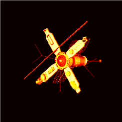
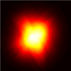
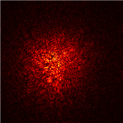
Figure 1: Data produced by the test problem PRblurspeckle, with the true image scene shown on the left, the blurred image scene shown in the middle, and the PSF (which defines the matrix A) shown on the right. The PSF is displayed on a square root scale.

3.2 Inverse Interpolation

Inverse interpolation – also known as gridding – is the problem of computing the values of a function on a regular grid, given function values on arbitrarily located points, in such a way that interpolation of the gridded function values (the unknowns) produces the given values (the data) [21]. This is obviously an inverse problem whose specifics depend on the type of interpolation being used. A different algorithm than ours is implemented in MATLAB’s griddata function.

As a simple example, consider linear interpolation on a 1D grid with grid points $t_{j}^{\mathrm{G}}$, $j=1,2,\ldots$ and data $(t_{i},b_{i})$ on the arbitrary points $t_{1}<t_{2}<t_{3}<\ldots$; then the unknown function values $x_{j}$ at the grid points must satisfy the interpolation relations (for all $i$):

$$b_{i}=x_{j}+\frac{t_{i}-t_{j}^{\mathrm{G}}}{t_{j+1}^{\mathrm{G}}-t_{j}^{\mathrm{G}}}\,(x_{j+1}-x_{j}),\quad\hbox{where}\quad t_{i}\in\left[\,t_{j}^{\mathrm{G}}\,,\,t_{j+1}^{\mathrm{G}}\,\right].$$

This gives a simple linear system of equations $A\,x=b$ with a sparse coefficient matrix $A$ (two nonzeros per row). Note that $A$ is rank deficient if there are consecutive grid intervals with no data points.

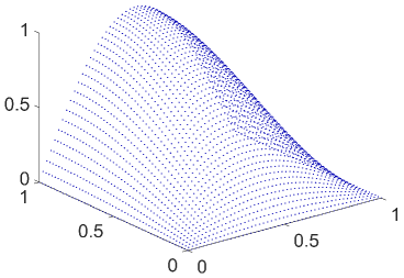
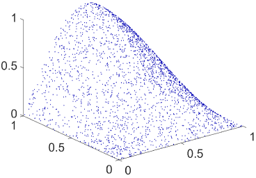
Figure 2: Illustration of the 2D inverse interpolation problem PRinvinterp2 with n = 50. Left: the true solution $x$ defined on a regular grid. Right: the data $b$ defined on randomly scattered points.

Our test problem PRinvinterp2 involves a regular 2D grid with $N=\mathtt{n}^{2}$ grid points $(s_{j}^{\mathrm{G}},t_{j}^{\mathrm{G}})$ generated by meshgrid(linspace(0,1,n)), and there are $M=N$ data points $(s_{i},t_{i})$ randomly distributed in $[0,1]\times[0,1]$. The data values $b_{i}$ at the random points, as well as the true solution $x_{j}$ at the grid points, are samples of the smooth function $\phi(s,t)=\sin(\pi s)\,\sin(\pi/2\,t)$. See Figure 2 for an illustration; the figures are generated with PRshowx and PRshowb after constructing the default test data, that is with the following lines of MATLAB code:

   [A, b, x, ProbInfo] = PRinvinterp2;
   PRshowx(x, ProbInfo)
   PRshowb(b, ProbInfo)

The default value of n is 128, but test data with other values of n can be easily generated by specifying this value directly as an input to the function, e.g.,

   [A, b, x, ProbInfo] = PRinvinterp2(256);

The options structure has only one field, options.InterpMethod, which can be used to choose one of four different types of interpolation: nearest-neighbour, linear (default), cubic, and spline. For example, to use the default value of n $=128$, but the optional cubic interpolation, use the following code:

   options = PRset(’InterpMethod’, ’cubic’);
   [A, b, x, ProbInfo] = PRinvinterp2(options);

The forward computation (corresponding to multiplication with $A$) is always done by means of MATLAB’s interp2 function, and thus A is not constructed explicitly as a matrix, but instead is represented by a function handle. In this test problem we also provide the adjoint operation, so the function handle A can be used to compute matrix-vector multiplications with both $A$ and $A^{T}$. As was mentioned in the previous test problem, all of the iterative methods that we provide in the package do not need any additional information from the user. In case users would like to test their own iterative algorithms, we recall that matrix-vector multiplications with $A$ and $A^{T}$ can be computed using simple function calls. For example, $r=A^{T}(b-Ax)$ can be computed as

   r = A(b - A(x, ’notransp’), ’transp’);

In addition, to get the effective size of A (that is, if it could be constructed explicitly), use the MATLAB statement

   dims = A([], ’size’);

With the default value n = 128, the result is dims = [16384, 16384]. Because the adjoint operation (corresponding to $A^{T}$) is coded by us, it is not necessary to use transpose-free methods with this test problem.

3.3 Inverse Diffusion

Many inverse PDE problems, such as parameter identification in electrical impedance tomography, are nonlinear. For this package we provide a simple linear PDE test problem where the solution is represented on a finite-element mesh and the forward computation involves the solution of a time-dependent PDE. The underlying problem is a 2D diffusion problem in the domain $[0,T]\times[0,1]\times[0,1]$ in which the solution $u$ satisfies

$$\frac{\partial u}{\partial t}=\nabla^{2}u$$ (8)

with homogeneous Neumann boundary conditions and a smooth function $u_{0}$ as initial condition at time $t=0$. The forward problem maps $u_{0}$ to the solution $u_{T}$ at time $t=T$, and the inverse problem is then to reconstruct the initial condition from $u_{T}$, cf. [30].

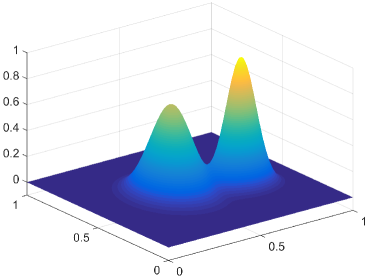
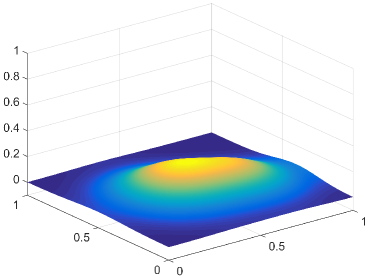
Figure 3: Illustration of the 2D inverse diffusion problem PRdiffusion with n = 64. Left: the true solution $x$ corresponding to the initial function $u_{0}$. Right: the data $b$ corresponding to the function $u_{T}$ at time $T=0.01$.

We discretize the function $u$ on a uniform finite-element mesh with $2(n-1)^{2}$ triangular elements; think of the domain as an $(n-1)\times(n-1)$ pixel grid with two triangular elements in each pixel. Then $u$ is represented by the $N=n^{2}$ values at the corners of the elements. The forward computation – represented by the function handle A – is the numerical solution of the PDE (8), and it is implemented by the Crank-Nicolson-Galerkin finite-element method.

The true solution $x$ and the right-hand side $b$ consist of the $N$ values of $u_{0}$ and $u_{T}$, respectively, at the corners of the elements; see Figure 3 for an example, which was generated using the statement:

   [A, b, x, ProbInfo] = PRdiffusion;

This basic call uses the default input value of n =128, and sets default values for options, which includes

• options.TFinal is the diffusion time (default is 0.01).

• options.Tsteps is the number of time steps (default is 100).

As previously stated, A is returned as a function handle that can be used to perform matrix-vector multiplications. As will be illustrated in Section 4, all of the iterative methods that we provide in the package do not require any additional information from the user. In case users would like to use this test problem in their own iterative algorithms, we recall that matrix-vector multiplications can be computed using a simple function call. For example, to compute $r=b-A\,x$, use the MATLAB statement

   r = b - A(x, ’notransp’);

Note that if A could be constructed explicitly, it would be an $N\times N$ matrix, where $N=n^{2}$. The following MATLAB statement can be used to determine this information:

   dims = A([], ’size’);

thus, with the default value of n = 128, N= 16384.

As with other test problems in this package, an alternate value for n can be directly specified as an input to PRdiffusion. For example, if we want to use n = 256, and default values for options, then we can simply call PRdiffusion as follows:

   [A, b, x, ProbInfo] = PRdiffusion(256);

In addition, the default values for options can easily be changed using PRset. For example, if we want to use n = 256, a diffusion time of 0.3, and 50 time steps, then we type:

   options = PRset(’TFinal’, 0.3, ’Tsteps’, 50);
   [A, b, x, ProbInfo] = PRdiffusion(256, options);

3.4 NMR Relaxometry

Nuclear Magnetic Resonance (NMR) relaxometry consists of reconstructing a distribution of relaxation times associated with the probed material, starting from a signal measured at given times. Two-dimensional (2D) NMR relaxometry can be performed using particular excitation sequences and acquisition strategies, so that the joint distribution of the longitudinal and transverse relaxation times $T^{1}$ and $T^{2}$ can be recovered, providing more chemical information about the probed material than its one-dimensional analogous [31]. 2D NMR relaxometry is mathematically modeled using the following Fredholm integral equation of the first kind

$$\int_{0}^{\widehat{T}^{2}}\int_{0}^{\widehat{T}^{1}}k(\tau^{1},\tau^{2},T^{1},T^{2})\,f(T^{1},T^{2})\,dT^{1}\,dT^{2}=g(\tau^{1},\tau^{2})\,,$$ (9)

where $g(\tau^{1},\tau^{2})$ is the noiseless signal as a function of experiment times $(\tau^{1},\tau^{2})$, and $f(T^{1},T^{2})$ is the density distribution function. The kernel $k(\tau^{1},\tau^{2},T^{1},T^{2})$ in equation (9) is separable and given by

$$k(\tau^{1},\tau^{2},T^{1},T^{2})=\left(1-2\exp(-\tau^{1}/T^{1})\right)\exp(-\tau^{2}/T^{2})\,,$$

and, upon variable transformation, it can be regarded as a Laplace kernel. Perturbations arising in 2D NMR relaxometry measurements are typically modeled as Gaussian white noise. Common techniques to regularize the inversion process include the incorporation of box constraints and smoothness priors on the solution [5].

We discretize the integral in (9) using the the midpoint quadrature rule with logarithmically equispaced nodes

$$T^{1}_{1},T^{1}_{2},\dots,T^{1}_{n_{1}}\quad\mbox{and}\quad T^{2}_{1},T^{2}_{2},\dots,T^{2}_{n_{2}}\,,$$

and considering a corresponding change of variables. We then enforce collocation on the logarithmically equispaced sampled values

$$\tau^{1}_{1},\tau^{1}_{2},\dots,\tau^{1}_{m_{1}}\quad\mbox{and}\quad\tau^{2}_{1},\tau^{2}_{2},\dots,\tau^{2}_{m_{2}}\,,$$

so that equation (9) can be discretized as

$$A^{1}\,X\,(A^{2})^{T}=B\,,$$ (10)

where

$$\begin{array}[]{llll}A^{1}_{\ell_{1},k_{1}}&=&1-2\exp(-\tau^{1}_{\ell_{1}}/T^{1}_{k_{1}})\,,&\quad\ell_{1}=1,\dots,m_{1}\,,\;k_{1}=1,\dots,n_{1}\,,\\ A^{2}_{\ell_{2},k_{2}}&=&\exp(-\tau^{2}_{\ell_{2}}/T^{2}_{k_{2}})\,,&\quad\ell_{2}=1,\dots,m_{2}\,,\;k_{2}=1,\dots,n_{2}\,,\\ B_{\ell_{1},\ell_{2}}&=&g(\tau^{1}_{\ell_{1}},\tau^{2}_{\ell_{2}})\,,&\quad\ell_{1}=1,\dots,m_{1}\,,\;\ell_{2}=1,\dots,m_{2}\,,\\ X_{k_{1},k_{2}}&=&f(T^{1}_{k_{1}},T^{2}_{k_{2}})\,,&\quad k_{1}=1,\dots,n_{1}\,,\;k_{2}=1,\dots,n_{2}\,.\end{array}$$

Equation (10) is a consequence of the fact that the kernel in (9) is separable. Taking $M=m_{1}m_{2}$ and $N=n_{1}n_{2}$, and defining $x\in\mathbb{R}^{N}$ and $b\in\mathbb{R}^{M}$ as the vectors obtained by stacking the columns of $X\in\mathbb{R}^{n_{1}\times n_{2}}$ and $B\in\mathbb{R}^{m_{1}\times m_{2}}$, respectively, we obtain the linear system (1). Due to the separability of the kernel $k$ the matrix $A$ has Kronecker structure, $A=A_{2}\otimes A_{1}$; we do not construct $A$ explicitly, but instead use a function handle that implements matrix-vector multiplications with $A$ and $A^{T}$ through the relation $(A_{2}\otimes A_{1})\,x=\mathrm{vec}\bigl{(}A^{1}\,X\,(A^{2})^{T}\bigr{)}$. The function to construct this example is PRnmr and, like other applications in our package, is called using:

   [A, b, x, ProbInfo] = PRnmr(n, options);

The input parameter n specifies the size of the relaxation time distribution to be recovered, and can either be an integer scalar, in which case it is assumed that n $=n_{1}=n_{2}$, or a vector n $=[n_{1},\;n_{2}]$. The default value is n = 128.

As with the previous example, since A is a function handle, to compute $r=A^{T}(b-A\,x)$ (e.g., for users who want to use this problem to test their own iterative methods) we can use the MATLAB statement

   r = A(b - A(x, ’notransp’), ’transp’);

and the effective size of A can be obtained as

   dims = A([], ’size’);

With the default value of n $=128$, this returns dims = [65536, 16384].

The options structure can be used to change other default parameters, including:

• options.numData is the number of acquired measurements, $m_{1}$ and $m_{2}$. Default is $m_{1}=2n_{1}$ and $m_{2}=2n_{2}$.

• options.material specifies the phantom for the relaxation time distribution, which can be set to be ’carbonate’ (default), ’methane’, ’organic’ or ’hydroxyl’. The chosen phantom is returned as the vector x.

• options.Tloglimits is an array with two values, [Tlogleft, Tlogright], that define the limits for the logarithm of the relaxation times $T$, where

  $T^{1}$ = logspace(Tlogleft, Tlogright, $n_{1}$),

  $T^{2}$ = logspace(Tlogleft, Tlogright, $n_{2}$),

  The default is $[-4,\;1]$.

• options.tauloglimits is an array with two values, [taulogleft, taulogright], that define the limits for the logarithm of the relaxation times $T$, where

  $\tau^{1}$ = logspace(taulogleft, taulogright, $m_{1}$),

  $\tau^{2}$ = logspace(taulogleft, taulogright, $m_{2}$),

  The default is $[-4,\;1]$.

The plots shown in Figure 4 were obtained by using PRshowx and PRshowb to display the data produced from the most basic call to PRnmr with default choices for n and options; that is,

   [A, b, x, ProbInfo] = PRnmr;
   PRshowx(x, ProbInfo)
   PRshowb(b, ProbInfo)

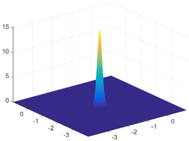
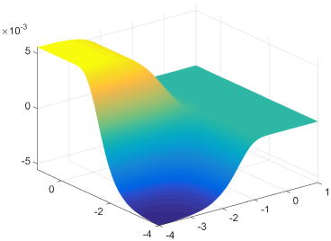
Figure 4: Illustration of the NMR relaxometry problem PRnmr with problem size n = 128. Left: the true solution $x$ as a function of $(\log_{10}(T^{1}),\log_{10}(T^{2}))$. Right: the data $b$ as a function of $(\log_{10}(\tau^{1}),\log_{10}(\tau^{2}))$.

3.5 Tomography

Tomographic reconstruction problems come in many different forms, and we provide three different types of such problems, which can generate data using one of the following three statements:

   [A, b, x, ProbInfo] = PRtomo(n, options);
   [A, b, x, ProbInfo] = PRspherical(n, options);
   [A, b, x, ProbInfo] = PRseismic(n, options);

All three problems are from the AIR Tools II package and we refer to [25] for more details and pictures of the test images. In each case the default value of n determines the size of x (specifically, $x$ represents an $n\times n$ image). The fields that can be specified in options depend on the kind of tomography taken into account.

PRtomo is used to generate test problems that model X-ray attenuation tomography, often referred to as computed tomography (CT). This kind of tomography plays a large role in medical imaging and materials science. The data consists of measurements of the damping of X-rays that penetrate the object and, to a good approximation, can be assumed to travel along straight lines; see [6] for details and mathematical models. The goal is then, from the data, to reconstruct an image of the object’s spatially varying attenuation coefficient.

Since each ray only traverses a small number of the total amount of image pixels, the matrix $A$ will be very sparse (for an $n\times n$ image there are at most $2n$ nonzero elements per row of $A$). We provide two different measurement geometries (there are many more in practice):

• options.CTtype = ’parallel’ (default) gives a parallel-beam tomography where, for each source-detector position angle, there are a number of equidistantly spaced parallel X-rays. This is the typical geometry in synchrotron X-ray measurements, and it corresponds to the well-known Radon transform.

• options.CTtype = ’fancurved’ gives, for each source-detector position angle, a fan of X-rays from a single source to a curved detector, with an identical angular span between all the rays. This is often the case in large medical X-ray scanners.

The data is usually organized as an image called the sinogram, in which each column consists of the data for one source-detector position angle. The user can choose the number of angles, the number of rays per angle, etc.

PRspherical is used to generate test problems that model spherical means tomography. This kind of tomography arises, e.g., in photo-acoustic imaging based on the spherical Radon transform, where the data consists of integrals along circles whose centers are located outside the object. The goal is to reconstruct an image of the initial pressure distribution inside the object (caused by a laser stimulation). Since each circle only intersects a small number of image pixels, the matrix $A$ is sparse. The data is organized in a sinogram-like image whose columns are the data for each circle center. The user can choose the number of circle centers and the number of concentric integration circles per center.

PRseismic is used to generate test problems that model seismic travel-time tomography. This type of tomography uses measurements of the delay of seismic waves to reconstruct an image of the slowness (the reciprocal of the sound speed) in the domain of interest. In our model problem, the sensors are located along two edges of the image (corresponding to the surface and one bore hole) while the wave sources are located along a third edge (corresponding to another bore hole). We provide two different models of the seismic wave:

• options.wavemodel = ’ray’ (default) corresponds to an assumption that the wave frequency is infinite, such that the waves can be well represented by straight lines (similarly to X-ray tomography).

• options.wavemodel = ’fresnel’ corresponds to a model with a finite wave frequency, where it is assumed that the wave is confined to its first Fresnel zone – a cigar-shaped domain with its endpoints at the source and the detector.

Similarly to X-ray tomography, in both cases we obtain a sparse matrix, which is more sparse for the line model. We organize the data in an image where each column contains all the measurements from one source. Since A is a sparse matrix for all the tomography test problems, standard MATLAB operators for multiplication, transpose, etc., can be used.

3.6 The Severity of the Test Problems

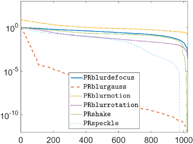
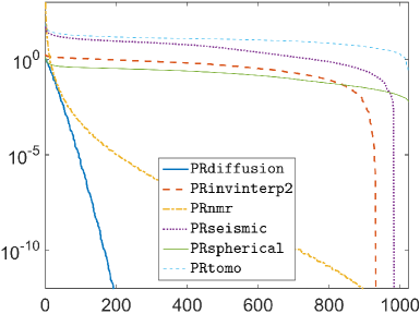
Figure 5: The singular values of the matrix $A$ for all 12 test problems in this package, for $n=32$ and using default options. PRblurgauss, PRdiffusion and PRnmr are severely ill posed, the remaining problems are mildly ill posed.

It is convenient to have a measure of the severity of the test problems included in this package. In linear algebra this is often measured by the condition number of the matrix $A$, but the decay of the singular values of $A$ is a much better measure of the severity of the underlying problem: the faster the decay the severer the problem (and hence the larger the condition number); see, e.g., [22].

Figure 5 shows the singular values of $A$ for all 12 test problems, for the particular choice $n=32$ and using default options. Note that the fast decay of the singular values towards $N=n^{2}=1024$, observed for most problems, is a discretization artifact. The severely ill-posed problems are image deblurring with a Gaussian PSF, the inverse diffusion problem, and the NMR relaxometry problem; the remaining problems are mildly ill posed. The help lines in the PR___ functions describe which problem parameters affect the problem’s severity.

3.7 Adding Noise to the Data

We also provide a function in order to make it easy to add noise to the data $b$:

   [bn, NoiseInfo] = PRnoise(b, NoiseLevel, kind);

where the output bn = b + noise is the noisy data; noise is the vector of perturbations, and it is available within the output structure NoiseInfo. As is the case with other PR___ functions, PRnoise can be called without specifying any input, in which case default values are used. The noise is scaled such that

$$\|\mathtt{noise}\|_{2}/\|\mathtt{b}\|_{2}=\mathtt{NoiseLevel}$$ (11)

with the default NoiseLevel = 0.01. We provide three different kinds of noise that can be easily obtained by setting the following options:

• kind = ’gauss’ (default) gives Gaussian white noise, $\mathtt{noise(i)}\sim\mathcal{N}(0,\sigma^{2})$, with zero mean and with the standard deviation $\sigma$ chosen to satisfy (11): This noise is easily generated by means of:

     [bn, NoiseInfo] = PRnoise(b, NoiseLevel, ’gauss’);
  

• kind = ’laplace’ gives Laplacian noise, $\mathtt{noise(i)}\sim\mathcal{L}(0,\beta)$, with zero mean, and the scale parameter $\beta$ is chosen to satisfy (11). This noise is easily generated by means of:

     [bn, NoiseInfo] = PRnoise(b, NoiseLevel, ’laplace’);
  

• kind = ’multiplicative’ gives a specific type of multiplicative noise (often encountered in radar and ultrasound imaging [14]) where each element bn(i) equals b(i) times a random variable following a Gamma distribution $\mathrm{\Gamma}(\kappa,\theta)$ with mean $\kappa\,\theta=1$ and the parameter $\kappa$ chosen such that (11) is approximately satisfied:

     [bn, NoiseInfo] = PRnoise(b, NoiseLevel, ’multiplicative’);
  

Information about the kind of generated noise and its level are available within the output structure NoiseInfo. Note that PRnoise makes use of MATLAB’s random number generator functions, and thus to construct repeatable experiments (i.e., to generate the same bn for multiple experiments), users should use MATLAB’s rng function to control the seed of the random number generator before calling PRnoise.

Other types of noise can be added by means of the function imnoise from MATLAB’s Image Processing Toolbox.

While Poisson noise is also a common type of noise in imaging, it is not included in this package because it does not conform to the use of PRnoise. Specifically, in the presence of Poisson noise each noisy data element bn(i) is an integer random variable following the Poisson distribution $\mathcal{P}(\mathtt{b(i)})$, i.e., the noise-free data element b(i) is both the mean and the variance of bn(i). Hence, if we want to scale the “noise” vector $\mathtt{noise}=\mathtt{bn}-\mathtt{b}$ then we can only do this by scaling the noise-free data vector $\mathtt{b}$ and the solution vector x accordingly (the scaling factor can be found, e.g., by a simple fixed-point scheme. Poisson noise can also be incorporated by means of poissrnd from the Statistics Toolbox.

Another important type of noise, which arises in X-ray computed tomography, can be referred to as “log-Poisson” (not a standard name). Here the noisy elements of the right-hand side in the linear model (1) are given by $b_{i}=\log(\tilde{d}_{i})$ with $\tilde{d}_{i}\sim\mathcal{P}(d_{i})$, where $d_{i}$ is the expected photon count for the $i$th measurement. It can be shown that $\log(\tilde{d}_{i})$ approximately follows the normal distribution $\mathcal{N}(\log(d_{i}),d_{i}^{-1})$ (corresponding to a quadratic approximation of the associated likelihood function, cf. [37]). This provides a simple way to generate reasonably realistic noise for X-ray tomography problems of the form (1) with the code:

   noise = randn(size(b))./sqrt(b);
   bn    = b + noise;

Again, note that one must scale the noise-free $\mathtt{b}$ in order to scale the relative noise level.

4 Examples and Demonstrations

In this section we demonstrate the use of the iterative reconstruction methods and the test problems by means of some numerical examples. Scripts to run these examples are available in IR Tools with the naming convention EX___.

4.1 Solving 2D Image Deblurring Problems with CGLS and Hybrid Methods

Here we illustrate the use of IRcgls and IRhybrid_lsqr using the speckle image deblurring example PRblurspeckle described in Section 3.1. We use the default image size of n = 256 (i.e., the true and blurred images have $256\times 256$ pixels), the default true image (Hubble Space Telescope), the default level of blurring (moderate), and we add 1% Gaussian noise; specifically, we generate the data using the following lines of MATLAB code:

   NoiseLevel = 0.01;
   [A, b, x, ProbInfo] = PRblurspeckle;
   [bn, NoiseInfo] = PRnoise(b, ’gauss’, NoiseLevel);

Figure 6 shows the resulting true image x (Fig. 6a) and the blurred and noisy image bn (Fig. 6b).

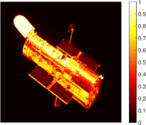
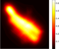
(a)	(b)

Figure 6: Image blurring test data for the example in Section 4.1: (a) true image, (b) blurred and noisy image.

We begin by running IRcgls for 100 iterations, saving only the iteration satisfying the stopping criterion; we use the input options to provide the true solution to IRcgls, so that we can investigate how the relative errors behave at each iteration. Specifically:

   options = IRset(’x_true’, x);
   [X, IterInfo_cgls] = IRcgls(A, bn, options);

Note that in this example we do not specify a maximum number of iterations, so the method uses the default value 100. The output X contains the solution at the final iteration; in this example, convergence criteria are not satisfied, so the method runs the full 100 iterations, and thus X is the solution at iteration 100. Also note that because we specified the true solution x in options, the relative errors $\|x^{(k)}-\mathtt{x}\|_{2}/\|\mathtt{x}\|_{2}$ at each iteration are saved in the output structure, IterInfo_cgls.Enrm. A plot of the relative errors can then be easily displayed as

   plot(IterInfo_cgls.Enrm)

From this plot, which is shown by the blue solid curve in Figure 7, we observe the well-known semi-convergence behavior of CGLS, and we can also observe that the smallest relative error occurs at iteration 39 (denoted by the red circle in the plot). We refer to the solution where the relative error is minimized as the “best regularized solution.” One feature of our iterative methods is that if the true solution is provided through the options structure, then in addition to computing error norms, this best regularized solution is also saved in IterInfo_cgls.BestReg.X, and the iteration where the error is smallest can be found in IterInfo_cgls.BestReg.It. Thus, if we want to display this solution where the error is minimized, we can use PRshowx as follows:

   PRshowx(IterInfo_cgls.BestReg.X, ProbInfo)

This solution is shown in Figure 8a.

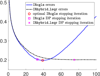
Figure 7: Relative error plot for the image deblurring test problem from the example in Section 4.1. The blue solid curve displays the iteration history (relative errors) of IRcgls, the red circle marks iteration 39 where the IRcgls relative error is at its minimum value, and the magenta square marks iteration 33 which is the IRcgls stopping iteration chosen by the discrepancy principle. The black dashed curve is the iteration history (relative errors) of IRhybrid_lsqr, and the magenta $\times$ marks iteration 75 which is the IRhybrid_lsqr stopping iteration chose by when using the weighted GCV ’wgcv’ parameter-choice method for the projeted problem.

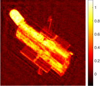
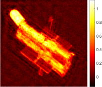
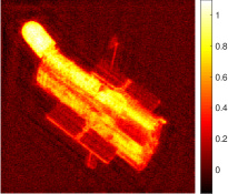
(a)	(b)	(c)

Figure 8: Restored images from the example in Section 4.1: (a) restored image using 39 iterations of IRcgls, (b) restored image after 33 iterations of IRcgls, (c) restored image after 75 iterations of IRybrid_lsqr.

Using the true solution to determine a stopping iteration is cheating, but our implementations can use other schemes that do not require knowing the true image. For example, if we know the noise level in the data, then that information can be used along with the discrepancy principle to determine a stopping iteration. To do this, we simply need to change the options, and run IRcgls; specifically,

   options = IRset(options, ’NoiseLevel’, NoiseLevel);
   [X, IterInfo_cgls_dp] = IRcgls(A, bn, options);

We emphasize that the previously set options remain unchanged – only the one that is specified (in this example ’NoiseLevel’) is changed. Now the discrepancy principle terminates IRcgls at iteration 33. The relative error at this iteration is shown by the magenta square in Figure 7. It is well-known that the discrepancy principle tends to compute overly smooth solutions, but this is not the case here where we know the exact error norm, and we are able to compute the good restoration shown in Figure 8b.

We conclude this subsection by illustrating the use of one of the hybrid methods, namely IRhybrid_lsqr. This scheme enforces regularization at each iteration, and thus avoids the semi-convergence behavior seen in IRcgls. In order to illustrate an approach that does not require an estimate of the error norm, we use the weighted GCV ’wgcv’ parameter-choice method (which is default) for the projected problem. Specifically, if we use IRhybrid_lsqr and if we properly modify the information about the regularization parameter choice in the previously defined options,

    options = IRset(options, ’RegParam’, ’wgcv’);
    [X, IterInfo_hybrid] = IRhybrid_lsqr(A, bn, options);

the method terminates at iteration 75 (which can be found from the output structure IterInfo_hybrid.its).

If we want to show that IRhybrid_lsqr avoids the semi-convergence behavior, we need to force the method to run more iterations, past the recommended stopping iteration. We can do this by using an additional NoStop specification in the options. That is,

   options = IRset(options, ’NoStop’, ’on’);
   [X_hybrid, IterInfo_hybrid] = IRhybrid_lsqr(A, bn, options);

With the NoStop option turned ’on’, the iterations continue to the default maximum of 100. In this case, the vector X_hybrid is the solution at iteration 100, but we also save the solution at the recommended stopping iteration in the output structure, IterInfo_hybrid.StopReg.X, and the iteration where the stopping criterion is satisfied is saved in IterInfo_hybrid.StopReg.It. Note that the field StopReg is different than the field BestReg: the former stores information about the solution that satisfies the stopping criterion; the latter stores information about the best computed solution (and requires x_true to be specified among the input options). The relative errors for 100 iterations of IRhybrid_lsqr are shown in the black dashed curve of Figure 7, with the recommended stopping iteration denoted by the magenta $\times$. The solution at this recommended stopping iteration is shown in Figure 8c.

The code used to generate the test problem and results described in this example is provided in our package in the script EXblur_cgls_hybrid.m.

4.2 Solving the 2D Inverse Interpolation Problem with Priorconditioned CGLS

Here we use the 2D inverse interpolation test problem PRinvinterp2 to illustrate how to use prior-conditioning in IRcgls. We begin by generating the test problem using n $=32$, and add 5% Gaussian noise:

   n = 32;
   [A, b, x, ProbInfo] = PRinvinterp2(n);
   bn = PRnoise(b, 0.05);

The true solution x and data b were already shown in Section 3.2, Figure 2; the data bn looks very similar to b. We attempt to solve this problem with three different versions of CGLS:

• Standard CGLS, using the statement:

     K = 1:200;
     [X1, IterInfo1] = IRcgls(A, bn, K);
  

  Unfortunately, without providing additional information, CGLS cannot recognize an appropriate stopping iteration, and the final computed solution is a poor approximation; see Figure 9a.

• Priorconditioned CGLS with options.RegMatrix = ’Laplacian2D’ which enforces zero boundary conditions everywhere. This can be computed using

     options.RegMatrix = ’Laplacian2D’;
     [X2, IterInfo2] = IRcgls(A, bn, K, options);
  

  In this case, CGLS finds a smoother solution that somewhat resembles the exact solution in half of the domain. But in the other half, the solution (while still smooth) is incorrect due to the zero boundary condition at that edge where the exact solution is nonzero. This is clearly seen in Figure 9b.

• We can also create our own prior-conditioning matrix $L$. Specifically we construct a matrix $L$ that is similar to the 2D Laplacian, except we enforce a zero derivative on one of the boundaries;

     L1 = spdiags([ones(n,1),-2*ones(n,1),ones(n,1)],[-1,0,1],n,n);
     L1(1,1:2) = [1,0]; L1(n,n-1:n) = [0,1];
     L2 = L1; L2(n,n-1:n) = [-1,1];
     L = [ kron(speye(n),L2) ; kron(L1,speye(n)) ];
     L = qr(L,0);
     options.RegMatrix = L;
     [X3, IterInfo3] = IRcgls(A, bn, K, options);
  

  In this case, the iteration terminates after $k=10$ iterations, and because the prior-conditioner enforces correct boundary conditions, we obtain a very good computed approximation; see Figure 9c.

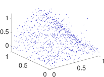
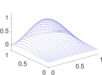
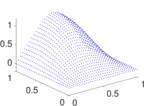
(a)	(b)	(c)

Figure 9: Illustration of the solution of the 2D inverse interpolation problem PRinvinterp2 with n = 32 by means of IRcgls and with three different regularization matrices: (a) the identity gives a very noisy solution, (b) the 2D Laplacian with zero boundary conditions everywhere gives a smooth but incorrect solution, (c) enforcing instead a zero derivative on the boundary where the solution is nonzero gives a good approximate solution.

In this example, we rely on the default normal equations residual for the stopping rule, $\|A^{T}(b-A\ x^{(k)})\|_{2}/{\|A^{T}b\|_{2}}\leq\mathtt{options.NE\_Rtol}=10^{-12}$, where $x^{(k)}$ is the computed approximate solution at iteration $k$. We also remark that in each of the calls to IRcgls, the third input argument K = 1:200 is used to request that the methods return all solution iterates in X1, X2 and X3. For example, since the first call to IRcgls runs all 200 iterations, X1 is an array of size ${1024}\times 200$, but since the other two calls only needed 5 iterations, X2 and X3 are arrays of size ${1024}\times 5$. This can be very useful if one wants to view solutions at earlier iterations. For example, it would be very easy to see how the solution at iteration 5 of the first call to IRcgls compares with second two calls, e.g.,

   PRshowx(X1(:,5), ProbInfo)

However, requesting all the solution iterates can lead to a large amount of storage, especially when solving very large problems, so we caution users to use this capability wisely. For example, K can be any set of integers, such as K = [1, 10:10:200], which would return solutions at iterations $1,\,10,\,20,\,\ldots,\,{200}$.

The code used to generate the test problem and results described in this example is provided in our package in the script EXinvinterp2_cgls.m.

4.3 Solving the 2D Inverse Diffusion Problem with RRGMRES

This example illustrates the use of IRrrgmes which does not require operations with the adjoint operator (the matrix transpose). We consider the 2D inverse diffusion problem from §3.3 in PRdiffusion. As with previous examples in this section, we begin by setting up the test problem:

   n = 64;
   NoiseLevel = 0.005;
   [A, b, x, ProbInfo] = PRdiffusion(n);
   [bn, NoiseInfo] = PRnoise(b, NoiseLevel);

The true solution x and data bn are shown in Figure 10a and Figure 10d, respectively. We now use RRGMRES to solve the problem, but first we set a few options by modifying the appropriate fields in the option structure:

• First, we set options.x_true to the true solution x which allows the method to compute relative error norms.

• Next, we want to use the discrepancy principle as stopping rule, so we need to set options.NoiseLevel. We also change the default safety parameter eta to be 1.01.

• Finally, we turn on the option NoStop so that the iteration will proceed to the maximum number of iterations, even if a stopping criterion is satisfied.

As mentioned earlier, all these parameters can be set in a single call to IRset,

   options = IRset(’x_true’, x, ’NoiseLevel’, NoiseLevel, ...
         ’eta’, 1.01,’NoStop’, ’on’);

We can then use RRGMRES as follows:

   [X, IterInfo] = IRrrgmres(A, bn, K, options);

Once the iterations are completed, we can access several pieces of information from the structure IterInfo. Specifically,

• IterInfo.Enrm contains the relative error norms, which are displayed in Figure 10b.

• The “best regularized solution” is saved in IterInfo.BestReg.X, and the iteration where the error is smallest can be found in IterInfo.BestReg.It. This solution is shown in Figure 10e.

• IterInfo.Rnrm contains the relative residual norms at each iteration,$\|b-A\,x^{(k)}\|_{2}{/\|b\|_{2}}$, which are displayed in Figure 10c, along with a line marking the stopping point defined by the discrepancy principle. That is, once the residual norm reaches the red dashed line, the convergence criterion defined by the discrepancy principle is considered satisfied.

• The precise iteration satisfying the stopping criterion, along with its corresponding solution, can be obtained from IterInfo.StopReg.It andIterInfo.StopReg.X, respectively. This solution is shown in Figure 10f.

We again emphasize that all the iterative methods implemented in our package have a similar input and output structure.

The code used to generate the test problem and results described in this example is provided in our package in the script EXdiffusion_rrgmres.m.

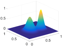
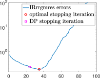
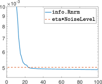
(a)	(b)	(c)
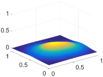
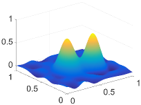
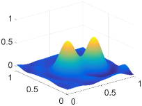
(d)	(e)	(f)

Figure 10: Illustration of the solution of the 2D inverse diffusion problem PRdiffusion with n = 64 by means of IRrrgmres. We set options.NoStop = ’on’ to force the iterations to continue beyond the number of iterations selected by the discrepancy principle stopping rule. (a) true solution x, (b) relative error history, (c) relative residual norm history, (d) noisy data bn, (e) best reconstruction ($k=35$), (f) reconstruction obtained when the discrepancy principle is satisfied ($k=24$).

4.4 Solving the 2D NMR Relaxometry Problem with MRNSD

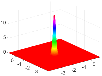
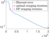
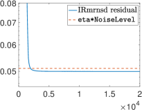
(a)	(b)	(c)
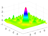
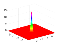
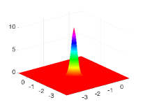
(d)	(e)	(f)

Figure 11: Illustration of the solution of the 2D NMR relaxometry problem PRrmn with n = 64 by means of IRmrnsd. We use a color map that emphasizes the behavior of the large flat region. We set options.NoStop = ’on’ to force the iterations to continue beyond the number of iterations selected by the discrepancy principle stopping rule. (a) true solution x, (b) relative error history, (c) relative residual norm history, (d) best reconstruction by CGLS ($k=94$), (e) best reconstruction by MRNSD ($k=19999$), (f) reconstruction obtained by MRNSD when the discrepancy principle is satisfied ($k=1950$).

To demonstrate the advantage of imposing nonnegativity constraints we consider the 2D NRM relaxometry problem from §3.4 implemented in PRnmr, with n = 64. As done for the other test problems, we begin by setting

   n = 64;
   NoiseLevel = 0.05;
   [A, b, x, ProbInfo] = PRnmr(n);
   bn = PRnoise(b, NoiseLevel);

The true solution x is shown in Figure 11a. This test problem is extremely hard to solve, and every iterative method available in our package requires a large amount of iterations to compute a meaningful approximation of x. We allow 20000 iterations at most, and we can store one approximate solution every 1000 iterations by setting K = [1, 1000:1000:20000]. We assign the following options by calling the IRset function:

   options = IRset(’x_true’, x, ’NoiseLevel’, NoiseLevel, ...
         ’eta’, 1.01, ’NoStop’, ’on’);

We now use CGLS as follows:

   [X_cgls, IterInfo_cgls] = IRcgls(A, bn, K, options);

The solution computed by means of IRcgls is shown in Figure 11d; this solution hardly resembles the exact one reported in Figure 11a and, more specifically, it has large oscillations and negative values in the part that ideally should be zero.

To run IRmrnsd with the same test data and input options as the ones used for IRcgls we simply type

   [X_mrnsd, IterInfo_mrnsd] = IRmrnsd(A, bn, K, options);

We recall that nonnegativity constraints are automatically imposed within the IRmrnsd iterations. IterInfo_mrnsd stores various pieces of information about the behavior of this solver applied to this test problem. In particular, we can access the relative error at each iteration in IterInfo.Enrm, which is displayed in Figure 11b. The relative residual at each iteration is stored in IterInfo.Rnrm; this is displayed in Figure 11c, together with a horizontal line marking the relative noise level (useful to visually inspect when the discrepancy principle is satisfied). The “best regularized solution” is saved in IterInfo_mrnsd.BestReg.X, and the iteration where the error is smallest can be found in IterInfo_mrnsd.BestReg.It. This solution is shown in Figure 11e. The precise iteration satisfying the discrepancy principle, along with its corresponding solution, can be obtained from IterInfo_mrnsd.StopReg.It and IterInfo_mrnsd.StopReg.X, respectively. This solution is shown in Figure 11f.

The code used to generate the test problem and results described in this example is provided in our package in the script EXnmr_cgls_mrnsd.m.

4.5 Computing Sparse Reconstructions

This example illustrates how to use IRirn and IRell1 to compute approximately sparse reconstructions – in the sense that the solution has many small values (that may consecutively be truncated to zero).

The test problem is Gaussian image deblurring, and we choose one of our synthetically generated images that is made up of randomly placed small “dots”, with random intensities. This test mage may be used, for example, to simulate stars being imaged from ground based telescopes. To generate the test problem, we use the options structure to specify the ’dotk’ synthetic image,

   PRoptions.trueImage = ’dotk’;
   [A, b, x, ProbInfo] = PRblurgauss(PRoptions);

and add $10\%$ white noise,

   NoiseLevel = 0.1;
   bn = PRnoise(b, NoiseLevel);

We then compute the best solutions by means of IRcgls, which cannot impose sparsity, as well as IRell1 and IRirn, which are simplified drivers for IRhybrid_fgmres and IRrestart, respectively. Both IRell1 and IRirn are designed to make it easy to approximately enforce a 1-norm penalization on the solution, leading to a reconstruction with many small elements.

To illustrate the effect of the parameter-choice rule for the projected problem in the hybrid method IRhybrid_fgmres, we use both GCV (which is the default) and the discrepancy principle. If GCV is used, then the iterations stop when the minimum of the iteration-dependent GCV function stabilizes or starts increasing within a given window. If the discrepancy principle is used, the iterations are stopped according to the strategy proposed in [17], and previously addressed in Section 2.5. The regularization parameters for the inner iterations of IRirn are chosen by the discrepancy principle that also acts as a stopping rule for the inner iterations; the default stopping criterion for the outer iterations is the stabilization of the norm of the solution at each restart. However, for all the solvers, we are interested in computing the best solutions, which may be found after the stopping rules are satisfied. For this reason we use the “no stop” feature in IRcgls and IRell1, and the “no stop out” feature in IRirn, so to ensure that the iterations are continued after the stopping criterion (for IRcgls and IRell1) and the outer stopping criterion (for IRirn) are satisfied.

Specifically, first run IRcgls for 80 iterations, using the true solution to compute error norms, and turn NoStop on:

   options = IRset(’MaxIter’, 80, ’x_true’, x, ’NoStop’, ’on’);
   [Xcgls, info_cgls] = IRcgls(A, bn, options);

Now compute a sparse solution using the default GCV rule for choosing the regularization parameter of the projected problem,

   options.NoStop = ’on’;
   [Xell1_GCV, info_ell1_GCV] = IRell1(A, bn, options);

To change the default regularization parameter-choice rule to the discrepancy principle, using the true NoiseLevel with a safety value for eta, we use IRset as follows:

   options = IRset(options, ’RegParam’, ’discrep’, ...
                            ’NoiseLevel’, NoiseLevel, ’eta’, 1.1);
   [Xell1_DP, info_ell1_DP] = IRell1(A, bn, options);

Finally, consider IRirn with the discrepancy principle used for the inner iterations, with NoStopOut turned on, and with 80 total iterations. This can be simply achieved as follows:

   options.NoStopOut = ’on’;
   K = 80;
   [Xirn_DP,info_irn_DP] = IRirn(A, bn, K, options);

Because of the interplay between the inner iterations (whose number depends on the discrepancy principle) and outer iterations, we need to explicitly specify K to ensure that the maximum number of total iterations is 80.

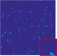
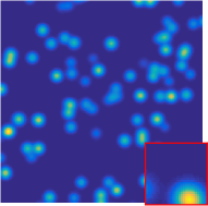
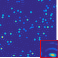
(a)	(b)	(c)
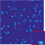
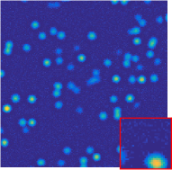
(d)	(e)	(f)

Figure 12: Illustration of sparse solutions to an image deblurring problem generated with PRblur and n $=256$, and with a sparse test image with synthetic stars. (a) true solution x, (b) noisy blurred image bn, (c) best CGLS reconstruction ($k=53$), (d) best IRell1 solution with the default GCV parameter-choice rule for the projected problem ($k=5$), (e) best IRell1 solution with the discrepancy principle parameter-choice rule for the projected problem ($k=51$), (f) best IRirn solution with the discrepancy principle parameter-choice and stopping rule for the inner iterations ($k=4$). All negative pixels are truncated to 0 and the inset figures zoom in on the bottom right $30\times 30$ corner of the image.

Figures 12a and 12b show the true image and the noisy blurred image, respectively. The CGLS reconstruction shown in 12c is clearly contaminated by oscillations (“ringing effects”) around the reconstructed stars, and we also see other artifacts that appear as “freckles” as discussed in [24]. For the reconstructions computed by IRell1 shown in 12d-e, we see that the parameter-choice rule for the projected problem indeed has an effect on the iterations – in this example we obtain the best reconstruction with the discrepancy principle. Also the reconstruction computed by IRirn shown in 12f is successful in computing a sparse solution though, for this test problem, IRell1 exhibits a better performance. This example demonstrates that the heuristic approach to computing a sparse reconstruction in IRell1 works well – as long as one can accept small elements rather than exact zeros in the reconstruction.

The code used to generate the test problem and results described in this example is provided in our package in the script EXsparsity.m.

5 Conclusion

We gave an overview of a MATLAB software package IR Tools that provides large-scale iterative regularization methods and new large-scale test problems. Our package allows the user to easily experiment with a variety of well-documented iterative regularization methods in a flexible and uniform framework, and at the same time our software can be used efficiently for real-data problems. We also provide a set of realistic large-scale 2D test problems that replace the outdated ones from Regularization Tools and that are valid alternatives to the ones available within other popular MATLAB toolboxes and packages.

6 Acknowledgements

The authors are grateful to Julianne Chung for providing an implementation of HyBR, which forms the basis of our IRhybrid_lsqr function. For further details, see [11, 13] and http://www.math.vt.edu/people/jmchung/hybr.html. We also thank Germana Landi for providing insight about the NMR relaxometry problem.

The satellite image in our package, shown in Fig. 1, is a test problem that originated from the US Air Force Phillips Laboratory, Lasers and Imaging Directorate, Kirtland Air Force Base, New Mexico. The image is from a computer simulation of a field experiment showing a satellite as taken from a ground based telescope. This data has been used widely in the literature for testing algorithms for ill-posed image restoration problems; see, for example [35].

Our package also includes a picture of NASA’s Hubble Space Telescope as shown in Fig, 6. The picture is in the public domain and can be obtained from https://www.nasa.gov/mission_pages/hubble/story/index.html.

References

- [1] Andersen, M. S. and Hansen, P. C.: Generalized row-action methods for tomographic imaging. Numer. Algo., 67, 121–144 (2014). doi: 10.1007/s11075-013-9778-8.
- [2] Andrews, H., and Hunt, B.: Digital Image Restoration. Prentice-Hall, Englewood Cliffs, NJ, 1977.
- [3] Beck, A. and Teboulle, M.: A fast iterative shrinkage-thresholding algorithm for linear inverse problems. SIAM J. Imaging Sci., 2, 183–202 (2009).
- [4] Bertero, M., and Boccacci, P.: Introduction to Inverse Problems in Imaging. IOP Publishing Ltd., London, 1998.
- [5] Bortolotti, V., Brown, R. J. S., Fantazzini, P., Landi, G., and Zama, F.: Uniform Penalty inversion of two-dimensional NMR relaxation data. Inverse Problems, 33, 015003 (2016).
- [6] Buzug, T. M.: Computed Tomography. Springer, Berlin, 2008.
- [7] Calvetti, D., Landi, G., Reichel, L., and Sgallari, F.: Non-negativity and iterative methods for ill-posed problems. Inverse Problems, 20, 1747–1758 (2004).
- [8] Calvetti, D., Lewis, B., and Reichel, L.: GMRES-type methods for inconsistent systems. Linear Algebra Appl., 316, 157-–169 (2000).
- [9] Calvetti, D., Morigi, S., Reichel, L., and Sgallari, F.: Tikhonov regularization and the L-curve for large discrete ill-posed problems. J. Comput. Appl. Math., 123, 423–446 (2000).
- [10] Calvetti, D., Reichel, L., and Shuibi, A.: Enriched Krylov subspace methods for ill-posed problems. Lin. Alg. Appl., 362, 257–273 (2003).
- [11] Chung, J.: Numerical Approaches for Large-Scale Ill-Posed Inverse Problems. PhD Thesis, Emory University, Atlanta, GA, May 2009.
- [12] Chung, J., Knepper, S., and Nagy, J. G.: Large-scale inverse problems in imaging. In Scherzer, O. (Ed.): Handbook of Mathematical Methods in Imaging. Springer, Heidelberg, 2011.
- [13] Chung, J., Nagy, J. G., and O’Leary, D. P.: A weighted-GCV method for Lanczos-hybrid regularization. Electronic Transactions on Numerical Analysis, 28, 149–167 (2008).
- [14] Dong, Y., and Zeng, T.: A convex variational model for restoring blurred images with multiplicative noise. SIAM J. Imaging Sciences, 6, 1598–1625 (2013).
- [15] Elfving, T., Hansen, P. C., and Nikazad, T.: Semi-convergence properties of Kaczmarz’s method. Inverse Problems, 30, 055007 (2014). doi: 10.1088/0266-5611/30/5/055007.
- [16] Gazzola, S. and Nagy, J. G.: Generalized Arnoldi-Tikhonov method for sparse reconstruction. SIAM J. Sci. Comput., 36, B225–B247 (2014).
- [17] Gazzola, S. and Novati, P.: Automatic parameter setting for Arnoldi-Tikhonov methods. J. Comput. Appl. Math., 256, 180–195 (2014).
- [18] Gazzola, S., Novati, P., and Russo, M. R.: On Krylov projection methods and Tikhonov regularization. Electron. Trans. Numer. Anal., 44, 83–123 (2015).
- [19] Gazzola, S. and Wiaux, Y.: Fast nonnegative least squares through flexible Krylov subspaces. SIAM J. Sci. Comput., 39, A655–A679 (2017).
- [20] Golub, G. H., Heath, M. T., and Wahba, G.: Generalized cross-validation as a method for choosing a good ridge parameter. Technometrics, 21, 215–223 (1979).
- [21] Guo, L., Meng, X., and Shi, L.: Gridding aeromagnetic data using inverse interpolation. Geophys. J. Internat., 189, 1353-1360 (2012).
- [22] Hansen, P. C.: Discrete Inverse Problems: Insight and Algorithms. SIAM, Philadelphia, 2010.
- [23] Hansen, P. C.: Regularization Tools version 4.0 for Matlab 7.3. Numer. Algo., 46, 189–194 (2007).
- [24] Hansen, P. C. and Jensen, T. K.: Noise propagation in regularizing iterations for image deblurring, Electronic Transactions on Numerical Analysis, 31, 204–220 (2008).
- [25] Hansen, P. C. and Jørgensen, J. S.: AIR Tools II: Algebraic iterative reconstruction methods, improved implementation. Numer. Algor., X, X–X (20XX). doi: 10.1007/s11075-017-0430-x.
- [26] Hansen, P. C., Nagy, J. G., and Tigkos, K.: Rotational image deblurring with sparse matrices. BIT Numerical Mathematics, 54, 649–671 (2014).
- [27] Hansen, P. C., Nagy, J. G., and O’Leary, D. P.: Deblurring Images: Matrices, Spectra and Filtering. SIAM, Philadelphia, PA, 2006.
- [28] Kilmer, M. E., Hansen, P. C., and Español, M. I.: A projection-based approach to general-form Tikhonov regularization. SIAM J. Sci. Comput., 29, 315–330 (2007).
- [29] Lagendijk, R. L., and Biemond, J.: Iterative Identification and Restoration of Images. Kluwer Academic Publishers, Boston/Dordrecht/London, 1991.
- [30] Min, T., Geng, B., and Ren, J.: Inverse estimation of the initial condition for the heat equation. Intl. J. Pure Appl. Math., 82, 581–593 (2013).
- [31] Mitchell, J., Chandrasekera, T. C., and Gladden, L.F.: Numerical estimation of relaxation and diffusion distributions in two dimensions. Prog. Nucl. Magn. Reson. Spectrosc., 62, 34–50 (2012).
- [32] Nagy, J. G., Palmer, K., and Perrone, L.: Iterative methods for image deblurring: A Matlab object oriented approach. Numer. Algor., 36, 73–93 (2004).
- [33] Nagy, J. G. and Strakoš, Z.: Enforcing nonnegativity in image reconstruction algorithms. In Wilson, D. C. (Ed.): Mathematical Modeling, Estimation, and Imaging. Proceedings of SPIE 4121, 182–-190 (2000). doi: 10.1117/12.402439
- [34] Novati, P. and Russo, M. R.: A GCV-based Arnoldi-Tikhonov regularization methods. BIT Numerical Mathematis, 54, 501–521 (2014).
- [35] M. C. Roggemann and B. Welsh: Imaging Through Turbulence. CRC Press, Boca Raton, Florida, 1996.
- [36] Rodríguez, P. and Wohlberg, B.: An efficient algorithm for sparse representations with data fidelity term. Proc. 4th IEEE Andean Technical Conference (ANDESCON), 2008.
- [37] Sauer, K. and Bouman, C.: A local update strategy for iterative reconstruction from projections. IEEE Trans. Signal Proc., 41, 534–548 (1993).
- [38] Vogel, C. R.: Computational Methods for Inverse Problems. SIAM, Philadelphia, 2002.
- [39] Zhdanov, M.: Geophysical Inverse Theory and Regularization Problems. Elsevier, Amsterdam, 2002.