Asymptotics of the contour of the stationary phase and efficient evaluation of the Mellin–Barnes integral for the $\displaystyle F_{3}$ structure function

Abstract

A new approximation is proposed for the contour of the stationary phase of the Mellin–Barnes integrals in the case of its finite asymptotic behavior as $\displaystyle{\rm Re}z\to-\infty$. The efficiency of application of the proposed contour and the quadratic approximation to the contour of the stationary phase is compared by the example of the inverse Mellin transform for the structure function $\displaystyle F_{3}$. It is shown that, although for a small number of terms $\displaystyle N$ in quadrature formulas used to calculate integrals along these contours, the quadratic contour is more efficient, but for $\displaystyle N>20$ the asymptotic stationary phase integration contour gives better accuracy. The case of the $\displaystyle Q^{2}$-dependence of the $\displaystyle F_{3}$ structure function is also considered.

I Introduction

The Mellin–Barnes (MB) integrals Bateman are widely used at high-energy physics. Recently, significant progress has been made in the numerical computation of these integrals. The review of digital packages is presented in the introduction to the paper Gluza:2016fwh . The list of physical tasks solved using the MB integrals (two-loop massive Bhabha scattering in QED, in three-loop massless form factors and static potentials, in massive two-loop QCD form factors, in B-physics studies, in hadronic top-quark physics, and for angular integrations in phase-space integrals) can be supplemented by the problem of determining the structure functions and parton distributions in x-space on the basis of their Mellin moments.

The inverse Mellin transform method is widely used in calculations related to deep inelastic scattering (DIS) Gluck:1976iz ; Gluck:1989ze ; Graudenz:1995sk for describing the scaling violation in polarized and unpolarized structure functions and fragmentation functions. The general expression for the inverse Mellin transform is written as a contour integral in the complex $\displaystyle z$-plane in the form

$$f(x)=\frac{1}{2\pi i}\int_{C}d{z}\;x^{-{\rm z}}\tilde{f}({z})\,,$$ (1)

where the contour $\displaystyle C$ usually runs parallel to the imaginary axis, to the right of the rightmost pole. In case of the DIS, a function $\displaystyle\tilde{f}$ on the right-hand side of expression (1) is the moments of the structure function at some fixed value of momentum transfer squared $\displaystyle Q^{2}_{0}$ and is usually expressed in terms of the ratio of $\displaystyle\Gamma$-functions, like the expression (27) for the Mellin moments of the $\displaystyle F_{3}$-structure function, which will be investigated in Sec. IV. Then, the integral (1) can be considered as a typical one-dimensional MB integral.

The best efficiency in a numerical integration Eq. (1) can be achieved on the contour of the stationary phase, where the oscillations of the integrand are minimal. However, the solution of the differential equation for the stationary phase contour and its subsequent application to calculate the MB integral requires big computing expenses (see, e.g., Ref. Dubovyk:2017cqw ). Instead, it is proposed to build such approximations of the stationary phase contour that would allow the effective application of the quadrature integration formulas Gluza:2016fwh . It can be said that the first attempt to construct an effective approximation for the contour using the expansion of the integrand at the saddle point was made by Kosower Kosower:1997hg as applied to the calculation of parton distributions in the x-space. We call this contour $\displaystyle C_{K}$. Recently, it was proposed to construct the Pad$\displaystyle\acute{\rm e}$ approximation of the stationary phase contour, taking into account the presence of a saddle point in the integrand and its asymptotic behavior for large $\displaystyle z$ Gluza:2016fwh . The effectiveness of this approach is shown in the summary Table Gluza:2016fwh . However, according to this table, for the integrand $\displaystyle F_{1}(z,s)=(-s)^{-z}\Gamma^{3}(-z)\Gamma(1+z)/\Gamma(-2z)$ at $\displaystyle s=-1/20$ the relative accuracy $\displaystyle 10^{-8}$ is achieved by taking into account 16 polynomials in the quadrature formula, whereas for the contour $\displaystyle C_{K}$, we achieve the same accuracy with 12 terms. In this concrete case, the use of the integration contour $\displaystyle C_{K}$ is more effective than the use of the Pad$\displaystyle\acute{\rm e}$ approximation of the stationary phase contour constructed in Ref. Gluza:2016fwh . When does the contour $\displaystyle C_{K}$, which does not take into account the asymptotic behavior, allows us to obtain a reasonable result? Will the advantages of this contour be preserved with increasing the required accuracy? The answer to these questions will prompt our consideration in this work.

Here, we propose a new approximation for the contour of the stationary phase. The asymptotic behavior of the constructed contour coincides with the contour of the stationary phase as $\displaystyle{\rm Re}z\to-\infty$. We consider a particular case of a finite asymptotic behavior of the contour of the stationary phase in the limit $\displaystyle{\rm Re}z\to-\infty$. The MB integral arising for the $\displaystyle F_{3}$ structure function corresponds to this case. First, the construction of the contour will be presented on a simpler example of the MB integral whose value is known exactly. The corresponding integral arising in Feynman diagrams was examined, for example, in Ref. Gluza:2016fwh , where it was denoted by $\displaystyle I_{5}(s)$. Further, we consider in detail the application of the new asymptotic contour in the calculation of the $\displaystyle F_{3}$ structure function on the basis of their Mellin moments, and give a comparison with the results of applying the integration contour $\displaystyle C_{K}$.

It should be stressed that the choice of a contour of integration is dictated by a physical task. For example, in the calculation of massive diagrams it is usually enough to calculate the MB integral once but with a high relative accuracy of $\displaystyle\sim 10^{-10}-10^{-16}$. In the case of finding the shape of the structure functions, the accuracy of $\displaystyle\sim 10^{-4}-10^{-5}$ is sufficient for the fit of experimental data. However, in the process of fitting, the integral has to be calculated many times (more than $\displaystyle 10^{6}$ times), so the computational speed that directly depends on the number of terms in the quadrature formula $\displaystyle N$ is important. It is known that the application of the contour proposed by Kosower is effective for a small number of $\displaystyle N$ terms in the quadrature formula when the nodes of the quadrature formula are located near the saddle point Kosower:1997hg ; Sidorov:2017 . However, this contour considerably moves away from the contour of the stationary phase at large $\displaystyle|z|$. One can expect that the advantages of the contour coinciding with the asymptotic behavior of the exact contour of the stationary phase as $\displaystyle{\rm Re}z\to-\infty$ should be manifested for sufficiently large values of $\displaystyle N$. We will try to find out at what value of $\displaystyle N^{\star}$ occurs the “change of the mode”, i.e. the use of the contour coinciding with the asymptotic behavior of the contour of a stationary phase becomes more efficient.

The paper is organized as follows. In Sec. II, we start with review of the basic expressions relating to the choice of the integration contour in the MB integrals, according to the method proposed in Ref. Kosower:1997hg . In Sec. III, we explain how a contour that coincides with the asymptotic behavior of the stationary phase contour is constructed. Here, we confine ourselves to integrals with finite asymptotic behavior of the stationary phase contour as $\displaystyle{\rm Re}z\to-\infty$. We present the example of the application of constructed contour in the numerical calculation of well-known integral $\displaystyle I(s)$ whose value is known exactly. The case of the implementation of the MB integrals for evaluation of the $\displaystyle F_{3}(x_{\tt B})$ structure function, where $\displaystyle x_{\tt B}$ is the Bjorken variable, is given in Sec. IV. We also investigate the applicability of the asymptotic stationary phase integration contour if the $\displaystyle Q^{2}$-dependence of the $\displaystyle F_{3}$ structure function is taken into account. Numerical estimates of the relative accuracy of the reconstruction of the functions considered above using different contours are given in Sec. V. Summarizing comments are presented in Sec. VI. In Appendix A, using the previously considered integral $\displaystyle I(s)$, we perform an additional study for the contour with finite asymptotic as $\displaystyle{\rm Re}z\to+\infty$.

II Construction of the $\displaystyle C_{K}$ integration contour

Let us begin with the review of the main relations for creation of the effective contour proposed by Kosower Kosower:1997hg based on the saddle-point method of the integrand in Eq. (1). We use this contour, which recall that is denoted by $\displaystyle C_{K}$, for comparison of the efficiency of the numerical evaluation of the integral (1) for different contours.

Following the saddle-point method one can rewrite expression (1) as

$$f(x)=\frac{1}{\pi}\int_{C{\;{}^{\prime}}}{\rm Re}\left[-i\,d{z}\;F({z})\right]\,,$$ (2)

where $\displaystyle F({z})\equiv x^{-{z}}\tilde{f}({z})$, $\displaystyle~{}{\it{C}{{}^{\prime}}}$ means the contour running from the saddle point $\displaystyle c_{0}$, where $\displaystyle F^{\prime}(c_{0})=0$ (see Ref. Kosower:1997hg for additional details). The complex variable $\displaystyle{z}$ is parameterized as follows:

$${z}(t)={x}(t)+i{y}(t)\quad\quad({x},\;{y}~{}\text{real})$$ (3)

with the conditions $\displaystyle~{}{x}(t_{0}=0)=c_{0}$ and $\displaystyle{y}(t_{0})=0$. Then, the expansion of $\displaystyle F(z(t))$ in a series around the saddle point looks like

$$\displaystyle~{}F(z(t))\sim F(c_{0}) \displaystyle- \displaystyle\frac{F^{\prime\prime}(c_{0})}{2}\,t^{2}+\;\frac{1}{6}\biggl{[}-iF^{(3)}(c_{0})$$

$$\displaystyle+ \displaystyle 3iF^{\prime\prime}(c_{0})x^{\prime\prime}(0)\biggr{]}t^{3}+\,\ldots\;~{}.$$

The requirement that the imaginary part of the function is equal to zero

$${\rm{Im}}F(z(t))=0\;$$ (5)

in any order of the $\displaystyle F$-expansion (II) determines the exact stationary-phase contour.

According to Eq. (5), to order $\displaystyle{\cal O}(t^{3})$ the contour is written as

$${z}(t)=c_{0}+it+\frac{c_{3}}{2}\;t^{2}\,,$$ (6)

where the coefficient $\displaystyle c_{3}=\frac{F^{(3)}(c_{0})}{3F^{\prime\prime}(c_{0})}$. Hence, to this order we may write the integral (2) in the form:

$$f(x)=\frac{1}{\pi}\int\limits_{0}^{\infty}{\rm Re}\left[\left(1-ic_{3}t\right)F({z}(t))\right]dt$$ (7)

with the use of the quadratic integration contour $\displaystyle C_{K}$ given by Eq. (6).

Next, putting $\displaystyle~{}t=c_{2}{\sqrt{u}}\,$, one can introduce a new variable $\displaystyle u$, where $\displaystyle c_{2}=\sqrt{2F(c_{0})/F^{\prime\prime}(c_{0})}$, and the integration over $\displaystyle u$ can be presented as

$$f(x)=\int\limits_{0}^{\infty}\frac{du}{\sqrt{u}}\;e^{-u}H_{1}(u)\,,$$ (8)

where the function $\displaystyle H_{1}(u)$ up to order $\displaystyle{\cal O}(u)$ has the form

$$H_{1}(u)=\frac{c_{2}}{2\pi}\;{\rm Re}\left[e^{u}\left(1-ic_{3}c_{2}\sqrt{u}\,\right)F\left({z}(u)\right)\right]$$ (9)

and the contour integration $\displaystyle C_{K}$ in terms of $\displaystyle u$ read as

$${z}(u)=c_{0}+ic_{2}\;\sqrt{u}+\frac{c_{3}}{2}\;c_{2}^{2}\;u\,.$$ (10)

The function $\displaystyle H_{1}(u)$ up to order $\displaystyle{\cal O}(u^{2})$ looks like

$${\overline{H}}_{1}(u)=\frac{c_{2}}{2\pi}{\rm Re}\left[e^{u}\left(1-ic_{3}c_{2}{\sqrt{u}-4ic_{6}c_{2}^{3}u^{3/2}}\,\right)F\left(\bar{z}\right)\right]$$ (11)

and the integration contour is defined by the expression

$$\bar{z}(u)=c_{0}+ic_{2}\;\sqrt{u}+\frac{c_{3}}{2}\;c_{2}^{2}\;u+c_{6}c_{2}^{4}\;u^{2}$$ (12)

with the coefficients $\displaystyle c_{4}=\frac{c_{3}F^{(4)}(c_{0})}{12F^{\prime\prime}(c_{0})}$, $\displaystyle c_{5}=\frac{F^{(5)}(c_{0})}{120F^{\prime\prime}(c_{0})}$, and $\displaystyle c_{6}=\left(c_{4}-{c_{5}}-\frac{3}{8}c_{3}^{3}\right)$. We designate this contour by $\displaystyle\overline{C}_{K}$.  It is obvious that if $\displaystyle c_{6}=0$, then expression (11) turns into Eq. (9).

Finally, one can see that the prefactor in front of the brackets in Eq. (8) corresponds exactly to the weight function for the generalized Laguerre polynomials $\displaystyle L^{(-1/2)}_{n}(u)$. Therefore, one can expect that the application of the generalized Gauss–Laguerre quadrature formula (see, e. g., Ref. Gauss-Laguerre )

$$\int\limits_{0}^{\infty}{du\over\sqrt{u}}\;e^{-u}\;H_{1}(u)\simeq\sum_{j=1}^{N}w_{j}H_{1}(u_{j})$$ (13)

can give a fast numerical evaluation of the integral (8) in the lower orders of approximation. This was the key achievement of the method proposed by Kosower Kosower:1997hg . Indeed, already the first approximation $\displaystyle(N=1)$ gives relative accuracy of the parton distributions reconstruction about a few percent (see, e. g., Table in Ref. Kosower:1997hg ). However, the number of points $\displaystyle N$ required for evaluating of the integral (8) using Eq. (13) with desirable accuracy depends on the integrand function and remains the subject of a numerical study.

III Example for construction of asymptotic stationary phase contour

In order to get a more detailed idea about the construction of the asymptotic stationary phase integration contour, we begin with a simple illustrative example of the MB integral, which can arise in Feynman diagrams. The asymptotics of the stationary phase contour in this case tends to a finite limit, just as in the case which will be considered below for the $\displaystyle F_{3}$ structure function.

Let us consider the integral 

$${I}(s)=\frac{1}{2\pi i}\int\limits_{\delta-i\infty}^{\delta+i\infty}dz\;(-s)^{-z}\frac{\Gamma^{3}(-z)\Gamma(1+z)}{\Gamma(-2z)\Gamma(1-z)\Gamma(2+z)}\,$$ (14)

with the fundamental strip $\displaystyle\delta\in(-1,0)$ in the region $\displaystyle 0<-s<4$. This integral can be evaluated analytically with result: $\displaystyle I(s)=-s\,$.

We present the integrand as

$$\displaystyle\Phi(z)\equiv e^{z\omega}\frac{\Gamma^{3}(-z)\Gamma(1+z)}{\Gamma(-2z)\Gamma(1-z)\Gamma(2+z)}\,,$$ (15)

where $\displaystyle\omega=-\ln(-s)$, and using known asymptotic expressions $\displaystyle~{}\Gamma(z)\sim\sqrt{2\pi}\;e^{-z}z^{z-{1}/{2}}\,,~{}{z\rightarrow\infty}\,,$ and

$$\lim_{z\rightarrow\infty}{\frac{\Gamma(a+z)}{\Gamma(z)z^{a}}}=1\,,~{}|\arg{z}|<\pi-\epsilon\,,$$ (16)

we get the integrand asymptotic behavior

$$\displaystyle\Phi(z) \displaystyle\sim \displaystyle|z|^{-5/2}\exp\left[\left(\omega+\ln 4\right)z+i\;\frac{3}{2}\;\pi\;{\rm sign}(y)\right.\,$$ (17)

$$\displaystyle\left.\quad\quad\quad\quad-i\frac{5}{2}\arg{z}\right]\,,~{}~{}z=x+iy.$$

Whence from the zero phase condition $\displaystyle{\rm Im}\ln\left[\Phi(z)\right]=0\,$, we obtain that $\displaystyle\arg{z}={2}[\left(\omega+\ln 4\right)y+\frac{3}{2}\pi\;{\rm sign}(y)]/5\,$ and the asymptotic behavior of the zero-phase contour is determined by the equation

$$\displaystyle x_{as}(y)=y{\rm ctg}\left[{\frac{2}{5}\left(\left(\omega+\ln 4\right)y+\frac{3}{2}\pi\;{\rm sign}(y)\right)}\right]\,.$$ (18)

From this equation it follows that in the asymptotic region as $\displaystyle{\rm Re}z\to-\infty$ the zero-phase contour, which is a contour of stationary phase $\displaystyle C_{st}$, tends to lines parallel to the real axis

$$\displaystyle y_{as}=\,\frac{~{}\pi}{\omega+\ln 4}\;{\rm sign}(y)\,.$$ (19)

Thus, the asymptotic stationary phase contour $\displaystyle C_{as}$ in the complex $\displaystyle z$-plane takes the form

$$\displaystyle{z}_{as}(y)=x_{as}(y)+iy\,.$$ (20)

Using this contour, we can represent the original integral (14) as

$${I}(s)=\int\limits_{0}^{|y_{as}|}dyH_{2}(y)\,,$$ (21)

where the function $\displaystyle H_{2}(y)$ is given by

$$H_{2}(y)={\rm Re}\left[\left(1-i\frac{d\;x_{as}(y)}{dy}\right)\Phi({z}_{as}(y))\right]/\pi\,,$$ (22)

and, finally, we have

$$\int\limits_{0}^{|y_{as}|}dyH_{2}(y)\simeq\frac{|y_{as}|}{2}\sum_{j=1}^{N}w_{j}H_{2}(y_{j})\,,$$ (23)

where $\displaystyle y_{j}=\frac{|y_{as}|}{2}(x_{j}+1)$, $\displaystyle x_{j}$ are the roots of the Legendre polynomials $\displaystyle P_{n}(x)$ with normalization $\displaystyle P_{n}(1)=1$, and weight coefficients $\displaystyle w_{j}=\frac{2}{(1-x_{j}^{2})[P^{{}^{\prime}}_{n}(x_{j})]^{2}}$.

Note that in practical calculations of the integral (21), it is advisable to shift the asymptotic contour (20) parallel to the real axis to the saddle point $\displaystyle c_{0}$. Then, instead of Eq. (20), we get

$$\displaystyle{z}_{as}(y)=x_{as}(y)+\Delta c_{0}+iy$$ (24)

where $\displaystyle\Delta c_{0}=c_{0}-c_{as}\,,~{}c_{as}\equiv x_{as}(y=0)\,$. For the case under consideration, in accordance with Eq. (18), $\displaystyle x_{as}(y=0)=0$.

Figure 1: The efficient contours for the MB integral (14). The solid, dotted, and dashed curves indicate the contours $\displaystyle C_{as}$, $\displaystyle C_{st}$, and $\displaystyle C_{K}$, respectively. Horizontal lines show the asymptotics (19).

Comparing the shape of the contours, we also consider the exact contour of the stationary phase, which can be found from the differential equation

$$\frac{d{x}}{d{y}}=\frac{{\rm Re}\;\left\{\partial_{z}\ln\left[\Phi(z)\right]\right\}^{\ast}}{{\rm Im}\;\left\{\partial_{z}\ln\left[\Phi(z)\right]\right\}^{\ast}}$$ (25)

with condition $\displaystyle{x}(0)=c_{0}\,$. (The designation ‘$\displaystyle\ast$’ means the complex conjugation.) In the case under consideration, we used $\displaystyle x$ and $\displaystyle y$, since the solution $\displaystyle x=x(y)$ is uniquely determined. In the general case, the equation for exact stationary-phase contour is written in the parametric form using Eq. (3), see Ref. Gluza:2016fwh for more details.

Figure 1 shows the shape of the contours for the integral $\displaystyle\;I(s)$ given by Eq. (14) for a fixed value of $\displaystyle-s=1/20$. The solid curve represents the asymptotic stationary phase contour $\displaystyle C_{as}$ determined by Eq. (24), the dotted curve corresponds to the exact contour of the stationary phase $\displaystyle C_{st}$ calculated by Eq. (25), and the dashed curve is the contour $\displaystyle C_{K}$ corresponding to Eq. (6). The dash-dot-dotted horizontal lines denote the asymptotic limit of the stationary phase contour determined by Eq. (19). The main contribution to the integral $\displaystyle I(s)$ is given by a region near the saddle point $\displaystyle c_{0}$, where the curves are very close to each other. It can be found that the contours $\displaystyle C_{st}$ and $\displaystyle C_{as}$ are close also in the asymptotic region $\displaystyle{\rm Re}z\to-\infty$, but the contours $\displaystyle C_{K}$ and $\displaystyle\overline{C}_{K}$ quickly move away from the contour $\displaystyle C_{st}$ (see Ref. Sidorov:2017 for details). Note that for the considered value of $\displaystyle s$, the coefficient combination $\displaystyle c_{6}c_{2}^{4}$ in Eq. (12) is a small negative number and the contour corresponding to Eq. (12) practically coincides with the contour $\displaystyle C_{K}$. Therefore, we do not plot the contour $\displaystyle\overline{C}_{K}$ in Fig. 1. The influence of the coefficient $\displaystyle c_{6}$ for other region of $\displaystyle-s>4$ is shown in the Appendix A.

IV Asymptotic stationary phase integration contour for the $\displaystyle F_{3}$ structure function

The reconstruction of the DIS structure function $\displaystyle F_{3}$ based on its Mellin moments can be performed using the inverse Mellin transformation (1), which reduces to the MB integral. For an optimal calculation of this integral we construct the efficient contours in exactly the same way as in the previous section for the integral $\displaystyle I(s)$. It should be noted that the accuracy of calculations of the structure function values can be limited to 4–5 decimal places, which corresponds to the accuracy of the experimental data. At the same time, the method of calculating of the $\displaystyle F_{3}$ structure function using the asymptotic stationary phase contour makes it easy to obtain the $\displaystyle F_{3}$ values with high accuracy.

IV.1 Contour of integration

Let us consider the following parametrization of the $\displaystyle F_{3}$ structure function 

$$x_{\tt B}F_{3}(x_{\tt B})=A\;x_{\tt B}^{\alpha}(1-x_{\tt B})^{\beta}\left(1+\gamma\;x_{\tt B}\right)\,$$ (26)

with values of the parameters found in Ref. SS-F3-2 .

We can write the Mellin moments of the structure function via the $\displaystyle\Gamma$-functions:

$$\displaystyle~{}~{}~{}~{}~{}~{}~{}M_{3}({z})=\int\limits_{0}^{1}dx\;{x^{{z}-1}}xF_{3}(x)$$ (27)

$$\displaystyle=A\left[\frac{\Gamma(\beta+1)\Gamma(\alpha+{z})}{\Gamma(\alpha+\beta+1+{z})}+\gamma\frac{\Gamma(\beta+1)\Gamma(\alpha+1+{z})}{\Gamma(\alpha+\beta+2+{z})}\right]~{}~{}~{}$$

and present the structure function in the form

$$x_{\tt B}F_{3}(x_{\tt B})=\frac{1}{2\pi i}\int_{C}d{z}\;x_{\tt B}^{-{z}}M_{3}({z})\,.$$ (28)

Introducing the notation

$$\Phi(z)=e^{\omega_{\tt B}z}M_{3}(z)\,,$$ (29)

where $\displaystyle\omega_{\tt B}\equiv-\ln(x_{\tt B})$, and using the relation (16) one can get the asymptotic behavior $\displaystyle\Phi(z)$ as $\displaystyle z\rightarrow\infty$

$$\Phi(z)\sim e^{\omega_{\tt B}z}A\;\Gamma(\beta+1)\;\frac{1+\gamma}{~{}{z}^{\beta+1}}\,.$$ (30)

Calculating the argument of the $\displaystyle\Phi$-function and equating its imaginary part to zero, we arrive at the equation

$$\omega_{\tt B}y-(\beta+1)\;{\rm{arctg}}\;{\frac{y}{x}}=0\,.$$ (31)

From this equation it follows that as $\displaystyle z$ tends to infinity, the argument $\displaystyle z$ tends to $\displaystyle\pm\pi$ and we get the asymptotic behavior

$$x_{as}^{{\tt DIS}}(y)=y\;{\rm ctg}\left(\frac{\omega_{\tt B}\;y}{\beta+1}\right)\,.$$ (32)

Hence, in the asymptotic region the contour $\displaystyle C_{st}({\rm Re}z\to-\infty)$ tends to the finite limit

$$y_{as}^{{\tt DIS}}=\,\frac{(~{}\beta+1)\pi}{\omega_{\tt B}}\;{\rm sign}(y)\,.$$ (33)

As a result, the asymptotics of the stationary phase contour are parallel to the real axis. Note that the r.h.s. of Eq. (33) depends on the Bjorken variable $\displaystyle x_{\tt B}$ and the parameter $\displaystyle\beta$ which relates to the shape of the structure function at large $\displaystyle x_{\tt B}$-values. There is no dependence on the parameters $\displaystyle\alpha$ and $\displaystyle\gamma$ contained in Eq. (26). With the growth of $\displaystyle x_{\tt B}$ and $\displaystyle\beta$, the width of the corridor between the asymptotic limits increases. In accordance with expression (24), we obtain that the asymptotic stationary phase contour is determined by the expression

$$\displaystyle z_{as}^{{\tt DIS}}=y\;{\rm ctg}\left(\frac{\omega_{\tt B}\;y}{\beta+1}\right)+c_{0}-\frac{\beta+1}{\omega_{\tt B}}+iy\,.$$ (34)

To calculate the $\displaystyle F_{3}$-structure function numerically, we can use the expression (21), which is now read as

$$x_{\tt B}F_{3}(x_{\tt B})=\int\limits_{0}^{|y_{as}^{{\tt DIS}}|}dyH_{2}^{{\tt DIS}}(y)\,,$$ (35)

and also Eqs. (22), (23), and (29), replacing $\displaystyle y_{as}\Rightarrow y_{as}^{{\tt DIS}}$ and $\displaystyle z_{as}\Rightarrow z_{as}^{{\tt DIS}}$.

Figure 2: The comparison of the efficient contours for the $\displaystyle F_{3}$ structure function at $\displaystyle x_{\tt B}=0.1$. The notations are the same as in Fig. 1. The contour $\displaystyle\overline{C}_{K}$ is shown as the dash-dotted curve. The horizontal lines correspond to the asymptotics (33).

Figure 2 shows the shape of a set of contours $\displaystyle C_{as}$ (solid curve), $\displaystyle C_{st}$ (dotted), $\displaystyle C_{K}$ (dashed) and $\displaystyle\overline{C}_{K}$ (dash-dotted) for a fixed value of $\displaystyle x_{\tt B}=0.1$. In the calculation, we used the parameter values in Eq. (26) that were found in Ref. SS-F3-2 at fixed $\displaystyle Q^{2}=Q_{0}^{2}=3$ GeV².

One can see that, qualitatively, the behavior of the curves in Fig. 2 is similar to the behavior in Fig. 1. There is some difference between the shapes of the contours $\displaystyle C_{st}$ and $\displaystyle C_{as}$ in the vicinity of the saddle point. However, in the limit $\displaystyle{\rm Re}z\to-\infty$ the contours $\displaystyle C_{st}$ and $\displaystyle C_{as}$ coincide, while the contours $\displaystyle C_{K}$ and $\displaystyle\overline{C}_{K}$ move away from the contour $\displaystyle C_{st}$ in this limit.

IV.2 $\displaystyle Q^{2}$ evolution and the contour of integration

Let us discuss the change of the behavior of the contour $\displaystyle C_{as}$ with a change of the momentum transfer squared $\displaystyle Q^{2}$.

The perturbative $\displaystyle Q^{2}$-evolution of the Mellin moments is well known (see, e.g., Refs. Buras:1979yt ; Gluck:1989ze ), and in the non-singlet case in the leading order ($\displaystyle LO$) is given by the formula

$$\displaystyle M_{3}(z,Q^{2})=M_{3}(z,Q^{2}_{0})\exp\left\{\Delta(Q^{2})\right.$$ (36)

$$\displaystyle\left.~{}~{}~{}\times\left[\,\frac{1}{2\,(z\,+\,1)\,(z\,+\,2)}\,+\,\frac{3}{4}\,-\,\gamma-\psi(z+2)\,\right]\right\}\,.$$

Here

$$\Delta(Q^{2})\equiv\frac{16}{33\,-\,2n_{f}}\,\ln\left[\frac{~{}\alpha_{s}^{LO}(Q_{0}^{2})}{~{}\alpha_{s}^{LO}(Q^{2})}\right]\,,$$ (37)

$\displaystyle\gamma$ is the Euler constant, $\displaystyle\psi$ is the usual logarithmic derivative of the $\displaystyle\Gamma$-function, $\displaystyle n_{f}$ is the number of active flavors, and $\displaystyle\alpha_{s}^{LO}$ is the $\displaystyle LO$ running coupling.

Finding the asymptotic behavior of the integrand $\displaystyle\Phi(z,Q^{2})\equiv x_{\tt B}^{-{z}}M_{3}(z,Q^{2})$ as $\displaystyle|z|\rightarrow\infty$, analogously to how it was made before for a fixed of value $\displaystyle Q^{2}$, and also taking into account an asymptotic behavior of the $\displaystyle\psi$ function, we obtain

$$\Phi(z,Q^{2})\sim\exp{\left\{\omega_{\tt B}z-\left[(\beta+1)+\Delta(Q^{2})\right]\ln z\right\}}.$$ (38)

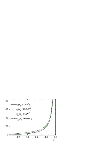
Figure 3: The comparison of the behavior of the saddle point $\displaystyle c_{0}$ and the point $\displaystyle c_{as}$ versus of $\displaystyle x_{\tt B}$ at two fixed values of $\displaystyle Q^{2}$.

Next, from the zero phase condition follows that $\displaystyle\omega_{\tt B}y-\left[(\beta+1)+\Delta(Q^{2})\right]\arg{z}=0\,$. Therefore, the asymptotic behavior of the contour as $\displaystyle{\rm Re}z\to-\infty$ is determined by the formula

$$\displaystyle x_{as}^{{\tt DIS}}(y,Q^{2})=y{\rm ctg}\left[{\frac{\omega_{\tt B}y}{(\beta+1)+\Delta(Q^{2})}}\right]\,.$$ (39)

In the asymptotic region the contour $\displaystyle C_{as}$ tends to the finite limiting value

$$\displaystyle y_{as}^{{\tt DIS}}(Q^{2})=\pm\,\frac{\left[~{}(\beta+1)+\Delta(Q^{2})\right]\pi}{\omega_{\tt B}}\,.$$ (40)

Thus, the account of the $\displaystyle Q^{2}$-evolution of the Mellin moments of the $\displaystyle F_{3}$ structure function comes down to replacement in the expressions without evolution $\displaystyle\beta\Rightarrow\beta+\Delta(Q^{2})$ and using Eq. (35) $\displaystyle x_{as}^{{\tt DIS}}(y)\Rightarrow x_{as}^{{\tt DIS}}(y,Q^{2})$ and $\displaystyle y_{as}^{{\tt DIS}}\Rightarrow y_{as}^{{\tt DIS}}(Q^{2})$.

It is important to note that the expression defining the contour $\displaystyle C_{as}$ in higher orders of the perturbation theory QCD will coincides with the $\displaystyle LO$ expression with the replacement only of $\displaystyle\alpha_{s}^{LO}(Q^{2})$ in Eq. (37) by an expression for the running coupling in the corresponding order of the perturbation theory.

Figure 3 shows the influence of the $\displaystyle Q^{2}$ evolution on a values of the saddle point $\displaystyle c_{0}$ and the ‘asymptotic’ point $\displaystyle~{}c_{as}=x_{as}(y=0)$ in the case of the $\displaystyle F_{3}$ structure function. In this figure $\displaystyle c_{0}$ and $\displaystyle c_{as}$ are shown as functions of the Bjorken variable $\displaystyle x_{\tt B}$ at $\displaystyle Q^{2}=Q^{2}_{0}=3~{}{\rm GeV}^{2}$ (solid and dashed lines for $\displaystyle c_{0}$ and $\displaystyle c_{as}$, respectively) and $\displaystyle Q^{2}=100~{}{\rm GeV}^{2}$ (dotted and dash-dotted lines). One can see that there is no significant difference in the behavior of the point $\displaystyle c_{0}$ with changing of $\displaystyle Q^{2}$ as the solid and dotted curves are close to each other. The same behavior is observed also for the point $\displaystyle c_{as}$. It is interesting to note a sharp increase in the values of $\displaystyle c_{0}$ and $\displaystyle c_{as}$ if $\displaystyle x_{\tt B}>0.5$, as well as the convergence of all curves at large values of $\displaystyle x_{\tt B}$.

V Numerical estimations of accuracy

Table 1: The relative accuracy $\displaystyle\varepsilon(N)$ of numerical evaluation of the MB integral (14) for different values of terms $\displaystyle N$ in the sum (13), when the contour $\displaystyle C_{K}$ is used, and in the sum (23) for the contour $\displaystyle C_{as}$.

	$\displaystyle-s=1/20$		$\displaystyle-s=2.0$
$\displaystyle N$	$\displaystyle C_{K}$	$\displaystyle C_{as}$	$\displaystyle C_{K}$	$\displaystyle C_{as}$
$\displaystyle 16$	$\displaystyle 1.2\times 10^{-8}~{}~{}$	$\displaystyle 1.3\times 10^{-7}$	$\displaystyle~{}~{}~{}1.2\times 10^{-6}$	$\displaystyle~{}6.5\times 10^{-5}$
$\displaystyle 20$	$\displaystyle 6.7\times 10^{-10}$	$\displaystyle~{}8.5\times 10^{-12}$	$\displaystyle~{}~{}~{}4.0\times 10^{-6}$	$\displaystyle~{}3.9\times 10^{-6}$
$\displaystyle 30$	$\displaystyle 1.2\times 10^{-11}$	$\displaystyle~{}5.7\times 10^{-14}$	$\displaystyle~{}~{}~{}5.1\times 10^{-7}$	$\displaystyle~{}1.2\times 10^{-8}$
$\displaystyle 35$	$\displaystyle 5.8\times 10^{-13}$	$\displaystyle~{}5.7\times 10^{-16}$	$\displaystyle~{}~{}~{}1.4\times 10^{-7}$	$\displaystyle~{}5.8\times 10^{-11}$

Table 2: The relative accuracy $\displaystyle\varepsilon(N)$ of the $\displaystyle x_{\tt B}F_{3}(x_{\tt B},Q_{0}^{2})$ reconstruction for different values of terms $\displaystyle N$ in the sums (13) and (35), for the contours $\displaystyle C_{K}$ and $\displaystyle C_{as}$, respectively.

	$\displaystyle x_{\tt B}=0.01$		$\displaystyle x_{\tt B}=0.1$		$\displaystyle x_{\tt B}=0.5$
$\displaystyle N$	$\displaystyle C_{K}$	$\displaystyle C_{as}$	$\displaystyle C_{K}$	$\displaystyle C_{as}$	$\displaystyle C_{K}$	$\displaystyle C_{as}$
$\displaystyle 16$	$\displaystyle 2.5\times 10^{-8}$	$\displaystyle 3.2\times 10^{-7}$	$\displaystyle 1.3\times 10^{-9}$	$\displaystyle 2.9\times 10^{-8}$	$\displaystyle 1.0\times 10^{-13}$	$\displaystyle 1.4\times 10^{-11}$
$\displaystyle 20$	$\displaystyle 3.7\times 10^{-10}$	$\displaystyle 4.1\times 10^{-9}$	$\displaystyle 1.0\times 10^{-10}$	$\displaystyle 1.6\times 10^{-10}$	$\displaystyle 1.8\times 10^{-17}$	$\displaystyle 4.6\times 10^{-15}$
$\displaystyle 30$	$\displaystyle 2.7\times 10^{-11}$	$\displaystyle 7.6\times 10^{-13}$	$\displaystyle 5.7\times 10^{-13}$	$\displaystyle 3.6\times 10^{-16}$	$\displaystyle 3.8\times 10^{-19}$	$\displaystyle 8.7\times 10^{-21}$
$\displaystyle 35$	$\displaystyle 9.7\times 10^{-13}$	$\displaystyle 1.5\times 10^{-16}$	$\displaystyle 5.1\times 10^{-14}$	$\displaystyle 1.5\times 10^{-16}$	$\displaystyle 4.3\times 10^{-20}$	$\displaystyle 3.6\times 10^{-23}$

In this section, by numerically calculating the MB integrals given by Eqs. (14) and (28), we investigate the question at what values of polynomials $\displaystyle N$ in the corresponding quadrature formula the advantages of the asymptotic contour $\displaystyle C_{as}$ are manifested, in comparison with the quadratic approximation $\displaystyle C_{K}$ to the contour of the stationary phase.

The relative accuracy of a reconstruction is defined as usual $\displaystyle\varepsilon(N)=|({f_{N}-f^{exact}})/{f^{exact}}|\,,$ where $\displaystyle f_{N}$ is the sum given by Eq. (13), when the contour $\displaystyle C_{K}$ is used, or Eq. (23) for the contour $\displaystyle C_{as}$; $\displaystyle f^{exact}$ is the exact value of the corresponding integral.

The relative accuracy $\displaystyle\varepsilon(N)$ of calculating the $\displaystyle I(s)$ integral depending on number of terms $\displaystyle N$ in the sums (13) and (23) is presented in Table 1. The result is given for $\displaystyle-s=1/20$ and $\displaystyle-s=2.0$. The calculations for the $\displaystyle F_{3}$ structure function are presented in Table 2 for the values $\displaystyle x_{B}=0.01,~{}0.1$, and $\displaystyle 0.5$. In doing so, we use the values of the parameters in Eq. (26) that were found in Ref. SS-F3-2 at fixed $\displaystyle Q_{0}^{2}=3$ GeV².

Tables 1 and 2 show similar results for the relative accuracy $\displaystyle\varepsilon(N)$. The contour $\displaystyle C_{K}$ works more efficiently for a small the number of terms ($\displaystyle N<20$) in the quadrature formulae (13) and (23), as for a large $\displaystyle N>20$, the result of the asymptotic contour $\displaystyle C_{as}$ is more accurate by 2–3 orders of magnitude. In addition, as can be seen from Table 2, the high accuracy achieved at $\displaystyle N^{\ast}=20$ exceeds the experimental accuracy by several orders of magnitude. However, as can be seen from Table 1, the “regime change“ for the integral $\displaystyle I(-s=2.0)$ occurs at value of $\displaystyle\varepsilon(N^{\ast})\simeq 4\times 10^{-6}$. Such accuracy has practical importance in the QFT calculations.

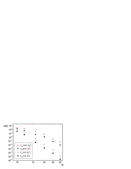
Figure 4: The comparison of the relative accuracy $\displaystyle\varepsilon(N)$ of the $\displaystyle x_{\tt B}F_{3}(x_{\tt B},Q^{2})$ reconstruction versus the number of terms $\displaystyle N$ in the sum (23) at $\displaystyle x_{\tt B}=0.01$ (triangles) and $\displaystyle x_{\tt B}=0.5$ (squares) using the contour $\displaystyle C_{as}(x_{\tt B},Q_{0}^{2})$ (open triangles and squares) and $\displaystyle C_{as}(x_{\tt B},Q^{2})$ (full triangles and squares) for $\displaystyle Q_{0}^{2}=3$ GeV² and $\displaystyle Q^{2}=100$ GeV².

Figure 4 shows the effect of the contour $\displaystyle Q^{2}$ evolution according to Eq. (39) for the $\displaystyle F_{3}$ structure function. In this figure the relative accuracy $\displaystyle\varepsilon(N)$ is plotted as a function of number terms $\displaystyle N$ in the Gauss-Legendre quadrature formula (23) at values of the Bjorken variable $\displaystyle x_{\tt B}=0.01$ (triangles) and $\displaystyle x_{\tt B}=0.8$ (squares) for the contours $\displaystyle C_{as}(x_{\tt B},Q_{0}^{2})$ (open triangles and squares) and $\displaystyle C_{as}(x_{\tt B},Q^{2})$ (full triangles and squares) for $\displaystyle Q^{2}=Q_{0}^{2}=3$ GeV² and $\displaystyle Q^{2}=100$ GeV². For the running coupling $\displaystyle\alpha_{s}^{LO}(Q^{2})$ we used a value $\displaystyle\Lambda_{{\rm QCD}}=363$ MeV and $\displaystyle n_{f}=4$ (see Ref. SS-F3-2 ). One can see that the contour $\displaystyle C_{as}(x_{\tt B},Q^{2})$ yields a more exact result; however, this advantage is compensated when using the contour $\displaystyle C_{as}(Q^{2}_{0})$ if the number of terms $\displaystyle N$ is increased by 2–4 units.

VI Conclusions

We presented a new approximation for the construction of a contour close to the contour of the stationary phase. A special case of the finite asymptotics of the stationary-phase contour in the limit $\displaystyle{\rm Re}z\to-\infty$ was considered as such an asymptotics arises in the calculation of the MB integral that represents the $\displaystyle F_{3}$ structure function in terms of its Mellin moments. The proposed approximation reproduces the behavior of the contour zero phase for large values of $\displaystyle|z|$ and has the form like Eq. (34) in the case of the DIS structure functions.

It was compared the efficiency of application of the asymptotic stationary phase contour $\displaystyle C_{as}$ and the contour $\displaystyle C_{K}$, determined by the saddle-point method, as described in Sec. II, in calculating of the MB integrals (14) and (28). As expected, the contour $\displaystyle C_{K}$ turned out to be more effective for a small number of $\displaystyle N$ terms in the Gauss–Laguerre quadrature formula, when the nodes of the quadrature formulas are located near the saddle point Kosower:1997hg ; Sidorov:2017 . The advantage of the contour $\displaystyle C_{as}$ is manifested at large values of $\displaystyle N$. The “regime change“ occurs at $\displaystyle N^{\ast}\approx 20$. For the region $\displaystyle 20<N\leqslant 35$, the contour $\displaystyle C_{as}$ gives a relative error of 2–3 orders of magnitude better than the contour $\displaystyle C_{K}$. With increasing $\displaystyle N$, this gap increases too.

When the $\displaystyle Q^{2}$-evolution of the structure function $\displaystyle F_{3}$ is taken into account, the efficiency of the contours $\displaystyle C_{as}{(Q_{0}^{2})}$ and $\displaystyle C_{as}{(Q^{2})}$ was compared. Although the contour $\displaystyle C_{as}{(Q^{2})}$ gives a more accurate result, but this advantage is compensated by using the contour $\displaystyle C_{as}{(Q_{0}^{2})}$ if we increase the number of terms in the quadrature formula only by 2–3 units. The contour $\displaystyle C_{as}{(Q_{0}^{2})}$ can be considered as a universal one, that is, applicable for other values of $\displaystyle Q^{2}$.

It should be emphasized that since the necessary accuracy is achieved when using a small number of $\displaystyle N$ in the quadrature formulas (13) or (21), the computer time for calculating the $\displaystyle F_{3}$ structure function by using Eq. (28) with the efficient contours is significantly less than if one uses the linear contours that are usually parallel to the imaginary axis, to the right of the rightmost pole in the integrand, or a straight line at an angle (see, e.g., Refs. Gluck:1989ze ; Graudenz:1995sk ; deFlorian:2017lwf ; Leader:2015hna ).

Here we have considered the $\displaystyle F_{3}$ structure function, which is the simplest among the DIS structure functions since it does not contain the contribution of gluons and sea quarks. The parameterization of the shape of this structure function (26) is typical and widely used in the QCD analysis of the structure functions. Our consideration can be applied to the polarized nonsinglet combination $\displaystyle\Delta q_{3}$, $\displaystyle\Delta q_{8}$ and the nonsinglet combination fragmentation function $\displaystyle D^{\pi^{+}}_{u_{v}}$. The choice of the efficient contour for the singlet case can be performed along the same line, but requires more complicated formulas. This is the task for forthcoming investigation.

Our result can be useful in choosing an integration method in both the one-dimensional case and the case of few-dimensional MB integrals if it is required to achieve relative accuracy unattainable in the integration by the Monte Carlo method.

Appendix A On numerical evaluation of $\displaystyle I(s)$ for $\displaystyle-s>4$

Let us turn to the MB integral (14) and a little discuss the efficient contours for the case $\displaystyle-s>4$. The exact result is written as follows

$$\displaystyle~{}~{}I(s)=2\ln(-s) \displaystyle- \displaystyle s\left(1-\sqrt{1+\frac{4}{s}}\right)$$

$$\displaystyle+ \displaystyle 4\ln\left[\frac{1}{2}+\frac{1}{2}\sqrt{1+\frac{4}{s}}\right]\,,~{}-s>4\,.$$

Figure 5: The comparison of the efficient contours for the MB integral (14) in the region $\displaystyle-s>4$. The notations are the same as in Fig. 1.

This case is interesting for us, because the exact contour of zero phase $\displaystyle C_{st}$, see Eq. (25), go away from the imaginary axis to the right. The asymptotic behavior of the contour $\displaystyle C_{st}$ is defined by Eq. (18), as before, however, from this equation it follows that in the asymptotic region as $\displaystyle{\rm Re}z\to+\infty$ the contour tends to another limit value

$$\displaystyle y_{as}=\,\frac{3}{2}\frac{~{}\pi}{|\omega+\ln 4|}\;{\rm sign}(y)\,.$$ (42)

Therefore, the numerical value of the integral $\displaystyle I(s)$ can be found using the Gauss–Legendre quadrature formula (23) in which $\displaystyle y_{as}$ is given by Eq. (42) and the contour $\displaystyle C_{as}$ by Eqs. (18) and(24).

The contours $\displaystyle C_{K}$ and $\displaystyle\overline{C}_{K}$ are defined by the same way as before, and the numerical value of the integral $\displaystyle I(s)$ is determined using the Gauss–Laguerre quadrature formula (13).

Figure 5 shows the shape of contours for fixed $\displaystyle-s=5$. The solid curve corresponds to the contour $\displaystyle C_{as}$, the dotted curve is the exact contour $\displaystyle C_{st}$, the dashed curve is the contour $\displaystyle C_{K}$, and the dash-dotted is the contour $\displaystyle\overline{C}_{K}$. From this figure it is clear that in calculating the integral $\displaystyle I(s)$ using the contour $\displaystyle{C}_{K}$, difficulties will arise, as this contour has an incorrect direction. Only the first few terms in the sum (13) may give a reasonable result, since the contour $\displaystyle C_{K}$ is close to the contour $\displaystyle C_{st}$ near the saddle point $\displaystyle c_{0}$. Thus, for the case $\displaystyle-s>4$ the contour $\displaystyle C_{K}$ it is impossible to consider as efficient. At the same time, the contour $\displaystyle\overline{C}_{K}$ works rather good, but applying it to achieve relative accuracy, for example, $\displaystyle 10^{-12}$, can be problematic. The proposed contour $\displaystyle C_{as}$, whose a construction is quite simple, reproduces the behavior of the exact contour $\displaystyle C_{st}$ well, and the use of this contour can provide the required high relative accuracy.

References

• (1) H. Bateman and A. Erdelyi, Higher transcendental functions, Vol. 1, New York (McGraw-Hill, 1953).
• (2) J. Gluza, T. Jelinski, and D. A. Kosower, Phys. Rev. D 95, 076016 (2017).
• (3) M. Gl$\displaystyle\ddot{{\rm u}}$ck and E. Reya, Phys. Rev. D 14, 3034 (1976).
• (4) M. Gl$\displaystyle\ddot{{\rm u}}$ck, E. Reya, and A. Vogt, Z. Phys. C 48, 471 (1990).
• (5) D. Graudenz, M. Hampel, A. Vogt, and C. Berger, Z. Phys. C 70, 77 (1996).
• (6) I. Dubovyk, J. Gluza, T. Jelinski, T. Riemann, and J. Usovitsch, Acta Phys. Polon. B 48, 995 (2017).
• (7) D. A. Kosower, Nucl. Phys. B 506, 439 (1997).
• (8) V. I. Lashkevich, A. V. Sidorov, and O. P. Solovtsova, Nonlin. Phenom. Complex Syst.  20, 286 (2017).
• (9) P. Rabinowitz and G. Weiss, Math. Comp. 13, 285 (1959).
• (10) A. V. Sidorov and O. P. Solovtsova, Mod. Phys. Lett. A 29, 1450194 (2014).
• (11) A. J. Buras, Rev. Mod. Phys. 52, 199 (1980).
• (12) D. de Florian, M. Epele, R. J. Hernandez-Pinto, R. Sassot, and M. Stratmann, Phys. Rev. D 95, 094019 (2017).
• (13) E. Leader, A. V. Sidorov, and D. B. Stamenov, Phys. Rev. D 93, 074026 (2016).