Influence of the SIPG penalisation on the numerical properties of linear systems for elastic wave propagation

Abstract

Interior penalty discontinuous Galerkin discretisations (IPDG) and especially the symmetric variant (SIPG) for time-domain wave propagation problems are broadly accepted and widely used due to their advantageous properties. Linear systems with block structure arise by applying space-time discretisations and reducing the global system to time-slab problems. The design of efficient and robust iterative solvers for linear systems from interior penalty discretisations for hyperbolic wave equations is still a challenging task and relies on understanding the properties of the systems. In this work the numerical properties such as the condition number and the distribution of eigenvalues of different representations of the linear systems coming from space-time discretisations for elastic wave propagation are numerically studied. These properties for interior penalty discretisations depend on the penalisation and on the time interval length.

1 Introduction

The accurate and efficient simulation of time-domain first- and second-order hyperbolic elastic and acoustic wave propagation phenomena is of importance in many engineering fields with e.g. electromagnetic, acoustic and seismic applications as well as for non-destructive structural health monitoring of light-weighted fibre reinforced materials; cf. e.g. [1, 2] and references therein. Recently there is again an increased interest in the simulation of multi-physics systems including coupled elastic wave propagation together with fluid flow in porous media; cf. [3, 4]. Such models appear for instance in battery engineering and for biomedical applications.

The ability of the efficient high-order approximation of the space-time wavefield is of fundamental importance for time-domain numerical simulations of wave phenomena. Especially discontinuous Galerkin methods (dG) as spatial discretisations exhibit as favourable over continuous finite element methods in terms of lesser numerical dispersion at the same discretisation order such as polynomial degree and degrees of freedom per wavelength; cf. [5]. Reed and Hill introduced in 1973 the first discontinuous Galerkin method for first-order hyperbolic steady-state neutron transport. Meanwhile there exist many discontinuous Galerkin methods for the spatial discretisation of elliptic, parabolic and hyperbolic problems; cf. e.g. [8].

Interior penalty discontinuous Galerkin discretisations (IPDG) and especially the symmetric interior penalty variant (SIPG) for time-domain wave propagation problems are broadly accepted and widely used due to their advantageous properties and their ability for parallel numerical simulations. The SIPG discretisation of the second-order wave equations is convergent of optimal order in the energy- and $L^{2}$-norm for any polynomial approximation degree in space; cf. [7]. All interior penalty discontinuous Galerkin families include additional terms combined of trace operators on the interior and exterior boundaries between mesh elements. Interior penalty methods include a stabilisation term which penalises jumps of the trial and test function traces on the boundaries to ensure coercivity of the bilinear form corresponding to the Laplacian operator. The needed weighting depends on spatial mesh parameters such as the cell diameter, the cell anisotropy and the local polynomial degree as well as on material parameters but not on the time discretisation parameters; cf. [6, 7, 8]. The estimation of the local minimal choice of the penalisation is of fundamental importance but it turns out to be difficult in physically relevant problems. An over-penalisation should be avoided since such results in linear systems with higher condition numbers than necessary. The over-penalisation may result in inefficient iterative system solves or breakdowns if it is not take into account in the solver design.

The common drawback of discontinuous Galerkin discretisations compared to their continuous Galerkin counterparts is that they need more degrees of freedom to obtain the same analytic convergence order. In physically relevant problems the drawback of the higher number of degrees of freedom is not that present compared to analytic test problems. To the contrary, physically relevant problems gain advantages, such as avoiding linear-elasticity locking phenomena and the ability to capture incompatible but relevant boundary and initial conditions, from the lesser grid stiffness of discontinuous approaches in space and time; cf. e.g. [1].

Linear systems with block structure arise by applying space-time discretisations and reducing the global system to time-slab or time-interval problems; cf. [1]. The design of efficient and robust iterative solvers for linear systems from interior penalty discretisations for hyperbolic wave equations is still a challenging task and relies on understanding the properties of the systems.

This work presents the numerical properties such as the condition number and the distribution of eigenvalues and their dependency on the penalisation and on the time interval length of different representations of the linear systems coming from space-time discretisations for elastic wave propagation. To the best knowledge of the author such results are not present in the literature.

The following structure of the paper is the brief introduction of the elastic wave equation and its space-time discretisation in Sec. 2, the presentation of different representations of the fully discrete systems which are further studied in Sec. 3, the numerical experiments section providing the results in Sec. 4 and summarising and concluding remarks in Sec. 5.

2 Elastic wave equation and space-time discretisation

The elastic wave equation in its first-order in time, or displacement-velocity, representation reads as the following system. The primal variables are the displacement $\boldsymbol{u}$ and the velocity $\boldsymbol{v}$. The volume is represented by the domain $\Omega\subset\mathbb{R}^{d}$, with dimension $d=2,3$, and the time domain is given by $I=(0,T)$ for some finite final time $T$. Find the pair $\{\boldsymbol{u},\boldsymbol{v}\}$ from

$$\begin{array}[]{r@{\,}c@{\,}l@{\;}c@{\;}l@{\quad}l}\rho_{s}(\boldsymbol{x})\partial_{t}\boldsymbol{u}(\boldsymbol{x},t)&-&\rho_{s}(\boldsymbol{x})\boldsymbol{v}(\boldsymbol{x},t)&=&\boldsymbol{0}&\text{in }\;\Omega\times I\,,\\[6.45831pt] \rho_{s}(\boldsymbol{x})\partial_{t}\boldsymbol{v}(\boldsymbol{x},t)&-&\nabla\cdot\boldsymbol{\sigma}(\boldsymbol{u}(\boldsymbol{x},t))&=&\boldsymbol{f}(\boldsymbol{x},t)&\text{in }\;\Omega\times I\,,\end{array}$$ (1)

with boundary conditions $\boldsymbol{u}(\boldsymbol{x},t)=\boldsymbol{g}(\boldsymbol{x},t)$ on $\Gamma_{D}\times I$, $\boldsymbol{\sigma}(\boldsymbol{u}(\boldsymbol{x},t))\,\boldsymbol{n}=\boldsymbol{h}(\boldsymbol{x},t)$ on $\Gamma_{N}\times I$, and initial conditions $\boldsymbol{u}(\boldsymbol{x},0)=\boldsymbol{u}_{0}(\boldsymbol{x})$ in $\Omega\times\{0\}$, $\boldsymbol{v}(\boldsymbol{x},0)=\boldsymbol{v}_{0}(\boldsymbol{x})$ in $\Omega\times\{0\}$. The linearised stress tensor is given by $\boldsymbol{\sigma}(\boldsymbol{u})=\boldsymbol{C}:\boldsymbol{\epsilon}(\boldsymbol{u})$ and is composed of the action of the (possibly anisotropic) linear elasticity tensor $\boldsymbol{C}$ on the linearised strain $\boldsymbol{\epsilon}(\boldsymbol{u})=(\nabla\boldsymbol{u}+\nabla\boldsymbol{u}^{T})/2$. The solid mass densities inside the volume are denoted by $\rho_{s}$. Acting internal volume forces are denoted by $\boldsymbol{f}$. A detailed derivation of the system can be found in [1].

Standard notation for function spaces, norms and inner products is used. Let $\boldsymbol{H}=L^{2}(\Omega)^{d}$, $\boldsymbol{V}=H^{1}_{0}(\Gamma_{D};\Omega)^{d}$, $\boldsymbol{V}^{*}=H^{-1}(\Gamma_{D};\Omega)^{d}$, $\mathcal{H}=L^{2}(I;\boldsymbol{H})$, $\mathcal{V}=\{\boldsymbol{v}\in L^{2}(I;\boldsymbol{V})\,|\,\partial_{t}\boldsymbol{v}\in\mathcal{H}\}$ and $\mathcal{W}=L^{2}(I;\boldsymbol{V})$. The initial-boundary value problem with purely homogeneous Dirichlet boundary condition $\boldsymbol{g}=\boldsymbol{0}$ admits an unique weak solution $\boldsymbol{u}\in\mathcal{V}\cap C(\widebar{I};\boldsymbol{V})$, $\boldsymbol{v}\in\mathcal{H}\cap C(\widebar{I};\boldsymbol{H})$ and $\partial_{t}\boldsymbol{v}\in L^{2}(I;\boldsymbol{V}^{*})$ as given by the literature.

A variational space-time discretisation is briefly presented in the sequel; for all details consider [1]. A piecewise polynomial continuous Galerkin approximation of polynomial degree $r$ is used as semi-discretisation in time. Hereby a piecewise discontinuous space of polynomial degree $r-1$ is used as test function space which allows the truncation of the global space-time system to time interval or time slab problems. Let $0=t_{0}<\dots<t_{N}=T$ the partition of the temporal domain $I=(0,T)$ into $N$ subintervals $I_{n}=(t_{n-1},t_{n})$, $n=1,\dots,N$. The length of the subinterval $I_{n}$ is defined by $\tau_{n}=t_{n}-t_{n-1}$ and let $\tau=\max_{1\leq n\leq N}\tau_{n}$ the global time discretisation parameter. Let $\mathbb{P}_{r}(I_{n};X)$ denote the space of polynomials of degree $r$ or less on the interval $I_{n}\subset I$ with values in some Banach space $X$. Introducing $\xi\in C(\widebar{I};\mathbb{R})$, with $\xi|_{I_{n}}\in\mathbb{P}_{r}(\widebar{I}_{n};\mathbb{R})$, and $\zeta\in L^{2}(I;\mathbb{R})$, with $\zeta|_{I_{n}}\in\mathbb{P}_{r}(\widebar{I}_{n};\mathbb{R})$, as global piecewise polynomial trail and test basis functions. The semi-discrete system reads as: Find the pairs $\{{\boldsymbol{u}}_{\tau}^{\textnormal{cG}}|_{I_{n}},{\boldsymbol{v}}_{\tau}^{\textnormal{cG}}|_{I_{n}}\}\in\mathbb{P}_{r}(I_{n};\boldsymbol{V})\times\mathbb{P}_{r}(I_{n};\boldsymbol{V})$, with coefficients ${\boldsymbol{U}}_{n}^{\iota},{\boldsymbol{V}}_{n}^{\iota}\in\boldsymbol{V}$ for $\iota=1,\dots,r$, such that

$$\begin{array}[]{l@{\,}c@{\,}r@{\,}c@{\,}l@{\quad}l}\displaystyle\sum_{\iota=0}^{r}\Big{\{}\alpha_{\kappa,\iota}\,(\rho_{s}\,{\boldsymbol{U}}_{n}^{\iota},\widetilde{\boldsymbol{\omega}})&-&\beta_{\kappa,\iota}\,(\rho_{s}\,{\boldsymbol{V}}_{n}^{\iota},\widetilde{\boldsymbol{\omega}})\Big{\}}&=&\boldsymbol{0}\,,&\forall\widetilde{\boldsymbol{\omega}}\in\boldsymbol{V}\,,\\[6.45831pt] \displaystyle\sum_{\iota=0}^{r}\Big{\{}\alpha_{\kappa,\iota}\,(\rho_{s}\,{\boldsymbol{V}}_{n}^{\iota},\widehat{\boldsymbol{\omega}})&+&\beta_{\kappa,\iota}\,a({\boldsymbol{U}}_{n}^{\iota},\widehat{\boldsymbol{\omega}})\Big{\}}&=&\displaystyle\sum_{\iota=0}^{r}\beta_{\kappa,\iota}\,({\boldsymbol{F}}_{n}^{\iota},\widehat{\boldsymbol{\omega}})\,,&\forall\widehat{\boldsymbol{\omega}}\in\boldsymbol{V}\,,\end{array}$$ (2)

for all $\kappa=1,\dots,r$, and with

$$\begin{array}[]{r@{\,}c@{\,}l@{\,}c@{\,}l@{\,}c@{\,}l}\alpha_{\kappa,\iota}&:=&(\xi_{n,\iota}^{\prime}(t),\zeta_{n,\kappa}(t))_{I_{n}}&=&\displaystyle\int_{\widehat{I}}\widehat{\xi}_{\iota}^{\prime}(\widehat{t})\,\widehat{\zeta}_{\kappa}(\widehat{t})\,\mathrm{d}\widehat{t}&=&\displaystyle\sum_{\mu=0}^{r}\widehat{w}_{\mu}\,\widehat{\xi}_{\iota}^{\prime}(\widehat{t}_{\mu})\,\widehat{\zeta}_{\kappa}(\widehat{t}_{\mu})\,,\\[6.45831pt] \beta_{\kappa,\iota}&:=&(\xi_{n,\iota}(t),\zeta_{n,\kappa}(t))_{I_{n}}&=&\displaystyle\int_{\widehat{I}}\widehat{\xi}_{\iota}(\widehat{t})\,\widehat{\zeta}_{\kappa}(\widehat{t})\,\tau_{n}\,\mathrm{d}\widehat{t}&=&\displaystyle\sum_{\mu=0}^{r}\tau_{n}\,\widehat{w}_{\mu}\,\widehat{\xi}_{\iota}(\widehat{t}_{\mu})\,\widehat{\zeta}_{\kappa}(\widehat{t}_{\mu})\,,\end{array}$$ (3)

using quadrature weights $\widehat{w}_{\mu}$ and quadrature points $\widehat{t}_{\mu}$ from $\widehat{\mathcal{Q}}_{\text{GL($r$+1)}}$ such that the continuity conditions between neighbouring subintervals hold.

For the discretisation in space, let the partition $\mathcal{T}_{h}$ of the space domain $\Omega$ into some finite number of disjoint elements $K$. Denoting by $h_{K}$ the diameter of the element $K$ and the global space discretisation parameter as $h=\max_{K\in\mathcal{T}_{h}}h_{K}$. The spatial mesh is allowed to be anisotropic but non-degenerated. Let the partition $\widebar{\mathcal{F}}_{h}=\widebar{\mathcal{F}}_{h}^{\mathcal{B}}\cup\mathcal{F}_{h}^{\mathcal{I}}$ into disjoint parts $\widebar{\mathcal{F}}_{h}^{\mathcal{B}}$, $\mathcal{F}_{h}^{\mathcal{I}}$ for the set of boundary faces and the set of interior faces. The set of boundary faces is divided as $\widebar{\mathcal{F}}_{h}^{\mathcal{B}}:=\mathcal{F}_{h}^{\mathcal{B}(\Gamma_{D})}\cup\mathcal{F}_{h}^{\mathcal{B}(\Gamma_{N})}$, $\mathcal{F}_{h}^{\mathcal{B}}:=\mathcal{F}_{h}^{\mathcal{B}(\Gamma_{D})}$, into disjoint parts $\mathcal{F}_{h}^{\mathcal{B}(\Gamma_{D})}$, $\mathcal{F}_{h}^{\mathcal{B}(\Gamma_{N})}$ coinciding with the Dirichlet boundary $\Gamma_{D}$ and the Neumann boundary $\Gamma_{N}$. We let $\mathcal{F}_{h}:=\mathcal{F}_{h}^{\mathcal{B}(\Gamma_{D})}\cup\mathcal{F}_{h}^{\mathcal{I}}=\mathcal{F}_{h}^{\mathcal{B}}\cup\mathcal{F}_{h}^{\mathcal{I}}$. The jump trace operators, which enforce weak Dirichlet boundary conditions, are defined by

$$\begin{array}[]{r @{\quad} r}\llbracket\boldsymbol{v}\rrbracket_{0}:=\begin{cases}\boldsymbol{v}|_{F^{+}}-\boldsymbol{v}|_{F^{-}}\,,&F\in\mathcal{F}_{h}^{\mathcal{I}}\,,\\[2.15277pt] \boldsymbol{v}|_{F^{+}}\,,&F\in\mathcal{F}_{h}^{\mathcal{B}}\,,\end{cases}&\llbracket\boldsymbol{v}\rrbracket:=\begin{cases}\boldsymbol{v}|_{F^{+}}-\boldsymbol{v}|_{F^{-}}\,,&F\in\mathcal{F}_{h}^{\mathcal{I}}\,,\\[2.15277pt] \boldsymbol{v}|_{F^{+}}-\boldsymbol{v}|_{\Gamma_{D}}\,,&F\in\mathcal{F}_{h}^{\mathcal{B}}\,.\end{cases}\end{array}$$ (4)

The average trace operator is defined by

$$\{\{{\boldsymbol{t}}_{F}(\boldsymbol{v})\}\}:=\begin{cases}\frac{1}{2}\big{(}{\boldsymbol{t}}_{F}\big{(}\boldsymbol{v}|_{F^{+}}\big{)}+{\boldsymbol{t}}_{F}\big{(}\boldsymbol{v}|_{F^{-}}\big{)}\big{)}\,,&F\in\mathcal{F}_{h}^{\mathcal{I}}\,,\\[2.15277pt] {\boldsymbol{t}}_{F}\big{(}\boldsymbol{v}|_{F^{+}}\big{)}\,,&F\in\mathcal{F}_{h}^{\mathcal{B}}\,,\end{cases}$$ (5)

using the traction vector ${\boldsymbol{t}}_{F}\big{(}\boldsymbol{v}|_{F^{\pm}}\big{)}:={\boldsymbol{\sigma}}\big{(}\boldsymbol{v}|_{F^{\pm}}\big{)}\boldsymbol{n}^{\pm}$.

To be concise as possible, we give directly the bilinear form $a_{h}$ corresponding to the weak Laplacian as

$$\begin{array}[]{r@{\,}c@{\,}l}a_{h}({\boldsymbol{u}}_{h}^{n,\iota},\boldsymbol{\omega}_{h})&=&\displaystyle\sum_{K\in\mathcal{T}_{h}}\int_{K}{\boldsymbol{\sigma}}({\boldsymbol{u}}_{h}^{n,\iota}):{\boldsymbol{\epsilon}}(\boldsymbol{\omega}_{h})-\displaystyle\sum_{F\in\mathcal{F}_{h}}\int_{F}\{\{{\boldsymbol{t}}_{F}({\boldsymbol{u}}_{h}^{n,\iota})\}\}\cdot\llbracket\boldsymbol{\omega}_{h}\rrbracket_{0}\\[6.45831pt] &{}\hfil&+\displaystyle\sum_{F\in\mathcal{F}_{h}}\int_{F}\llbracket{\boldsymbol{u}}_{h}^{n,\iota}\rrbracket\cdot\Big{(}\gamma_{F}\,\llbracket\boldsymbol{\omega}_{h}\rrbracket_{0}-S\,\{\{{\boldsymbol{t}}_{F}(\boldsymbol{\omega}_{h})\}\}\Big{)}\,,\end{array}$$ (6)

where $S\in\{1,-1,0\}$ denotes the consistency parameter. The choice $S=1$ leads to SIPG, $S=-1$ to NIPG and $S=0$ to IIPG. Note that the non-homogeneous Dirichlet boundary terms can be shifted efficiently to the right hand side and thus only a stiffness matrix for homogeneous Dirichlet boundaries has to be assembled. The value of the interior penalty parameter $\gamma_{F}$ is determined by an inverse estimate to balance the terms involving numerical fluxes on the element boundaries $F\in\mathcal{F}_{h}$ in Eq. (6) and to ensure coercivity of the bilinear form $a_{h}$. We let $\gamma_{F}=\gamma_{0}\,\gamma_{F,{\boldsymbol{C}}}\,\gamma_{F,K}$, where $\gamma_{F,K}$ denotes a parameter depending only the polynomial approximation degree $p$ in space and the shape of the elements $K^{\pm}$, $\gamma_{F,{\boldsymbol{C}}}$ denotes a (scalar) parameter depending the material parameters in $K^{\pm}$ and $\gamma_{0}$ denotes an additional tuning parameter; cf. for details [1, 6].

3 Fully discrete systems

In this work only the linear systems of continuous piecewise linear approximations in time, that are SIPG($p$)–cG($1$) and FEM($p$)–cG($1$), are studied. The results can be used for higher order time discretisations, since their efficiency depends strongly on solving additional problems corresponding to the following systems; cf. for details [1].

To derive fully discrete systems from Eq. (2), the basis functions in time are specified as Lagrange polynomials, which are defined via the quadrature points $\widehat{t}_{0}=0$ and $\widehat{t}_{1}=1$ of the two-point Gauß-Lobatto quadrature rule $\widehat{\mathcal{Q}}_{\text{GL($2$)}}$ on the time reference interval $\widehat{I}=[0,1]$.

$$\begin{array}[]{l@{\,}c@{\,}l@{\quad}l@{\,}c@{\,}l@{\quad\quad\quad}l@{\,}c@{\,}l}\widehat{\xi}_{0}(\widehat{t})&=&1-\widehat{t}\,,&\widehat{\xi}_{0}^{\prime}(\widehat{t})&=&-1\,,\\[6.45831pt] \widehat{\xi}_{1}(\widehat{t})&=&\widehat{t}\,,&\widehat{\xi}_{1}^{\prime}(\widehat{t})&=&1\,,&\widehat{\zeta}_{1}(\widehat{t})&=&1\,,\end{array}$$

and, with that, the coefficients $\alpha_{\kappa,\iota}$ and $\beta_{\kappa,\iota}$ from Eq. (3) are evaluated as

$$\begin{array}[]{l@{\,}c@{\,}l@{\quad}l@{\,}c@{\,}l}\alpha_{1,0}&=&-1\,,&\alpha_{1,1}&=&1\,,\end{array}\quad\quad\quad\begin{array}[]{l@{\,}c@{\,}l@{\quad}l@{\,}c@{\,}l}\beta_{1,0}&=&\frac{\tau_{n}}{2}\,,&\beta_{1,1}&=&\frac{\tau_{n}}{2}\,.\end{array}$$

We recast the arising algebraic system by the following linear system with block structure: Find the coefficient vectors ${\boldsymbol{u}}_{I_{n}}^{1},{\boldsymbol{v}}_{I_{n}}^{1}\in\mathbb{R}^{N_{\textnormal{DoF}}}$ from $\boldsymbol{L}\,\boldsymbol{x}=\boldsymbol{b}$ given by

$$\left[\!\!\begin{array}[]{r@{\;}r}-\frac{\tau_{n}}{2}\boldsymbol{M}&\boldsymbol{M}\\[6.45831pt] \boldsymbol{M}&\frac{\tau_{n}}{2}\boldsymbol{A}\end{array}\!\!\right]\left[\!\!\begin{array}[]{c}{\boldsymbol{v}}_{I_{n}}^{1}\\[6.45831pt] {\boldsymbol{u}}_{I_{n}}^{1}\end{array}\!\!\right]=\left[\!\!\begin{array}[]{c}\boldsymbol{0}\\[6.45831pt] \frac{\tau_{n}}{2}({\boldsymbol{b}}_{I_{n}}^{0}+{\boldsymbol{b}}_{I_{n}}^{1})\end{array}\!\!\right]+\left[\!\!\begin{array}[]{r@{\;}r}\frac{\tau_{n}}{2}\boldsymbol{M}&\boldsymbol{M}\\[6.45831pt] \boldsymbol{M}&-\frac{\tau_{n}}{2}\boldsymbol{A}\end{array}\!\!\right]\left[\!\!\begin{array}[]{c}{\boldsymbol{v}}_{I_{n}}^{0}\\[6.45831pt] {\boldsymbol{u}}_{I_{n}}^{0}\end{array}\!\!\right]\,,$$ (7)

and denoting by $\boldsymbol{M}$ the mass matrix and by $\boldsymbol{A}$ the stiffness matrix. The assemblies ${\boldsymbol{b}}_{I_{n}}^{0}$ and ${\boldsymbol{b}}_{I_{n}}^{1}$ include the contributions from the forcing terms and inhomogeneous Dirichlet boundary from Eq. (6) using Eq. (4).

The flexible GMRES method with an inexact Krylov-preconditioner can be used for example to solve the linear system (7) efficiently. With some algebraic steps, the block system can be condensed to $\boldsymbol{K}\,{\boldsymbol{u}}_{I_{n}}^{1}=\widetilde{\boldsymbol{b}}$ and a postprocessing as given by

$$\begin{array}[]{r@{\,}c@{\,}l}(\boldsymbol{M}+\frac{\tau_{n}^{2}}{4}\boldsymbol{A})\,{\boldsymbol{u}}_{I_{n}}^{1}&=&\frac{\tau_{n}^{2}}{4}({\boldsymbol{b}}_{I_{n}}^{0}+{\boldsymbol{b}}_{I_{n}}^{1})+(\boldsymbol{M}-\frac{\tau_{n}^{2}}{4}\boldsymbol{A}){\boldsymbol{u}}_{I_{n}}^{0}+\tau_{n}\boldsymbol{M}{\boldsymbol{v}}_{I_{n}}^{0}\,,\\[6.45831pt] {\boldsymbol{v}}_{I_{n}}^{1}&=&\frac{2}{\tau_{n}}({\boldsymbol{u}}_{I_{n}}^{1}-{\boldsymbol{u}}_{I_{n}}^{0})-{\boldsymbol{v}}_{I_{n}}^{0}\,.\end{array}$$ (8)

The linear system Eq. (8) is comparable to a classical discretisation by employing a Crank-Nicolson scheme for the time discretisation. Hence, optimised solvers for linear systems with the matrix $\boldsymbol{K}$ can be re-used.

4 Numerical Experiments

In this section we study some numerical properties of the linear systems as of Eq. (8) and Eq. (7). Therefore we approximate the analytic solution

$$\boldsymbol{u}^{E}([x_{1},x_{2}]^{T},t)=\left[\begin{array}[]{c}\sin((t+x_{1})\cdot 2\pi)\\[4.30554pt] \sin((t+x_{2})\cdot 2\pi)\\ \end{array}\right]$$ (9)

on $\Omega\times I=(0,1)^{2}\times(0,1)$ with $\partial\Omega=\Gamma_{D}$. The right hand side, initial and boundary values are derived by plugging $\boldsymbol{u}^{E}$ into Eq. (1). The global mesh size is $h=10^{-1}/(2\sqrt{2})$ and we use $p=2$ elements in space. The material is isotropic with Young’s E modulus $E=70$, Poisson’s ratio $\nu=0.34$ and density $\rho_{s}=2.8$. The numerical simulations are done with the DTM++/ewave frontend solver of the author for the deal.II library; cf. [1].

The solutions of the displacement and velocity are illustrated by Fig. 1. The convergence for the error $\boldsymbol{e}_{\boldsymbol{u}}=\boldsymbol{u}^{E}-{\boldsymbol{u}}_{\tau,h}^{\textnormal{cG(1)}}$ and the dependency on the penalisation $\gamma_{0}$ to obtain a certain accuracy is presented in Fig. 2. For a penalty value of $\gamma_{0}=10^{6}$ the experimental order of convergence in time is $2.00$ in the $L^{2}(I;L^{2}(\Omega))$-norm and the calculated errors of the SIPG and FEM discretisations are comparable. Fig. 3 presents the effects of the penalisation and the time step length $\tau_{n}$ on the condition numbers. Fig. 4 illustrates the distribution of the normalised eigenvalues of the matrix $\boldsymbol{K}$ for SIPG($2$)–cG($1$) with $\gamma_{0}=10^{6}$ for several values of $\tau_{n}$ and the normalised eigenvalues of the matrix $\boldsymbol{K}$ for FEM($2$)–cG($1$) for $\tau_{n}=10^{-6}$.

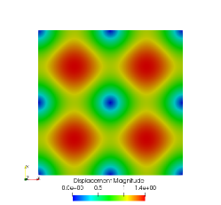
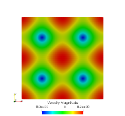
Figure 1: Visualisation of the solution Eq. (9) at $t=1$ for the magnitude of displacement (left) and the velocity (right) with SIPG($2$)–cG($1$) and $\tau_{n}=1.25\cdot 10^{-2}$.

Figure 2: Interior penalty parameter $\gamma_{F}$ influence on the experimental convergence behaviour in time for approximating $\boldsymbol{u}^{E}$ from Eq. (9) for Sec. 4.

Figure 3: Influence of the interior penalty parameter $\gamma_{F}$ and the global time discretisation parameter $\tau_{n}$ on the experimental condition number for Sec. 4.

Figure 4: Distribution of normalised eigenvalues of matrices $\boldsymbol{K}(\tau_{n})$ for SIPG($2$) with $\gamma_{0}=10^{6}$ (solid blue) and for FEM($2$) with $\tau_{n}=10^{-6}$ (dotted red) for Sec. 4.

5 Conclusions

The influence of the penalisation of the SIPG discretisation is analysed numerically for fully discrete linear systems of different representations and compared with their standard finite element counterparts. It is shown that the condition number of the condensed SIPG system matrix scales with the penalisation and the time subinterval length $\tau_{n}$ with a challenging numerical experiment. The eigenvalues collects in small number of clusters for SIPG discretisations by choosing $\tau_{n}\approx 1/\gamma_{0}$. The effect of clustering of the eigenvalues could not be reproduced for the comparable FEM system or for the block system with SIPG. A (much) faster convergence behaviour of the conjugate gradient method for the condensed SIPG system for small time step sizes was noticed but not analysed by the author in the past for several three dimensional problems with physically relevance; cf. [1]. With the results of this work, a faster convergence behaviour of the conjugate gradient method can be explained due to the clustering effect of the eigenvalues in such cases. The results of this work clearly help to design preconditioners for the block system or the condensed system for SIPG discretisations for the elastic wave equation, but we keep this as future work.

References

- [1] U. Köcher, Variational space-time methods for the elastic wave equation and the diffusion equation, Ph.D. thesis, Department of Mechanical Engineering of the Helmut-Schmidt-University, University of the German Federal Armed Forces Hamburg, urn:nbn:de:gbv:705-opus-31129, 1–188, 2015.
- [2] U. Köcher and M. Bause, Variational space-time discretisations for the wave equation, J. Sci. Comput. 61(2):424–453, doi:10.1007/s10915-014-9831-3, 2014.
- [3] A. Mikelic and M.F. Wheeler, Theory of the dynamic Biot-Allard equations and their link to the quasi-static Biot system, J. Math. Phys. 53(123702):1–16, doi:10.1063/1.4764887, 2012.
- [4] M.A. Biot, The influence of initial stress on elastic waves, J. Appl. Phys. 11(8):522–530, doi:10.1063/1.1712807, 1940.
- [5] J.D. De Basabe and M.K. Sen and M.F. Wheeler, The interior penalty discontinuous Galerkin method for elastic wave propagation: grid dispersion, Geophys. J. Int. 175(1):83–93, doi:10.1111/j.1365-246X.2008.03915.x, 2008.
- [6] R.H.W. Hoppe and G. Kanschat and T. Warburton, Convergence analysis of an adaptive interior penalty discontinuous Galerkin method, SIAM J. Numer. Anal. 47(1):534–550, doi:10.1137/070704599, 2008.
- [7] M.J. Grote and A. Schneebeli and D. Schötzau, Discontinuous Galerkin finite element method for the wave equation, SIAM J. Numer. Anal. 44(6):2408–2431, doi:10.1137/05063194X, 2006.
- [8] D.N. Arnold and F. Brezzi and B. Cockburn and L.D. Marini, Unified analysis of discontinuous Galerkin methods for elliptic problems, SIAM J. Numer. Anal. 39(5):1749–1779, doi:10.1137/S0036142901384162, 2002.