Score estimation in the monotone single index mode

Abstract

We consider estimation in the single index model where the link function is monotone. For this model a profile least squares estimator has been proposed to estimate the unknown link function and index. Although it is natural to propose this procedure, it is still unknown whether it produces index estimates which converge at the parametric rate. We show that this holds if we solve a score equation corresponding to this least squares problem. Using a Lagrangian formulation, we show how one can solve this score equation without any reparametrization. This makes it easy to solve the score equations in high dimensions. We also compare our method with the Effective Dimension Reduction (EDR) and the Penalized Least Squares Estimator (PLSE) methods, both available on CRAN as R packages, and compare with link-free methods, where the covariates are ellipticallly symmetric.

1 Introduction

Single index models are flexible models used in regression analysis of the type ${\mathbb{E}}(Y|\bm{X})=\psi_{0}(\bm{\alpha}_{0}^{T}\bm{X})$, where $\psi_{0}$ is an unknown link function and $\bm{\alpha}_{0}$ is an unknown regression parameter. By lowering the dimensionality of the classical linear regression problem, determined by the number of covariates, to a univariate $\bm{\alpha}_{0}^{T}\bm{X}$ index, single index models do not suffer from the “curse of dimensionality”. They also provide an advantage over the generalized linear regression models by overcoming the risk of misspecifying the link function $\psi_{0}$. To ensure identifiability of the single index model, one typically assumes that the Euclidean norm $\|\bm{\alpha}_{0}\|$ equals one with the first non-zero element of $\bm{\alpha}_{0}$ being positive.

Several estimation approaches have been considered in the literature of single index models. These methods can be classified into two groups: M-estimators and direct estimators. In the first approach, one considers a non-parametric regression estimate for the infinite dimensional link function $\psi_{0}$ and then estimates $\bm{\alpha}_{0}$ by minimizing a certain criterion function, where $\psi_{0}$ is replaced by its estimate. Examples of this type are the semi-parametric least squares estimators of [19] and [15] and the pseudo-maximum likelihood estimator of [8], all using kernel regression estimates for the unknown link functions. An example of an M-estimator that does not depend on an estimate of the link function $\psi_{0}$ is Han’s maximum rank correlation estimator [14].

Direct estimators, such as the average derivative estimator of [16] or the slicing regression method proposed in [9], avoid solving an optimization problem and are often computationally more attractive than M-estimators.

In this paper we focus on estimating the regression parameter $\bm{\alpha}_{0}$ under the constraint that $\psi_{0}$ is monotone. Shape constrained inference arises naturally in a variety of fields. For example in economics where a concavity restriction is assumed in utility theory to indicate the exhibition of risk conversion in economic behavior. Convex optimization problems also appear frequently and often allow for straightforward computation and optimization. The single index model with convex link has been studied in [22], where the authors consider estimation of an efficient penalized least squares estimator. An efficient estimate for the single index with smooth link function is proposed in [21].

A special case of the monotone singe index model is the widely used econometric binary choice model where interest is in estimating a choice probability based on a binary response variable $Y$ and one or more covariates $\bm{X}$. Whether or not the outcome is zero or one depends on an underlying utility score, i.e. $Y=1$ if $\bm{\alpha}_{0}^{T}\bm{X}\geq\varepsilon$, where $\varepsilon$ is an unobserved disturbance term with unknown distribution function $F_{0}$. The binary choice model therefore belongs to the class of monotone single index models since ${\mathbb{E}}(Y|\bm{X})=F_{0}(\bm{\alpha}_{0}^{T}\bm{X})$. Estimation of the regression parameters in the binary choice model is among others considered in [5], [6] and [20].

[1] considered a global least squares estimator for the pair ($\bm{\alpha}_{0},\psi_{0}$) in the general single index model under monotonicity of the function $\psi_{0}$. They derived an $n^{1/3}$ convergence rate, but the asymptotic limiting distribution for their estimator of $\bm{\alpha}_{0}$ has not been derived. A conjecture is made in [25] that this rate is too slow. In this paper, we will give simulation results on the asymptotic variance of the least squares estimator and investigate its rate of convergence numerically.

Recently, [12] developed several score estimators for the current status linear regression model $Y=\bm{\beta}_{0}^{T}\bm{Z}+\varepsilon$, where the distribution function $F_{0}$ of $\varepsilon$ is left unspecified. Instead of observing the response $Y$, a censoring variable $T$ and censoring indicator $\Delta=1_{Y\leq T}$ are observed. This model is a special case of the monotone single index model and can be formulated as ${\mathbb{E}}(\Delta|T,\bm{Z})=F_{0}(T-\bm{\beta}_{0}^{T}\bm{Z})=F_{0}(\bm{\alpha}_{0}^{T}\bm{X})$ where $\bm{\alpha}_{0}=(1,-\bm{\beta}_{0})^{T}$ and $\bm{X}=(T,\bm{Z})^{T}$. The estimators in [12] are obtained by the root of a score function involving the maximum likelihood estimator (MLE) of the distribution function for fixed $\bm{\beta}$. The authors prove $\sqrt{n}$-consistency and asymptotic normality of their estimators and show that under certain smoothness assumptions, the limiting variance of a score estimator is arbitrarily close to the efficient variance. Their result is remarkable since it is the first time in the current status regression model that a $\sqrt{n}$-consistent estimate for $\bm{\beta}_{0}$ is proposed based on the MLE for $F_{0}$ which only converges at $n^{-1/3}$-rate to the true distribution function $F_{0}$.

We consider extending the estimators in [12] to the more general single index regression problem and propose two different score equations involving the least squares estimator (LSE) $\hat{\psi}_{n\bm{\alpha}}$ of the unknown link function $\psi_{0}$ which minimizes

$$\frac{1}{n}\sum_{i=1}^{n}\Big{\{}Y_{i}-\psi(\bm{\alpha}^{T}\bm{X}_{i})\Big{\}}^{2},$$ (1)

over all monotone increasing functions $\psi$ for fixed $\bm{\alpha}$. We establish an $n^{1/3}/\log n$-rate for the estimator $\hat{\psi}_{n\bm{\alpha}}$ and propose a single index score estimator of $\bm{\alpha}_{0}$ that converges at the parametric $\sqrt{n}$-rate to the true regression parameter $\bm{\alpha}_{0}$.

2 The single-index model with monotone link

Consider the following regression model

$$Y=\psi_{0}(\bm{\alpha}_{0}^{T}\bm{X})+\varepsilon,$$ (2)

where $Y$ is a one-dimensional random variable, $\bm{X}=(X_{1},\ldots,X_{d})^{T}$ is a $d$-dimensional random vector with distribution $G$ and $\varepsilon$ is a one-dimensional random variable such that ${\mathbb{E}}[\varepsilon|\bm{X}]=0$ $G$-almost surely. The function $\psi_{0}$ is a monotone link function in $\mathcal{M}$, where $\mathcal{M}$ is the set of monotone increasing functions defined on $\mathbb{R}$ and $\bm{\alpha}_{0}$ is a vector of regression parameters belonging to the $d-1$ dimensional sphere $\mathcal{S}_{d-1}:=\{\bm{\alpha}\in\mathbb{R}^{d}:\|\bm{\alpha}\|=1\}$, where $\|\,\cdot\|$ denotes the Euclidean norm in $\mathbb{R}^{d}$.

3 The least squares estimator (LSE) for the link function $\psi$

Let $(\bm{X}_{1},Y_{1}),\ldots,(\bm{X}_{n},Y_{n})$ denote $n$ random variables which are i.i.d. like $(\bm{X},Y)$ in (2), i.e. ${\mathbb{E}}(Y|\bm{X})=\psi_{0}(\bm{\alpha}_{0}^{T}\bm{X})$ $G$-almost surely and consider the sum of squared errors

$$S_{n}(\psi,\bm{\alpha})=\frac{1}{n}\sum_{i=1}^{n}\Big{\{}Y_{i}-\psi(\bm{\alpha}^{T}\bm{X}_{i})\Big{\}}^{2},$$

which can be computed for any pair $(\psi,\bm{\alpha})\in\mathcal{M}\times\mathcal{S}_{d-1}$. For a fixed $\bm{\alpha}$, order the values $\bm{\alpha}^{T}\bm{X}_{1},\ldots,\bm{\alpha}^{T}\bm{X}_{n}$ in increasing order and arrange $Y_{1},\ldots,Y_{n}$ accordingly. As ties are not excluded, let $m=m_{\bm{\alpha}}$ be the number of distinct projections among $Z_{i}=\bm{\alpha}^{T}\bm{X}_{i}$ and $Z^{\bm{\alpha}}_{1}<\ldots<Z^{\bm{\alpha}}_{m}$ the corresponding ordered values. For $i=1,\ldots,m$, let

$$n^{\bm{\alpha}}_{i}=\sum_{j=1}^{n}{1}_{\{\bm{\alpha}^{T}\bm{X}_{j}=Z^{\bm{\alpha}}_{i}\}}\quad\text{ and }\quad Y^{\bm{\alpha}}_{i}=\sum_{j=1}^{n}Y_{j}{1}_{\{\bm{\alpha}^{T}\bm{X}_{j}=Z^{\bm{\alpha}}_{i}\}}/n^{\bm{\alpha}}_{i}.$$

Then, well-known results from isotonic regression theory imply that the functional $\psi\mapsto S_{n}(\bm{\alpha},\psi)$ is minimized by the left derivative of the greatest convex minorant of the cumulative sum diagram

$$\Big{\{}(0,0),\Big{(}\sum_{j=1}^{i}n^{\bm{\alpha}}_{j},\sum_{j=1}^{i}n^{\bm{\alpha}}_{j}Y^{\bm{\alpha}}_{j}\Big{)},i=1,\ldots,m\Big{\}}.$$

See for example Theorem 1.1 in [2] or Theorem 1.2.1 in [23]. By strict convexity of $\psi\mapsto S_{n}(\psi,\bm{\alpha})$, the minimizer is unique at the distinct projections. We denote by $\hat{\psi}_{n\bm{\alpha}}$ the monotone function which takes the values of this minimizer at the distinct projections and is a stepwise and right-continuous function outside the set of those projections.

In Section 4 we illustrate how to derive score estimators, based on solving a score equation derived from the sum of squares $S_{n}$. We propose two different techniques to ensure that the estimator has length one. In the first approach, we consider a parametrization ${\mathbb{S}}:\mathbb{R}^{d-1}\mapsto\mathcal{S}_{d-1}$ of the unit sphere and solve a set of $d-1$ score equations. In the second approach we add a Lagrange penalty to the sum of squared errors and differentiate the corresponding minimization criterion w.r.t the $d$ components of $\bm{\alpha}$.

4 Score estimators for the regression parameter $\alpha$

4.1 The score estimator on the unit sphere

Consider the problem of minimizing

$$\frac{1}{n}\sum_{i=1}^{n}\left\{Y_{i}-\hat{\psi}_{n\bm{\alpha}}(\bm{\alpha}^{T}\bm{X}_{i})\right\}^{2},$$ (3)

over all $\bm{\alpha}\in\mathcal{S}_{d-1}$ , where $\hat{\psi}_{n\bm{\alpha}}$ is the LSE of $\psi_{\bm{\alpha}}$. Let ${\mathbb{S}}$ be a local parametrization mapping $\mathbb{R}^{d-1}$ to the sphere $\mathcal{S}_{d-1}$, i.e., for each $\bm{\alpha}\in{\cal B}(\bm{\alpha}_{0},\delta_{0})$ on the sphere $\mathcal{S}_{d-1}$, there exists a unique vector $\bm{\beta}\in\mathbb{R}^{d-1}$ such that

$$\bm{\alpha}={\mathbb{S}}\left(\bm{\beta}\right).$$

The minimization problem given in (3) is equivalent to minimizing

$$\frac{1}{n}\sum_{i=1}^{n}\left\{Y_{i}-\hat{\psi}_{n\bm{\alpha}}\left({\mathbb{S}}(\bm{\beta})^{T}\bm{X}_{i}\right)\right\}^{2},$$ (4)

over all $\bm{\beta}$ where $\hat{\psi}_{n\bm{\alpha}}$ is the LSE of the link function with $\bm{\alpha}={\mathbb{S}}(\bm{\beta})$. Analogously to the treatment of the score approach in the current status regression model proposed by [12], we consider the derivative of (4) w.r.t. $\bm{\beta}$, where we ignore the non-differentiability of the LSE $\hat{\psi}_{n\bm{\alpha}}$. This leads to the set of $d-1$ equations,

$$\frac{1}{n}\sum_{i=1}^{n}\left(\bm{J}_{{\mathbb{S}}}(\bm{\beta})\right)^{T}\bm{X}_{i}\left\{Y_{i}-\hat{\psi}_{n\bm{\alpha}}\left({\mathbb{S}}(\bm{\beta})^{T}\bm{X}_{i}\right)\right\}=\bm{0},$$ (5)

where $\bm{J}_{{\mathbb{S}}}$ is the Jacobian of the map ${\mathbb{S}}$ and where $\bm{0}\in\mathbb{R}^{d-1}$ is the vector of zeros. Just as in the analogous case of the “simple score equation” in [12], we cannot hope to solve equation (5) exactly due to the discrete nature of the score function in (5). Instead, we define the solution in terms of a “zero-crossing” of the above equation. The following definition is taken from [12].

Definition 4.1 (zero-crossing).

We say that $\bm{\beta}_{*}$ is a crossing of zero of a real-valued function $\zeta:{\cal A}\mapsto\mathbb{R}:\bm{\beta}\mapsto\zeta(\bm{\beta})$ if each open neighborhood of $\bm{\beta}_{*}$ contains points $\bm{\beta}_{1},\bm{\beta}_{2}\in{\cal A}$ such that $\bar{\zeta}(\bm{\beta}_{1})\bar{\zeta}(\bm{\beta}_{2})\leq 0$, where $\bar{\zeta}$ is the closure of the image of the function (so contains its limit points). We say that an $m$-dimensional function $\zeta:{\cal A}\mapsto\mathbb{R}^{m}:\bm{\beta}\mapsto\zeta(\bm{\beta})=(\zeta_{1}(\bm{\beta}),\ldots\zeta_{m}(\bm{\beta}))^{\prime}$ has a crossing of zero at a point $\bm{\beta}_{*}$, if $\bm{\beta}_{*}$ is a crossing of zero of each component $\zeta_{j}:{\cal A}\mapsto\mathbb{R},j=1\ldots,m$.

Our simple score estimator $\hat{\bm{\alpha}}_{n}$ (SSE) is defined by,

$$\hat{\bm{\alpha}}_{n}:={\mathbb{S}}(\hat{\bm{\beta}}_{n}),$$ (6)

where $\hat{\bm{\beta}}_{n}$ is a zero crossing of the function

$$\phi_{n}(\bm{\beta}):=\int\left(\bm{J}_{{\mathbb{S}}}(\bm{\beta})\right)^{T}\bm{x}\left\{y-\hat{\psi}_{n\bm{\alpha}}\left({\mathbb{S}}(\bm{\beta})^{T}\bm{x}\right)\right\}\,d{\mathbb{P}}_{n}(\bm{x},y),$$ (7)

and ${\mathbb{P}}_{n}$ denotes the empirical probability measure of $(\bm{X}_{1},Y_{1}),\ldots,(\bm{X}_{n},Y_{n})$. The probability measure of $(\bm{X},Y)$ will be denoted by $P_{0}$ in the remainder of the paper. For another formulation, directly in terms of $\bm{\alpha}$, without reparametrization, see the Lagrangian formulation in Section 4.2 below.

The SSE is based on a simplified version of the derivative of the sum of squared errors $S_{n}$ w.r.t. the components of $\bm{\beta}$, where we ignored the non-differentiability of the discrete LSE $\hat{\psi}_{n\bm{\alpha}}$. As a consequence, the limiting variance of this SSE, given in Section 6, is not the efficient variance for the single index model. We can improve the SSE and extend this simplified score approach by incorporating an estimate of the derivative of the link function to obtain an efficient estimator of $\bm{\alpha}_{0}$.

Let $\hat{\psi}_{n\bm{\alpha}}$ denote again the LSE of the link function for fixed $\bm{\alpha}$ defined in Section 3 and define the estimate $\tilde{\psi}_{nh,\bm{\alpha}}^{\prime}$ by

$$\tilde{\psi}_{nh,\bm{\alpha}}^{\prime}(u)=\frac{1}{h}\int K\left(\frac{u-x}{h}\right)\,d\hat{\psi}_{n\bm{\alpha}}(x),$$

where $h$ is a chosen bandwidth. Here $d\hat{\psi}_{n\bm{\alpha}}$ represents the jumps of the discrete function $\hat{\psi}_{n\bm{\alpha}}$ and $K$ is one of the usual symmetric twice differentiable kernels with compact support $[-1,1]$, used in density estimation. The estimator $\tilde{\bm{\alpha}}_{n}$ is given by

$$\tilde{\bm{\alpha}}_{n}:={\mathbb{S}}(\tilde{\bm{\beta}}_{n}),$$ (8)

where $\tilde{\bm{\beta}}_{n}$ is a zero crossing of $\xi_{nh}$ (see Definition 4.1) defined by

$$\xi_{nh}(\bm{\beta}):=\int\left(\bm{J}_{{\mathbb{S}}}(\bm{\beta})\right)^{T}\bm{x}\,\tilde{\psi}_{nh,\bm{\alpha}}^{\prime}\bigl{(}{\mathbb{S}}(\bm{\beta})^{T}\bm{x}\bigr{)}\left\{y-\hat{\psi}_{n\bm{\alpha}}\bigl{(}{\mathbb{S}}(\bm{\beta})^{T}\bm{x}\bigr{)}\right\}\,d{\mathbb{P}}_{n}(\bm{x},y).$$ (9)

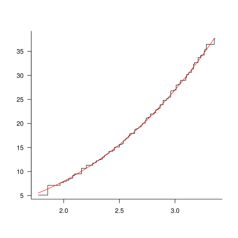
(a) $\hat{\psi}_{n,\hat{\bm{\alpha}}_{n}}$

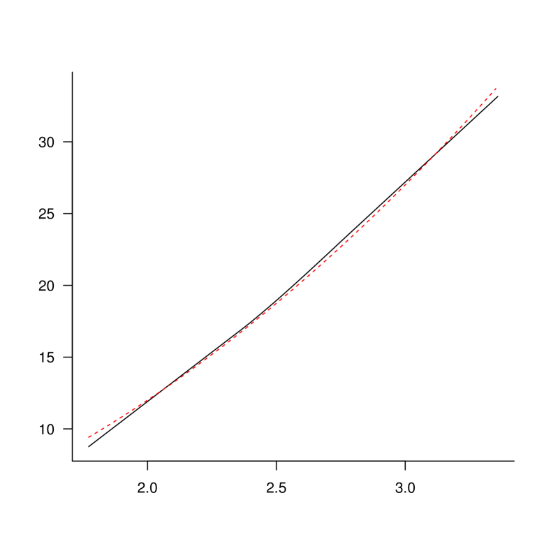
(b) $\tilde{\psi}^{\prime}_{n,\hat{\bm{\alpha}}_{n}}$

Figure 1: The estimates $\hat{\psi}_{n,\hat{\bm{\alpha}}_{n}}$ and $\tilde{\psi}^{\prime}_{n,\hat{\bm{\alpha}}_{n}}$ of $\psi_{0}$ and $\psi^{\prime}_{0}$, respectively, for $n=1000$, $d=3$ and a sample for the model used in the simulation study of Table 1. The red curves are $\psi_{0}$ and $\psi_{0}^{\prime}$. The bandwidth chosen in the estimate $\tilde{\psi}^{\prime}_{n,\hat{\bm{\alpha}}_{n}}$ was equal to the range of the values $\bm{X}^{T}\hat{\bm{\alpha}}_{n}$ times $n^{-1/7}$.

Again another formulation, directly in terms of $\bm{\alpha}$ is given in Section 4.2 below. A picture of the estimates $\hat{\psi}_{n,\hat{\bm{\alpha}}_{n}}$ and $\tilde{\psi}^{\prime}_{n,\hat{\bm{\alpha}}_{n}}$ for $n=1000$, $d=3$ and a sample for the model used in the simulation study of Table 1 below, is shown in Figure 1. For the derivative a local linear extension of the function is used at the boundary for points with a distance to the boundary smaller than the bandwidth. Note that we only need one bandwidth choice for the derivative and that this is only needed for the ESE and not for the SSE.

[Figure 1 here]

In the remainder of this section we illustrate how the score estimators can be obtained in practice using a local coordinate system representing the unit sphere. An example of such a parametrization is the spherical coordinate system ${\mathbb{S}}:[0,\pi]^{(d-2)}\times[0,2\pi]\mapsto\mathcal{S}_{d-1}:$

$$(\beta_{1},\beta_{2},\ldots,\beta_{d-1})\mapsto (\cos(\beta_{1}),\sin(\beta_{1})\cos(\beta_{2}),\sin(\beta_{1})\sin(\beta_{2})\cos(\beta_{3}),\ldots,$$

$$\sin(\beta_{1})\ldots\sin(\beta_{d-2})\cos(\beta_{d-1}),\sin(\beta_{1})\ldots\sin(\beta_{d-2})\sin(\beta_{d-1}))^{T}.$$

The map parameterizing the positive half of the sphere ${\mathbb{S}}:\{(\beta_{1},\beta_{2},\ldots,\beta_{d-1})\in[0,1]^{(d-1)}:\|\bm{\beta}\|\leq 1\}\mapsto\mathcal{S}_{d-1}:$

$$(\beta_{1},\beta_{2},\ldots,\beta_{d-1})\mapsto \left(\beta_{1},\beta_{2},\ldots,\beta_{d-1},\sqrt{1-\beta_{1}^{2}-\ldots-\beta_{d-1}^{2}}\right)^{T},$$

is another example that can be used provided $\alpha_{d}$ is positive. Prior knowledge about the position of $\bm{\alpha}_{0}$ can be derived from an initial estimate such as the LSE proposed in [1]. We illustrate the set of equations for the SSE corresponding to (5) for dimension $d=3$ and consider the parametrization

$$\mathcal{S}_{3}=\{(\alpha_{1},\alpha_{2},\alpha_{3})=(\cos(\beta_{1})\sin(\beta_{2}),\sin(\beta_{1})\sin(\beta_{2}),\cos(\beta_{2})):0\leq\beta_{1}\leq 2\pi,0\leq\beta_{2}\leq\pi\}\subset\mathbb{R}^{2}.$$ (10)

The SSE can be obtained by solving the problem

$$\left\{\begin{array}[]{l}s_{1}(\beta_{1},\beta_{2})=\frac{1}{n}\sum_{i=1}^{n}(-\sin(\beta_{1})\sin(\beta_{2})X_{i1}+\cos(\beta_{1})\sin(\beta_{2})X_{i2})\left\{Y_{i}-\hat{\psi}_{n\bm{\alpha}}(\bm{\alpha}^{T}\bm{X}_{i})\right\}=0,\\ s_{2}(\beta_{1},\beta_{2})=\frac{1}{n}\sum_{i=1}^{n}(\cos(\beta_{1})\cos(\beta_{2})X_{i1}+\sin(\beta_{1})\cos(\beta_{2})X_{i2}-\sin(\beta_{2})X_{i3})\left\{Y_{i}-\hat{\psi}_{n\bm{\alpha}}(\bm{\alpha}^{T}\bm{X}_{i})\right\}=0.\end{array}\right.$$ (13)

For the parameterizations discussed in this manuscript we have that for each map ${\mathbb{S}}$ and each parameter vector $\bm{\beta}$,

$$\left({\mathbb{S}}(\bm{\beta})\right)^{T}{\mathbb{S}}(\bm{\beta})=1.$$

Taking derivatives w.r.t. $\bm{\beta}$, we get

$$\left({\mathbb{S}}(\bm{\beta})\right)^{T}\bm{J}_{{\mathbb{S}}}(\bm{\beta})=\bm{0}^{T},$$

so that the columns of $\bm{J}_{{\mathbb{S}}}(\bm{\beta})$ belong to the space

$$\{\bm{\alpha}\}^{\perp}\equiv\left\{{\mathbb{S}}(\bm{\beta})\right\}^{\perp}\equiv\left\{\bm{z}\in\mathbb{R}^{d}:\bm{\alpha}^{T}z=0\right\}\equiv\left\{\bm{z}\in\mathbb{R}^{d}:\left({\mathbb{S}}(\bm{\beta})\right)^{T}z=0\right\}.$$

Note that for ${\mathbb{S}}(\bm{\beta})=\left(\cos(\beta_{1})\sin(\beta_{2}),\sin(\beta_{1})\sin(\beta_{2}),\cos(\beta_{2})\right)^{T}$,

$$\bm{J}_{{\mathbb{S}}}(\bm{\beta})=\begin{bmatrix}-\sin(\beta_{1})\sin(\beta_{2})&\cos(\beta_{1})\cos(\beta_{2})\\[3.00003pt] \cos(\beta_{1})\sin(\beta_{2})&\sin(\beta_{1})\cos(\beta_{2})\\[3.00003pt] 0&-\sin(\beta_{2})\end{bmatrix},$$ (14)

such that we indeed have

$${\mathbb{S}}(\bm{\beta})^{T}\bm{J}_{{\mathbb{S}}}(\bm{\beta})=\left(0,0\right),$$ (15)

for all $\bm{\beta}$. This again implies that the columns of $\bm{J}_{{\mathbb{S}}}(\bm{\beta})$ are perpendicular to the vector $\bm{\alpha}={\mathbb{S}}(\bm{\beta})$. Note moreover that the columns are linearly independent and hence form a basis for $\{\bm{\alpha}\}^{\perp}$.

It is shown in Lemma 1 of [22] that it is possible to construct a set of “local parametrization matrices” $H_{\bm{\alpha}}$ for each $\bm{\alpha}\in{\cal B}(\bm{\alpha}_{0},\delta_{0})$ with $\|\bm{\alpha}\|=1$ satisfying

$$\bm{\alpha}^{T}H_{\bm{\alpha}}=\bm{0}^{T}\quad\text{ and }\quad\left(H_{\bm{\alpha}}\right)^{T}H_{\bm{\alpha}}=\bm{I}_{d-1}$$

Their matrix $\left(H_{\bm{\alpha}}\right)^{T}$ corresponds to the Moore-Penrose pseudo-inverse of the matrix $H_{\bm{\alpha}}$ and is the analogue of our matrix $\left(\bm{J}_{{\mathbb{S}}}(\bm{\beta})\right)^{T}$ in the proof of asymptotic normality of their estimator. We will however show that the orthonormality assumption is not needed in the proofs.

4.2 The score estimator with Lagrange penalty

Instead of tackling the fact that our parameter space is essentially of dimension $d-1$ by the parametrization $\bm{\alpha}={\mathbb{S}}(\bm{\beta})$ which locally maps $\mathbb{R}^{d-1}$ into the sphere $\mathcal{S}_{d-1}$, one can introduce the restriction $\|\bm{\alpha}\|=1$ via a Lagrangian term. We then consider the problem of minimizing

$$\frac{1}{n}\sum_{i=1}^{n}\left\{Y_{i}-\hat{\psi}_{n\bm{\alpha}}(\bm{\alpha}^{T}\bm{X}_{i})\right\}^{2}+\lambda\left\{\|\bm{\alpha}\|^{2}-1\right\},$$ (16)

where $\hat{\psi}_{n\bm{\alpha}}$ is the LSE defined in Section 3 and $\lambda$ is a Lagrange parameter which we add to the sum of squared errors to deal with the identifiability of the single-index model.

Analogously to the treatment given in Section 4.1 for the SSE, we consider the derivative of (16) w.r.t. $\bm{\alpha}$, where we ignore the non-differentiability of the LSE $\hat{\psi}_{n\bm{\alpha}}$. This leads to the equation,

$$-\frac{1}{n}\sum_{i=1}^{n}\bm{X}_{i}\left\{Y_{i}-\hat{\psi}_{n\bm{\alpha}}(\bm{\alpha}^{T}\bm{X}_{i})\right\}+\lambda\bm{\alpha}=0.$$ (17)

Here $\lambda$ has to satisfy

$$\lambda=\lambda\bm{\alpha}^{T}\bm{\alpha}=\frac{1}{n}\sum_{i=1}^{n}\bm{\alpha}^{T}\bm{X}_{i}\left\{Y_{i}-\hat{\psi}_{n\bm{\alpha}}(\bm{\alpha}^{T}\bm{X}_{i})\right\}.$$ (18)

Plugging in the above expression for $\lambda$ in (17), we consider the simple score equation

$$\bm{0} =\frac{1}{n}\sum_{i=1}^{n}\bm{X}_{i}\left\{Y_{i}-\hat{\psi}_{n\bm{\alpha}}(\bm{\alpha}^{T}\bm{X}_{i})\right\}-\bm{\alpha}^{T}\left(\frac{1}{n}\sum_{i=1}^{n}\bm{X}_{i}\left\{Y_{i}-\hat{\psi}_{n\bm{\alpha}}(\bm{\alpha}^{T}\bm{X}_{i})\right\}\right)\bm{\alpha}$$

$$=\frac{1}{n}\left(\bm{I}-{\bm{\alpha}}\bm{\alpha}^{T}\right)\sum_{i=1}^{n}\bm{X}_{i}\left\{Y_{i}-\hat{\psi}_{n\bm{\alpha}}(\bm{\alpha}^{T}\bm{X}_{i})\right\},$$ (19)

where $\bm{I}$ is the $d\times d$ identity matrix. The same procedure can be derived for the ESE defined in (8) and we define the simple and efficient score estimators of the regression parameter $\bm{\alpha}_{0}$ in model (2), referred to as the score estimators using a Lagrange penalty, by zero crossing of the corresponding score functions

$$\bm{\alpha}\mapsto\frac{1}{n}\left(\bm{I}-{\bm{\alpha}}\bm{\alpha}^{T}\right)\sum_{i=1}^{n}\bm{X}_{i}\left\{Y_{i}-\hat{\psi}_{n\bm{\alpha}}(\bm{\alpha}^{T}\bm{X}_{i})\right\},$$ (20)

and

$$\bm{\alpha}\mapsto\frac{1}{n}\left(\bm{I}-{\bm{\alpha}}\bm{\alpha}^{T}\right)\sum_{i=1}^{n}\bm{X}_{i}\tilde{\psi}_{nh,\bm{\alpha}}^{\prime}\bigl{(}\bm{\alpha}^{T}\bm{X}_{i}\bigr{)}\left\{Y_{i}-\hat{\psi}_{n\bm{\alpha}}(\bm{\alpha}^{T}\bm{X}_{i})\right\},$$ (21)

respectively.

The Lagrange approach has the advantage that we do not have to deal with the reparametrization $\bm{\alpha}={\mathbb{S}}(\bm{\beta})$, but has the disadvantage that we cannot assume that $\hat{\bm{\alpha}}_{n}$ has exactly norm $1$ because we again have to deal with crossings of zero instead of exact equality to zero. One way to circumvent this problem is to normalize the solution of the right-hand side of (20) or (21) at the end of the iterations. This technique gave approximately the same solutions as the approach via reparametrization.

In Section 6 we will only derive the limiting behavior of the score estimators using the parametrization of the unit sphere, but we conjecture that both estimators, using the parametrization or the Lagrange penalty, have the same asymptotic properties. A conjecture that is further motivated by a simulation study presented in Section 7. Since the Lagrange approach avoids the mapping into the parameter space (which depends on the dimension $d$), this technique can easily be adapted for different dimensions and is favored over the parametrization score approach from a practical point of view, especially if the dimension is large. Examples of R scripts, using Rcpp, of simulation runs with this method are given in [11].

5 Linear estimates if the covariates have an elliptically symmetric distribution

It is well-known that if $\bm{X}$ has an elliptically symmetric distribution there exist link-free ordinary linear regression estimates of $\bm{\alpha}_{0}$ which are $\sqrt{n}$-convergent and have an asymptotic normal distribution, see [9]. The following estimator of this type is defined in [1] for the monotone single index model. Let $\hat{\bm{\alpha}}_{n}$ be defined by

$$\hat{\bm{\alpha}}_{n}=\mbox{argmin}_{\bm{\alpha}\in\mathbb{R}^{d}}\sum_{i=1}^{n}\left\{Y_{i}-\bm{\alpha}^{T}(\bm{X}_{i}-\bar{\bm{X}}_{n})\right\}^{2},$$ (22)

with $\bar{\bm{X}}_{n}=1/n\sum_{i=1}^{n}\bm{X}_{i}$ being the sample mean of the covariate vector. The estimate of the regression parameter $\bm{\alpha}_{0}$ in model (2) is now given by $\tilde{\bm{\alpha}}_{n}=\hat{\bm{\alpha}}_{n}/\|\hat{\bm{\alpha}}_{n}\|$. Note that $\hat{\bm{\alpha}}_{n}$ in (22) is the estimator one would use if the link function is known to be linear and one would not make the restriction that the estimator has norm 1. The following result is proved in [1].

Theorem 5.1.

Let $(\bm{X}_{1},Y_{1}),\dots,(\bm{X}_{n},Y_{n})$ be an i.i.d. sample from $(\bm{X},Y)$ such that $E(Y|\bm{X})=\psi_{0}(\bm{\alpha}_{0}\bm{X})$ almost surely, where $\psi_{0}$ is non-decreasing and $\bm{\alpha}_{0}^{T}\bm{\alpha}_{0}=1$. Suppose that $\bm{X}$ has an elliptically symmetric distribution with finite mean $\bm{\mu}\in\mathbb{R}^{d}$ and a positive definite covariance matrix $\bm{\Sigma}$. Assume, moreover, that ${\mathbb{E}}\|Y\bm{X}\|<\infty$ and that there exists a nonempty interval $[a,b]$ on which $\psi_{0}$ is strictly increasing. Then, as $n\to\infty$, the estimator $\tilde{\bm{\alpha}}_{n}=\hat{\bm{\alpha}}_{n}/\|\hat{\bm{\alpha}}_{n}\|$, where $\hat{\bm{\alpha}}_{n}$ is defined by (22), converges in probability to $\bm{\alpha}_{0}$. If, moreover, ${\mathbb{E}}Y^{2}\|\bm{X}\|^{2}<\infty$, $\sqrt{n}\{\tilde{\bm{\alpha}}_{n}-\bm{\alpha}_{0}\}$ converges in distribution to a normal distribution with mean $\bm{0}$ and covariance matrix

$$\frac{1}{c^{2}}\left(\bm{I}-\bm{\alpha}_{0}\bm{\alpha}_{0}^{T}\right)\bm{\Sigma}^{-1}\bm{\Gamma}\bm{\Sigma}^{-1}\left(\bm{I}-\bm{\alpha}_{0}\bm{\alpha}_{0}^{T}\right),\qquad c=\text{\rm Cov}\left(\psi_{0}(\bm{\alpha}_{0}^{T}\bm{X}),\bm{\alpha}_{0}^{T}\bm{X}\right)/\bm{\alpha}_{0}^{T}\bm{\Sigma}\bm{\alpha}_{0},$$

where $\bm{\Gamma}$ is the covariance matrix of $\left\{Y-{\mathbb{E}}Y-(\bm{X}-\bm{\mu})^{T}\bm{\Sigma}^{-1}\text{\rm cov}(\bm{X},Y)\right\}(\bm{X}-\bm{\mu})$.

Remark 5.2.

To avoid unnecessarily heavy notation, we denote in this section and the corresponding Appendix LABEL:supA:LFLSE the covariance matrix of $\bm{X}$ by $\bm{\Sigma}$ and the corresponding sample covariance matrix by $\bm{S}_{n}$, but note that $\bm{\Sigma}$ and $\bm{S}_{n}$ have a different meaning in the rest of the paper (see, e.g., (32) and (38)).

Instead of first calculating the estimate $\hat{\bm{\alpha}}_{n}$ in (22) and then dividing by the norm of this estimate to get norm 1, one can also consider the estimate $\hat{\bm{\alpha}}_{n,\bm{S}_{n}norm1}$, defined by

$$\hat{\bm{\alpha}}_{n,\bm{S}_{n}norm1}=\mbox{argmin}_{\bm{\alpha}\in\mathbb{R}^{d},\,\bm{\alpha}^{T}\bm{S}_{n}\bm{\alpha}=1}\sum_{i=1}^{n}\left\{Y_{i}-\bm{\alpha}^{T}(\bm{X}_{i}-\bar{\bm{X}}_{n})\right\}^{2},$$ (23)

which is more in line with the estimators of our paper, where we compute the estimators under the condition that the norm is equal to 1. Here $\bm{S}_{n}$, defined by

$$\bm{S}_{n}=\frac{1}{n}\sum_{i=1}^{n}\left\{\bm{X}_{i}-\bar{\bm{X}}_{n}\right\}\left\{\bm{X}_{i}-\bar{\bm{X}}_{n}\right\}^{T},$$

estimates the covariance $\bm{\Sigma}$, and the ordinary inner product of $\bm{x}$ and $\bm{y}$ is replaced by $\bm{x}^{T}\bm{S}_{n}\bm{y}$. Instead of the restriction $\bm{\alpha}_{0}^{T}\bm{\alpha}_{0}=1$, we now use the restriction $\bm{\alpha}_{0}^{T}\bm{\Sigma}\bm{\alpha}_{0}=1$ in the underlying model, which is estimated by the restriction $\bm{\alpha}^{T}\bm{S}_{n}\bm{\alpha}=1$ in the sample.

We will call this estimator the link-free least squares estimator (LFLSE). Since the estimator discussed above first solves another minimization problem (without a restriction on the norm), and then makes the (ordinary) norm equal to 1 by dividing by the norm, we call this the hybrid link-free least squares estimator (H-LFLSE). The two estimators are not the same, even if $\bm{\Sigma}$ is a multiple of the identity and if we use the ordinary norm for the second estimator.

Suppose now that the true index $\bm{\alpha}_{0}$ satisfies $\bm{\alpha}^{T}_{0}\bm{\Sigma}\bm{\alpha}_{0}=1$. Note that such normalization of the true parameter $\bm{\alpha}_{0}$ is always possible since it does not alter the direction of monotonicity of the link function nor the identifiability of the model. Then, following the Lagrange approach of Section 4.2, we can define the estimator $\hat{\bm{\alpha}}_{n,\bm{S}_{n}norm1}$ as the minimizer of

$$\frac{1}{n}\sum_{i=1}^{n}\left\{Y_{i}-\bm{\alpha}^{T}(\bm{X}_{i}-\bar{\bm{X}}_{n})\right\}^{2}+\lambda\{\bm{\alpha}^{T}\bm{S}_{n}\bm{\alpha}-1\},$$

for $\bm{\alpha}\in\mathbb{R}^{d}$ and for suitably chosen $\lambda\geq 0$. This time, the optimization criterion does not depend on the LSE $\hat{\psi}_{n\bm{\alpha}}$ of the link function $\psi_{0}$ and we do no longer have the crossing of zero difficulty. Note that in this case (17) is replaced by

$$-\frac{1}{n}\sum_{i=1}^{n}\bm{X}_{i}\left\{Y_{i}-\bm{\alpha}^{T}\left(\bm{X}_{i}-\bar{\bm{X}}_{n}\right)\right\}+\lambda\bm{S}_{n}\bm{\alpha}=\bm{0}.$$ (24)

Here $\lambda$ has to satisfy

$$\lambda=\lambda\bm{\alpha}^{T}\bm{S}_{n}\bm{\alpha}=\frac{1}{n}\sum_{i=1}^{n}\bm{\alpha}^{T}\left(\bm{X}_{i}-\bar{\bm{X}}_{n}\right)\left\{Y_{i}-\bm{\alpha}^{T}\left(\bm{X}_{i}-\bar{\bm{X}}_{n}\right)\right\}.$$ (25)

Since therefore

$$\lambda\bm{S}_{n}\bm{\alpha} =\frac{1}{n}\sum_{i=1}^{n}\bm{\alpha}^{T}\left(\bm{X}_{i}-\bar{\bm{X}}_{n}\right)\left\{Y_{i}-\bm{\alpha}^{T}\left(\bm{X}_{i}-\bar{\bm{X}}_{n}\right)\right\}\bm{S}_{n}\bm{\alpha}$$

$$=\frac{1}{n}\bm{S}_{n}\bm{\alpha}\bm{\alpha}^{T}\sum_{i=1}^{n}\bm{\alpha}^{T}\left(\bm{X}_{i}-\bar{\bm{X}}_{n}\right)\left\{Y_{i}-\bm{\alpha}^{T}\left(\bm{X}_{i}-\bar{\bm{X}}_{n}\right)\right\},$$

we get the equation

$$\frac{1}{n}\left(\bm{I}-\bm{S}_{n}\bm{\alpha}\bm{\alpha}^{T}\right)\sum_{i=1}^{n}\left(\bm{X}_{i}-\bar{\bm{X}}_{n}\right)\left\{Y_{i}-\bm{\alpha}^{T}\left(\bm{X}_{i}-\bar{\bm{X}}_{n}\right)\right\}=\bm{0},$$ (26)

where, if more solutions are found, the one giving the smallest criterion is chosen. For this estimator we have the following result.

Theorem 5.3.

Let $(\bm{X}_{1},Y_{1}),\dots,(\bm{X}_{n},Y_{n})$ be an i.i.d. sample from $(\bm{X},Y)$ such that $E(Y|\bm{X})=\psi_{0}(\bm{\alpha}_{0}\bm{X})$ almost surely, where $\psi_{0}$ is non-decreasing. Suppose that $\bm{X}$ has an elliptically symmetric distribution with finite mean $\mu\in\mathbb{R}^{d}$ and a positive definite covariance matrix $\bm{\Sigma}$ satisfying $\bm{\alpha}_{0}^{T}\bm{\Sigma}\bm{\alpha}_{0}=1$. Assume, moreover, that ${\mathbb{E}}|Y|<\infty$ and ${\mathbb{E}}\|\bm{X}\|^{2}<\infty$ and that there exists a nonempty interval $[a,b]$ on which $\psi_{0}$ is strictly increasing. Then, as $n\to\infty$, the estimator $\hat{\bm{\alpha}}_{n,\bm{S}_{n}norm1}$, defined by (23), converges in probability to $\bm{\alpha}_{0}$. If, moreover, ${\mathbb{E}}Y^{2}<\infty$ and ${\mathbb{E}}\|\bm{X}\|^{4}<\infty$, then $\sqrt{n}\{\hat{\bm{\alpha}}_{n,\bm{S}_{n}norm1}-\bm{\alpha}_{0}\}$ converges in distribution to a normal distribution with mean $\bm{0}$ and covariance matrix which can be computed from relation (LABEL:asymptotic_relation_elliptic_sym) given in Appendix LABEL:supA:LFLSE in the Supplementary Material.

The proof of Theorem 5.3 is given in the Supplementary Material. As an example of how one can compute the asymptotic covariance matrix, we also compute in the Supplementary Material, the asymptotic covariance matrix for the simulation setting corresponding to Table 2, given in Section 7.1. The solution of equation (26) was done by a C++ program, using Broyden’s algorithm. It is very fast and produces a norm $\{\hat{\bm{\alpha}}_{n,\bm{S}_{n}norm1}^{T}\bm{S}_{n}\hat{\bm{\alpha}}_{n,\bm{S}_{n}norm1}\}^{1/2}$ of the solution which is equal to 1 in 10 decimals, without any need of renormalization, but just by solving in $\mathbb{R}^{d}$. This illustrates the soundness of the Lagrange inspired method of estimating the parameter $\bm{\alpha}_{0}$ by solving (26) in $\mathbb{R}^{d}$ as an alternative to shifting to a lower dimensional parametrization. Since equation (4.2) for the score estimates of Section 4.2 is discontinuous and cannot be solved exactly, we use a derivative free optimization algorithm proposed by [17] instead of Broyden’s algorithm to obtain the score estimates as zero crossings of equation (4.2). More information on the computation of the score estimates in Section 4 is given in Section 7. R scripts for simulations with the estimator of Theorem 5.3, using the derivative free optimization algorithm, are also made available in [11].

Remark 5.4.

For the situation where the covariance matrix of $\bm{X}$ is assumed to be a multiple of the identity (so $\bm{X}$ has a spherically symmetric distribution), we also have a consistent estimate of $\bm{\alpha}_{0}$ if we define $\hat{\bm{\alpha}}_{n,norm1}$ by

$$\hat{\bm{\alpha}}_{n,norm1}=\mbox{argmin}_{\bm{\alpha}\in\mathbb{R}^{d},\,\bm{\alpha}^{T}\bm{\alpha}=1}\sum_{i=1}^{n}\left\{Y_{i}-\bm{\alpha}^{T}(\bm{X}_{i}-\bar{\bm{X}}_{n})\right\}^{2},$$ (27)

under the condition that $\bm{\alpha}_{0}^{T}\bm{\alpha}_{0}=1$. In this case the limiting distribution of $\sqrt{n}\{\hat{\bm{\alpha}}_{n,norm1}-\bm{\alpha}_{0}\}$ is degenerate, as is the case for the score estimators of Section 4 (see Theorems 6.5-6.7 and Remark 6.6 in Section 6). The derivation of the consistency and normal limit distribution proceeds along the same lines as the proof of Theorem 5.3, but is somewhat easier since we do not have to deal with the behavior of $\bm{S}_{n}$. However, this estimate will be inconsistent for the situation that $\bm{\Sigma}$ is not a multiple of the identity. We give the asymptotic covariance matrix in Appendix LABEL:supA:LFLSE for the simulation setting of Table 2. Remarkably, the asymptotic variances are bigger than for the estimate $\hat{\bm{\alpha}}_{n,\bm{S}_{n}norm1}$ of Theorem 5.3 in this situation.

6 Asymptotic behavior of the score estimators

In this section we first give results on the behavior of the LSE $\hat{\psi}_{n\bm{\alpha}}$ of the monotone link function and next derive the limiting distribution of the SSE and the ESE introduced in Section 4.1. The results stated in this Section are all proved in the Supplementary Material of this article.

Proposition 6.1.

Let the function $\psi_{\bm{\alpha}}$ be defined by

$$\psi_{\bm{\alpha}}(u):={\mathbb{E}}\big{[}\psi_{0}(\bm{\alpha}_{0}^{T}\bm{X})|\bm{\alpha}^{T}\bm{X}=u\big{]}.$$ (28)

Suppose that

A1. The space $\mathcal{X}$ is convex, with a nonempty interior. There exists also $R>0$ such that $\mathcal{X}\subset\mathcal{B}(0,R)$.

A2. There exists $K_{0}>0$ such that the true link function $\psi_{0}$ satisfies $|\psi_{0}(u)|\leq K_{0}$ for all $u$ in $\{\bm{\alpha}^{T}\bm{x},\bm{x}\in\mathcal{X},\bm{\alpha}\in\mathcal{S}_{d-1}\}$.

A3. There exists $\delta_{0}>0$ such that the function $\psi_{\bm{\alpha}}$ defined in (28) is monotone increasing on $\mathcal{I}_{\bm{\alpha}}:=\{\bm{\alpha}^{T}\bm{x},\bm{x}\in\mathcal{X}\}$ for all $\bm{\alpha}\in{\cal B}(\bm{\alpha}_{0},\delta_{0}):=\{\bm{\alpha}:\|\bm{\alpha}-\bm{\alpha}_{0}\|\leq\delta_{0}\}$.

Then, the functional $L_{\bm{\alpha}}$ given by,

$$\psi\mapsto L_{\bm{\alpha}}(\psi):=\int_{\mathcal{X}}\Big{(}\psi_{0}(\bm{\alpha}_{0}^{T}\bm{x})-\psi(\bm{\alpha}^{T}\bm{x})\Big{)}^{2}dG(\bm{x}),$$ (29)

admits a minimizer ${\psi}^{\bm{\alpha}}$, over the set of monotone increasing functions defined on $\mathbb{R}$, denoted by ${\cal M}$, such that $\psi^{\bm{\alpha}}$ is uniquely given by the function ($\psi_{\bm{\alpha}}$) in (28) on $\mathcal{I}_{\bm{\alpha}}=\Big{\{}\bm{\alpha}^{T}\bm{x}:\bm{x}\in\mathcal{X}\Big{\}}$.

Proposition 6.2.

Under Assumptions A1-A3 and Assumptions

A4. Let $a_{0}$ and $b_{0}$ denote the infimum and supremum of the interval $\mathcal{I}_{\bm{\alpha}_{0}}=\big{\{}\bm{\alpha}_{0}^{T}\bm{x},\ \bm{x}\in\mathcal{X}\big{\}}$. Then, the true link function $\psi_{0}$ is continuously differentiable on $(a_{0}-\delta_{0}R,b_{0}+\delta_{0}R)$, where $R$ is the same radius of assumption A1 above.

A5. The distribution of $\bm{X}$ admits a density $g$, which is differentiable on $\mathcal{X}$. Also, there exist positive constants $\underline{c}_{0}$, $\bar{c}_{0}$, $\underline{c}_{1}$ and $\bar{c}_{1}$ such that $\underline{c}_{0}\leq g\leq\bar{c}_{0}$ and $\underline{c}_{1}\leq\partial g/\partial x_{i}\leq\bar{c}_{1}$ on $\mathcal{X}$ for all $i=1,\ldots,d$.

A6. There exist $c_{0}>0$ and $M_{0}>0$ such that ${\mathbb{E}}\Big{[}|Y|^{m}\ |\bm{X}=\bm{x}\Big{]}\leq m!M_{0}^{m-2}c_{0}$ for all integers $m\geq 2$ and $\bm{x}\in\mathcal{X}$ $G$-almost surely.

we have,

$$\sup_{\bm{\alpha}\in{\cal B}(\bm{\alpha}_{0},\delta_{0})}\int\left\{\hat{\psi}_{n\bm{\alpha}}(\bm{\alpha}^{T}\bm{x})-\psi_{\bm{\alpha}}(\bm{\alpha}^{T}\bm{x})\right\}^{2}\,dG(\bm{x})=O_{p}\left((\log n)^{2}n^{-2/3}\right).$$

Discussion of the Assumptions A1-A6

Before presenting our main theorem, we would like to first comment on the different assumptions made so far. Convexity in Assumption A1 is satisfied by a wide range of distributions, and hence is not very restrictive. It implies that the support of the linear predictor $\bm{\alpha}^{T}\bm{X}$ is an interval for all $\bm{\alpha}\in{\cal B}(\bm{\alpha}_{0},\delta_{0})$, which makes things easier to visualize. This can be however generalized by assuming that $\mathcal{X}$ is the union of convex sets; a very related assumption was made in [15]. Boundedness in Assumption A1 can be relaxed and replaced by sub-Gaussianity of the distribution of $\bm{X}$; see Remark 6.3.

In Assumption A2 we only impose boundedness on the true regression function on $\{\bm{\alpha}_{0}^{T}\bm{x},\bm{x}\in\mathcal{X}\}$, whereas other estimation procedures require boundedness on the second derivative of $\psi_{0}$, as done for example in [15] and [18].

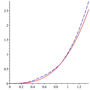
Figure 2: The real $\psi_{0}$ (red, solid) and the function $\psi_{\bm{\alpha}}$ (blue, dashed) for $\psi_{0}(x)=x^{3}$, $\alpha_{01}=\alpha_{02}=1/\sqrt{2}$ and $\alpha_{1}=1/2,\alpha_{2}=\sqrt{3}/2$, with $X_{1},X_{2}\stackrel{{\scriptstyle i.i.d}}{{\sim}}U[0,1]$.

Assumption A3 is made to enable deriving the explicit limit of the LSE $\hat{\psi}_{n\bm{\alpha}}$ for all $\bm{\alpha}\in{\cal B}(\bm{\alpha}_{0},\delta_{0})$. In the Supplementary Material it is shown that Assumption A3 is plausible by proving that for $\bm{\alpha}$ in a neighborhood of $\bm{\alpha}_{0}$ the derivative of the function $\psi_{\bm{\alpha}}$ is indeed strictly positive provided the derivative of the true link function $\psi_{0}$ stays away from zero; i.e., there exists $C>0$ such that $\psi^{\prime}_{0}\geq C$ on $\{\bm{\alpha}_{0}^{T}\bm{x},\bm{x}\in\mathcal{X}\}$. However, it can be shown that the latter condition can be made without loss of generality. A proof can be found in the Supplementary Material. The idea is to artificially add to both sides of the regression model a function of $\bm{\alpha}_{0}^{T}\bm{X}$ with a strictly positive derivative without violating the remaining assumptions. Based on several numerical experiments it seems that Assumption $A3$ remains plausible in practice even if $\bm{\alpha}$ is not not necessarily in the neighborhood of $\bm{\alpha}_{0}$. In Figure 2 we compare the true link function $\psi_{0}$ with the function $\psi_{\bm{\alpha}}$ for the model $E(Y|\bm{X})=\psi_{0}(\alpha_{01}X_{1}+\alpha_{02}X_{1})$, where $X_{1},X_{2}\stackrel{{\scriptstyle i.i.d}}{{\sim}}U[0,1]$, $\psi_{0}(\bm{x})=x^{3}$ and $\alpha_{01}=\alpha_{02}=1/\sqrt{2}$ for $\alpha_{1}=1/2,\alpha_{2}=\sqrt{3}/2$. Figure 2 shows how the function $\psi_{\bm{\alpha}}$ defined in (28) inherits the monotonicity of the true link function $\psi_{0}$.

[Figure 2 here]

The Assumptions A4 and A5, and sometimes stronger versions therereof, are made in many references on single index models. Here, they are mainly needed to be able to control the conditional expectation of $\bm{X}$ or $\bm{\alpha}^{T}_{0}\bm{X}$ given $\bm{\alpha}^{T}\bm{X}$ when $\bm{\alpha}$ is in a small neighborhood of $\bm{\alpha}_{0}$. Finally, Assumption A6 is needed to show that $\max_{1\leq i\leq n}|Y_{i}|=O_{p}(\log n)$. As noted in [1], such an assumption is satisfied in the special case where the conditional distribution of $Y|\bm{X}=\bm{x}$ belongs to an exponential family.

Remark 6.3.

Boundedness in A1 can be relaxed if we assume that $\bm{X}$ has a sub-Gaussian distribution. We recall that $\bm{X}$ is sub-Gaussian if there exists $\sigma>0$ such that for all $\bm{u}\in\mathcal{S}_{d-1}$ and $t\in\RR$

$$P(\bm{u}^{T}(\bm{X}-E(\bm{X}))>t)\leq\exp(-t^{2}/(2\sigma^{2}))\ \ \ \textrm{and}\ \ P(\bm{u}^{T}(\bm{X}-E(\bm{X}))<-t)\leq\exp(-t^{2}/(2\sigma^{2})).$$

Following similar arguments as in [1] in the proof of Proposition 6.2 given in the Supplementary Material, we can easily show that sub-Gaussianity of $\bm{X}$ implies that

$$\sup_{\bm{\alpha}\in{\cal B}(\bm{\alpha}_{0},\delta_{0})}\int\left\{\hat{\psi}_{n\bm{\alpha}}(\bm{\alpha}^{T}\bm{x})-\psi_{\bm{\alpha}}(\bm{\alpha}^{T}\bm{x})\right\}^{2}\,dG(\bm{x})=O_{p}\left((\log n)^{5/2}n^{-2/3}\right).$$

The larger power in the logarithmic factor, in comparison with the power $2$ obtained in Proposition 6.2, does not affect the conclusion about the asymptotic behavior of the score estimator since the proof still works for any uniform convergence rate of the form $(\log n)^{\gamma}n^{-2/3}$.

An important special case of sub-Gaussian distributions is that of normal distributions. Since these are also elliptically symmetric (spherically symmetric if they are centered with a diagonal covariance matrix) then it is known that an ordinary least squares estimator can consistently estimate the true direction of $\bm{\alpha}_{0}$, provided that $cov(\psi_{0}(\bm{\alpha}_{0}\bm{X}),\bm{\alpha}^{T}_{0}X)\neq 0$. The latter condition can be easily shown to hold true when $\psi_{0}$ is monotone and non-flat. This result, which goes back to [3], can be extended to any elliptically symmetric distribution, a fact that has been exploited by [9] in inverse regression. In Section 5, we discussed this simple estimator after normalization in [1] and introduced a new estimator for $\bm{\alpha}_{0}$. Both estimators are asymptotically normal.

Remark 6.4.

We would like to note that in our formulation of the model, we do assume that the predictor $\bm{X}$ and error $\varepsilon$ are independent; the assumption has also been made in e.g. [9], [4], [18], where the $\varepsilon$ is moreover assumed to be normally distributed with mean $0$ and some finite variance (not depending on $\bm{X}$). Such an assumption is unfortunately violated by many statistical models. For illustration, take the logistic regression with a Bernoulli response $Y$ and success probability $\pi(\bm{X})=\exp(\bm{\alpha}_{0}^{T}\bm{X})/(1+\exp(\bm{\alpha}_{0}^{T}\bm{X}))$. Then, the conditional variance $\text{Var}(Y|\bm{X})=\pi(\bm{X})(1-\pi(\bm{X}))=\exp(\bm{\alpha_{0}}^{T}\bm{X})/(1+\exp(\bm{\alpha_{0}}^{T}X))^{2}$, which depends on $\bm{X}$.

Proposition 6.2 is used to derive the following result on the asymptotic distribution of the SSE defined in (6) in Section 4.1.

Theorem 6.5.

Let Assumptions A1-A6 be satisfied and assume that

A7. For all $\bm{\beta}\neq\bm{\beta}_{0}$ such that ${\mathbb{S}}\left(\bm{\beta}\right)\in{\cal B}(\bm{\alpha}_{0},\delta_{0})$, the random variable

$$\text{\rm Cov}\Big{[}(\bm{\beta}_{0}-\bm{\beta})^{T}\bm{J}_{{\mathbb{S}}}(\bm{\beta})^{T}\bm{X},\psi_{0}\big{(}{\mathbb{S}}(\bm{\beta}_{0})\big{)}|\ {\mathbb{S}}(\bm{\beta})^{T}\bm{X}\Big{]},$$

is not equal to $0$ almost surely.

A8. The functions $\bm{J}_{{\mathbb{S}}}^{ij}(\bm{\beta})$, where $\bm{J}_{{\mathbb{S}}}^{ij}(\bm{\beta})$ denotes the $i\times j$ entry of $\bm{J}_{{\mathbb{S}}}(\bm{\beta})$ for $i=1,\ldots,d$ and $j=1,\ldots,d-1$ are $d-1$ times continuously differentiable on $\mathcal{C}:=\{\bm{\beta}\in\mathbb{R}^{d-1}:{\mathbb{S}}\left(\bm{\beta}\right)\in{\cal B}(\bm{\alpha}_{0},\delta_{0})\}$ and there exists $M>0$ satisfying

$$\max_{k.\leq d-1}\sup_{\bm{\beta}\in\mathcal{C}}|D^{k}\bm{J}_{{\mathbb{S}}}^{ij}(\bm{\beta})|\leq M$$ (30)

where $k=(k_{1},\ldots,k_{d})$ with $k_{j}$ an integer $\in\{0,\ldots,d-1\}$, $k.=\sum_{i=1}^{d-1}k_{i}$ and

$$D^{k}s(\bm{\beta})\equiv\frac{\partial^{k.}s(\bm{\beta})}{\partial\beta_{k_{1}}\ldots\partial\beta_{k_{d}}}.$$

We also assume that $\mathcal{C}$ is a convex and bounded set in $\mathbb{R}^{d-1}$ with a nonempty interior.

A9. $\left(\bm{J}_{{\mathbb{S}}}(\bm{\beta}_{0})\right)^{T}{\mathbb{E}}\Bigl{[}\psi_{0}^{\prime}(\bm{\alpha}_{0}^{T}\bm{X})\,\text{ Cov}(\bm{X}|\bm{\alpha}_{0}^{T}\bm{X})\Bigr{]}\left(\bm{J}_{{\mathbb{S}}}(\bm{\beta}_{0})\right)$ is nonsingular.

Let $\hat{\bm{\alpha}}_{n}$ be defined by (6). Then:

1. [Existence of a root] A crossing of zero $\hat{\bm{\beta}}_{n}$ of $\phi_{n}(\bm{\beta})$ exists with probability tending to one.

2. [Consistency]

   $$\hat{\bm{\alpha}}_{n}\stackrel{{\scriptstyle p}}{{\rightarrow}}\bm{\alpha}_{0},\qquad n\to\infty.$$

3. [Asymptotic normality] Define the matrices,

   $$\bm{A}:={\mathbb{E}}\Bigl{[}\psi_{0}^{\prime}(\bm{\alpha}_{0}^{T}\bm{X})\,\text{\rm Cov}(\bm{X}|\bm{\alpha}_{0}^{T}\bm{X})\Bigr{]},$$ (31)

   and

   $$\bm{\Sigma}:={\mathbb{E}}\left[\left\{Y-\psi_{0}(\bm{\alpha}_{0}^{T}\bm{X})\right\}^{2}\,\left\{\bm{X}-{\mathbb{E}}(\bm{X}|\bm{\alpha}_{0}^{T}\bm{X})\right\}\left\{\bm{X}-{\mathbb{E}}(\bm{X}|\bm{\alpha}_{0}^{T}\bm{X})\right\}^{T}\right].$$ (32)

   Then

   $$\sqrt{n}(\hat{\bm{\alpha}}_{n}-\bm{\alpha}_{0})\to_{d}N_{d}\left(\bm{0},\bm{A}^{-}\bm{\Sigma}\bm{A}^{-}\right),$$

   where $\bm{A}^{-}$ is the Moore-Penrose inverse of $\bm{A}$.

It can be easily seen from expression (14) for the matrix $\bm{J}_{{\mathbb{S}}}$ that the spherical coordinate system satisfies Assumption A8. In Section 7, we calculate the matrix specified in Assumptions A9 for the simulation model considered in this section and show that this assumption is indeed satisfied in the corresponding model.

Remark 6.6.

Note that $\bm{\alpha}_{0}^{T}\bm{A}=\bm{0}$ and that the normal distribution $N_{d}\left(\bm{0},\bm{A}^{-}\bm{\Sigma}\bm{A}^{-}\right)$ is concentrated on the $(d-1)$-dimensional subspace, orthogonal to $\bm{\alpha}_{0}$ and is therefore degenerate, as is also clear from its covariance matrix $\bm{A}^{-}\bm{\Sigma}\bm{A}^{-}$, which is a matrix of rank $d-1$.

For the ESE, we designed the function $\xi_{nh}$ by representing the sum of squares

$$\frac{1}{n}\sum_{i=1}^{n}\left\{Y_{i}-\psi_{\bm{\alpha}}(\bm{\alpha}^{T}\bm{X}_{i})\right\}^{2},$$

in a local coordinate system with $d-1$ unknown parameters $\bm{\beta}=(\beta_{1},\ldots,\beta_{d-1})^{T}$ followed by differentiation of the reparametrized sum of squares w.r.t. $\bm{\beta}$ where we also consider differentiation of the function $\psi_{\bm{\alpha}}$.

Theorem 6.7.

Let Assumptions A1-A8 be satisfied. Furthermore assume that the following conditions hold:

A10. The function $\psi_{\bm{\alpha}}$ is two times continuously differentiable on ${\cal I}_{\bm{\alpha}}$ for all $\bm{\alpha}$.

A11. $\left(\bm{J}_{{\mathbb{S}}}(\bm{\beta})\right)^{T}{\mathbb{E}}\Bigl{[}\psi_{0}^{\prime}(\bm{\alpha}_{0}^{T}\bm{X})^{2}\,\text{ Cov}(\bm{X}|\bm{\alpha}_{0}^{T}\bm{X})\Bigr{]}\bm{J}_{{\mathbb{S}}}(\bm{\beta})$ is nonsingular.

Let $\tilde{\bm{\alpha}}_{n}$ be defined by (8) and suppose $h\asymp n^{-1/7}$. Then:

1. [Existence of a root] A crossing of zero $\tilde{\bm{\beta}}_{n}$ of $\xi_{nh}(\bm{\beta})$ exists with probability tending to one.

2. [Consistency]

   $$\tilde{\bm{\alpha}}_{n}\stackrel{{\scriptstyle p}}{{\rightarrow}}\bm{\alpha}_{0},\qquad n\to\infty.$$

3. [Asymptotic normality] Define the matrices,

   $$\tilde{\bm{A}}:={\mathbb{E}}\Bigl{[}\psi_{0}^{\prime}(\bm{\alpha}_{0}^{T}\bm{X})^{2}\,\text{ Cov}(\bm{X}|\bm{\alpha}_{0}^{T}\bm{X})\Bigr{]},$$ (33)

   and

   $$\tilde{\bm{\Sigma}}:={\mathbb{E}}\left[\left\{Y-\psi_{0}(\bm{\alpha}_{0}^{T}\bm{X})\right\}^{2}\psi_{0}^{\prime}(\bm{\alpha}_{0}^{T}\bm{X})^{2}\left\{\bm{X}-{\mathbb{E}}(\bm{X}|\bm{\alpha}_{0}^{T}\bm{X})\right\}\left\{\bm{X}-{\mathbb{E}}(\bm{X}|\bm{\alpha}_{0}^{T}\bm{X})\right\}^{T}\right].$$ (34)

   Then

   $$\sqrt{n}(\tilde{\bm{\alpha}}_{n}-\bm{\alpha}_{0})\to_{d}N_{d}\left(\bm{0},\tilde{\bm{A}}^{-}\tilde{\bm{\Sigma}}\tilde{\bm{A}}^{-}\right),$$

   where $\tilde{\bm{A}}^{-}$ is the Moore-Penrose inverse of $\tilde{\bm{A}}$.

Remark 6.8.

The asymptotic variance of the estimator $\tilde{\bm{\alpha}}_{n}$ is similar to that obtained for the “efficient” estimates proposed in [29] and in [21]. The efficient score function for the semi-parametric single index model is

$$\tilde{\ell}_{\bm{\alpha}_{0},\psi_{0}}(\bm{x},y)=\frac{y-\psi\left(\bm{\alpha}_{0}^{T}\bm{x}\right)}{\sigma^{2}(\bm{x})}\psi^{\prime}\left(\bm{\alpha}_{0}^{T}\bm{x}\right)\left\{\bm{x}-\frac{{\mathbb{E}}\left\{\sigma^{-2}(\bm{X})\bm{X}|\bm{\alpha}_{0}^{T}\bm{X}=\bm{\alpha}_{0}^{T}\bm{x}\right\}}{{\mathbb{E}}\left\{\sigma^{-2}(\bm{X})|\bm{\alpha}_{0}^{T}\bm{X}=\bm{\alpha}_{0}^{T}\bm{x}\right\}}\right\}.$$

More details on the efficiency calculations can be found in e.g. [27], chapter 25 for a general description of the efficient score functions and in [8] or [21] for the efficient score in the single index model.

In a homoscedastic model with var$(Y|\bm{X}=\bm{x})=\sigma^{2}$, where $\sigma^{2}$ is independent of covariates $\bm{x}$, the asymptotic variance equals $\sigma^{2}\tilde{\bm{A}}^{-}$ which is the same as the inverse of ${\mathbb{E}}(\tilde{\ell}_{\bm{\alpha}_{0},\psi_{0}}(\bm{X},Y)\tilde{\ell}_{\bm{\alpha}_{0},\psi_{0}}(\bm{X},Y)^{T})$. This indeed shows that our estimate defined in (8) is efficient in the homoscedastic model. As also explained in Remark 2 of [21], our estimator has also a high relative efficiency with respect to the optimal semi parametric efficiency bound if the constant variance assumption provides a good approximation to the truth.

6.1 The asymptotic relation for the score estimators

To obtain the asymptotic normality result of the SSE $\hat{\bm{\alpha}}_{n}$ given in Theorem 6.5, we prove in the Supplementary Material that the following asymptotic relationship holds for $\hat{\bm{\beta}}_{n}$:

$$\bm{B}\left(\hat{\bm{\beta}}_{n}-\bm{\beta}_{0}\right) =\int\left(\bm{J}_{{\mathbb{S}}}(\bm{\beta}_{0})\right)^{T}\left\{\bm{x}-{\mathbb{E}}(\bm{X}|{\mathbb{S}}(\bm{\beta}_{0})^{T}\bm{X}={\mathbb{S}}(\bm{\beta}_{0})^{T}\bm{x})\right\}\left\{y-\psi_{0}\bigl{(}{\mathbb{S}}(\bm{\beta}_{0})^{T}\bm{x}\bigr{)}\right\}\,d\bigl{(}{\mathbb{P}}_{n}-P_{0}\bigr{)}(\bm{x},y)$$

$$\qquad+o_{p}\left(n^{-1/2}\right).$$

where

$$\bm{B}=\left(\bm{J}_{{\mathbb{S}}}(\bm{\beta}_{0})\right)^{T}{\mathbb{E}}\Bigl{[}\psi_{0}^{\prime}({\mathbb{S}}(\bm{\beta}_{0})^{T}\bm{X})\,\text{ Cov}(\bm{X}|{\mathbb{S}}(\bm{\beta}_{0})^{T}\bm{X})\Bigr{]}\left(\bm{J}_{{\mathbb{S}}}(\bm{\beta}_{0})\right)=\left(\bm{J}_{{\mathbb{S}}}(\bm{\beta}_{0})\right)^{T}\bm{A}\,\bm{J}_{{\mathbb{S}}}(\bm{\beta}_{0}),$$ (35)

in $\mathbb{R}^{(d-1)\times(d-1)}$. We assume in Assumption A9 that $\bm{B}$ is invertible so that

$$\sqrt{n}\left(\hat{\bm{\beta}}_{n}-\bm{\beta}_{0}\right)$$

$$=\sqrt{n}\bm{B}^{-1}\int\left(\bm{J}_{{\mathbb{S}}}(\bm{\beta}_{0})\right)^{T}\left\{\bm{x}-{\mathbb{E}}(\bm{X}|{\mathbb{S}}(\bm{\beta}_{0})^{T}\bm{X}={\mathbb{S}}(\bm{\beta}_{0})^{T}\bm{x})\right\}\left\{y-\psi_{0}\bigl{(}{\mathbb{S}}(\bm{\beta}_{0})^{T}\bm{x}\bigr{)}\right\}\,d\bigl{(}{\mathbb{P}}_{n}-P_{0}\bigr{)}(\bm{x},y)+o_{p}(1)$$

$$\qquad\to_{d}N(\bm{0},\bm{\Pi}),$$

where

$$\bm{\Pi}=\bm{B}^{-1}\left(\bm{J}_{{\mathbb{S}}}(\bm{\beta}_{0})\right)^{T}\bm{\Sigma}\,\bm{J}_{{\mathbb{S}}}(\bm{\beta}_{0})\,\bm{B}^{-1}\in\mathbb{R}^{(d-1)\times(d-1)}.$$ (36)

The limit distribution of the single index score estimator $\hat{\bm{\alpha}}_{n}$ defined in (6) now follows by an application of the delta-method and we conclude that

$$\sqrt{n}(\hat{\bm{\alpha}}_{n}-\bm{\alpha}_{0}) =\sqrt{n}\left({\mathbb{S}}\big{(}\hat{\bm{\beta}}_{n}\big{)}-{\mathbb{S}}\left(\bm{\beta}_{0}\right)\right)=J_{{\mathbb{S}}}(\bm{\beta}_{0})\sqrt{n}(\hat{\bm{\beta}}_{n}-\bm{\beta}_{0})+o_{p}(1)$$

$$\to_{d}N_{d}\left(\bm{0},J_{{\mathbb{S}}}(\bm{\beta}_{0})\bm{\Pi}\left(J_{{\mathbb{S}}}(\bm{\beta}_{0})\right)^{T}\right)=N_{d}\left(\bm{0},{\bm{A}}^{-}{\bm{\Sigma}}{\bm{A}}^{-}\right),$$

where the last equality follows from the following lemma.

Lemma 6.9.

Let the matrix $\bm{A}$ be defined by (31) and let $\bm{A}^{-}$ be the Moore-Penrose inverse of $\bm{A}$. Then

$${\bm{A}}^{-}=\bm{J}_{{\mathbb{S}}}(\bm{\beta}_{0})\left\{\left(\bm{J}_{{\mathbb{S}}}(\bm{\beta}_{0})\right)^{T}{\bm{A}}\bm{J}_{{\mathbb{S}}}(\bm{\beta}_{0})\right\}^{-1}\left(\bm{J}_{{\mathbb{S}}}(\bm{\beta}_{0})\right)^{T}=\bm{J}_{{\mathbb{S}}}(\bm{\beta}_{0})\bm{B}^{-1}\left(\bm{J}_{{\mathbb{S}}}(\bm{\beta}_{0})\right)^{T}.$$

The proof of Lemma 6.9 is given the Supplementary Material.

The asymptotic variance of the ESE can be obtained similarly to the derivations of the asymptotic limiting distribution for the SSE. First the asymptotic variance is expressed in terms of the parametrization ${\mathbb{S}}$ as in (36) and next, similar to Lemma 6.9, equivalence to the expression $\tilde{\bm{A}}^{-}\tilde{\bm{\Sigma}}\tilde{\bm{A}}^{-}$ given in Theorem 6.7 is proved.

7 Computation and finite sample behavior of the score estimators

In this section we investigate the applicability and the performance of the score estimates of Section 4 in practice. We first describe the optimization algorithm used to obtain the score estimates and next include two simulation studies and compare the score estimates with alternative estimates for the monotone single index model. In the first simulation setting, given in Section 7.1, we illustrate that the variance of the score estimates converges to the asymptotic variances derived in Section 6. We also compare the score estimates with the maximum rank correlation estimate (MRCE) proposed by [14], and the Effective Dimension Reduction Estimate (EDRE), proposed in [18] and the Penalized Least Squares Estimate, proposed in [22]. To compute the latter two estimates, we used the R packages EDR and simest, respectively. As for the alternative $\sqrt{n}$-consistent “link-free" estimates of Section 5, the MRCE also does not depend on an estimate of the link function $\psi_{0}$. Finally, we discuss the convergence of the variances for the least squares estimate (LSE) minimizing the sum of squared errors $S_{n}$ defined in (1) w.r.t. $(\psi,\bm{\alpha})$, for which the asymptotic distribution is still an open problem.

In the second simulation setting in Section 7.2, we investigate the quality of the score estimates if the dimension of the parameter space increases and investigate the finite sample behavior of different efficient estimates in the single index model.

By the discontinuous nature of the score functions given in Section 4, we introduced the concept of a zero-crossing in Definition 4.1. It is not possible to solve the score equations exactly and we therefore search the crossing of zero, by minimizing the sum of squared component score functions over all possible values of $\bm{\beta}$ (parametrization approach of Section 4.1), respectively $\bm{\alpha}$ (Lagrange approach of Section 4.2). Note that the crossing of zero of the score function is equivalent to the minimizer of the sum of squared component scores so that the minimization procedure is justified. Due to the non-convex nature of the optimization function, standard optimization approaches based on a convex loss function cannot be used to obtain the score estimates.

We use a derivative free optimization algorithm proposed by [17] to obtain the score estimates. The method is a pattern-search optimization method that does not require the objective function to be continuous. The algorithm starts from an initial estimate of the minimum and looks for a better nearby point using a set of $2d$ equal step sizes along the coordinate axes in each direction, first making a step in the direction of the previous move. For the object function we take the sum of the squared values of the component functions, which achieves a minimum at a crossing of zero. If in no direction an improvement is found, the step size is halved, and a new search for improvement is done, with the reduced step sizes. This is repeated until the step size has reached a prespecified minimum. A very clear exposition of the method is given in [26], Section 4.3. In this paper also convergence proofs for the optimization algorithm are presented. The optimization algorithm depends on a starting value for the regression parameters. In our simulations we used the true parameter values as starting values. In practice, we propose to search over a random grid of starting values on the unit sphere and select the estimate that results the smallest prediction error $\sum_{i=1}^{n}\{Y_{i}-\hat{\psi}_{n\hat{\bm{\alpha}}_{n}}(\hat{\bm{\alpha}_{n}}^{T}\bm{X}_{i})\}^{2}$ among all different initial searches as a final starting value to obtain the score estimate.

7.1 Simulation 1: The asymptotic properties of the score estimators

In this section, we illustrate the asymptotic properties of the SSE and the ESE given in Section 6 in the model

$$Y=\psi_{0}(\bm{\alpha}_{0}^{T}\bm{X})+\varepsilon,\quad,\psi_{0}(\bm{x})=x^{3},\quad\alpha_{01}=\alpha_{02}=\alpha_{03}=1/\sqrt{3},\quad\quad X_{1},X_{2},X_{3}\stackrel{{\scriptstyle i.i.d}}{{\sim}}U[1,2],\quad\varepsilon\sim N(0,1),$$

where $\varepsilon$ is independent of the covariate vector $\bm{X}=(X_{1},X_{2},X_{3})^{T}$. For this model, we have

$$\bm{A}=\frac{17}{15}\begin{bmatrix}2&-1&-1\\[3.00003pt] -1&2&-1\\[3.00003pt] -1&-1&2\end{bmatrix}\quad\text{,}\quad\bm{\Sigma}=\frac{1}{36}\begin{bmatrix}2&-1&-1\\[3.00003pt] -1&2&-1\\[3.00003pt] -1&-1&2\end{bmatrix}\quad\text{ and}\quad\tilde{\bm{A}}=\tilde{\bm{\Sigma}}=\frac{89953}{7560}\begin{bmatrix}2&-1&-1\\[3.00003pt] -1&2&-1\\[3.00003pt] -1&-1&2\end{bmatrix},$$

where the matrices $\bm{A},\bm{\Sigma},\tilde{\bm{A}}$ and $\tilde{\bm{\Sigma}}$ are defined in (31), (32), (33) and (34) respectively. Note that the rank of the matrices is equal to $d-1=2$. For this model, using the spherical coordinate system in three dimension introduced in (10), we get for the matrix specified in Assumption A9 that

$$\left(\bm{J}_{{\mathbb{S}}}(\bm{\beta}_{0})\right)^{T}{\mathbb{E}}\Bigl{[}\psi_{0}^{\prime}(\bm{\alpha}_{0}^{T}\bm{X})\,\text{Cov}(\bm{X}|\bm{\alpha}_{0}^{T}\bm{X})\Bigr{]}\left(\bm{J}_{{\mathbb{S}}}(\bm{\beta}_{0})\right)=\begin{bmatrix}\frac{17}{15}&0\\[3.00003pt] 0&\frac{17}{10}\end{bmatrix},$$

which illustrates that the nonsingularity in Assumption A9 is indeed satisfied in this simulation setup. The same holds for the matrix given in Assumption A10.

The asymptotic variance of $\hat{\bm{\alpha}}_{n}$ resp. $\tilde{\bm{\alpha}}_{n}$ defined in Theorem 6.5 resp. Theorem 6.7 is equal to

$$\bm{A}^{-}\bm{\Sigma}\bm{A}^{-}=\frac{25}{2601}\begin{bmatrix}2&-1&-1\\[3.00003pt] -1&2&-1\\[3.00003pt] -1&-1&2\end{bmatrix}\quad\text{ resp. }\quad\tilde{\bm{A}}^{-}\tilde{\bm{\Sigma}}\tilde{\bm{A}}^{-}=\tilde{\bm{A}}^{-}=\frac{840}{89953}\begin{bmatrix}2&-1&-1\\[3.00003pt] -1&2&-1\\[3.00003pt] -1&-1&2\end{bmatrix}.$$ (37)

We compare the estimates with the least squares estimates minimizing the sum of squared errors $S_{n}$ defined in (1) w.r.t. $(\psi,\bm{\alpha})$ and with the MRCE proposed by [14]. This estimator is defined by the maximizer of

$$H_{n}(\bm{\alpha}):=\frac{1}{n(n-1)}\sum_{i\neq j}\{Y_{i}>Y_{j}\}\{\bm{\alpha}^{T}\bm{X}_{i}>\bm{\alpha}^{T}\bm{X}_{j}\},$$

over all $\bm{\alpha}\in\mathcal{S}_{d-1}$. The MRCE is proved to be a $\sqrt{n}$-consistent and asymptotically normal estimator of the regression parameter in the monotone single index model by [24], who gave an expression for the asymptotic covariance matrix in an (implicit) $(d-1)$-dimensional representation in his Theorem 4 on p. 133. If, in accordance with the parametrization methods of our paper, we turn this into an expression in terms of our $d$-dimensional representation, we obtain as the asymptotic covariance matrix of the MRCE $\bm{V}^{-}\bm{S}\bm{V}^{-}$ where

$$\bm{S}={\mathbb{E}}\left[\left\{\bm{X}-{\mathbb{E}}(\bm{X}|\bm{\alpha}_{0}^{T}\bm{X})\right\}\left\{\bm{X}-{\mathbb{E}}(\bm{X}|\bm{\alpha}_{0}^{T}\bm{X})\right\}^{T}S(Y,\bm{\alpha}_{0}^{T}\bm{X})^{2}g_{0}(\bm{\alpha}_{0}^{T}\bm{X})^{2}\right],$$ (38)

and $\bm{V}^{-}$ is the Moore-Penrose inverse of

$$\bm{V}={\mathbb{E}}\left[\left\{\bm{X}-{\mathbb{E}}(\bm{X}|\bm{\alpha}_{0}^{T}\bm{X})\right\}\left\{\bm{X}-{\mathbb{E}}(\bm{X}|\bm{\alpha}_{0}^{T}\bm{X})\right\}^{T}S_{2}(Y,\bm{\alpha}_{0}^{T}\bm{X})g_{0}(\bm{\alpha}_{0}^{T}\bm{X})^{2}\right],$$

and $g_{0}$ is the density of $\bm{\alpha}_{0}^{T}\bm{X}$ and $S$ and $S_{2}$ are defined by

$$S(y,u)=E\left[1_{\{y>Y\}}-1_{\{y<Y\}}\bigm{|}\bm{\alpha}_{0}^{T}\bm{X}=u\right],\qquad S_{2}(y,u)=\frac{\partial}{\partial u}S(y,u).$$

It is clear from our simulations that the factor $2$ in front of $\bm{V}$ in (20) of [24] cannot be correct and indeed [4] have a note on p. 361 of their paper, attributed to Myoung-Jae Lee that this factor $2$ should not be there.
To obtain the LSE and MRCE under the identifiability restriction $\|\bm{\alpha}_{0}\|=1$, we also consider the parametrization of the unit sphere and first rewrite the optimization function

$$\tilde{S}_{n}(\bm{\beta}):=\frac{1}{n}\sum_{i=1}^{n}\Big{\{}Y_{i}-\hat{\psi}_{n{\mathbb{S}}(\bm{\beta})}({\mathbb{S}}(\bm{\beta})^{T}\bm{X}_{i})\Big{\}}^{2},$$ (39)

for the LSE and

$$\tilde{H}_{n}(\bm{\beta}){:=}\frac{1}{n(n-1)}\sum_{i\neq j}\{Y_{i}>Y_{j}\}\{{\mathbb{S}}(\bm{\beta})^{T}\bm{X}_{i}>{\mathbb{S}}(\bm{\beta})^{T}\bm{X}_{j}\},$$ (40)

for the MRCE in terms of the $(d-1)=2$ dimensional vector $\bm{\beta}$ using the spherical coordinate system in three dimensions. Next we use the optimization algorithm by [17], discussed above, to minimize $\tilde{S}_{n}$ respectively maximize $\tilde{H}_{n}$ w.r.t. $\bm{\beta}$ to end up with a LSE respectively MRCE of the regression parameter that has length one and hence satisfies our identifiability restriction.

To illustrate the link-free least squares estimates H-LFLSE and LFLSE in Section 5, we also consider normally distributed covariates $\bm{X}$, $X_{i}\stackrel{{\scriptstyle i.i.d}}{{\sim}}N(0,1)$ for $i=1,\ldots,d$. Since the asymptotic results for the score estimates of section 4 are proven under the assumption of bounded covariates only, this simulation provides further insight in the convergence of the variances of our score estimates in a model where not all Assumptions given in Section 6 are satisfied. Since the LFLSE does not depend on the behavior of the LSE $\hat{\psi}_{n\bm{\alpha}}$ and no longer suffer from the crossing of zero difficulties, we used Broyden’s method for solving nonlinear equations in higher dimensions to obtain the LFLSE, which is very fast and of quasi Newton type.

For sample sizes $n=100,500,1000,2000,5000$ and $n=10000$ we generated $N=5000$ datasets and show, in Tables 1 and 2, the mean and $n$ times the covariance of the estimates. Tables 1 and 2 also show the asymptotic values to which the results for the SSE and the ESE should converge based on Theorem 6.5 and Theorem 6.7 respectively. For the limiting variance of the MRCE, we used the description above. The asymptotic distributions of the H-LFLSE and LFLSE, on the other hand, are only derived for the normally distributed and not the uniformly distributed covariate setting, since the latter setting does not satisfy the condition of elliptic symmetry. The variances to which the H-LFLSE and the LFLSE should converge are given in Section 5. The limiting distribution of the LSE is still unknown and therefore no asymptotic results are provided for the LSE in Tables 1 and 2.

[Tables 1 and 2]

For the two simulation studies, the results shown in Tables 1 and 2 show convergence of $n$ times the variance-covariance matrices towards the asymptotic values. The performance of the ESE is slightly better than the performance of the SSE; the difference between the asymptotic limiting variances is smaller in the model with uniform$[1,2]$ covariates $X_{i}$ than the difference in the model with standard normal covariates $X_{i}$. Although the model with standard normal covariates violates Assumptions A1, A2 and A4 given in Section 6, our proposed score estimates perform reasonably well. We added In Table 1 the values for the estimators EDRE (“Effective Dimension Reduction Estimate”) and PLSE (“Penalized Least Squares Estimate”) that are further studied in Subsection 7.2.

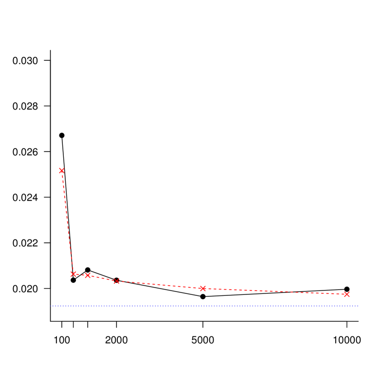
(a) SSE

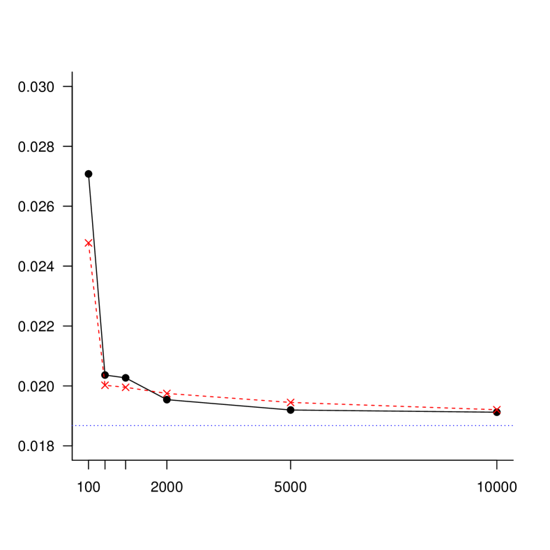
(b) ESE

Figure 3: Simulation model ($X_{i}\sim U[1,2],d=3$): $n\mapsto n\cdot$var$(\hat{\alpha}_{3n})$ for (a) the SSE and (b) the ESE using the parametrization approach (red,dashed, $\times$) Lagrange approach (black, solid, $\bullet$). The blue, dotted line indicates the asymptotic variance of the score estimates.

Figure 3 illustrates the similarity for $n\cdot$var$(\hat{\alpha}_{3n})$ between the the score estimates obtained with either the parametrization or Lagrange approach. Similar results are obtained for the other variances reported in Table 1, which supports the conjecture that the asymptotic properties of the score estimates with Lagrange penalty term (Section 4.2) are equivalent to the asymptotic results presented in Section 6 for the estimates obtained via a parametrization of the unit sphere (Section 4.1).

[Figure 3 here]

The performance of the link-free estimates MRCE, H-LFLSE and LFLSE is considerably worse than the performances of our proposed score estimates in all simulation settings. In the model with standard normal covariates, the variances of these link-free estimates are remarkably larger than the variances of the score estimates and the LSE. This might be caused by the fact that these estimates are not based on an estimate of the link function and hence do not take information about this link function into account. It is clear from our experiments that the link-free estimates are for sure not the most preferred estimates to use in the monotone single index model, even if the conditions for their use are satisfied.

Estimation of the link function $\hat{\psi}_{n\bm{\alpha}}$ is very straightforward. Since the number of jump points of the LSE $\hat{\psi}_{n\bm{\alpha}}$ is of the order $n^{1/3}$, estimation of the smooth derivate estimate $\tilde{\psi}_{nh\bm{\alpha}}^{\prime}$ only requires one additional summation over these $O(n^{1/3})$ jump points for each of the $n$ observations. The computation time for the score estimates is relatively fast (a more in depth study of the computation time is given in Section 7.2). Although the MRCE does not depend on an estimate of the link function, a double sum is needed for the calculation of the criterion function $\tilde{H}_{n}$ which increases the computation time considerably when the sample size is large. Since the H-LFLSE only depends on an ordinary least squares algorithm and since we can use Broyden’s algorithm for the LFLSE, these estimates do not require a hard optimization algorithm and the computation of the LFLSE and the H-LFLSE requires less than a second in all our simulations.

The behavior of the LSE is rather remarkable. Table 1 suggests an increase of $n$ times the covariance matrix, whereas Table 2 suggests a decrease. The results presented in Table 2 show that the performance of the LSE is better than the performance of the SSE when $X_{i}\sim N(0,1)$. For the model with uniform covariates, summarized in Table 1, our proposed score estimates are better than the LSE. The variances for the LSE presented in Tables 1 and 2 suggest that the rate of convergence for the LSE is faster than the cube-root $n$ rate proved in [1].

7.2 Simulation 2: Further comparisons and the behavior of the estimators if the covariates have a higher dimension

In this section we illustrate the applicability of the score estimates given in Section 4.2 when the dimension of the covariate space increases. We also compare our estimates with the Effective Dimension Reduction Estimate (EDRE) (see [18]) and the Smooth Penalized Least Squares estimate (PLSE) (see [21]). Here we use again the R packages EDR and simest available on CRAN, just as in the previous simulation. We use the Lagrange approach to the computation of the SSE and ESE. The computation relies on C++ programs which are used in R (via Rcpp) scripts, see [11]. The following results can be reproduced by running the R scripts, given there.

We consider the model of Table 2 more generally:

$$Y=\psi_{0}(\bm{\alpha}_{0}^{T}\bm{X})+\varepsilon,\quad,\psi_{0}(\bm{x})=x^{3},\quad\bm{\alpha}=d^{-1/2}(1,\dots,1)^{T},\quad\quad X_{i}\stackrel{{\scriptstyle i.i.d}}{{\sim}}N(0,1),\quad\varepsilon\sim N(0,1),$$

where (dimension) $d=5,10,15,25$ (the case $d=3$ was considered in Table 2). The estimation error is measured via $\sqrt{n/d}\,\|\hat{\bm{\alpha}}_{n}-\bm{\alpha}_{0}\|_{2}$, where $\|\cdot\|_{2}$ is the Euclidean norm. The results are compared with what the asymptotic distribution of the efficient estimate would give. The asymptotic distribution of efficient estimates of $\bm{\alpha}_{0}$ is, for general $d\geq 2$, given by a degenerate normal distribution with mean zero and covariance matrix

$$\bm{\Sigma}_{d}=\frac{1}{27d}\left\{d\bm{I}-\bm{1}\cdot\bm{1}^{T}\right\},$$ (41)

where $\bm{I}$ is the $d\times d$ identity matrix and $\bm{1}$ is the column vector with $d$ components, equal to $1$. The special case $d=3$ was used in Table 2. Results of these experiments are given in Figures 4 to 6. Figures 4 and 5 give the behavior of the $L_{2}$-distance for different dimensions and sample sizes $n=100$ and $n=1000$, respectively. Figure 6 gives the computing time in seconds for sample size $n=1000$. Clearly EDR needs the longest computing time.

[Figures 4 to 6 here]

All algorithms depend on starting values for the regression parameter. For the EDRE and SSE we do not have to specify tuning parameters, although for the EDRE there are if fact tuning parameters, hidden in the package EDR. Some of the algorithms have more need for a reasonable starting value than others. For example, one can start SSE and LSE at a starting value having a larger distance to the real value of $\bm{\alpha}_{0}$ than others, such as the ESE. One can solve this isssue for example by starting the ESE algorithm from the value obtained by the LSE, which is itself started from arbitrary starting values, such as $(1,0,\dots,0)$ or from a value, found by a preliminary search on starting values of the LSE algorithm, using the sum of the squared errors as criterion (see the remark on this issue just before section 7.1 above). Clearly more research for this selection procedure is necessary.

The bandwidth for the computation of the estimate of the derivative $\psi_{0}^{\prime}$ of $\psi_{0}$ in the algorithm for the ESE is set equal to $h=\tfrac{1}{2}\tilde{c}n^{-1/7}$ where $\tilde{c}$ equals the range $\bm{\alpha}^{T}\bm{X}_{1},\ldots,\bm{\alpha}^{T}\bm{X}_{n}$ and $\bm{\alpha}$ is the current estimate of $\bm{\alpha}_{0}$ during the iterations. This choice gave satisfactory results in all our experiments. We do not discuss bandwidth selection procedures in this manuscript, but note that the bootstrap techniques discussed in [12] and [13] for the current status model, can also be investigated further to select the bandwidth of the ESE in the monotone single index model in practice. For the PLSE (generalized) cross-validation can be used to select the smoothing parameter. In our experiments; we took the smoothness penalty for the PLSE equal to $0.1$ (after some preliminary experimentation). The EDR method uses an average derivative estimate (derivative w.r.t. the covariate $X$) as starting value, but computing this estimate is done within the package.

The results in Figures 4 to 6 suggest that the asymptotically efficient estimates ESE and PLSE have the best behavior. The results for the EDRE deteriorate significantly with increasing dimension, both in $L_{2}$-error and computing time. The LSE has remarkably good behavior and there is certainly the suggestion that its rate of convergence is faster than $n^{1/3}$ for the present model.

8 Summary

In this paper we introduce estimates for the regression parameter in the monotone single index model. Our estimates are obtained via the zero-crossing of an unsmooth score equation derived from the sum of squared errors and depend on the behavior of the LSE of the underlying monotone link function. We prove $\sqrt{n}$-consistency and asymptotic normality of our estimates and therefore, for the first time, define estimates that depend on the cube-root-$n$ consistent LSE of the link function which still converge at the parametric rate to the true regression parameter in the monotone single index model. By introducing a score approach similar to the M-approach for the profile LSE, where simultaneous minimization is over $\bm{\alpha}$ and the link function, we avoid the difficulties that arise when analyzing the limiting behavior of the profile LSE. This novel result in the field of shape constrained statistics will hopefully help us to further understand the behavior of the profile LSE in the monotone single index model, for which the limiting distribution is still unknown.

We consider two different score estimates, one very simple one that does not require any smoothing technique and one efficient estimate that is based on a smooth estimate of the derivative of the link function. This derivative estimate depends again only on the LSE of the link function, but, in contrast with the LSE itself, also on a kernel which is integrated w.r.t. the jumps of the LSE. We use two techniques to ensure that the norm of the regression parameter estimate is one. The first approach uses a parametrization of the unit sphere in $d-1$ dimensions. In the second method, motivated by the Lagrange approach, we directly solve an equation in dimension $d$ for the parameter $\bm{\alpha}$ and divide by the norm at the end of the iterations.

Since our score functions depend on the piecewise constant LSE of the link function, we obtain unsmooth score functions that might not have an exact root. We therefore work with zero-crossings instead of exact zeros and prove that there indeed always exists a value for the regression parameter where the score functions cross zero.

We compare our score estimates with link-free estimates of the single index parameters that avoid estimation of the link function. To that end, we also introduce a link-free least squares estimate, conditioned to have norm one and derive the asymptotic variance of this link-free estimate for the situation where we have elliptically symmetric distributions for the covariates $\bm{X}$ (like the normal $\bm{X}$ in the simulation setting of Table 2). Since this estimate no longer depends on the LSE of the link function, the crossing of zero issues disappear and we can solve the corresponding score equation exactly. This also illustrates the applicability of the method motivated by the Lagrangian formulation, which avoids the reparametrization. Our simulations clearly show that our score estimates have a better behavior than the link-free estimates, even if the conditions for application of the latter methods are fulfilled.

A numerical comparison between the score estimate and other estimates for the single index model reveals that our score estimates perform well in higher dimensions. Our computer experiments moreover point out that the Lagrange score approach can easily be used in higher dimensions.

(a) $d=5$

(b) $d=10$

(c) $d=15$

(d) $d=25$

Figure 4: Boxplots of $\sqrt{n/d}\,\|\hat{\bm{\alpha}}_{n}-\bm{\alpha}_{0}\|_{2}$ for $n=100$ and for (a) $d=5$, (b) $d=10$, (c) $d=15$ and (d) $d=25$ and 1000 replications for the EDR, SSE, ESE, LSE and PLSE. The algorithms for SSE, ESE, LSE and PLSE were started at $\bm{\alpha}_{0}$. The asymptotic distribution is generated via $1000$ draws from the degenerate limiting normal distribution for the efficient estimates, with mean zero and covariance matrix $\bm{\Sigma}_{d}$, defined by (41).

(a) $d=5$

(b) $d=10$

(c) $d=15$

(d) $d=25$

Figure 5: Boxplots of $\sqrt{n/d}\,\|\hat{\bm{\alpha}}_{n}-\bm{\alpha}_{0}\|_{2}$ for $n=1000$ and for (a) $d=5$, (b) $d=10$, (c) $d=15$ and (d) $d=25$ and $1000$ replications for the EDRE, SSE, ESE, LSE and PLSE. The algorithms for SSE, ESE, LSE and PLSE were started at $\bm{\alpha}_{0}$. The asymptotic distribution is generated via $1000$ draws from the degenerate limiting normal distribution for the efficient estimates, with mean zero and covariance matrix $\bm{\Sigma}_{d}$, defined by (41).

(a) $d=5$

(b) $d=10$

(c) $d=15$

(d) $d=25$

Figure 6: Boxplots of computing times in seconds for $n=1000$ and for (a) $d=5$, (b) $d=10$, (c) $d=15$ and (d) $d=25$ and $1000$ replications for the EDRE, SSE, ESE, LSE and PLSE.

Table 1: Simulation 1, model ($X_{i}\sim U[1,2],d=3$): The mean value ($\hat{\mu}_{i}$ = mean($\hat{\alpha}_{in}),i=1,2,3$) and $n$ times the variance-covariance ($\hat{\sigma}_{ij}=n\cdot$cov$(\hat{\alpha}_{in},\hat{\alpha}_{jn})$,$i,j=1,2,3$) of the simple score estimate (SSE), the efficient score estimate (ESE), the least squares estimate (LSE), the maximum rank correlation estimate (MRCE), the penalized least squares estimate (PLSE) and the effective dimension reductiosn estimate (EDRE), for different sample sizes $n$ with $X_{i}\sim U[1,2]$. The line, preceded by $\infty$, gives the asymptotic values.

Method	$n$	$\hat{\mu}_{1}$	$\hat{\mu}_{2}$	$\hat{\mu}_{3}$	$\hat{\sigma}_{11}$	$\hat{\sigma}_{22}$	$\hat{\sigma}_{33}$	$\hat{\sigma}_{12}$	$\hat{\sigma}_{13}$	$\hat{\sigma}_{23}$
SSE	100	0.5770	0.5768	0.5775	0.0260	0.0265	0.0252	-0.0137	-0.0124	-0.0128
	500	0.5771	0.5774	0.5775	0.0209	0.0214	0.0207	-0.0100	-0.0100	-0.0106
	1000	0.5771	0.5773	0.5775	0.0204	0.0209	0.0206	-0.0104	-0.0101	-0.0105
	2000	0.5772	0.5773	0.5775	0.0201	0.0205	0.0203	-0.0101	-0.0100	-0.0103
	5000	0.5773	0.5774	0.5774	0.019	0.0198	0.0200	-0.0097	-0.0099	-0.0101
	10000	0.5773	0.5774	0.5774	0.0192	0.0197	0.0197	-0.0096	-0.0096	-0.0101
	$\infty$	0.5774	0.5774	0.5774	0.0192	0.0192	0.0192	-0.0096	-0.0096	-0.0096
ESE	100	0.5761	0.5770	0.5783	0.0256	0.0265	0.0248	-0.0136	-0.0119	-0.0129
	500	0.5767	0.5774	0.5779	0.0204	0.0208	0.0200	-0.0106	-0.0098	-0.0103
	1000	0.5769	0.5774	0.5778	0.0199	0.0203	0.0200	-0.01001	-0.0099	-0.0102
	2000	0.5771	0.5778	0.5777	0.0195	0.0199	0.0197	-0.0098	-0.0097	-0.0101
	5000	0.5772	0.5774	0.5775	0.0191	0.0193	0.0194	-0.0094	-0.0096	-0.0098
	10000	0.5773	0.5774	0.5774	0.0187	0.0192	0.0192	-0.0093	-0.0094	-0.0098
	$\infty$	0.5774	0.5774	0.5774	0.0187	0.0187	0.0187	-0.0093	-0.0093	-0.0093
LSE	100	0.5769	0.5772	0.5767	0.0467	0.0474	0.0460	-0.0240	-0.0226	-0.0234
	500	0.5773	0.5773	0.5772	0.0478	0.0480	0.0474	-0.0243	-0.0237	-0.0237
	1000	0.5773	0.5773	0.5773	0.0496	0.0500	0.0496	-0.0250	-0.0246	-0.0250
	2000	0.5774	0.5772	0.5773	0.0504	0.0517	0.0517	-0.0252	-0.0252	-0.0265
	5000	0.5774	0.5773	0.5773	0.0549	0.0553	0.0541	-0.0280	-0.0268	-0.0273
	10000	0.5773	0.5774	0.5773	0.0583	0.0579	0.0587	-0.0287	-0.0295	-0.0291
	$\infty$	0.5774	0.5774	0.5774	?	?	?	?	?	?
MRCE	100	0.5770	0.5770	0.5769	0.0465	0.0463	0.0448	-0.0241	-0.0224	-0.0223
	500	0.5773	0.5774	0.5773	0.0171	0.0167	0.0170	-0.0084	-0.0087	-0.0082
	1000	0.5773	0.57741	0.5773	0.0343	0.0333	0.0339	-0.0168	-0.0174	-0.0165
	2000	0.5773	0.5773	0.5773	0.0302	0.0303	0.0316	-0.0145	-0.0157	-0.0158
	5000	0.5774	0.5773	0.5773	0.0288	0.0288	0.0292	-0.0142	-0.0146	-0.0146
	10000	0.5774	0.5774	0.5773	0.0266	0.0276	0.0277	-0.0133	-0.0134	-0.0143
	$\infty$	0.5774	0.5774	0.57740	0.0214	0.0214	0.0214	-0.0107	-0.0107	-0.0107
EDRE	100	0.5772	0.5771	0.5772	0.0215	0.0201	0.0208	-0.0105	-0.0111	-0.0096
	500	0.5773	0.5774	0.5772	0.0198	0.0195	0.0195	-0.0099	-0.0099	-0.009
	1000	0.5771	0.5777	0.5771	0.0208	0.0212	0.0207	-0.0107	-0.0101	-0.0106
	2000	0.5772	0.5774	0.5774	0.0222	0.0225	0.0209	-0.0119	-0.0103	-0.0106
	5000	0.5773	0.5774	0.5773	0.0218	0.0236	0.0240	-0.0107	-0.0111	-0.0129
	10000	0.5772	0.5774	0.5774	0.0239	0.0246	0.0249	-0.0118	-0.0121	-0.0128
	$\infty$	0.5774	0.5774	0.5774	?	?	?	?	?	?
PLSE	100	0.5772	0.5771	0.5772	0.0215	0.0201	0.0208	-0.0105	-0.0111	-0.0096
	500	0.5774	0.5774	0.5771	0.0198	0.0194	0.0198	-0.0097	-0.0101	-0.0097
	1000	0.5772	0.5777	0.5771	0.0206	0.0214	0.0211	-0.0105	-0.0101	-0.0110
	2000	0.5773	0.5773	0.5774	0.0233	0.0235	0.0217	-0.0125	-0.0107	-0.0110
	5000	0.5774	0.5773	0.5773	0.0268	0.0287	0.0297	-0.0129	-0.0139	-0.0158
	10000	0.5769	0.5776	0.5776	0.0517	0.0489	0.0566	-0.0219	-0.0296	-0.027
	$\infty$	0.5774	0.5774	0.5774	0.0187	0.0187	0.0187	-0.0093	-0.0093	-0.0093

Table 2: Simulation 1, model ($X_{i}\sim N(0,1),d=3$): The mean value ($\hat{\mu}_{i}$ = mean($\hat{\alpha}_{in}),i=1,2,3$) and $n$ times the variance-covariance ($\hat{\sigma}_{ij}=n\cdot$cov$(\hat{\alpha}_{in},\hat{\alpha}_{jn})$,$i,j=1,2,3$) of the simple score estimate (SSE), the efficient score estimate (ESE), the least squares estimate (LSE), the maximum rank correlation estimate (MRCE), the hybrid link-free least squares estimate (H-LFLSE) and the link-free least squares estimate (LFLSE), for different sample sizes $n$ with $X_{i}\sim N(0,1)$. The line, preceded by $\infty$, gives the asymptotic values.

Method	$n$	$\hat{\mu}_{1}$	$\hat{\mu}_{2}$	$\hat{\mu}_{3}$	$\hat{\sigma}_{11}$	$\hat{\sigma}_{22}$	$\hat{\sigma}_{33}$	$\hat{\sigma}_{12}$	$\hat{\sigma}_{13}$	$\hat{\sigma}_{23}$
SSE	100	0.5710	0.5756	0.5780	0.2638	0.3093	0.2828	-0.1445	-0.1141	-0.1657
	500	0.5757	0.5771	0.5785	0.1414	0.1612	0.1498	-0.0761	-0.0641	-0.0856
	1000	0.5764	0.5772	0.5781	0.1234	0.1248	0.1213	-0.0631	-0.0600	-0.0617
	2000	0.5768	0.5771	0.5779	0.1044	0.1049	0.1037	-0.0527	-0.0517	-0.0522
	5000	0.5770	0.5773	0.5776	0.0936	0.0972	0.0939	-0.0484	-0.0452	-0.0488
	10000	0.5771	0.5774	0.5775	0.0878	0.0926	0.0896	-0.0454	-0.0424	-0.0473
	$\infty$	0.5774	0.5774	0.5774	0.0741	0.0741	0.0741	-0.0370	-0.0370	-0.0370
ESE	100	0.5718	0.5770	0.5799	0.1233	0.1410	0.1218	-0.0701	-0.0495	-0.0719
	500	0.5758	0.5775	0.5785	0.0565	0.0591	0.0513	-0.0321	-0.0233	-0.0278
	1000	0.5764	0.5774	0.5781	0.0433	0.0432	0.0418	-0.0223	-0.0209	-0.0210
	2000	0.5768	0.57730	0.5779	0.0366	0.0362	0.0365	-0.0181	-0.0184	-0.0181
	5000	0.5770	0.5774	0.5776	0.0304	0.0321	0.0320	-0.0152	-0.0152	-0.0168
	10000	0.5771	0.5774	0.5775	0.0296	0.0297	0.0303	-0.0145	-0.0151	-0.0152
	$\infty$	0.5774	0.5774	0.5774	0.0247	0.0247	0.0247	-0.0123	-0.0123	-0.0123
LSE	100	0.5751	0.5748	0.5776	0.1737	0.1749	0.1731	-0.0858	-0.0869	-0.0866
	500	0.5768	0.57737	0.5773	0.1072	0.1046	0.1069	-0.0523	-0.0545	-0.0523
	1000	0.5770	0.5774	0.5774	0.1011	0.0982	0.1004	-0.0494	-0.0516	-0.0489
	2000	0.5773	0.5774	0.5772	0.0921	0.0914	0.0895	-0.0470	-0.0451	-0.0444
	5000	0.5773	0.5775	0.5772	0.0904	0.0887	0.0899	-0.0447	-0.0457	-0.0441
	10000	0.5773	0.5775	0.5773	0.0890	0.0852	0.0898	-0.0421	-0.0467	-0.0431
	$\infty$	0.5774	0.5774	0.5774	?	?	?	?	?	?
MRCE	100	0.5687	0.5707	0.5718	0.7942	0.7960	0.8022	-0.3899	-0.3841	-0.3878
	500	0.5766	0.5766	0.5762	0.5132	0.5209	0.5243	-0.2537	-0.2573	-0.2659
	1000	0.5774	0.5767	0.5767	0.4875	0.4826	0.4753	-0.2467	-0.2408	-0.2343
	2000	0.5772	0.5770	0.5773	0.4363	0.4347	0.4365	-0.2173	-0.2189	-0.2172
	5000	0.5773	0.5773	0.5773	0.4169	0.4303	0.4268	-0.2102	-0.2068	-0.2198
	10000	0.5772	0.5774	0.5773	0.3985	0.4182	0.4109	-0.2029	-0.1956	-0.2153
	$\infty$	0.5774	0.5774	0.5774	0.3583	0.3583	0.3583	-0.1791	-0.1791	-0.1791
H-LFLSE	100	0.5733	0.5725	0.5737	0.4727	0.4710	0.4960	-0.2213	-0.2477	-0.2429
	500	0.5762	0.5770	0.5762	0.5117	0.5031	0.5192	-0.2468	-0.2623	-0.2560
	1000	0.5769	0.5771	0.5767	0.5205	0.5130	0.5080	-0.2634	-0.2564	-0.2500
	2000	0.5771	0.5773	0.5770	0.5193	0.5284	0.5190	-0.2640	-0.2541	-0.2648
	5000	0.5773	0.5773	0.5772	0.5099	0.5291	0.5135	-0.2629	-0.2467	-0.2665
	10000	0.5773	0.5774	0.5772	0.5267	0.5194	0.5211	-0.2626	-0.2641	-0.2569
	$\infty$	0.5774	0.5774	0.5774	0.5185	0.5185	0.5185	-0.2593	-0.2593	-0.2593
LFLSE	100	0.5788	0.5808	0.5798	0.6789	0.6717	0.6580	-0.0775	-0.0597	-0.0763
	500	0.5786	0.5782	0.5775	0.6640	0.6975	0.6432	-0.0913	-0.0551	-0.0903
	1000	0.5780	0.5775	0.5776	0.6763	0.6945	0.6467	-0.0857	-0.0775	-0.0838
	2000	0.5776	0.5774	0.5777	0.7053	0.6825	0.6771	-0.0975	-0.0866	-0.0850
	5000	0.5777	0.5773	0.5773	0.6957	0.6998	0.6659	-0.0848	-0.0735	-0.1040
	10000	0.5774	0.5773	0.5774	0.6812	0.6716	0.6893	-0.0925	–0.0889	-0.0872
	$\infty$	0.5774	0.5774	0.5774	0.6852	0.6852	0.6852	-0.0926	-0.0926	-0.0926

References

- Balabdaoui et al., [2016] Balabdaoui, F., Durot, C., and Jankowski, H. (2016). Least squares estimation in the monotone single index model. arXiv preprint arXiv:1610.06026.
- Barlow et al., [1972] Barlow, R., Bartholomew, D., Bremner, J., and Brunk, H. (1972). Statistical inference under order restrictions. The theory and application of isotonic regression. John Wiley & Sons, London-New York-Sydney. Wiley Series in Probability and Mathematical Statistics.
- Brillinger, [1983] Brillinger, D. R. (1983). A generalized linear model with “Gaussian” regressor variables. In A Festschrift for Erich L. Lehmann, Wadsworth Statist./Probab. Ser., pages 97–114. Wadsworth, Belmont, CA.
- Cavanagh and Sherman, [1998] Cavanagh, C. and Sherman, R. P. (1998). Rank estimators for monotonic index models. J. Econometrics, 84(2):351–381.
- Cosslett, [1987] Cosslett, S. (1987). Efficiency bounds for distribution-free estimators of the binary choice and the censored regression models. Econometrica, 55(3):559–585.
- Cosslett, [2007] Cosslett, S. R. (2007). Efficient estimation of semiparametric models by smoothed maximum likelihood. Internat. Econom. Rev., 48(4):1245–1272.
- Cui et al., [2011] Cui, X., Härdle, W. K., and Zhu, L. (2011). The efm approach for single-index models. Ann. Statist., 39(3):1658–1688.
- Delecroix et al., [2003] Delecroix, M., Härdle, W., and Hristache, M. (2003). Efficient estimation in conditional single-index regression. Journal of Multivariate Analysis, 86(2):213–226.
- Duan and Li, [1991] Duan, N. and Li, K.-C. (1991). Slicing regression: a link-free regression method. The Annals of Statistics, pages 505–530.
- Groeneboom and Jongbloed, [2014] P. Groeneboom and G. Jongbloed (2014). Nonparametric Estimation under Shape Constraints. Cambridge Univ. Press, Cambridge, 2014.
- Groeneboom, [2018] Groeneboom, P. (2018). Algorithms for computing estimates in the single index model. https://github.com/pietg/single_index.
- Groeneboom and Hendrickx, [2018] Groeneboom, P. and Hendrickx, K. (2018). Current status linear regression. The Annals of Statistics, 48(4):1415–1444.
- Groeneboom and Hendrickx, [2017] Groeneboom, P. and Hendrickx, K. (2017). The nonparametric bootstrap for the current status model. Electron. J. Stat., 11(2):3446–3484.
- Han, [1987] Han, A. K. (1987). Non-parametric analysis of a generalized regression model: the maximum rank correlation estimator. Journal of Econometrics, 35(2-3):303–316.
- Härdle et al., [1993] Härdle, W., Hall, P., and Ichimura, H. (1993). Optimal smoothing in single-index models. Ann. Statist., 21(1):157–178.
- Härdle and Stoker, [1989] Härdle, W. and Stoker, T. M. (1989). Investigating smooth multiple regression by the method of average derivatives. Journal of the American statistical Association, 84(408):986–995.
- Hooke and Jeeves, [1961] Hooke, R. and Jeeves, T. A. (1961). “direct search”solution of numerical and statistical problems. Journal of the ACM (JACM), 8(2):212–229.
- Hristache et al., [2001] Hristache, M., Juditsky, A., and Spokoiny, V. (2001). Direct estimation of the index coefficient in a single-index model. Annals of Statistics, pages 595–623.
- Ichimura, [1993] Ichimura, H. (1993). Semiparametric least squares (sls) and weighted sls estimation of single-index models. Journal of Econometrics, 58(1-2):71–120.
- Klein and Spady, [1993] Klein, R. W. and Spady, R. H. (1993). An efficient semiparametric estimator for binary response models. Econometrica, 61(2):387–421.
- [21] Kuchibhotla, A. K. and Patra, R. K. (2017a). Efficient estimation in convex single index models. available at https://arxiv.org/abs/1708.00145.
- Kuchibhotla and Patra, [2017] Kuchibhotla, A. K. and Patra, R. K. (2017). Efficient estimation in single index models through smoothing splines. available at https://arxiv.org/abs/1612.00068.
- Robertson et al., [1988] Robertson, T., Wright, F., and Dykstra, R. (1988). Order restricted statistical inference. Wiley Series in Probability and Mathematical Statistics: Probability and Mathematical Statistics. John Wiley & Sons Ltd., Chichester.
- Sherman, [1993] Sherman, R. P. (1993). The limiting distribution of the maximum rank correlation estimator. Econometrica, 61(1):123–137.
- Tanaka, [2008] Tanaka, H. (2008). Semiparametric least squares estimation of monotone single index models and its application to the iterative least squares estimation of binary choice models. Technical report.
- Torczon, [1997] Torczon, V. (1997). On the convergence of pattern search algorithms. SIAM J. Optim., 7(1):1–25.
- van der Vaart, [1998] van der Vaart, A. W. (1998). Asymptotic statistics, volume 3 of Cambridge Series in Statistical and Probabilistic Mathematics. Cambridge University Press, Cambridge.
- van der Vaart and Wellner, [1996] van der Vaart, A. W. and Wellner, J. A .(1996). Weak convergence and empirical processes. Springer Series in Statistics, New York.
- Xia and Härdle, [2006] Xia, Y. and Härdle, W. (2006). Semi-parametric estimation of partially linear single-index models. Journal of Multivariate Analysis, 97(5):1162–1184.