Inplane anisotropy of longitudinal thermal conductivities and
weak localization of magnons in a disordered spiral magnet

Abstract

We demonstrate the inplane anisotropy of longitudinal thermal conductivities and the weak localization of magnons in a disordered screw-type spiral magnet on a square lattice. We consider a disordered spin system, described by a spin Hamiltonian for the antiferromagnetic Heisenberg interaction and the Dzyaloshinsky-Moriya interaction with the mean-field type potential of impurities. We derive longitudinal thermal conductivities for the disordered screw-type spiral magnet in the weak-localization regime by using the linear-response theory with the linear-spin-wave approximation and performing perturbation calculations. We show that the inplane longitudinal thermal conductivities are anisotropic due to the Dzyaloshinsky-Moriya interaction. This anisotropy may be useful for experimentally estimating the magnitude of a ratio of the Dzyaloshinsky-Moriya interaction to the Heisenberg interaction. We also show that the main correction term gives a logarithmic suppression with the length scale due to the critical back scattering. This suggests that the weak localization of magnons is ubiquitous for the disordered two-dimensional magnets having global time-reversal symmetry. We finally discuss several implications for further research.

I Introduction

Weak localization of magnons can occur in a disordered collinear antiferromagnet Lett . A disordered magnet is realized by substituting part of magnetic ions in a magnet by different ones, which are of the same family in the periodic table Lett ; Full . This partial substitution modifies the values of exchange interactions, and the main effect can be treated as the mean-field type potential Lett ; Full . Since collinear antiferromagnets have global time-reversal symmetry, magnons in disordered two-dimensional collinear antiferromagnets will show some characteristic transport properties in the weak-localization regime, where the effects of disorder can be treated as perturbation. (Here the time-reversal symmetry is defined as the symmetry against time-reversal operation for a closed, isolated physical system Schiff ; Sakurai ; our time-reversal symmetry is a global one because we have considered not the time-reversal symmetry at a site, i.e., the local one, but the time-reversal symmetry for the system.) Actually, we demonstrated several properties due to the weak localization of magnons Lett ; Full . For example, by treating magnons of disordered Heisenberg antiferromagnets in the linear-spin-wave approximation and deriving the longitudinal thermal conductivity of magnons in the linear-response theory with perturbation calculations, we showed that the main correction term in the weak-localization regime in two dimensions diverges in the thermodynamic limit and drastically suppresses the magnon thermal current parallel to temperature gradient Lett .

The results Lett of the disordered collinear antiferromagnet provoke two key questions. The first one is whether the weak localization of magnons occurs in other disordered magnets having global time-reversal symmetry; the second one is how differences in the magnetic structure and exchange interactions affect transport properties of disordered magnets. These questions will be natural because global time-reversal symmetry is vital for the weak localization Berg ; Nagaoka ; Lett , and because some magnets, such as Ba₂CuGe₂O₇ CuSpiral1 ; CuSpiral2 ; CuSpiral3 , have not only the Heisenberg interaction, but also the Dzyaloshinsky-Moriya interaction DM-D ; DM-Moriya , which is absent in the disordered collinear antiferromagnet. These questions are also useful for understanding the generality of the weak localization of magnons and specific properties in each magnet.

To answer these questions, we may need to analyze the thermal transport of magnons in a disordered screw-type spiral magnet. A screw-type spiral magnet Yoshimori has the magnetic structure described by, for example, $\langle\bm{S}_{\bm{i}}\rangle={}^{t}(S\sin\theta_{\bm{i}}\ 0\ S\cos\theta_{\bm{i}})$ with $\theta_{\bm{i}}=\bm{Q}\cdot\bm{i}$, where $S$ is the spin quantum number, and $\bm{Q}$ is the ordering vector. Such a screw-type spiral state becomes the most stable ground state in a spin model for the antiferromagnetic Heisenberg interaction and the Dzyaloshinsky-Moriya interaction on a square lattice NA-Ir . Then the screw-type spiral magnet has global time-reversal symmetry because its magnetic structure can be regarded as a set of antiferromagnetic-like pairs with different, relative angles (i.e., a set of the pair for $\langle\bm{S}_{\bm{0}}\rangle$ and $-\langle\bm{S}_{\bm{0}}\rangle$, the pair for $\langle\bm{S}_{\bm{1}}\rangle$ and $-\langle\bm{S}_{\bm{1}}\rangle$, etc.). This property is reasonable because the collinear Heisenberg antiferromagnet has global time-reversal symmetry and the Dzyaloshinsky-Moriya interaction is symmetric about time reversal remark . Thus a disordered screw-type spiral magnet is suitable for comparison with the disordered collinear antiferromagnet.

However, there is no theoretical study about magnon transport in the disordered screw-type spiral magnet. Such a study is needed to justify the weak localization of magnons and understand the effects of the different magnetic structure and exchange interactions. Although there is a previous theoretical study Evers about the effect of the Dzyaloshinsky-Moriya interaction in a disordered magnet, this magnet lacks global time-reversal symmetry. It may be desirable to study thermal transport properties of magnons in the disordered screw-type spiral magnet. This is because the back scattering is critical only in the presence of time-reversal symmetry Full ; Nagaoka , because the critical back scattering is not sufficient to justify the weak localization and for the justification an analysis of a transport property is necessary. Here the critical back scattering means the divergence of the particle-particle-type four-point vertex function in the limit $|\bm{Q}|=|\bm{q}+\bm{q}^{\prime}|\rightarrow 0$. Note that in a three-dimensional disordered metal the correction term to the longitudinal conductivity in the weak-localization regime approaches zero in the thermodynamic limit, although the back scattering is critical Nagaoka . In the situation where the back scattering is critical, it is also coherent (for the details, see Appendix A).

In this paper we study longitudinal thermal conductivities for a disordered two-dimensional spiral magnet in the weak-localization regime. The aims of this paper are to clarify effects of the Dzyaloshinsky-Moriya interaction, which is absent in the disordered antiferromagnet Lett ; Full , and to justify whether the weak localization of magnons occurs in another disordered magnet having global time-reversal symmetry. Our spin Hamiltonian includes the antiferromagnetic Heisenberg interaction and the Dzyaloshinsky-Moriya interaction on a square lattice on a $xz$ plane. We take account of the main effect of the partial substitution of magnetic ions by the mean-field type potential. Treating magnons in the linear-spin-wave approximation NA-pyro ; Gingras ; Toth and using the linear-response theory and several approximations used for the disordered antiferromagnet Lett , we derive the longitudinal thermal conductivities of magnons for the disordered screw-type spiral magnet in the weak-localization regime. We show that the inplane longitudinal thermal conductivities are anisotropic due to the Dzyaloshinsky-Moriya interaction, which results in the difference between magnon propagation parallel and perpendicular to the spiral axis. We also show that the weak localization of magnons occurs in the disordered screw-type spiral magnet. Then we compare the properties of the disordered spiral magnet with those of the disordered antiferromagnet and discuss the validity of our approximation and the implications for further theoretical or experimental studies.

II Model

The Hamiltonian of our model consists of two parts:

$$\hat{H}=\hat{H}_{0}+\hat{H}_{\textrm{imp}},$$ (1)

where $\hat{H}_{0}$ is the Hamiltonian without impurities, and $\hat{H}_{\textrm{imp}}$ is the Hamiltonian of impurities. In the remaining part of this section, we first explain the details of $\hat{H}_{0}$, and then the details of $\hat{H}_{\textrm{imp}}$. For $\hat{H}_{0}$ and $\hat{H}_{\textrm{imp}}$ expressed in terms of magnon operators, see Eqs. (30) and (56). Throughout this paper we set $\hbar=1$ and $k_{\textrm{B}}=1$.

II.1 $\hat{H}_{0}$

As $\hat{H}_{0}$, we consider the Heisenberg interaction and Dzyaloshinsky-Moriya interaction between nearest-neighbor magnetic ions on a square lattice on a $xz$ plane:

$$\hat{H}_{0}= \sum\limits_{\langle\bm{i},\bm{j}\rangle}J_{\bm{i}\bm{j}}\hat{\bm{S}}_{\bm{i}}\cdot\hat{\bm{S}}_{\bm{j}}-\sum\limits_{\langle\bm{i},\bm{j}\rangle}D_{\bm{i}\bm{j}}\Bigl{(}\hat{S}_{\bm{i}}^{z}\hat{S}_{\bm{j}}^{x}-\hat{S}_{\bm{i}}^{x}\hat{S}_{\bm{j}}^{z}\Bigr{)}$$

$$= \sum\limits_{\bm{i},\bm{j}}\sum\limits_{\alpha,\beta=x,y,z}M_{\alpha\beta}(\bm{i},\bm{j})\hat{S}^{\alpha}_{\bm{i}}\hat{S}^{\beta}_{\bm{j}}.$$ (2)

Here $\sum_{\langle\bm{i},\bm{j}\rangle}=\frac{1}{2}\sum_{\bm{i},\bm{j}}$ is the summation for nearest-neighbor magnetic ions at $\bm{i}={}^{t}(i_{x}\ i_{z})$ and $\bm{j}={}^{t}(j_{x}\ j_{z})$ on the square lattice; $J_{\bm{i}\bm{j}}$ is the antiferromagnetic Heisenberg interaction, given by

$$J_{\bm{i}\bm{j}}=\begin{cases}J\ \ (|j_{x}-i_{x}|=1,\ i_{z}=j_{z}),\\ J\ \ (|j_{z}-i_{z}|=1,\ i_{x}=j_{x}),\\ 0\ \ \ (\textrm{otherwise}),\end{cases}$$ (3)

where $J>0$; $D_{\bm{i}\bm{j}}$ is the Dzyaloshinsky-Moriya interaction, given by

$$D_{\bm{i}\bm{j}}=\begin{cases}+D\ \ (j_{x}-i_{x}=+1,\ i_{z}=j_{z}),\\ -D\ \ (j_{x}-i_{x}=-1,\ i_{z}=j_{z}),\\ 0\ \ \ \ \ (\textrm{otherwise}),\end{cases}$$ (4)

where $D>0$. We use Eq. (2) as the Hamiltonian without impurities because this is a minimal model for a screw-type spiral magnet. As shown in Appendix B, the most stable ground state in the mean-field approximation is a screw-type spiral magnet, characterized by

$$\langle\bm{S}_{\bm{i}}\rangle=\left(\begin{array}[]{@{\,}c@{\,}}\langle S^{x}_{\bm{i}}\rangle\\ \langle S^{y}_{\bm{i}}\rangle\\ \langle S^{z}_{\bm{i}}\rangle\end{array}\right)=\left(\begin{array}[]{@{\,}c@{\,}}S\sin\bm{Q}\cdot\bm{i}\\ 0\\ S\cos\bm{Q}\cdot\bm{i}\end{array}\right),$$ (11)

where $\bm{Q}={}^{t}(Q_{x}\ Q_{z})$ with $Q_{x}=\pi-\cos^{-1}(J/\sqrt{J^{2}+D^{2}})$ and $Q_{z}=\pi$; the ground-state energy of this state is always lower than that of the antiferromagnetic state for $\bm{q}={}^{t}(\pi\ \pi)$ as long as $D$ is finite. The magnetic structure is schematically illustrated in Fig. 1.

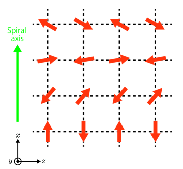
Figure 1: Schematic illustration of the magnetic structure of the screw-type spiral magnet. The red arrows represent the spins. The spin alignment in a $x$ direction is spiral, and that in a $z$ direction is antiferromagnetic; because of this, we call a $x$ axis a spiral axis, which is represented by a green arrow.

To describe magnon properties of $\hat{H}_{0}$, we express $\hat{H}_{0}$ in terms of magnon operators by using the linear-spin-wave approximation. For the details of the linear-spin-wave approximation for a noncollinear magnet, see Refs. Gingras, , Toth, and NA-pyro, . First, we introduce a rotation matrix, defined as follows:

$$\langle\hat{\bm{S}}_{\bm{i}}\rangle=R_{\bm{i}}\langle\hat{\bm{S}}^{\prime}_{\bm{i}}\rangle,$$ (12)

where $\langle\hat{\bm{S}}^{\prime}_{\bm{i}}\rangle={}^{t}(0\ 0\ S)$. We have introduced this matrix because the Holstein-Primakoff transformation for a collinear ferromagnet is applicable to $\hat{H}_{0}$ expressed in terms of $\hat{\bm{S}}^{\prime}_{\bm{i}}$. For the screw-type spiral magnet, $R_{\bm{i}}$ is

$$R_{\bm{i}}=\left(\begin{array}[]{@{\,}ccc@{\,}}\cos(\bm{Q}\cdot\bm{i})&0&\sin(\bm{Q}\cdot\bm{i})\\ 0&1&0\\ -\sin(\bm{Q}\cdot\bm{i})&0&\cos(\bm{Q}\cdot\bm{i})\end{array}\right).$$ (16)

By using this rotation matrix, we obtain the following relation between the spin operators:

$$\hat{S}_{\bm{i}}^{x}=\cos(\bm{Q}\cdot\bm{i})\hat{S}_{\bm{i}}^{\prime x}+\sin(\bm{Q}\cdot\bm{i})\hat{S}_{\bm{i}}^{\prime z},$$ (17)

$$\hat{S}_{\bm{i}}^{y}=\hat{S}_{\bm{i}}^{\prime y},$$ (18)

$$\hat{S}_{\bm{i}}^{z}=-\sin(\bm{Q}\cdot\bm{i})\hat{S}_{\bm{i}}^{\prime x}+\cos(\bm{Q}\cdot\bm{i})\hat{S}_{\bm{i}}^{\prime z}.$$ (19)

Second, by using Eqs. (17)–(19), we express $\hat{H}_{0}$ in terms of $\hat{\bm{S}}_{\bm{i}}^{\prime}$. As a result, we obtain

$$\hat{H}_{0}= -\sum\limits_{\langle\bm{i},\bm{j}\rangle}\tilde{J}_{\bm{i}\bm{j}}(\hat{S}_{\bm{i}}^{\prime x}\hat{S}_{\bm{j}}^{\prime x}+\hat{S}_{\bm{i}}^{\prime z}\hat{S}_{\bm{j}}^{\prime z})+\sum\limits_{\langle\bm{i},\bm{j}\rangle}J_{\bm{i}\bm{j}}\hat{S}_{\bm{i}}^{\prime y}\hat{S}_{\bm{j}}^{\prime y},$$ (20)

where

$$\tilde{J}_{\bm{i}\bm{j}}=\begin{cases}\sqrt{J^{2}+D^{2}}\ \ (|j_{x}-i_{x}|=1,\ i_{z}=j_{z}),\\ J\ \ \ \ \ \ \ \ \ \ \ \ \ (|j_{z}-i_{z}|=1,\ i_{x}=j_{x}),\\ 0\ \ \ \ \ \ \ \ \ \ \ \ \ \ (\textrm{otherwise}).\end{cases}$$ (21)

The details of this derivation are described in Appendix C. Third, we express $\hat{H}_{0}$ in terms of magnon operators by using the Holstein-Primakoff transformation, which connects spin operators and magnon operators as follows:

$$\hat{S}_{\bm{i}}^{\prime z}=S-\hat{b}^{\dagger}_{\bm{i}}\hat{b}_{\bm{i}},$$ (22)

$$\hat{S}_{\bm{i}}^{\prime x}=\sqrt{\frac{S}{2}}(\hat{b}_{\bm{i}}+\hat{b}_{\bm{i}}^{\dagger}),$$ (23)

$$\hat{S}_{\bm{i}}^{\prime y}=-i\sqrt{\frac{S}{2}}(\hat{b}_{\bm{i}}-\hat{b}_{\bm{i}}^{\dagger}),$$ (24)

where $\hat{b}^{\dagger}_{\bm{i}}$ and $\hat{b}_{\bm{i}}$ are creation and annihilation operators of a magnon. (Because of this transformation, the vectorial nature of spin waves, which are characterized as $\Delta\hat{\bm{S}}_{\bm{i}}^{\prime}=\hat{\bm{S}}_{\bm{i}}^{\prime}-\langle\hat{\bm{S}}_{\bm{i}}^{\prime}\rangle$, can be taken into account in the theory using the magnon operators.) Since only the quadratic terms of magnon operators are considered in the linear-spin-wave approximation, the magnon Hamiltonian without impurities for the screw-type spiral magnet in the linear-spin-wave approximation is given by

$$\hat{H}_{0}= S\sum\limits_{\langle\bm{i},\bm{j}\rangle}\tilde{J}_{\bm{i}\bm{j}}(\hat{b}_{\bm{i}}^{\dagger}\hat{b}_{\bm{i}}+\hat{b}_{\bm{j}}^{\dagger}\hat{b}_{\bm{j}})-\frac{S}{2}\sum\limits_{\langle\bm{i},\bm{j}\rangle}\tilde{J}_{\bm{i}\bm{j}}^{(+)}(\hat{b}_{\bm{i}}\hat{b}_{\bm{j}}+\hat{b}_{\bm{i}}^{\dagger}\hat{b}_{\bm{j}}^{\dagger})$$

$$-\frac{S}{2}\sum\limits_{\langle\bm{i},\bm{j}\rangle}\tilde{J}_{\bm{i}\bm{j}}^{(-)}(\hat{b}_{\bm{i}}^{\dagger}\hat{b}_{\bm{j}}+\hat{b}_{\bm{i}}\hat{b}_{\bm{j}}^{\dagger}),$$ (25)

where $\tilde{J}_{\bm{i}\bm{j}}^{(\pm)}=\tilde{J}_{\bm{i}\bm{j}}\pm J_{\bm{i}\bm{j}}$.

Then we can obtain the energy dispersion relation of magnon bands for our spiral magnet by using the Fourier transformations and the Bogoliubov transformation. By using the Fourier transformations of the magnon operators in Eq. (25), e.g., $\hat{b}_{\bm{i}}=\frac{1}{\sqrt{N}}\sum{}_{\bm{q}}\hat{b}_{\bm{q}}e^{-i\bm{q}\cdot\bm{i}}$, we obtain

$$\hat{H}_{0}= \sum\limits_{\bm{q}}A(\bm{q})(\hat{b}_{\bm{q}}^{\dagger}\hat{b}_{\bm{q}}+\hat{b}_{-\bm{q}}\hat{b}_{-\bm{q}}^{\dagger})+\sum\limits_{\bm{q}}B(\bm{q})(\hat{b}_{-\bm{q}}\hat{b}_{\bm{q}}+\hat{b}_{\bm{q}}^{\dagger}\hat{b}_{-\bm{q}}^{\dagger})$$

$$= \sum\limits_{\bm{q}}\left(\hat{b}^{\dagger}_{\bm{q}}\ \hat{b}_{-\bm{q}}\right)\left(\begin{array}[]{@{\,}cc@{\,}}A(\bm{q})&B(\bm{q})\\ B(\bm{q})&A(\bm{q})\end{array}\right)\left(\begin{array}[]{@{\,}c@{\,}}\hat{b}_{\bm{q}}\\ \hat{b}_{-\bm{q}}^{\dagger}\end{array}\right).$$ (30)

Here

$$A(\bm{q})=\frac{S}{2}\tilde{J}(\bm{0})-\frac{S}{4}\tilde{J}^{(-)}(\bm{q}),$$ (31)

$$B(\bm{q})=-\frac{S}{4}\tilde{J}^{(+)}(\bm{q}),$$ (32)

where $\tilde{J}(\bm{0})=\sum_{j=1}^{z}\tilde{J}_{\bm{r}_{i}\bm{r}_{j}}$ and $\tilde{J}^{(\pm)}(\bm{q})=\sum_{j=1}^{z}\tilde{J}_{\bm{r}_{i}\bm{r}_{j}}^{(\pm)}e^{i\bm{q}\cdot(\bm{r}_{i}-\bm{r}_{j})}$, with $z$, the coordination number. Equation (30) can be also expressed as follows:

$$\hat{H}_{0}=\sum\limits_{\bm{q}}\sum\limits_{a,b=1,2}H_{ab}(\bm{q})\hat{x}_{\bm{q}a}^{\dagger}\hat{x}_{\bm{q}b},$$ (33)

where $\hat{x}_{\bm{q}1}=\hat{b}_{\bm{q}}$, $\hat{x}_{\bm{q}2}=\hat{b}_{-\bm{q}}^{\dagger}$, $H_{11}(\bm{q})=H_{22}(\bm{q})=A(\bm{q})$, and $H_{12}(\bm{q})=H_{21}(\bm{q})=B(\bm{q})$. We can diagonalize Eq. (30) by using the Bogoliubov transformation,

$$\left(\begin{array}[]{@{\,}c@{\,}}\hat{b}_{\bm{q}}\\ \hat{b}_{-\bm{q}}^{\dagger}\end{array}\right)=\left(\begin{array}[]{@{\,}cc@{\,}}\cosh\theta_{\bm{q}}&-\sinh\theta_{\bm{q}}\\ -\sinh\theta_{\bm{q}}&\cosh\theta_{\bm{q}}\end{array}\right)\left(\begin{array}[]{@{\,}c@{\,}}\hat{\gamma}_{\bm{q}}\\ \hat{\gamma}_{-\bm{q}}^{\dagger}\end{array}\right),$$ (40)

where the hyperbolic functions are determined by

$$\tanh 2\theta_{\bm{q}}=\frac{B(\bm{q})}{A(\bm{q})}.$$ (41)

The diagonalized Hamiltonian is given by

$$\hat{H}_{0}= \frac{1}{2}\sum\limits_{\bm{q}}\epsilon(\bm{q})(\hat{\gamma}_{\bm{q}}^{\dagger}\hat{\gamma}_{\bm{q}}+\hat{\gamma}_{-\bm{q}}\hat{\gamma}_{-\bm{q}}^{\dagger})$$

$$= \frac{1}{2}\sum\limits_{\bm{q}}\left(\hat{\gamma}^{\dagger}_{\bm{q}}\ \hat{\gamma}_{-\bm{q}}\right)\left(\begin{array}[]{@{\,}cc@{\,}}\epsilon(\bm{q})&0\\ 0&\epsilon(\bm{q})\end{array}\right)\left(\begin{array}[]{@{\,}c@{\,}}\hat{\gamma}_{\bm{q}}\\ \hat{\gamma}_{-\bm{q}}^{\dagger}\end{array}\right),$$ (46)

where

$$\epsilon(\bm{q})=2\sqrt{A(\bm{q})^{2}-B(\bm{q})^{2}}.$$ (47)

The most important property of the energy dispersion relation is the degeneracy of magnon bands because this degeneracy results from global time-reversal symmetry remark2 ; a similar degeneracy exists in a collinear antiferromagnet Lett . (This degeneracy is similar to the Kramers degeneracy in an electron system with time-reversal symmetry.) For other important properties, see Appendix D.

II.2 $\hat{H}_{\textrm{imp}}$

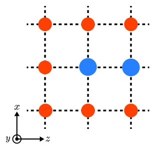
Figure 2: Schematic illustration of our disordered system. The orange circles represent original magnetic ions, and the blue circles represent impurities, which are introduced by substituting part of the original magnetic ions by different ones.

We construct $\hat{H}_{\textrm{imp}}$ in a similar way to the disordered antiferromagnet Lett ; Full . We introduce impurities into the screw-type spiral magnet by substituting part of the magnetic ions by different ones, which belong to the same family in the periodic table; our disordered system is schematically illustrated in Fig. 2. We have considered such a partial substitution because the magnetic ions in the same family have the same $S$ and because its main effect is to modify the values of exchange interactions Lett ; Full . For our spiral magnet, described by Eq. (20), such a modification can be described as the following spin Hamiltonian:

$$\hat{H}_{\textrm{imp}}= -\sum\limits_{\langle\bm{i},\bm{j}\rangle}\Delta\tilde{J}_{\bm{i}\bm{j}}(\hat{S}_{\bm{i}}^{\prime x}\hat{S}_{\bm{j}}^{\prime x}+\hat{S}_{\bm{i}}^{\prime z}\hat{S}_{\bm{j}}^{\prime z})+\sum\limits_{\langle\bm{i},\bm{j}\rangle}\Delta J_{\bm{i}\bm{j}}\hat{S}_{\bm{i}}^{\prime y}\hat{S}_{\bm{j}}^{\prime y},$$ (48)

where

$$\Delta\tilde{J}_{\bm{i}\bm{j}}=\begin{cases}\tilde{J}^{\prime}_{\bm{i}\bm{j}}\ \ \ \ (\bm{i}\in N_{0},\ \bm{j}\in N_{\textrm{imp}}),\\ \tilde{J}^{\prime}_{\bm{i}\bm{j}}\ \ \ \ (\bm{i}\in N_{\textrm{imp}},\ \bm{j}\in N_{0}),\\ \tilde{J}^{\prime\prime}_{\bm{i}\bm{j}}\ \ \ \ (\bm{i},\bm{j}\in N_{\textrm{imp}}),\\ 0\ \ \ \ \ \ (\textrm{otherwise}),\end{cases}$$ (49)

$$\Delta J_{\bm{i}\bm{j}}=\begin{cases}J^{\prime}\ \ \ \ (\bm{i}\in N_{0},\ \bm{j}\in N_{\textrm{imp}}),\\ J^{\prime}\ \ \ \ (\bm{i}\in N_{\textrm{imp}},\ \bm{j}\in N_{0}),\\ J^{\prime\prime}\ \ \ \ (\bm{i},\bm{j}\in N_{\textrm{imp}}),\\ 0\ \ \ \ \ \ (\textrm{otherwise}),\end{cases}$$ (50)

with

$$\tilde{J}^{\prime}_{\bm{i}\bm{j}}=\begin{cases}\sqrt{(J^{\prime})^{2}+(D^{\prime})^{2}}\ \ (|j_{x}-i_{x}|=1,\ i_{z}=j_{z}),\\ J^{\prime}\ \ \ \ \ \ \ \ \ \ \ \ \ \ \ \ \ \ \ \ (|j_{z}-i_{z}|=1,\ i_{x}=j_{x}),\\ 0\ \ \ \ \ \ \ \ \ \ \ \ \ \ \ \ \ \ \ \ \ (\textrm{otherwise}),\end{cases}$$ (51)

$$\tilde{J}^{\prime\prime}_{\bm{i}\bm{j}}=\begin{cases}\sqrt{(J^{\prime\prime})^{2}+(D^{\prime\prime})^{2}}\ \ (|j_{x}-i_{x}|=1,\ i_{z}=j_{z}),\\ J^{\prime\prime}\ \ \ \ \ \ \ \ \ \ \ \ \ \ \ \ \ \ \ \ (|j_{z}-i_{z}|=1,\ i_{x}=j_{x}),\\ 0\ \ \ \ \ \ \ \ \ \ \ \ \ \ \ \ \ \ \ \ \ \ (\textrm{otherwise}).\end{cases}$$ (52)

In Eqs. (49) and (50) $N_{0}$ represents the nonsubstituted magnetic ions (i.e., orange circles in Fig. 2) and $N_{\textrm{imp}}$ represents the impurities (i.e., blue circles in Fig. 2). We assume that $J^{\prime}$ and $J^{\prime\prime}$ are much smaller than $J$, and that $D^{\prime}$ and $D^{\prime\prime}$ are much smaller than $D$. Owing to these assumptions, the effects of $\hat{H}_{\textrm{imp}}$ can be treated as perturbation; under these assumptions the effects of $J^{\prime}$, $J^{\prime\prime}$, $D^{\prime}$, and $D^{\prime\prime}$ on the spin-spiral angle, $\bm{Q}\cdot\bm{i}$ of $\langle\bm{S}_{\bm{i}}\rangle$, are negligible. In addition, since the dominant terms of Eq. (48) come from the mean-field terms and magnetic ions in the same family in the periodic table have the same $S$, $\hat{H}_{\textrm{imp}}$ can be approximated as follows:

$$\hat{H}_{\textrm{imp}}=-2\sum\limits_{\bm{j}\in N}V\hat{S}_{\bm{j}}^{\prime z}-2\sum\limits_{\bm{j}\in N_{\textrm{imp}}}V^{(\textrm{imp})}\hat{S}_{\bm{j}}^{\prime z},$$ (53)

where $\sum_{\bm{j}\in N}$ is the summation for all sites, and $\sum_{\bm{j}\in N_{\textrm{imp}}}$ is the summation for impurity sites; $V=(Sz^{\prime}/2)[\sqrt{(J^{\prime})^{2}+(D^{\prime})^{2}}+J^{\prime}]$ and $V^{(\textrm{imp})}=(Sz^{\prime\prime}/2)[\sqrt{(J^{\prime\prime})^{2}+(D^{\prime\prime})^{2}}+J^{\prime\prime}]$, where $z^{\prime}$ and $z^{\prime\prime}$ are the coordination numbers for $\Delta\tilde{J}_{\bm{i}\bm{j}}=\tilde{J}_{\bm{i}\bm{j}}^{\prime}$ and $\tilde{J}_{\bm{i}\bm{j}}^{\prime\prime}$, respectively. In the derivation of Eq. (53) we have used $\langle\hat{\bm{S}}_{\bm{i}}^{\prime}\rangle={}^{t}(0\ 0\ S)$. In a similar way to $\hat{H}_{0}$, we can express $\hat{H}_{\textrm{imp}}$ in terms of magnon operators:

$$\hat{H}_{\textrm{imp}}=2\sum\limits_{\bm{q}}V\hat{b}_{\bm{q}}^{\dagger}\hat{b}_{\bm{q}}+2\sum\limits_{\bm{q},\bm{q}^{\prime}}V^{(\textrm{imp})}(\bm{q}-\bm{q}^{\prime})\hat{b}_{\bm{q}}^{\dagger}\hat{b}_{\bm{q}^{\prime}},$$ (54)

where

$$V^{(\textrm{imp})}(\bm{q}-\bm{q}^{\prime})=\frac{1}{N}\sum\limits_{\bm{j}\in N_{\textrm{imp}}}V^{(\textrm{imp})}e^{i(\bm{q}-\bm{q}^{\prime})\cdot\bm{j}}.$$ (55)

In the following analyses we neglect the first term of Eq. (54) for simplicity because its effect is a small, uniform shift of the diagonal terms of $\hat{H}_{0}$ in Eq. (30), i.e., shifting $A(\bm{q})$ into $A(\bm{q})+V$. We thus use the following as the Hamiltonian of impurities:

$$\hat{H}_{\textrm{imp}}= 2\sum\limits_{\bm{q},\bm{q}^{\prime}}V^{(\textrm{imp})}(\bm{q}-\bm{q}^{\prime})\hat{b}_{\bm{q}}^{\dagger}\hat{b}_{\bm{q}^{\prime}}$$

$$= \sum\limits_{\bm{q},\bm{q}^{\prime}}\sum\limits_{a=1,2}V^{(\textrm{imp})}(\bm{q}-\bm{q}^{\prime})\hat{x}_{\bm{q}a}^{\dagger}\hat{x}_{\bm{q}^{\prime}a}.$$ (56)

III Linear-response theory

To analyze magnon transport of the disordered spiral magnet, we consider longitudinal thermal conductivities under local equilibrium with local energy conservation. A longitudinal thermal conductivity, $\kappa_{\alpha\alpha}$, is defined as $j_{E}^{\alpha}=\kappa_{\alpha\alpha}(-\partial_{\alpha}T)$, where $(-\partial_{\alpha}T)$ is the temperature gradient along the $\alpha$ axis, and $j_{E}^{\alpha}$ is the density of the energy current parallel to the temperature gradient. This conductivity is suitable for analyses of the weak localization of magnons in the presence of global time-reversal symmetry because this can be finite even with global time-reversal symmetry. (Note that other conductivities, such as the thermal Hall conductivity, are not suitable because those can be zero at finite temperatures even without impurities.) Because of the local equilibrium, the local temperature can be defined. Then, because of the local energy conservation, the energy current operator can be derived from the following equation Mahan-text :

$$\hat{\bm{J}}_{E}=i\sum\limits_{\bm{m},\bm{n}}\bm{r}_{\bm{n}}[\hat{h}_{\bm{m}},\hat{h}_{\bm{n}}],$$ (57)

where $\hat{h}_{\bm{j}}$ is given by $\hat{H}=\sum_{\bm{j}}\hat{h}_{\bm{j}}$. By calculating the right-hand side of Eq. (57) for $\hat{H}=\hat{H}_{0}$, we obtain the energy current operator of a magnon for our disordered spiral magnet,

$$\hat{\bm{J}}_{E}=\sum\limits_{\bm{q}}\sum\limits_{a,b=1,2}\hat{x}^{\dagger}_{\bm{q}a}\bm{e}_{ab}(\bm{q})\hat{x}_{\bm{q}b},$$ (58)

where

$$\bm{e}_{11}(\bm{q})=-\bm{e}_{22}(\bm{q})=2\frac{\partial B(\bm{q})}{\partial\bm{q}}B(\bm{q})-2\frac{\partial A(\bm{q})}{\partial\bm{q}}A(\bm{q}),$$ (59)

$$\bm{e}_{12}(\bm{q})=\bm{e}_{21}(\bm{q})=-2\frac{\partial B(\bm{q})}{\partial\bm{q}}A(\bm{q})-2\frac{\partial A(\bm{q})}{\partial\bm{q}}B(\bm{q}).$$ (60)

The details of this derivation are described in Appendix E. For the energy current operator we have neglected the terms due to the combination of $\hat{H}_{0}$ and $\hat{H}_{\textrm{imp}}$ because in the weak-localization regime these terms will be negligible compared with the terms of Eq. (58).

By using the linear-response theory for $\kappa_{\alpha\alpha}$, we can express $\kappa_{\alpha\alpha}$ as follows:

$$\kappa_{\alpha\alpha}=\frac{1}{T}\lim\limits_{\omega\rightarrow 0}\dfrac{K_{\alpha\alpha}^{(\textrm{R})}(\omega)-K_{\alpha\alpha}^{(\textrm{R})}(0)}{i\omega},$$ (61)

where $K_{\alpha\alpha}^{(\textrm{R})}(\omega)=K_{\alpha\alpha}(i\Omega_{n}\rightarrow\omega+i0+)$, with $\Omega_{n}=2\pi Tn$ $(n=0,\pm 1,\cdots)$ and

$$K_{\alpha\alpha}(i\Omega_{n})=\frac{1}{N}\int^{T^{-1}}_{0}d\tau e^{i\Omega_{n}\tau}\langle\textrm{T}_{\tau}\hat{J}_{\textrm{E}}^{\alpha}(\tau)\hat{J}_{\textrm{E}}^{\alpha}\rangle.$$ (62)

Substituting Eq. (58) into Eq. (62) and using a technique of the quantum field theory AGD ; Eliashberg ; NA-Ch , we can express $K_{\alpha\alpha}(i\Omega_{n})$ in terms of magnon Green’s functions:

$$K_{\alpha\alpha}(i\Omega_{n})=\frac{1}{N}\sum\limits_{\bm{q},\bm{q}^{\prime}}\sum\limits_{a,b,c,d}e_{ab}^{\alpha}(\bm{q})e_{cd}^{\alpha}(\bm{q}^{\prime})$$

$$\times T\sum\limits_{m}\langle D_{da}(\bm{q}^{\prime},\bm{q},i\Omega_{m})D_{bc}(\bm{q},\bm{q}^{\prime},i\Omega_{m}+i\Omega_{n})\rangle,$$ (63)

where $D_{ab}(\bm{q},\bm{q}^{\prime},i\Omega_{m})$ is the Green’s function of a magnon in the Matsubara-frequency representation before taking the impurity averaging. Then, by calculating the summation over the Matsubara frequency in Eq. (63) and carrying out the analytic continuation (i.e., $i\Omega_{n}\rightarrow\omega+i0+$), $\kappa_{\alpha\alpha}$ can be expressed as follows:

$$\kappa_{\alpha\alpha}= \frac{1}{TN}\sum\limits_{\bm{q},\bm{q}^{\prime}}\sum\limits_{a,b,c,d}e_{ab}^{\alpha}(\bm{q})e_{cd}^{\alpha}(\bm{q}^{\prime})P\int_{-\infty}^{\infty}\frac{d\epsilon}{2\pi}\Bigl{[}-\frac{\partial n(\epsilon)}{\partial\epsilon}\Bigr{]}$$

$$\times\Bigl{[}\langle D^{(\textrm{A})}_{da}(\bm{q}^{\prime},\bm{q},\epsilon)D^{(\textrm{R})}_{bc}(\bm{q},\bm{q}^{\prime},\epsilon)\rangle$$

$$\ \ \ \ -\frac{1}{2}\langle D^{(\textrm{R})}_{da}(\bm{q}^{\prime},\bm{q},\epsilon)D^{(\textrm{R})}_{bc}(\bm{q},\bm{q}^{\prime},\epsilon)\rangle$$

$$\ \ \ \ -\frac{1}{2}\langle D^{(\textrm{A})}_{da}(\bm{q}^{\prime},\bm{q},\epsilon)D^{(\textrm{A})}_{bc}(\bm{q},\bm{q}^{\prime},\epsilon)\rangle\Bigr{]}.$$ (64)

Here $n(\epsilon)=(e^{\epsilon/T}-1)$ is the Bose distribution function; $D^{(\textrm{R})}_{ab}(\bm{q},\bm{q}^{\prime},\epsilon)$ and $D^{(\textrm{A})}_{ab}(\bm{q},\bm{q}^{\prime},\epsilon)$ are the retarded and advanced Green’s functions in the real-frequency representation before taking the impurity averaging. Equation (64) provides a starting point for formulating an approximate theory in the weak-localization regime.

IV Weak-localization theory

We formulate the weak-localization theory for magnons of our disordered spiral magnet. The weak-localization theory is an approximate theory in the weak-localization regime because this takes account of the main effect of impurities Berg ; Nagaoka ; Lett in the weak-localization regime. Since in Eq. (64) the main contribution in the weak-localization regime comes from the term including $\langle D^{(\textrm{A})}_{da}(\bm{q}^{\prime},\bm{q},\epsilon)D^{(\textrm{R})}_{bc}(\bm{q},\bm{q}^{\prime},\epsilon)\rangle$ Berg ; Nagaoka ; Lett , $\kappa_{\alpha\alpha}$ can be approximated as follows:

$$\kappa_{\alpha\alpha}= \frac{1}{TN}\sum\limits_{\bm{q},\bm{q}^{\prime}}\sum\limits_{a,b,c,d}e_{ab}^{\alpha}(\bm{q})e_{cd}^{\alpha}(\bm{q}^{\prime})P\int_{-\infty}^{\infty}\frac{d\epsilon}{2\pi}\Bigl{[}-\frac{\partial n(\epsilon)}{\partial\epsilon}\Bigr{]}$$

$$\times\langle D^{(\textrm{A})}_{da}(\bm{q}^{\prime},\bm{q},\epsilon)D^{(\textrm{R})}_{bc}(\bm{q},\bm{q}^{\prime},\epsilon)\rangle.$$ (65)

Then, by carrying out the perturbation expansions for the magnon Green’s functions in Eq. (65), taking the impurity averaging, and considering only the dominant terms, $\kappa_{\alpha\alpha}$ can be expressed as follows:

$$\kappa_{\alpha\alpha}=\kappa_{\alpha\alpha}^{(\textrm{Born})}+\Delta\kappa_{\alpha\alpha},$$ (66)

where $\kappa_{\alpha\alpha}^{(\textrm{Born})}$ is the term in the Born approximation,

$$\kappa_{\alpha\alpha}^{(\textrm{Born})}= \frac{1}{TN}\sum\limits_{\bm{q}}\sum\limits_{a,b,c,d}e_{ab}^{\alpha}(\bm{q})e_{cd}^{\alpha}(\bm{q})P\int_{-\infty}^{\infty}\frac{d\epsilon}{2\pi}\Bigl{[}-\frac{\partial n(\epsilon)}{\partial\epsilon}\Bigr{]}$$

$$\times\bar{D}^{(\textrm{A})}_{da}(\bm{q},\epsilon)\bar{D}^{(\textrm{R})}_{bc}(\bm{q},\epsilon),$$ (67)

and $\Delta\kappa_{\alpha\alpha}$ is the main correction term in the weak-localization regime,

$$\Delta\kappa_{\alpha\alpha}= \frac{1}{TN}\sum\limits_{\bm{q},\bm{q}^{\prime}}\sum\limits_{a,b,c,d}e_{ab}^{\alpha}(\bm{q})e_{cd}^{\alpha}(\bm{q}^{\prime})P\int_{-\infty}^{\infty}\frac{d\epsilon}{2\pi}\Bigl{[}-\frac{\partial n(\epsilon)}{\partial\epsilon}\Bigr{]}$$

$$\times\sum\limits_{a^{\prime},b^{\prime},c^{\prime},d^{\prime}}\bar{D}^{(\textrm{A})}_{dd^{\prime}}(\bm{q}^{\prime},\epsilon)\bar{D}^{(\textrm{A})}_{a^{\prime}a}(\bm{q},\epsilon)\Gamma_{a^{\prime}b^{\prime}c^{\prime}d^{\prime}}(\bm{q}+\bm{q}^{\prime},\epsilon)$$

$$\times\bar{D}^{(\textrm{R})}_{bb^{\prime}}(\bm{q},\epsilon)\bar{D}^{(\textrm{R})}_{c^{\prime}c}(\bm{q}^{\prime},\epsilon).$$ (68)

We have introduced the following quantities: $\bar{D}^{(\textrm{R})}_{ab}(\bm{q},\epsilon)$ and $\bar{D}^{(\textrm{A})}_{ab}(\bm{q},\epsilon)$ are the retarded and advanced Green’s functions after taking the impurity averaging; $\Gamma_{abcd}(\bm{Q},\epsilon)$ is the particle-particle type four-point vertex function. These Green’s functions are determined from the Dyson equation for the self-energy in the Born approximation; for example, $\bar{D}^{(\textrm{R})}_{ab}(\bm{q},\epsilon)$ is given by

$$\bar{D}^{(\textrm{R})}_{ab}(\bm{q},\epsilon)= D^{0(\textrm{R})}_{ab}(\bm{q},\epsilon)$$

$$+\sum\limits_{a^{\prime},b^{\prime}}D^{0(\textrm{R})}_{aa^{\prime}}(\bm{q},\epsilon)\Sigma_{a^{\prime}b^{\prime}}^{(\textrm{R})}(\epsilon)\bar{D}^{(\textrm{R})}_{b^{\prime}b}(\bm{q},\epsilon),$$ (69)

with

$$D^{0(\textrm{R})}_{ab}(\bm{q},\epsilon)=\dfrac{U_{a\alpha}(\bm{q})U_{b\alpha}(\bm{q})}{\epsilon-\epsilon(\bm{q})+i\delta}-\dfrac{U_{a\beta}(\bm{q})U_{b\beta}(\bm{q})}{\epsilon+\epsilon(\bm{q})+i\delta},$$ (70)

$$\Sigma_{ab}^{(\textrm{R})}(\epsilon)=\dfrac{n_{\textrm{imp}}V_{\textrm{imp}}^{2}}{N}\sum\limits_{\bm{q}}\bar{D}^{(\textrm{R})}_{ab}(\bm{q},\epsilon),$$ (71)

where $\delta=0+$, $U_{1\alpha}(\bm{q})=U_{2\beta}(\bm{q})=\cosh\theta_{\bm{q}}$, $U_{1\beta}(\bm{q})=U_{2\alpha}(\bm{q})=-\sinh\theta_{\bm{q}}$, and $n_{\textrm{imp}}$ is the impurity concentration. In addition, $\Gamma_{abcd}(\bm{Q},\epsilon)$ is determined from the following Bethe-Salpeter equation:

$$\Gamma_{abcd}(\bm{Q},\epsilon)= \gamma_{\textrm{imp}}^{2}\Pi_{abcd}(\bm{Q},\epsilon)$$

$$+\sum\limits_{e,f}\gamma_{\textrm{imp}}\Pi_{aecf}(\bm{Q},\epsilon)\Gamma_{fbed}(\bm{Q},\epsilon),$$ (72)

where $\gamma_{\textrm{imp}}=\frac{n_{\textrm{imp}}V_{\textrm{imp}}^{2}}{N}$ and

$$\Pi_{abcd}(\bm{Q},\epsilon)=\sum\limits_{\bm{q}_{1}}\bar{D}^{(\textrm{R})}_{bc}(\bm{q}_{1},\epsilon)\bar{D}^{(\textrm{A})}_{da}(\bm{Q}-\bm{q}_{1},\epsilon).$$ (73)

Then we introduce two simplifications. One is to neglect the real part of the self-energy, i.e., consider only the imaginary part; as a result,

$$\Sigma_{ab}^{(\textrm{R})}(\epsilon)=-i\gamma_{ab}(\epsilon),$$ (74)

$$\Sigma_{ab}^{(\textrm{A})}(\epsilon)=i\gamma_{ab}(\epsilon),$$ (75)

where

$$\gamma_{ab}(\epsilon)=-\gamma_{\textrm{imp}}\sum\limits_{\bm{q}}\textrm{Im}\bar{D}_{ab}^{(\textrm{R})}(\bm{q},\epsilon).$$ (76)

The other is to approximate $D^{0(\textrm{R})}_{ab}(\bm{q},\epsilon)$ and $D^{0(\textrm{A})}_{ab}(\bm{q},\epsilon)$ as follows:

$$D^{0(\textrm{R})}_{ab}(\bm{q},\epsilon)\sim\begin{cases}\dfrac{U_{a\alpha}(\bm{q})U_{b\alpha}(\bm{q})}{\epsilon-\epsilon_{\bm{q}}+i\delta}\ \ (\epsilon>0),\\[6.0pt] -\dfrac{U_{a\beta}(\bm{q})U_{b\beta}(\bm{q})}{\epsilon+\epsilon_{\bm{q}}+i\delta}\ (\epsilon<0),\end{cases}$$ (77)

$$D^{0(\textrm{A})}_{ab}(\bm{q},\epsilon)\sim\begin{cases}\dfrac{U_{a\alpha}(\bm{q})U_{b\alpha}(\bm{q})}{\epsilon-\epsilon_{\bm{q}}-i\delta}\ \ (\epsilon>0),\\[6.0pt] -\dfrac{U_{a\beta}(\bm{q})U_{b\beta}(\bm{q})}{\epsilon+\epsilon_{\bm{q}}-i\delta}\ (\epsilon<0).\end{cases}$$ (78)

These simplifications, which are similar to those for the disordered antiferromagnet Lett , will be appropriate for a rough estimate of the main effect of impurities because the imaginary part of the self-energy is vital for the weak localization Berg ; Nagaoka ; Lett , and because the main contribution to $D^{0(\textrm{R})}_{ab}(\bm{q},\epsilon)$ for $\epsilon>0$ or $\epsilon<0$ comes from the first or second term, respectively, of Eq. (70).

By using the above two simplifications, we can obtain the approximate expressions of $\bar{D}^{(\textrm{R})}_{ab}(\bm{q},\epsilon)$, $\bar{D}^{(\textrm{A})}_{ab}(\bm{q},\epsilon)$, $\Pi_{abcd}(\bm{Q},\epsilon)$, and $\Gamma_{abcd}(\bm{Q},\epsilon)$. First, by combining the simplifications with the Dyson equation, $\bar{D}^{(\textrm{R})}_{ab}(\bm{q},\epsilon)$ and $\bar{D}^{(\textrm{A})}_{ab}(\bm{q},\epsilon)$ can be expressed as follows:

$$\bar{D}^{(\textrm{R})}_{ab}(\bm{q},\epsilon)\sim\begin{cases}\dfrac{U_{a\alpha}(\bm{q})U_{b\alpha}(\bm{q})}{\epsilon-\epsilon(\bm{q})+i\tilde{\gamma}(\epsilon)}\ \ \ \ \ \ (\epsilon>0),\\[6.0pt] -\dfrac{U_{a\beta}(\bm{q})U_{b\beta}(\bm{q})}{\epsilon+\epsilon(\bm{q})+i\tilde{\gamma}(-\epsilon)}\ (\epsilon<0),\end{cases}$$ (79)

$$\bar{D}^{(\textrm{A})}_{ab}(\bm{q},\epsilon)\sim\begin{cases}\dfrac{U_{a\alpha}(\bm{q})U_{b\alpha}(\bm{q})}{\epsilon-\epsilon(\bm{q})-i\tilde{\gamma}(\epsilon)}\ \ \ \ \ \ (\epsilon>0),\\[6.0pt] -\dfrac{U_{a\beta}(\bm{q})U_{b\beta}(\bm{q})}{\epsilon+\epsilon(\bm{q})-i\tilde{\gamma}(-\epsilon)}\ (\epsilon<0).\end{cases}$$ (80)

with

$$\tilde{\gamma}(\epsilon)= (\cosh^{2}\theta_{\bm{q}}+\sinh^{2}\theta_{\bm{q}})^{2}\gamma(\epsilon)$$

$$= (\cosh^{2}\theta_{\bm{q}}+\sinh^{2}\theta_{\bm{q}})^{2}\pi n_{\textrm{imp}}V_{\textrm{imp}}^{2}\rho(\epsilon),$$ (81)

where $\bm{q}$ of $\cosh^{2}\theta_{\bm{q}}$ and $\sinh^{2}\theta_{\bm{q}}$ are determined by $\epsilon(\bm{q})=|\epsilon|$, and $\rho(\epsilon)$ is the density of states. Second, by substituting Eqs. (79) and (80) into Eq. (73) and performing the calculations described in Appendix F, we can express $\Pi_{abcd}(\bm{Q},\epsilon)$ for small $Q=|\bm{Q}|$ as follows:

$$\Pi_{abcd}(\bm{Q},\epsilon)$$

$$\sim\begin{cases}\dfrac{u_{b\alpha}u_{c\alpha}u_{d\alpha}u_{a\alpha}}{\gamma_{\textrm{imp}}(c_{0}^{2}+s_{0}^{2})^{2}}[1-D_{\textrm{S}}(\epsilon)Q^{2}\tilde{\tau}(\epsilon)]\ \ \ \ \ (\epsilon>0),\\[8.0pt] \dfrac{u_{b\beta}u_{c\beta}u_{d\beta}u_{a\beta}}{\gamma_{\textrm{imp}}(c_{0}^{2}+s_{0}^{2})^{2}}[1-D_{\textrm{S}}(-\epsilon)Q^{2}\tilde{\tau}(-\epsilon)]\ (\epsilon<0),\end{cases}$$ (82)

where $u_{a\nu}=U_{a\nu}(\bm{q}_{0})$ ($\nu=\alpha,\beta$), $c_{0}^{2}=\cosh^{2}\theta_{\bm{q}_{0}}$, $s_{0}^{2}=\sinh^{2}\theta_{\bm{q}_{0}}$, $D_{\textrm{S}}(\epsilon)=\frac{1}{8}[\frac{\partial\epsilon(\bm{q}_{0})}{\partial\bm{q}_{0}}]^{2}\tilde{\tau}(\epsilon)=\frac{1}{8}\bm{v}_{\bm{q}_{0}}^{2}\tilde{\tau}(\epsilon)$, and $\tilde{\tau}(\epsilon)=(c_{0}^{2}+s_{0}^{2})^{-2}\gamma(\epsilon)^{-1}$. In the derivation of Eq. (82) we have approximated momentum-dependent quantities, $U_{a\nu}(\bm{q}_{1})$ and $[\frac{\partial\epsilon(\bm{q}_{1})}{\partial\bm{q}_{1}}]$, as the typical values at a certain, small momentum $\bm{q}_{0}$ for a rough estimate because the dominant contributions come from the contributions for small $q_{1}=|\bm{q}_{1}|$. Note, first, that the group velocity of the magnon for $\bm{q}=\bm{0}$ is zero in our spiral magnet; second, that since the small-momentum contributions are dominant in the summation, the sum of a function $F(\bm{q})$ might be approximated by $\sum_{\bm{q}}F(\bm{q})\sim\sum_{0\leq|\bm{q}|\leq q_{\textrm{c}}}F(\bm{q})\sim F(\bm{q}_{0})\sum_{0\leq|\bm{q}|\leq q_{\textrm{c}}}$, where $q_{\textrm{c}}$ is a cut-off value. (In a rough sense this approximation is similar to a replacement of a momentum-dependent quantity in an electron system by the quantity at the Fermi momentum.) We have shown the approximate expression of $\Pi_{abcd}(\bm{Q},\epsilon)$ only for small $Q$ because the contributions for small $Q$ lead to the main contribution to $\Delta\kappa_{\alpha\alpha}$ through the diverging contribution of $\Gamma_{abcd}(\bm{Q},\epsilon)$ for $\bm{Q}=\bm{q}+\bm{q}^{\prime}$. Third, by combining Eq. (82) with Eq. (72) and solving the Bethe-Salpeter equation in the way described in Appendix G, we obtain the approximate expression of $\Gamma_{abcd}(\bm{Q},\epsilon)$ for small $Q$:

$$\Gamma_{abcd}(\bm{Q},\epsilon)\sim\begin{cases}\dfrac{u_{b\alpha}u_{c\alpha}u_{d\alpha}u_{a\alpha}\gamma_{\textrm{imp}}}{D_{\textrm{S}}(\epsilon)Q^{2}\tilde{\tau}(\epsilon)}\ \ (\epsilon>0),\\[8.0pt] \dfrac{u_{b\beta}u_{c\beta}u_{d\beta}u_{a\beta}\gamma_{\textrm{imp}}}{D_{\textrm{S}}(-\epsilon)Q^{2}\tilde{\tau}(-\epsilon)}\ \ \ (\epsilon<0).\end{cases}$$ (83)

Since $\Gamma_{abcd}(\bm{Q},\epsilon)$ diverges in the limit $Q\rightarrow 0$, the particle-particle type multiple scattering, described by $\Gamma_{abcd}(\bm{Q},\epsilon)$, for $\bm{Q}=\bm{q}+\bm{q}^{\prime}=\bm{0}$ provides the diverging contribution to $\Delta\kappa_{\alpha\alpha}$.

We can also obtain the approximate expressions of $\kappa_{\alpha\alpha}^{(\textrm{Born})}$ and $\Delta\kappa_{\alpha\alpha}$. First, by combining Eqs. (67), (59), (60), (79), and (80), we obtain

$$\kappa_{\alpha\alpha}^{(\textrm{Born})}=\frac{1}{TN}\sum\limits_{\bm{q}}\tilde{e}^{\alpha}(\bm{q})^{2}\Bigl{\{}-\frac{\partial n[\epsilon(\bm{q})]}{\partial\epsilon(\bm{q})}\Bigr{\}}\tilde{\tau}[\epsilon(\bm{q})],$$ (84)

where

$$\tilde{e}^{\alpha}(\bm{q})^{2}=e_{11}^{\alpha}(\bm{q})^{2}+e_{12}^{\alpha}(\bm{q})^{2}\sinh^{2}2\theta_{\bm{q}}.$$ (85)

In deriving Eq. (84) we have approximated $[-\frac{\partial n(\epsilon)}{\partial\epsilon}]$ and $\tilde{\tau}(\epsilon)$ as $\{-\frac{\partial n[\epsilon(\bm{q})]}{\partial\epsilon(\bm{q})}\}$ and $\tilde{\tau}[\epsilon(\bm{q})]$ because the contributions near $\epsilon=\epsilon(\bm{q})$ or $\epsilon=-\epsilon(\bm{q})$ are dominant for $\epsilon>0$ or $\epsilon<0$, respectively. Then we can obtain the approximate expression of $\Delta\kappa_{\alpha\alpha}$ in the following way. To estimate the main effect of the diverging contribution of $\Gamma_{abcd}(\bm{q}+\bm{q}^{\prime},\epsilon)$, we set $\bm{q}^{\prime}=-\bm{q}$ in Eq. (68) except for $\Gamma_{abcd}(\bm{q}+\bm{q}^{\prime},\epsilon)$ and introduce the cutoff values for the upper and lower values of the summation over $\bm{q}^{\prime}$; the lower cutoff value is $|\bm{Q}|=|\bm{q}+\bm{q}^{\prime}|=L^{-1}$, which approaches zero in the thermodynamic limit, and the upper cutoff value is $|\bm{Q}|=|\bm{q}+\bm{q}^{\prime}|=L_{\textrm{m}}^{-1}$ with the mean-free path $L_{\textrm{m}}$. As a result, $\Delta\kappa_{\alpha\alpha}$ is given by

$$\Delta\kappa_{\alpha\alpha}=-\frac{1}{TN}\sum\limits_{\bm{q}}\sum\limits_{a,b,c,d}e_{ab}^{\alpha}(\bm{q})e_{cd}^{\alpha}(\bm{q})P\int_{-\infty}^{\infty}\frac{d\epsilon}{2\pi}\Bigl{[}-\frac{\partial n(\epsilon)}{\partial\epsilon}\Bigr{]}$$

$$\times\sum\limits_{a^{\prime},b^{\prime},c^{\prime},d^{\prime}}\bar{D}_{dd^{\prime}}^{(\textrm{A})}(\bm{q},\epsilon)\bar{D}_{a^{\prime}a}^{(\textrm{A})}(\bm{q},\epsilon)\bar{D}_{bb^{\prime}}^{(\textrm{R})}(\bm{q},\epsilon)\bar{D}_{c^{\prime}c}^{(\textrm{R})}(\bm{q},\epsilon)$$

$$\times\sum\limits_{\bm{Q}}{}^{\prime}\Gamma_{a^{\prime}b^{\prime}c^{\prime}d^{\prime}}(\bm{Q},\epsilon),$$ (86)

where $\frac{1}{N}\sum_{\bm{Q}}^{\prime}=\int_{L^{-1}}^{L_{\textrm{m}}^{-1}}\frac{dq}{(2\pi)^{2}}2\pi q$. Combining Eqs. (86), (59), (60), (79), (80), and (83), we obtain

$$\Delta\kappa_{\alpha\alpha} \sim-\frac{1}{TN}\sum\limits_{\bm{q}}\tilde{e}^{\alpha}(\bm{q})^{2}\Bigl{\{}-\frac{\partial n[\epsilon(\bm{q})]}{\partial\epsilon(\bm{q})}\Bigr{\}}\tilde{\tau}[\epsilon(\bm{q})]$$

$$\times\frac{n_{\textrm{imp}}V_{\textrm{imp}}^{2}}{8\pi D_{\textrm{S}}[\epsilon(\bm{q}_{0})]\gamma[\epsilon(\bm{q}_{0})]}\frac{(c_{0}-s_{0})^{4}}{(c_{0}^{2}+s_{0}^{2})^{4}}\ln\Bigl{(}\frac{L}{L_{\textrm{m}}}\Bigr{)}$$

$$=-\kappa_{\alpha\alpha}^{(\textrm{Born})}\frac{n_{\textrm{imp}}V_{\textrm{imp}}^{2}}{\pi\tilde{\bm{v}}_{0}^{2}}\ln\Bigl{(}\frac{L}{L_{\textrm{m}}}\Bigr{)},$$ (87)

where

$$\tilde{\bm{v}}_{0}^{2}=\bm{v}_{0}^{2}\frac{(c_{0}^{2}+s_{0}^{2})^{2}}{(c_{0}-s_{0})^{4}}.$$ (88)

In this derivation we have used the approximations used to derive Eqs. (82) and (84). Equation (87) shows that $\Delta\kappa_{\alpha\alpha}$ leads to a negative logarithmic divergence in the thermodynamic limit. This is the same behavior as the weak localization of magnons in the disordered antiferromagnet Lett ; the differences between the disordered spiral magnet and the disordered antiferromagnet are the different expressions of $\kappa_{\alpha\alpha}^{(\textrm{Born})}$ and $\tilde{\bm{v}}_{0}^{2}$. We thus conclude that the weak localization of magnons occurs in the disordered screw-type spiral magnet in two dimensions.

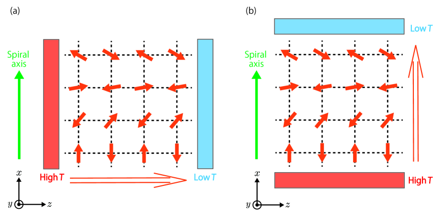
Figure 3: Schematic illustrations of the situations for (a) $\kappa_{zz}$ and (b) $\kappa_{xx}$. The red rectangles and blue rectangles represent the temperature gradient; the green arrows represent the spiral axis; the short and long arrows represent the spins and the magnon thermal currents, respectively.

We now turn to the inplane anisotropy of longitudinal thermal conductivities. For our screw-type spiral magnet on a $xz$ plane, the spiral axis is parallel to a $x$ axis and perpendicular to a $z$ axis, as shown in Fig. 1; this is because $\langle\bm{S}_{\bm{i}}\rangle={}^{t}(S\sin\bm{Q}\cdot\bm{i}\ 0\ S\cos\bm{Q}\cdot\bm{i})$ with $Q_{x}=\pi-\cos^{-1}(J/\sqrt{J^{2}+D^{2}})$ and $Q_{z}=\pi$. Since this spiral alignment in a $x$ direction results from the combination of the antiferromagnetic Heisenberg interaction and the Dzyaloshinsky-Moriya interaction, we expect that $\kappa_{xx}$ and $\kappa_{zz}$ are different and this difference is connected to a ratio of the Dzyaloshinsky-Moriya interaction to the Heisenberg interaction. To justify this expectation, we estimate $\kappa_{xx}/\kappa_{zz}$; the situations for $\kappa_{zz}$ and $\kappa_{xx}$ are schematically illustrated in Fig. 3. From Eqs. (66), (84), and (87) we have

$$\frac{\kappa_{xx}}{\kappa_{zz}}= \frac{\kappa_{xx}^{(\textrm{Born})}}{\kappa_{zz}^{(\textrm{Born})}}=\frac{\sum\limits_{\bm{q}}\tilde{e}^{x}(\bm{q})^{2}\Bigl{\{}-\frac{\partial n[\epsilon(\bm{q})]}{\partial\epsilon(\bm{q})}\Bigr{\}}\tilde{\tau}[\epsilon(\bm{q})]}{\sum\limits_{\bm{q}}\tilde{e}^{z}(\bm{q})^{2}\Bigl{\{}-\frac{\partial n(\epsilon_{\bm{q}})}{\partial\epsilon(\bm{q})}\Bigr{\}}\tilde{\tau}[\epsilon(\bm{q})]}.$$ (89)

Since the contributions for small $q=|\bm{q}|$ are dominant due to the $\{-\frac{\partial n[\epsilon(\bm{q})]}{\partial\epsilon(\bm{q})}\}$, we estimate $\kappa_{xx}/\kappa_{zz}$ by replacing $\bm{q}$ in $\tilde{e}^{x}(\bm{q})^{2}$ and $\tilde{e}^{z}(\bm{q})^{2}$ by $\bm{q}_{0}$; as described above, $\bm{q}_{0}$ is a certain momentum whose magnitude is small. As a result, $\kappa_{xx}/\kappa_{zz}$ is estimated as follows:

$$\frac{\kappa_{xx}}{\kappa_{zz}}\sim\frac{\tilde{e}^{x}(\bm{q}_{0})^{2}}{\tilde{e}^{z}(\bm{q}_{0})^{2}}=\frac{e_{11}^{x}(\bm{q}_{0})^{2}+e_{12}^{x}(\bm{q}_{0})^{2}\sinh^{2}2\theta_{\bm{q}_{0}}}{e_{11}^{z}(\bm{q}_{0})^{2}+e_{12}^{z}(\bm{q}_{0})^{2}\sinh^{2}2\theta_{\bm{q}_{0}}}.$$ (90)

To estimate this quantity, we calculate the numerator and denominator by considering the dominant terms including the leading correction from $D/J$ because $D$ will be typically smaller than $J$. After some calculations, described in Appendix H, we obtain

$$\frac{\kappa_{xx}}{\kappa_{zz}}\sim 1+\frac{3}{8}\Bigl{(}\frac{D}{J}\Bigr{)}^{2}q_{0}^{2}.$$ (91)

Thus the inplane anisotropy of longitudinal thermal conductivities is proportional to the squared ratio of the Dzyaloshinsky-Moriya interaction to the Heisenberg interaction:

$$\frac{\kappa_{xx}-\kappa_{zz}}{\kappa_{zz}}\propto\Bigl{(}\frac{D}{J}\Bigr{)}^{2}.$$ (92)

This result indicates that it is possible to estimate the magnitude of $D/J$ by measuring the inplane anisotropy of longitudinal thermal conductivities.

V Discussion

We first compare properties for the disordered spiral magnet and the disordered collinear antiferromagnet Lett . The same properties are global time-reversal symmetry, the diverging behavior of the particle-particle type four-point vertex function for the back scattering, and the negative logarithmic divergence of $\Delta\kappa_{\alpha\alpha}$ for $L\rightarrow\infty$. This suggests that the weak localization of magnons is not unique only for the disordered collinear antiferromagnet, but ubiquitous for the disordered magnets having global time-reversal symmetry. The major differences are the alignments of spins and the inplane anisotropy of longitudinal thermal conductivities: only one of the three components of $\langle\hat{S}^{\alpha}_{\bm{i}}\rangle$ ($\alpha=x,y,z$) is finite in the collinear antiferromagnet, whereas two are finite in the screw-type spiral magnet; $\kappa_{xx}$ and $\kappa_{yy}$ are the same in the collinear antiferromagnet on a $xy$ plane, whereas $\kappa_{xx}$ and $\kappa_{zz}$ are different in the screw-type spiral magnet on a $xz$ plane. The difference in the spin alignments arises from the effect of the Dzyaloshinsky-Moriya interaction, which is finite only for the screw-type spiral magnet. The difference in the inplane anisotropy of $\kappa_{\alpha\alpha}$ arises from the different spin alignments; in the screw-type spiral magnet the inplane longitudinal thermal conductivities become anisotropic due to the difference between magnon propagations parallel and perpendicular to the spiral axis.

We next discuss the validity of our approximation. We used the linear-spin-wave approximation, which took account of the quadratic terms of magnon operators. We believe this approximation is sufficient to analyze transport properties for low-energy magnons in two-dimensional magnets at low temperatures because several previous theoretical studies suggest that the terms neglected in the linear-spin-wave approximation may not change our main results at least qualitatively. First, some studies RMP-AF for a $S=1/2$ Heisenberg antiferromagnet on a square lattice show that the effects of the zero-point fluctuations and the magnon-magnon interaction are small at low temperatures. This result suggests that the corrections due to the zeroth-order term of magnon operators and the fourth-order (and higher-order) terms will be small at least at low temperatures. Then the theoretical studies for noncollinear antiferromagnets Shiba-chiral ; RMP-chiral show that the third-order terms of magnon operators induce the magnon-magnon interaction characteristic of noncollinear magnets, such as spiral magnets, and that its effects on the energy dispersion and damping for low-energy magnons are small. Since low-energy magnons give the dominant contributions to the longitudinal thermal conductivities of magnons, the third-order terms also may not change our main results at least qualitatively.

We turn to implications for further theoretical studies. First, an analogy with the disordered collinear antiferromagnet Full suggests that the disordered screw-type spiral magnet may show a characteristic property of magnetothermal magnon transport in the presence of a weak external magnetic field. This could be demonstrated by the theory for the disordered spiral magnet with the weak external magnetic field. Second, by combining our theory without using the two simplifications with first-principles calculations, it is possible to study material varieties of the weak localization of magnons in various disordered magnets. For the first-principles calculations, a set of Eqs. (66)–(73) is more appropriate than the theory using the two simplifications. Third, our theory can be extended to not only other disordered spiral magnets, but also disordered chiral magnets, which have finite spin scalar chirality. Whereas spin scalar chirality for certain three sites breaks local time-reversal symmetry for the three sites, global time-reversal symmetry could hold in some disordered chiral magnets; this could be possible if the disordered chiral magnet has the magnetic structure consisting of time-reversal symmetric pairs for spin scalar chirality [e.g., $\langle\hat{\bm{S}}_{\bm{i}}\cdot(\hat{\bm{S}}_{\bm{j}}\times\hat{\bm{S}}_{\bm{k}})\rangle$ and $\langle\hat{\bm{S}}_{\bm{i}^{\prime}}\cdot(\hat{\bm{S}}_{\bm{j}^{\prime}}\times\hat{\bm{S}}_{\bm{k}^{\prime}})\rangle=-\langle\hat{\bm{S}}_{\bm{i}}\cdot(\hat{\bm{S}}_{\bm{j}}\times\hat{\bm{S}}_{\bm{k}})\rangle$].

We finally discuss implications for experiments. First, the weak localization of magnons in our disordered spiral magnet can be experimentally observed by measuring $\kappa_{\alpha\alpha}$. If $\kappa_{\alpha\alpha}$ is measured at very low temperatures, at which the inelastic scattering due to the magnon-magnon interaction is negligible, the weak localization of magnons will be observed as the drastic suppression of the magnon thermal current parallel to temperature gradient as a result of the logarithmic dependence of $\Delta\kappa_{\alpha\alpha}$ on $L$. If the measurement is performed at low temperatures, at which the inelastic scattering is small but non-negligible, the weak localization of magnons would be observed as the logarithmic temperature dependence of $\kappa_{\alpha\alpha}$; this is based on a similar argument Lett to the effect of the inelastic scattering for electrons Thouless-Inela ; Anderson-Inela . Second, the inplane anisotropy of longitudinal thermal conductivities could be used to experimentally estimate the magnitude of $D/J$ in the screw-type spiral magnet. In particular, this method may be convenient for experimentally estimating whether the Dzyaloshinsky-Moriya interaction is small or large. Third, our main results, the weak localization of magnons and the inplane anisotropy of longitudinal thermal conductivities, may be realized in a real material, for example, Ba₂Cu_1-xAg_xGe₂O₇. The magnetic properties of Ba₂CuGe₂O₇ are described by the spin Hamiltonian consisting of the antiferromagnetic Heisenberg interaction and the Dzyaloshinsky-Moriya interaction for $S=1/2$ Cu²⁺ ions CuSpiral1 ; CuSpiral2 ; CuSpiral3 . Furthermore, Ba₂CuGe₂O₇ at very low temperatures can be regarded as a screw-type spiral magnet on a square lattice CuSpiral1 ; CuSpiral2 ; CuSpiral3 ; in this magnet, the spin alignment along a direction on the square lattice is spiral, and the spin alignment along the perpendicular direction is antiferromagnetic. These spin alignments are similar to those for our screw-type spiral magnet, whereas there are some differences in the details. Then replacing part of Cu ions by Ag ions will be suitable for impurities because this replacement keeps the spin quantum number $S$ unchanged and its main effect is to modify the exchange interactions Lett ; Full . We believe Ba₂Cu_1-xAg_xGe₂O₇ is a probable material for the weak localization of magnons and the inplane anisotropy of longitudinal thermal conductivities. This is because the inplane anisotropy results from the difference between magnon propagation along the spiral spin alignment and along the antiferromagnetic spin alignment, and because the magnetic structure of Ba₂Cu_1-xAg_xGe₂O₇ without external fields may have global time-reversal symmetry and such spin alignments.

VI Summary

We have studied the longitudinal thermal conductivities of magnons in the disordered screw-type spiral magnet in the weak-localization regime. We used the spin Hamiltonian consisting of the antiferromagnetic Heisenberg interaction and the Dzyaloshinsky-Moriya interaction on a square lattice on a $xz$ plane. We also considered the mean-field type spin Hamiltonian of impurities by treating disorder effects as the changes of these exchange interactions. By using the linear-response theory with the linear-spin-wave approximation for the screw-type spiral magnet and performing the perturbation calculations, we derived the longitudinal thermal conductivities including the main correction term in the weak-localization regime. We showed that $\kappa_{xx}$ and $\kappa_{zz}$ are different due to the difference between magnon propagations parallel and perpendicular to the spiral axis. This anisotropy is different from the isotropic result in the disordered two-dimensional antiferromagnet, and its measurement may be useful for experimentally estimating the magnitude of $D/J$. We also showed that the main correction term gives the negative logarithmic divergence in the thermodynamic limit due to the critical back scattering. This is the same as the weak localization of magnons in the disordered two-dimensional antiferromagnet Lett , and thus suggests the generality of the weak localization of magnons in the disordered two-dimensional magnets having global time-reversal symmetry.

Appendix A Remarks about coherence of the back scattering

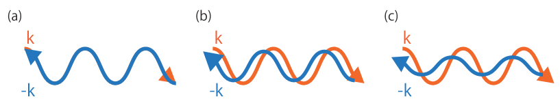
Figure 4: Schematic illustrations of the possible relations between the wave packets for $\bm{k}$ and $-\bm{k}$. Panel (a) shows the perfectly coherent case, whereas panels (b) and (c) show imperfectly coherent cases; in our definition the back scattering only in panel (a) is the coherent one. The amplitude difference and phase difference in panel (b) are smaller than in panel (c).

In this appendix we explain our definition of the coherent back scattering and its implications. We also show the relation between the coherence of the back scattering and the time-reversal symmetry of a system.

In our definition the back scattering is coherent only if the amplitude and the phase of the back scattered wave packet, the wave packet for $-\bm{k}$, are the same as those of the wave packet for $\bm{k}$ [Fig. 4(a)]. Even if the amplitude remains high and the phase difference is small [Fig. 4(b)], such back scattering is not the coherent one in our definition. Figure 4 shows the possible relations between the wave packets for $\bm{k}$ and $-\bm{k}$.

We have used this definition because only in the perfectly coherent case the wave packets for $\bm{k}$ and $-\bm{k}$ can form the standing wave even in the weak-localization regime. In an imperfectly coherent case the imbalance between the wave packets for $\bm{k}$ and $-\bm{k}$ could lead to finite conduction in the weak-localization regime. Actually, in such a case the back scattering amplitude is suppressed PhotoLoc compared with that in the perfectly coherent case. This suppression, as well as the suppression of the critical back scattering Full , results from the effect of the time-reversal symmetry breaking.

Then we can see the relation between coherence of the back scattering and time-reversal symmetry of a system from the following arguments. To see that relation, we argue the property of time reversal for a single-particle Green’s function. The retarded single-particle Green’s function is defined as $G^{(\textrm{R})}(\bm{k},\omega)\equiv\langle\bm{k}|\frac{1}{\omega-H+i\delta}|\bm{k}\rangle$, where $H$ is the Hamiltonian of a system. We assume that $H$ has time-reversal symmetry. This means $H\Theta=\Theta H$, where $\Theta$ is the time-reversal operator Sakurai . Since $\Theta$ is antiunitary, we have $\langle\beta|\alpha\rangle=\langle\alpha^{\prime}|\beta^{\prime}\rangle$, where $|\alpha^{\prime}\rangle=\Theta|\alpha\rangle$ and $|\beta^{\prime}\rangle=\Theta|\beta\rangle$. By applying this equation to the case for $|\alpha\rangle=\frac{1}{\omega-H+i\delta}|\bm{k}\rangle$ and $|\beta\rangle=|\bm{k}\rangle$ and using $H\Theta=\Theta H$, we obtain $G^{(\textrm{R})}(\bm{k},\omega)=G^{(\textrm{R})}(-\bm{k},\omega)$. This equation shows that as a result of time-reversal symmetry the single particles for $\bm{k}$ and $-\bm{k}$ have the same amplitude and phase.

Appendix B Ground-state properties of $\hat{H}_{0}$

In this appendix we show the ground-state properties of $\hat{H}_{0}$ in the mean-field approximation. For the details of the mean-field approximation for a spin Hamiltonian, see, for example, Refs. NA-Ir, , NA-pyro, , and Yosida-text, . In the mean-field approximation we can determine the most stable ground state for Eq. (2) by finding the lowest eigenvalue and the eigenfunction for the following equation under the hard-spin constraint:

$$\langle\hat{H}_{0}\rangle= \sum\limits_{\bm{i},\bm{j}}\sum\limits_{\alpha,\beta=x,y,z}M_{\alpha\beta}(\bm{i},\bm{j})\langle\hat{S}_{\bm{i}}^{\alpha}\rangle\langle\hat{S}_{\bm{j}}^{\beta}\rangle$$

$$= \sum\limits_{\bm{q}}\sum\limits_{\alpha,\beta=x,y,z}M_{\alpha\beta}(\bm{q})\langle\hat{S}_{\bm{q}}^{\alpha}\rangle^{\ast}\langle\hat{S}_{\bm{q}}^{\beta}\rangle$$

$$= \sum\limits_{\bm{q}}\langle\hat{\bm{S}}_{\bm{q}}\rangle^{\dagger}\left(\begin{array}[]{@{\,}ccc@{\,}}J(\bm{q})&0&D(\bm{q})^{\ast}\\ 0&J(\bm{q})&0\\ D(\bm{q})&0&J(\bm{q})\end{array}\right)\langle\hat{\bm{S}}_{\bm{q}}\rangle,$$ (96)

where

$$\langle\hat{S}_{\bm{i}}^{\alpha}\rangle=\frac{1}{\sqrt{N}}\sum\limits_{\bm{q}}e^{-i\bm{q}\cdot\bm{i}}\langle\hat{S}_{\bm{q}}^{\alpha}\rangle,$$ (97)

$$M_{\alpha\alpha}(\bm{q})=J(\bm{q})=J(\cos q_{x}+\cos q_{z}),$$ (98)

$$M_{zx}(\bm{q})=M_{xz}(\bm{q})^{\ast}=D(\bm{q})=iD\sin q_{x},$$ (99)

and $\langle\hat{S}_{\bm{i}}^{\alpha}\rangle$ satisfies the hard-spin constraint,

$$S^{2}=\frac{1}{N}\sum\limits_{\bm{i}}\sum\limits_{\alpha}|\langle\hat{S}_{\bm{i}}^{\alpha}\rangle|^{2}.$$ (100)

Since the eigenvalues of the $3\times 3$ matrix $M_{\alpha\beta}(\bm{q})$ are $\lambda_{0}(\bm{q})=J(\bm{q})$, $\lambda_{+}(\bm{q})=J(\bm{q})+|D(\bm{q})|$, and $\lambda_{-}(\bm{q})=J(\bm{q})-|D(\bm{q})|$, the minimum of $\lambda_{-}(\bm{q})$ is the lowest eigenvalue. For finite $J$ and $D$, $\lambda_{-}(\bm{q})$ is minimum at $\bm{q}=\bm{Q}={}^{t}(Q_{x}\ Q_{z})$, where $Q_{z}=\pi$, and $Q_{x}$ is determined by

$$\cos Q_{x}=-\frac{J}{\sqrt{J^{2}+D^{2}}},\ \sin Q_{x}=\frac{D}{\sqrt{J^{2}+D^{2}}}.$$ (101)

Since $\lambda_{-}(\bm{Q})=-J-\sqrt{J^{2}+D^{2}}$ is smaller than $\lambda_{-}(\bm{q})$ at $\bm{q}=\bm{Q}_{\textrm{AF}}={}^{t}(\pi\ \pi)$, $\lambda_{-}(\bm{Q}_{\textrm{AF}})=-2J$, the magnetic state for $\bm{q}=\bm{Q}$ is more stable than the antiferromagnetic state even for tiny $D$. Then we can determine the eigenfunction for the most stable ground state as follows. In the mean-field approximation for the magnetic state for $\bm{q}=\bm{Q}$ only $\langle\hat{\bm{S}}_{\bm{Q}}\rangle$ and $\langle\hat{\bm{S}}_{-\bm{Q}}\rangle$ are finite and the other $\langle\hat{\bm{S}}_{\bm{q}}\rangle$’s are zero. Since $\langle\hat{\bm{S}}_{\bm{Q}}\rangle$ is given by the eigenfunction for $M_{\alpha\beta}(\bm{Q})$, $\langle\hat{\bm{S}}_{\bm{Q}}\rangle=A{}^{t}(i\ 0\ 1)$, and $A$ is determined from Eq. (100), the magnetic structure for $\bm{q}=\bm{Q}$ is described by

$$\langle\bm{S}_{\bm{i}}\rangle=S\left(\begin{array}[]{@{\,}c@{\,}}\sin\bm{Q}\cdot\bm{i}\\ 0\\ \cos\bm{Q}\cdot\bm{i}\end{array}\right).$$ (105)

This equation with Eq. (101) and $Q_{z}=\pi$ show that the alignment of spins in a $x$ direction is spiral and the alignment in a $z$ direction is antiferromagnetic (see Fig. 1).

Appendix C Derivation of Eq. (20)

In this appendix we derive Eq. (20). By using Eqs. (17)–(19), we can express Eq. (2) as follows:

$$\hat{H}_{0}= \sum\limits_{\langle\bm{i},\bm{j}\rangle}\Bigl{\{}J_{\bm{i}\bm{j}}\cos[\bm{Q}\cdot(\bm{i}-\bm{j})]+D_{\bm{i}\bm{j}}\sin[\bm{Q}\cdot(\bm{i}-\bm{j})]\Bigr{\}}(\hat{S}_{\bm{i}}^{\prime x}\hat{S}_{\bm{j}}^{\prime x}+\hat{S}_{\bm{i}}^{\prime z}\hat{S}_{\bm{j}}^{\prime z})+\sum\limits_{\langle\bm{i},\bm{j}\rangle}J_{\bm{i}\bm{j}}\hat{S}_{\bm{i}}^{\prime y}\hat{S}_{\bm{j}}^{\prime y}$$

$$+\sum\limits_{\langle\bm{i},\bm{j}\rangle}\Bigl{\{}J_{\bm{i}\bm{j}}\sin[\bm{Q}\cdot(\bm{i}-\bm{j})]-D_{\bm{i}\bm{j}}\cos[\bm{Q}\cdot(\bm{i}-\bm{j})]\Bigr{\}}(\hat{S}_{\bm{i}}^{\prime z}\hat{S}_{\bm{j}}^{\prime x}-\hat{S}_{\bm{i}}^{\prime x}\hat{S}_{\bm{j}}^{\prime z}).$$ (106)

By using Eqs. (3), (4), and (101) and $Q_{z}=\pi$, the coefficients of the first and third terms in the above equation can be rewritten in a simpler expression: the coefficients for $\bm{j}-\bm{i}=(1\ 0)$ are

$$J_{\bm{i}\bm{j}}\cos[\bm{Q}\cdot(\bm{i}-\bm{j})]+D_{\bm{i}\bm{j}}\sin[\bm{Q}\cdot(\bm{i}-\bm{j})]=-\sqrt{J^{2}+D^{2}},$$ (107)

$$J_{\bm{i}\bm{j}}\sin[\bm{Q}\cdot(\bm{i}-\bm{j})]-D_{\bm{i}\bm{j}}\cos[\bm{Q}\cdot(\bm{i}-\bm{j})]=0,$$ (108)

and the coefficients for $\bm{j}-\bm{i}=(0\ 1)$ are

$$J_{\bm{i}\bm{j}}\cos[\bm{Q}\cdot(\bm{i}-\bm{j})]+D_{\bm{i}\bm{j}}\sin[\bm{Q}\cdot(\bm{i}-\bm{j})]=-J,$$ (109)

$$J_{\bm{i}\bm{j}}\sin[\bm{Q}\cdot(\bm{i}-\bm{j})]-D_{\bm{i}\bm{j}}\cos[\bm{Q}\cdot(\bm{i}-\bm{j})]=0.$$ (110)

Thus Eq. (106) is reduced to Eq. (20).

Appendix D Properties of the energy dispersion relation of magnon bands

In this appendix we explain several important properties of the energy dispersion relation of magnon bands for our spiral magnet. Before explaining the properties, we show the equation of $\epsilon(\bm{q})$ in terms of $J$ and $D$. Since $A(\bm{q})$ and $B(\bm{q})$ for our model are expressed as

$$A(\bm{q})=S(\sqrt{J^{2}+D^{2}}+J)-\frac{S}{2}(\sqrt{J^{2}+D^{2}}-J)\cos q_{x}$$ (111)

and

$$B(\bm{q})=-\frac{S}{2}(\sqrt{J^{2}+D^{2}}+J)\cos q_{x}-SJ\cos q_{z},$$ (112)

respectively, we obtain

$$\epsilon(\bm{q})= 2\sqrt{A(\bm{q})^{2}-B(\bm{q})^{2}}$$

$$= 2S\Bigl{[}2J^{2}+D^{2}+2J\sqrt{J^{2}+D^{2}}-D^{2}\cos q_{x}-(J^{2}+J\sqrt{J^{2}+D^{2}})\cos q_{x}\cos q_{z}$$

$$\ \ \ \ \ -J\sqrt{J^{2}+D^{2}}\cos^{2}q_{x}-J^{2}\cos^{2}q_{z}\Bigr{]}^{\frac{1}{2}}.$$ (113)

If we set $\bm{q}=\bm{0}$ in Eq. (113), we obtain $\epsilon(\bm{0})=0$. This means that the screw-type spiral magnet has the Goldstone-type gapless excitation. This is consistent with the argument based on the rotational symmetry in the spin space NA-JS because in our spiral magnet two of the three components of $\langle\hat{S}_{\bm{i}}^{\alpha}\rangle$ (i.e., $\langle\hat{S}_{\bm{i}}^{x}\rangle$ and $\langle\hat{S}_{\bm{i}}^{z}\rangle$) are finite and because in such a case the Goldstone-type gapless excitation is expected to exist without magnetic anisotropy terms.

Then, since the magnon energy is non-negative, the magnon energy is minimum at $\bm{q}=\bm{0}$ in our spiral magnet. This result is consistent with the assumption that the screw-type spiral state remains stable even including low-energy excitations, i.e., magnons, because magnons describe the displacement of spins from the ground-state alignment, because the magnon for $\bm{q}=\bm{0}$ corresponds to the uniform displacement, and because the uniform displacement induces no additional symmetry breaking. If the magnon energy is minimum at $\bm{q}=\bm{Q}_{\textrm{I}}$ and $-\bm{Q}_{\textrm{I}}$, this means either that magnons break a certain inversion symmetry which exists without magnons, or that it is necessary to choose a more stable ground state as the starting point for considering magnons.

Appendix E Derivation of Eq. (58)

In this appendix we derive Eq. (58) from Eq. (57) for $\hat{H}=\hat{H}_{0}$ for Eq. (25). This derivation consists of four steps. First, we decompose $\hat{h}_{\bm{i}}$ and $\hat{h}_{\bm{j}}$ in Eq. (57) as follows: $\hat{h}_{\bm{i}}=\hat{A}_{\bm{i}}+\hat{A}_{\bm{i}}^{\dagger}$ and $\hat{h}_{\bm{j}}=\hat{A}_{\bm{j}}+\hat{A}_{\bm{j}}^{\dagger}$, where

$$\hat{A}_{\bm{i}}=\frac{S}{4}\sum\limits_{\bm{l}}M_{\bm{i}\bm{l}}\hat{b}_{\bm{i}}^{\dagger}\hat{b}_{\bm{l}}-\frac{S}{4}\sum\limits_{\bm{l}}\tilde{J}^{(+)}_{\bm{i}\bm{l}}\hat{b}_{\bm{i}}\hat{b}_{\bm{l}},$$ (114)

with $M_{\bm{i}\bm{l}}=2\sum_{\bm{k}}\tilde{J}_{\bm{i}\bm{k}}\delta_{\bm{i},\bm{l}}-\tilde{J}_{\bm{i}\bm{l}}^{(-)}$. Because of these decompositions, Eq. (57) is reduced to

$$\hat{\bm{J}}_{E}= i\sum\limits_{\bm{m},\bm{n}}\bm{r}_{\bm{n}}[\hat{A}_{\bm{m}},\hat{A}_{\bm{n}}]+\Bigl{(}i\sum\limits_{\bm{m},\bm{n}}\bm{r}_{\bm{n}}[\hat{A}_{\bm{m}},\hat{A}_{\bm{n}}]\Bigr{)}^{\dagger}+i\sum\limits_{\bm{m},\bm{n}}\bm{r}_{\bm{n}}[\hat{A}_{\bm{m}},\hat{A}_{\bm{n}}^{\dagger}]+\Bigl{(}i\sum\limits_{\bm{m},\bm{n}}\bm{r}_{\bm{n}}[\hat{A}_{\bm{m}},\hat{A}_{\bm{n}}^{\dagger}]\Bigr{)}^{\dagger}.$$ (115)

Second, we calculate $[\hat{A}_{\bm{m}},\hat{A}_{\bm{n}}]$ and $[\hat{A}_{\bm{m}},\hat{A}_{\bm{n}}^{\dagger}]$. The results are as follows:

$$[\hat{A}_{\bm{m}},\hat{A}_{\bm{n}}] =\Bigl{(}\frac{S}{4}\Bigr{)}^{2}\sum\limits_{\bm{j},\bm{l}}M_{\bm{m}\bm{j}}M_{\bm{n}\bm{l}}(\hat{b}_{\bm{m}}^{\dagger}\hat{b}_{\bm{l}}\delta_{\bm{j},\bm{n}}-\hat{b}_{\bm{n}}^{\dagger}\hat{b}_{\bm{j}}\delta_{\bm{l},\bm{m}})+\Bigl{(}\frac{S}{4}\Bigr{)}^{2}\sum\limits_{\bm{j},\bm{l}}M_{\bm{m}\bm{j}}\tilde{J}^{(+)}_{\bm{n}\bm{l}}(\hat{b}_{\bm{n}}\hat{b}_{\bm{j}}\delta_{\bm{l},\bm{m}}+\hat{b}_{\bm{l}}\hat{b}_{\bm{j}}\delta_{\bm{n},\bm{m}})$$

$$-\Bigl{(}\frac{S}{4}\Bigr{)}^{2}\sum\limits_{\bm{j},\bm{l}}\tilde{J}^{(+)}_{\bm{m}\bm{j}}M_{\bm{n}\bm{l}}(\hat{b}_{\bm{m}}\hat{b}_{\bm{l}}\delta_{\bm{j},\bm{n}}+\hat{b}_{\bm{j}}\hat{b}_{\bm{l}}\delta_{\bm{n},\bm{m}}),$$ (116)

$$[\hat{A}_{\bm{m}},\hat{A}_{\bm{n}}^{\dagger}] =\Bigl{(}\frac{S}{4}\Bigr{)}^{2}\sum\limits_{\bm{j},\bm{l}}M_{\bm{m}\bm{j}}M_{\bm{n}\bm{l}}(\hat{b}_{\bm{m}}^{\dagger}\hat{b}_{\bm{n}}\delta_{\bm{j},\bm{l}}-\hat{b}_{\bm{l}}^{\dagger}\hat{b}_{\bm{j}}\delta_{\bm{n},\bm{m}})-\Bigl{(}\frac{S}{4}\Bigr{)}^{2}\sum\limits_{\bm{j},\bm{l}}M_{\bm{m}\bm{j}}\tilde{J}^{(+)}_{\bm{n}\bm{l}}(\hat{b}_{\bm{m}}^{\dagger}\hat{b}_{\bm{n}}^{\dagger}\delta_{\bm{l},\bm{j}}+\hat{b}_{\bm{m}}^{\dagger}\hat{b}_{\bm{l}}^{\dagger}\delta_{\bm{n},\bm{j}})$$

$$-\Bigl{(}\frac{S}{4}\Bigr{)}^{2}\sum\limits_{\bm{j},\bm{l}}\tilde{J}^{(+)}_{\bm{m}\bm{j}}M_{\bm{n}\bm{l}}(\hat{b}_{\bm{m}}\hat{b}_{\bm{n}}\delta_{\bm{j},\bm{l}}+\hat{b}_{\bm{j}}\hat{b}_{\bm{n}}\delta_{\bm{l},\bm{m}})$$

$$+\Bigl{(}\frac{S}{4}\Bigr{)}^{2}\sum\limits_{\bm{j},\bm{l}}\tilde{J}^{(+)}_{\bm{m}\bm{j}}\tilde{J}^{(+)}_{\bm{n}\bm{l}}(\hat{b}_{\bm{m}}\hat{b}_{\bm{n}}^{\dagger}\delta_{\bm{j},\bm{l}}+\hat{b}_{\bm{m}}\hat{b}_{\bm{l}}^{\dagger}\delta_{\bm{j},\bm{n}}+\hat{b}_{\bm{l}}^{\dagger}\hat{b}_{\bm{j}}\delta_{\bm{m},\bm{n}}+\hat{b}_{\bm{n}}^{\dagger}\hat{b}_{\bm{j}}\delta_{\bm{l},\bm{m}}).$$ (117)

Third, we combine these equations with Eq. (115). After some algebra, we obtain

$$\hat{\bm{J}}_{E}= 2i\Bigl{(}\frac{S}{4}\Bigr{)}^{2}\sum\limits_{\bm{m},\bm{n},\bm{l}}(-\bm{r}_{\bm{n}}+\bm{r}_{\bm{l}})M_{\bm{m}\bm{l}}M_{\bm{n}\bm{m}}\hat{b}_{\bm{n}}^{\dagger}\hat{b}_{\bm{l}}+2i\Bigl{(}\frac{S}{4}\Bigr{)}^{2}\sum\limits_{\bm{m},\bm{n},\bm{l}}(\bm{r}_{\bm{n}}-\bm{r}_{\bm{m}})\tilde{J}^{(+)}_{\bm{m}\bm{l}}\tilde{J}^{(+)}_{\bm{n}\bm{l}}\hat{b}_{\bm{m}}\hat{b}_{\bm{n}}^{\dagger}$$

$$+2i\Bigl{(}\frac{S}{4}\Bigr{)}^{2}\sum\limits_{\bm{m},\bm{n},\bm{l}}(\bm{r}_{\bm{n}}-\bm{r}_{\bm{l}})\tilde{J}^{(+)}_{\bm{n}\bm{m}}M_{\bm{m}\bm{l}}\hat{b}_{\bm{n}}\hat{b}_{\bm{l}}-2i\Bigl{(}\frac{S}{4}\Bigr{)}^{2}\sum\limits_{\bm{m},\bm{n},\bm{l}}(\bm{r}_{\bm{n}}-\bm{r}_{\bm{l}})M_{\bm{m}\bm{l}}\tilde{J}^{(+)}_{\bm{n}\bm{m}}\hat{b}_{\bm{l}}^{\dagger}\hat{b}_{\bm{n}}^{\dagger}.$$ (118)

Fourth, by using the Fourier coefficient of each quantity in Eq. (118), we express $\hat{\bm{J}}_{E}$ as a function of a momentum. By carrying out this calculation, we obtain Eq. (58).

Appendix F Derivation of Eq. (82)

In this appendix we derive Eq. (82) from Eq. (73) with Eqs. (79) and (80). We here describe this derivation only for $\epsilon>0$ because the expression for $\epsilon<0$ can be similarly derived. By substituting Eqs. (79) and (80) for $\epsilon>0$ into Eq. (73), we can express $\Pi_{abcd}(\bm{Q},\epsilon)$ for $\epsilon>0$ as follows:

$$\Pi_{abcd}(\bm{Q},\epsilon)=\sum\limits_{\bm{q}_{1}}\frac{U_{b\alpha}(\bm{q}_{1})U_{c\alpha}(\bm{q}_{1})U_{d\alpha}(\bm{Q}-\bm{q}_{1})U_{a\alpha}(\bm{Q}-\bm{q}_{1})}{[\epsilon-\epsilon(\bm{q}_{1})+i\tilde{\gamma}(\epsilon)][\epsilon-\epsilon(\bm{Q}-\bm{q}_{1})-i\tilde{\gamma}(\epsilon)]}.$$ (119)

Since for small $Q$, $U_{a\nu}(\bm{Q}-\bm{q}_{1})\sim U_{a\nu}(\bm{q}_{1})$ and $\epsilon(\bm{Q}-\bm{q}_{1})\sim\epsilon(\bm{q}_{1})-\frac{\partial\epsilon(\bm{q}_{1})}{\partial\bm{q}_{1}}\cdot\bm{Q}=\epsilon(\bm{q}_{1})-\bm{v}_{\bm{q}_{1}}\cdot\bm{Q}$, we can approximate Eq. (119) as follows:

$$\Pi_{abcd}(\bm{Q},\epsilon)\sim\sum\limits_{\bm{q}_{1}}\frac{U_{b\alpha}(\bm{q}_{1})U_{c\alpha}(\bm{q}_{1})U_{d\alpha}(\bm{q}_{1})U_{a\alpha}(\bm{q}_{1})}{[\epsilon-\epsilon(\bm{q}_{1})+i\tilde{\gamma}(\epsilon)][\epsilon-\epsilon(\bm{q}_{1})+\bm{v}_{\bm{q}_{1}}\cdot\bm{Q}-i\tilde{\gamma}(\epsilon)]}.$$ (120)

For a rough estimate of Eq. (120) we approximate momentum-dependent $U_{a\alpha}(\bm{q}_{1})$ and $\bm{v}_{\bm{q}_{1}}$ as the typical values at a certain, small momentum $\bm{q}_{0}$, $U_{a\alpha}(\bm{q}_{0})=u_{a\alpha}$ and $\bm{v}_{\bm{q}_{0}}$; this will be sufficient because the dominant contributions come from the small-$q_{1}$ contributions. As a result of this approximation, Eq. (120) is expressed as follows:

$$\Pi_{abcd}(\bm{Q},\epsilon)\sim\sum\limits_{\bm{q}_{1}}\frac{u_{b\alpha}u_{c\alpha}u_{d\alpha}u_{a\alpha}}{[\epsilon-\epsilon(\bm{q}_{1})+i\tilde{\gamma}(\epsilon)][\epsilon-\epsilon(\bm{q}_{1})+\bm{v}_{\bm{q}_{0}}\cdot\bm{Q}-i\tilde{\gamma}(\epsilon)]}.$$ (121)

Here we have replaced $(\cosh^{2}\theta_{\bm{q}_{1}}+\sinh^{2}\theta_{\bm{q}_{1}})^{2}$ in $\tilde{\gamma}(\epsilon)$ by $(\cosh^{2}\theta_{\bm{q}_{0}}+\sinh^{2}\theta_{\bm{q}_{0}})^{2}=(c_{0}^{2}+s_{0}^{2})^{2}$. Then, by replacing the summation over $\bm{q}_{1}$ by the corresponding integral and carrying out this integral, we obtain

$$\Pi_{abcd}(\bm{Q},\epsilon) \sim u_{b\alpha}u_{c\alpha}u_{d\alpha}u_{a\alpha}N\pi\rho(\epsilon)\tilde{\tau}(\epsilon)[1-\frac{1}{8}\bm{v}_{\bm{q}_{0}}^{2}Q^{2}\tilde{\tau}(\epsilon)^{2}]=\frac{u_{b\alpha}u_{c\alpha}u_{d\alpha}u_{a\alpha}}{\gamma_{\textrm{imp}}(c_{0}^{2}+s_{0}^{2})^{2}}[1-D_{\textrm{S}}(\epsilon)Q^{2}\tilde{\tau}(\epsilon)].$$ (122)

This is Eq. (82) for $\epsilon>0$. We can also obtain Eq. (82) for $\epsilon<0$ by using Eqs. (79) and (80) for $\epsilon<0$ and carrying out the similar calculation.

Appendix G Derivation of Eq. (83)

In this appendix we derive Eq. (83). This derivation consists of three steps. First, we rewrite the Bethe-Salpeter equation in the matrix form. By introducing $4\times 4$ matrices for $\Gamma_{abcd}(\bm{Q},\epsilon)$ and $\Pi_{abcd}(\bm{Q},\epsilon)$,

$$\Gamma=\left(\begin{array}[]{@{\,}cccc@{\,}}\Gamma_{1111}(\bm{Q},\epsilon)&\Gamma_{1112}(\bm{Q},\epsilon)&\Gamma_{1121}(\bm{Q},\epsilon)&\Gamma_{1122}(\bm{Q},\epsilon)\\ \Gamma_{1211}(\bm{Q},\epsilon)&\Gamma_{1212}(\bm{Q},\epsilon)&\Gamma_{1221}(\bm{Q},\epsilon)&\Gamma_{1222}(\bm{Q},\epsilon)\\ \Gamma_{2111}(\bm{Q},\epsilon)&\Gamma_{2112}(\bm{Q},\epsilon)&\Gamma_{2121}(\bm{Q},\epsilon)&\Gamma_{2122}(\bm{Q},\epsilon)\\ \Gamma_{2211}(\bm{Q},\epsilon)&\Gamma_{2212}(\bm{Q},\epsilon)&\Gamma_{2221}(\bm{Q},\epsilon)&\Gamma_{2222}(\bm{Q},\epsilon)\end{array}\right),$$ (127)

$$\Pi=\left(\begin{array}[]{@{\,}cccc@{\,}}\Pi_{1111}(\bm{Q},\epsilon)&\Pi_{1112}(\bm{Q},\epsilon)&\Pi_{1121}(\bm{Q},\epsilon)&\Pi_{1122}(\bm{Q},\epsilon)\\ \Pi_{1211}(\bm{Q},\epsilon)&\Pi_{1212}(\bm{Q},\epsilon)&\Pi_{1221}(\bm{Q},\epsilon)&\Pi_{1222}(\bm{Q},\epsilon)\\ \Pi_{2111}(\bm{Q},\epsilon)&\Pi_{2112}(\bm{Q},\epsilon)&\Pi_{2121}(\bm{Q},\epsilon)&\Pi_{2122}(\bm{Q},\epsilon)\\ \Pi_{2211}(\bm{Q},\epsilon)&\Pi_{2212}(\bm{Q},\epsilon)&\Pi_{2221}(\bm{Q},\epsilon)&\Pi_{2222}(\bm{Q},\epsilon)\end{array}\right),$$ (132)

we can express the Bethe-Salpeter equation Eq. (72) as follows:

$$\Gamma=\gamma_{\textrm{imp}}^{2}\Pi+\gamma_{\textrm{imp}}\Pi\Gamma.$$ (133)

Solving this matrix equation, we obtain the formal solution,

$$\Gamma=M^{-1}\gamma_{\textrm{imp}}^{2}\Pi,$$ (134)

where $M^{-1}$ is the inverse matrix of $M_{abcd}$, given by

$$M_{abcd}=\delta_{a,d}\delta_{b,c}-\gamma_{\textrm{imp}}\Pi_{abcd}(\bm{Q},\epsilon).$$ (135)

Second, we calculate $M^{-1}$. By using Eqs. (132) and (135), we can express the $4\times 4$ matrix $M$ as follows:

$$M=\left(\begin{array}[]{@{\,}cccc@{\,}}1-A&-C&-C&-F\\ -C&-F&1-F&-D\\ -C&1-F&-F&-D\\ -F&-D&-D&1-B\end{array}\right),$$ (140)

where

$$A =\gamma_{\textrm{imp}}\Pi_{1111}(\bm{Q},\epsilon),$$ (141)

$$B =\gamma_{\textrm{imp}}\Pi_{2222}(\bm{Q},\epsilon),$$ (142)

$$C =\gamma_{\textrm{imp}}\Pi_{1112}(\bm{Q},\epsilon)=\gamma_{\textrm{imp}}\Pi_{1121}(\bm{Q},\epsilon)=\gamma_{\textrm{imp}}\Pi_{1211}(\bm{Q},\epsilon)=\gamma_{\textrm{imp}}\Pi_{2111}(\bm{Q},\epsilon),$$ (143)

$$D =\gamma_{\textrm{imp}}\Pi_{2221}(\bm{Q},\epsilon)=\gamma_{\textrm{imp}}\Pi_{2212}(\bm{Q},\epsilon)=\gamma_{\textrm{imp}}\Pi_{2122}(\bm{Q},\epsilon)=\gamma_{\textrm{imp}}\Pi_{1222}(\bm{Q},\epsilon),$$ (144)

$$F =\gamma_{\textrm{imp}}\Pi_{1122}(\bm{Q},\epsilon)=\gamma_{\textrm{imp}}\Pi_{1212}(\bm{Q},\epsilon)=\gamma_{\textrm{imp}}\Pi_{2112}(\bm{Q},\epsilon)$$

$$=\gamma_{\textrm{imp}}\Pi_{1221}(\bm{Q},\epsilon)=\gamma_{\textrm{imp}}\Pi_{2121}(\bm{Q},\epsilon)=\gamma_{\textrm{imp}}\Pi_{2211}(\bm{Q},\epsilon).$$ (145)

To obtain $M^{-1}$, we need to calculate the cofactor matrix and determinant of $M$. After some algebra, we obtain

$$M^{-1}=\frac{1}{\textrm{det}M}\left(\begin{array}[]{@{\,}cccc@{\,}}-1+2F+B&-C&-C&-F\\ -C&-F&-1+A+B+F&-D\\ -C&-1+A+B+F&-F&-D\\ -F&-D&-D&-1+A+2F\end{array}\right),$$ (150)

where

$$\textrm{det}M= -1+A+B+2F=\begin{cases}-D_{\textrm{S}}(\epsilon)Q^{2}\tilde{\tau}(\epsilon)\ \ \ \ \ \ \ \ \ (\epsilon>0),\\ -D_{\textrm{S}}(-\epsilon)Q^{2}\tilde{\tau}(-\epsilon)\ \ \ \ (\epsilon<0).\end{cases}$$ (151)

In deriving Eq. (151) we have used Eqs. (141), (142), (145) and Eq. (82). Third, we combine Eqs. (150), (134) and (132). As a result, $\Gamma_{abcd}(\bm{Q},\epsilon)$ is given by

$$\Gamma_{abcd}(\bm{Q},\epsilon)= -\frac{\gamma_{\textrm{imp}}}{\textrm{det}M}\gamma_{\textrm{imp}}\Pi_{abcd}(\bm{Q},\epsilon)=\begin{cases}\dfrac{u_{b\alpha}u_{c\alpha}u_{d\alpha}u_{a\alpha}\gamma_{\textrm{imp}}}{D_{\textrm{S}}(\epsilon)Q^{2}\tilde{\tau}(\epsilon)}\ (\epsilon>0),\\[8.0pt] \dfrac{u_{b\beta}u_{c\beta}u_{d\beta}u_{a\beta}\gamma_{\textrm{imp}}}{D_{\textrm{S}}(-\epsilon)Q^{2}\tilde{\tau}(-\epsilon)}\ \ (\epsilon<0).\end{cases}$$ (152)

Appendix H Derivation of Eq.(91)

In this appendix we derive Eq. (91) from Eq. (90) by calculating the dominant terms including the leading correction from $D/J$. Since the quantities on the right-hand side of Eq. (90) can be expressed in terms of $A(\bm{q}_{0})$, $B(\bm{q}_{0})$, $\partial A(\bm{q}_{0})/\partial\bm{q}_{0}$, and $\partial B(\bm{q}_{0})/\partial\bm{q}_{0}$, we first calculate the dominant terms of $\partial A(\bm{q})/\partial\bm{q}$ and $\partial B(\bm{q})/\partial\bm{q}$. From Eqs. (111) and (112) we obtain

$$\frac{\partial A(\bm{q})}{\partial q_{x}}= \frac{S}{2}(\sqrt{J^{2}+D^{2}}-J)\sin q_{x}\sim\frac{S}{4}\frac{D^{2}}{J}\sin q_{x},$$ (153)

$$\frac{\partial A(\bm{q})}{\partial q_{z}}= \ 0,$$ (154)

$$\frac{\partial B(\bm{q})}{\partial q_{x}}= \frac{S}{2}(\sqrt{J^{2}+D^{2}}+J)\sin q_{x}\sim SJ\sin q_{x}+\frac{S}{4}\frac{D^{2}}{J}\sin q_{x},$$ (155)

$$\frac{\partial B(\bm{q})}{\partial q_{z}}= SJ\sin q_{z}.$$ (156)

Second, by using these equations, we estimate $e_{11}^{\alpha}(\bm{q})$ and $e_{12}^{\alpha}(\bm{q})$. The results are as follows:

$$e_{11}^{x}(\bm{q}) \sim 2SJ\sin q_{x}B(\bm{q})\Bigl{[}1-\Bigl{(}\frac{D}{2J}\Bigr{)}^{2}\frac{A(\bm{q})-B(\bm{q})}{B(\bm{q})}\Bigr{]},$$ (157)

$$e_{11}^{z}(\bm{q}) \sim 2SJ\sin q_{z}B(\bm{q}),$$ (158)

$$e_{12}^{x}(\bm{q}) \sim-2SJ\sin q_{x}A(\bm{q})\Bigl{[}1+\Bigl{(}\frac{D}{2J}\Bigr{)}^{2}\frac{A(\bm{q})+B(\bm{q})}{A(\bm{q})}\Bigr{]},$$ (159)

$$e_{12}^{z}(\bm{q}) \sim-2SJ\sin q_{z}A(\bm{q}).$$ (160)

Third, by using these equations and Eq. (41), we rewrite the numerator and denominator in Eq. (90). We thus obtain

$$\frac{e_{11}^{x}(\bm{q}_{0})^{2}+e_{12}^{x}(\bm{q}_{0})^{2}\sinh^{2}2\theta_{\bm{q}_{0}}}{e_{11}^{z}(\bm{q}_{0})^{2}+e_{12}^{z}(\bm{q}_{0})^{2}\sinh^{2}2\theta_{\bm{q}_{0}}}=1+\frac{1}{2}\Bigl{(}\frac{D}{J}\Bigr{)}^{2}\frac{2A(\bm{q}_{0})^{2}-B(\bm{q}_{0})^{2}+A(\bm{q}_{0})B(\bm{q}_{0})}{2A(\bm{q}_{0})^{2}-B(\bm{q}_{0})^{2}}.$$ (161)

Then the dominant terms of $A(\bm{q}_{0})$ and $B(\bm{q}_{0})$ are given by $A(\bm{q}_{0})\sim 2SJ$ and $B(\bm{q}_{0})\sim-2SJ(1-\frac{q_{0}^{2}}{4})$; here we have approximated $\cos q_{0x}$ and $\cos q_{0z}$ as $\cos q_{0x}\sim 1-\frac{q_{0x}^{2}}{2}$ and $\cos q_{0z}\sim 1-\frac{q_{0z}^{2}}{2}$ and considered only the leading terms. By substituting these equations of $A(\bm{q}_{0})$ and $B(\bm{q}_{0})$ into Eq. (161), we finally obtain Eq. (91).

References

- (1) N. Arakawa and J.-i. Ohe, Phys. Rev. B 97, 020407(R) (2018).
- (2) N. Arakawa and J.-i. Ohe, Phys. Rev. B 96, 214404 (2017).
- (3) L. I. Schiff, Quantum Mechanics (McGraw-Hilll, New York, 1968).
- (4) J. J. Sakurai, Modern Quantum Mechanics (The Benjamin/Cummings Publishing Company, California, 1985).
- (5) G. Bergman, Physics Report 107, 1-58 (1984).
- (6) Y. Nagaoka, T. Ando, and H. Takayama, Localization, Quantum Hall Effect, and Density Wave (Iwanami Shoten, Tokyo, 2000) pp. 3-90. (in Japanese); Y. Nagaoka, Prog. Theor. Phys. Supp. 84, 1 (1985).
- (7) A. Zheludev, G. Shirane, Y. Sasago, N. Koide, and K. Uchinokura, Phys. Rev. B 54, 15 163 (1996).
- (8) A. Zheludev, S. Maslov, G. Shirane, Y. Sasago, N. Koide, and K. Uchinokura, Phys. Rev. B 57, 2968 (1998).
- (9) A. Zheludev, S. Maslov, G. Shirane, Y. Sasago, N. Koide, and K. Uchinokura, Phys. Rev. B 59, 11 432 (1999).
- (10) I. Dzyaloshinsky, J. Phys. Chem. Solids 4, 241 (1958).
- (11) T. Moriya, Phys. Rev. 120, 91 (1960).
- (12) A. Yoshimori, J. Phys. Soc. Jpn. 14, 807 (1959).
- (13) N. Arakawa, Phys. Rev. B 94, 174416 (2016).
- (14) The time-reversal symmetry of the Dzyaloshinsky-Moriya interaction can been seen from the following argument. The Dzyaloshinsky-Moriya interaction is expressed as . First, is symmetric about time reversal because the time-reversal operator Sakurai satisfies , i.e., . The coefficient also holds time-reversal symmetry. This can be seen, for example, from Eq. (2.8) of Ref. DM-Moriya, by using the following three facts: the coefficient includes not only the imaginary unit but also the matrix element of the orbital angular momentum ; satisfies and ; there is no sign change in the other quantities of the coefficient under time-reversal operation.
- (15) M. Evers, C. A. Müller, and U. Nowak, Phys. Rev. B 97, 184423 (2018).
- (16) A. G. Del Maestro and M. J. P. Gingras, J.Phys.:Condens.Matter 16, 3339 (2004).
- (17) S. Toth and B. Lake, J. Phys.: Condens. Matter 27, 166002 (2015).
- (18) N. Arakawa, J. Phys. Soc. Jpn. 86, 094705 (2017).
- (19) The relation between the band degeneracy and the time-reversal symmetry can be shown by analyzing the relation between the first and the second terms of the first line in Eq. (46) under time reversal. By applying the time-reversal operator Sakurai to the first term, we obtain . Thus time-reversal symmetry relates the magnons for and in our spiral magnet.
- (20) G. D. Mahan, Many-Particle Physics (Plenum, New York, 2000).
- (21) A. A. Abrikosov, L. P. Gor’kov and I. E. Dzyaloshinski, Methods of Quantum Field Theory in Statistical Physics (Dover, New York, 1963).
- (22) G. M. liashberg, Zh. Eksp. Teor. Fiz. 41, 1241 (1961) [Sov. Phys. JETP 14, 886 (1962)].
- (23) N. Arakawa, Phys. Rev. B 94, 045107 (2016).
- (24) E. Manousakis, Rev. Mod. Phys. 63, 1 (1991).
- (25) T. Ohyama and H. Shiba, J. Phys. Soc. Jpn. 62, 3277 (1993).
- (26) M. E. Zhitomirsky and A. L. Chernyshev, Rev. Mod. Phys. 85, 219 (2013).
- (27) D. J. Thouless, Phys. Rev. Lett. 39, 1167 (1977).
- (28) P. W. Anderson, E. Abrahams, and T. V. Ramakrishnan Phys. Rev. Lett. 43, 718 (1979).
- (29) F. A. Erbacher, R. Lenke and G. Maret, Europhys. Lett. 21, 551 (1993).
- (30) K. Yosida, Magnetism (Iwanami Shoten, Tokyo, 1991) (in Japanese).
- (31) N. Arakawa, Phys. Rev. B 95, 235438 (2017).