A survey on the lace expansion for the nearest-neighbor models on the BCC lattice

Abstract

The aim of this survey is to explain, in a self-contained and relatively beginner-friendly manner, the lace expansion for the nearest-neighbor models of self-avoiding walk and percolation that converges in all dimensions above 6 and 9, respectively. To achieve this, we consider a $d$-dimensional version of the body-centered cubic (BCC) lattice, on which it is extremely easy to enumerate various random-walk quantities. Also, we choose a particular set of bootstrapping functions, by which a notoriously complicated part of the lace-expansion analysis becomes rather transparent.

1 Introduction

The lace expansion is one of the few mathematically rigorous methods to prove critical behavior for various statistical-mechanical models in high dimensions. It can show that the two-point function for the concerned model, up to the critical point, is bounded by the Green function for the underlying random walk in high dimensions. During the course of learning this method, it also provides good exercises in various mathematical skills from graph theory and algebraic identities to Fourier analysis and probability theory.

First, we explain background, some historical facts and the purposes of this survey.

1.1 Background

Corporation of infinitely many particles results in various intriguing and challenging problems. One of those is to understand phase transitions and critical behavior of statistical-mechanical models, such as percolation and the ferromagnetic Ising model. For percolation, for example, it exhibits a phase transition when the bond-occupation parameter $p$ crosses its critical value $p_{\mathrm{c}}$. If $p$ is far below $p_{\mathrm{c}}$, each cluster of occupied vertices is so small that we may use standard probabilistic techniques for i.i.d. random variables to predict what happens in the subcritical phase. If $p$ is far above $p_{\mathrm{c}}$, on the other hand, vacant vertices can only form tiny islands and most of the other vertices are connected to form a single gigantic cluster. However, when $p$ is close to $p_{\mathrm{c}}$, the cluster of connected vertices from the origin may be extremely large but porous in a nontrivial way, and therefore naive perturbation methods fail.

A similar phenomenon occurs for self-avoiding walk (SAW), a century-old statistical-mechanical model for linear polymers. Consider a locally finite, amenable and transitive graph as space. A standard example is the $d$-dimensional integer lattice $\mathbb{Z}^{d}$. The main observable to be investigated is the SAW two-point function, which is the following generating function with fugacity $p\geq 0$:

$$G_{p}(x)=\sum_{\omega:o\to x}p^{|\omega|}\prod_{j=1}^{|\omega|}D(\omega_{j}-\omega_{j-1})\prod_{0\leq s<t\leq|\omega|}(1-\lambda\delta_{\omega_{s},\omega_{t}}),$$ (1.1)

where the sum is over the nearest-neighbor paths $\omega$ on the concerned lattice from the origin $o$ to $x$, $|\omega|$ is the number of steps along $\omega$, and $D$ is the 1-step distribution of simple random walk (RW): $D(x)=(2d)^{-1}\delta_{|x|,1}$ on $\mathbb{Z}^{d}$. The parameter $\lambda\in[0,1]$ is the intensity of self-avoidance; the model with $\lambda=1$ is called strictly SAW, while the one with $\lambda\in(0,1)$ is called weakly SAW. The two-point function with $\lambda=0$ is equivalent to the RW Green function $S_{p}(x)\equiv\sum_{n=0}^{\infty}p^{n}D^{*n}(x)$, where $D^{*n}$ is the $n$-fold convolution of $D$. The critical point (= the radius of convergence) for RW is $p=1$. For SAW, because of subadditivity, there is a critical point $p_{\mathrm{c}}\geq 1$ such that the susceptibility $\chi_{p}\equiv\sum_{x}G_{p}(x)$ is finite if and only if $p<p_{\mathrm{c}}$ and diverges as $p\uparrow p_{\mathrm{c}}$ (see, e.g., [ms93]).

The way $\chi_{p}$ diverges is intriguing, as it shows power-law behavior as $(p_{\mathrm{c}}-p)^{-\gamma}$ with the critical exponent $\gamma$. It is considered to be universal in the sense that the value of $\gamma$ depends only on $d$ and is insensitive to $\lambda\in(0,1]$ and the detail lattice structure. For example, the value of $\gamma$ for strictly SAW on $\mathbb{Z}^{2}$ is believed to be $\frac{43}{32}$ and equal to that for weakly SAW on the 2-dimensional triangular lattice. This is not the case for the critical point $p_{\mathrm{c}}$, as its value may vary depending on $\lambda\in(0,1]$ and the detail lattice structure. Other statistical-mechanical models that exhibit divergence of the susceptibility are also characterized by the critical exponent $\gamma$, and many physicists as well as mathematicians have been trying hard to identify the value of $\gamma$ and classify the models into different universality classes since last century.

1.2 The mean-field theory

Because of the nonlocal self-avoidance constraint $\prod_{0\leq s<t\leq|\omega|}(1-\lambda\delta_{\omega_{s},\omega_{t}})$ in (1.1), SAW does not enjoy the Markovian property, which holds only when $\lambda=0$. If there is a way to average out the self-avoidance effect and absorb it into the fugacity $p$, then $G_{p}(x)$ may be approximated by the RW Green function $S_{\mu}(x)$ with a mean-field fugacity $\mu=\mu(\mathbb{Z}^{d},\lambda,p)$, and therefore $\chi_{p}$ may be approximated by $\sum_{x}S_{\mu}(x)=(1-\mu)^{-1}$. Presumably, $\mu(p_{\mathrm{c}})=1$. If $\mu$ is left-differentiable at $p_{\mathrm{c}}$, then this implies $\chi_{p}\asymp(p_{\mathrm{c}}-p)^{-1}$ (i.e., $\chi_{p}$ is bounded above and below by positive multiples of $(p_{\mathrm{c}}-p)^{-1}$) as $p\uparrow p_{\mathrm{c}}$. In this respect, the mean-field value for the critical exponent $\gamma$ is 1.

However, realizing the above idea is highly nontrivial. As a first step, one may want to use perturbation theory from the mean-field model (i.e., $\lambda=0$). The expansion of the self-avoidance constraint in powers of $\lambda>0$ yields

$$\prod_{0\leq s<t\leq|\omega|}(1-\lambda\delta_{\omega_{s},\omega_{t}})=\sum_{\Gamma\in\mathcal{G}[0,|\omega|]}(-\lambda)^{|\Gamma|}\prod_{\{s,t\}\in\Gamma}\delta_{\omega_{s},\omega_{t}},$$ (1.2)

where $\Gamma$, which is called a graph, is a set of pairs of indices on $[0,|\omega|]\equiv\{0,1,\dots,|\omega|\}$, $\mathcal{G}[0,|\omega|]$ is a set of such graphs, and $|\Gamma|$ is the cardinality of $\Gamma$. The trivial contribution from $\Gamma\equiv\varnothing$ is the unperturbed solution $S_{p}(x)$, which is already bad because its radius of convergence is 1, while $p_{\mathrm{c}}\geq 1$. The first correction term proportional to $\lambda$ is

$$-\lambda\sum_{\omega:o\to x}p^{|\omega|}\prod_{j=1}^{|\omega|}D(\omega_{j}-\omega_{j-1})\sum_{0\leq s<t\leq|\omega|}\delta_{\omega_{s},\omega_{t}}=-\lambda\big{(}S_{p}(o)-1\big{)}S_{p}^{*2}(x).$$ (1.3)

The higher-order correction terms are more involved, but the radius of convergence of each term is always $p=1$. What is worse, the alternating series of those terms is absolutely convergent only when $p$ is close to zero, because the sum over $\Gamma\in\mathcal{G}[0,|\omega|]$ is potentially huge as long as $\lambda>0$. As a result, this naive expansion cannot be applied near $p_{\mathrm{c}}$ in order to justify the mean-field behavior.

1.3 The infrared bound

Instead of deriving the exact solution for $\chi_{p}$, one may seek bounds on $\chi_{p}$ or its derivative. Indeed, it is not so difficult to show that [ms93]

$$\frac{\chi_{p}^{2}}{1+\lambda p_{\mathrm{c}}^{2}G_{p_{\mathrm{c}}}^{*2}(o)}\leq\frac{\mathrm{d}(p\chi_{p})}{\mathrm{d}p}\leq\chi_{p}^{2}.$$ (1.4)

The second inequality implies that $\chi_{p}$ is always bounded below by $(1-p/p_{\mathrm{c}})^{-1}$. Moreover, the first inequality implies that $\chi_{p}$ is also bounded above by a multiple of $(1-p/p_{\mathrm{c}})^{-1}$, hence $\gamma=1$, if

$$G_{p_{\mathrm{c}}}^{*2}(o)=\lim_{p\uparrow p_{\mathrm{c}}}\int_{\mathbb{T}^{d}}\hat{G}_{p}(k)^{2}\frac{\mathrm{d}^{d}k}{(2\pi)^{d}}<\infty,$$ (1.5)

where $\hat{G}_{p}(k)$ is the Fourier transform of the SAW two-point function and $\mathbb{T}^{d}\equiv[-\pi,\pi]^{d}$ is the $d$-dimensional torus of side length $2\pi$ in the Fourier space. It is a sufficient condition for the mean-field behavior for $\chi_{p}$ and is called the bubble condition, named after the shape of the diagram consisting of two line segments. Whether or not the bubble condition holds depends on the behavior of $\hat{G}_{p}(k)$ in the infrared regime (i.e., around $k=0$).

For percolation, there is a similar condition to the bubble condition under which $\gamma$ and other critical exponents take on their mean-field values. It is the cubic integrability of $\hat{G}_{p}(k)$ and is called the triangle condition [an84]. Again, whether or not the triangle condition holds depends on the infrared behavior of $\hat{G}_{p}(k)$.

Usually, there is no a priori bounds on $\hat{G}_{p}(k)$. However, for some spin models with a strong symmetry condition called reflection positivity (e.g., the ferromagnetic Ising model with symmetric nearest-neighbor couplings satisfies this condition), the two-point function enjoys the following infrared bound [fss76]: for any $d>2$, there is a constant $K<\infty$ such that

$$\|(1-\hat{D})\hat{G}_{p}\|_{\infty}\equiv\sup_{k\in\mathbb{T}^{d}}\big{(}1-\hat{D}(k)\big{)}|\hat{G}_{p}(k)|\leq K\qquad\text{uniformly in $p$ close to }p_{\mathrm{c}}.$$ (1.6)

If $D$ is a symmetric, non-degenerate and finite-range distribution with variance $\sigma^{2}$, then $1-\hat{D}(k)\sim\frac{\sigma^{2}}{2d}|k|^{2}$ as $|k|\to 0$. Suppose that the infrared bound holds for SAW and percolation. Then

$$G_{p_{\mathrm{c}}}^{*n}(o)\leq\int_{\mathbb{T}^{d}}\bigg{(}\frac{K}{1-\hat{D}(k)}\bigg{)}^{n}\frac{\mathrm{d}^{d}k}{(2\pi)^{d}}\asymp\int_{\mathbb{T}^{d}}\frac{\mathrm{d}^{d}k}{|k|^{2n}},$$ (1.7)

which implies that the bubble condition holds in all dimensions $d>4$ and the triangle condition holds in all dimensions $d>6$.

On the other hand, there is some evidence (from hyperscaling inequalities, numerical simulations, conformal field theory and so on) to suggest that the critical exponents (if they exist) cannot take on their mean-field values simultaneously if $d<4$ for SAW and $d<6$ for percolation. In this respect, the critical dimension $d_{\mathrm{c}}$ is said to be 4 for SAW and 6 for percolation.

To complete the mean-field picture in high dimensions, it thus remains to show that the infrared bound (1.6) holds for all dimensions $d>d_{\mathrm{c}}$. Here, the lace expansion comes into play.

1.4 The lace expansion

In 1985, Brydges and Spencer [bs85] came up to a fascinating idea. First, they looked at the naive expansion (1.2). Next, from each $\Gamma\in\mathcal{G}[0,|\omega|]$, they isolated a connected graph $\Gamma_{0}\subset\Gamma$ of the origin. Then, they extracted a minimally connected graph $\mathcal{L}\subset\Gamma_{0}$ called a lace, and resummed all the other edges in $\Gamma\setminus\mathcal{L}$ to partially restore the self-avoidance constraint. This is what we nowadays call the algebraic lace expansion, named after the shape of the aforesaid minimally connected graph. Since then, the algebraic lace expansion has been successfully applied to other models, such as oriented percolation [ny93], lattice trees and lattice animals [hs90l].

Later in 1990s, Hara and Slade (e.g., [hs92a]) came up to a more intuitively understandable way of deriving the lace expansion. To distinguish it from the algebraic lace expansion, we sometimes call it the inclusion-exclusion lace expansion. This opened up the possibility of applying the lace expansion to a wider class of models, including (unoriented) percolation [hs90p], the contact process [s01], the Ising model [s07] and the (one-component) $\varphi^{4}$ model [s15].

From now on, we simply call the latter the lace expansion. We will show its derivation for strictly SAW in Section 4.1 and for percolation in Section 5.1.

The result of the lace expansion is formally explained by the following recursion equation similar to that for the RW Green function: for any $p<p_{\mathrm{c}}$, there are functions $I_{p}$ and $J_{p}$ such that

$$G_{p}(x)=I_{p}(x)+(J_{p}*G_{p})(x).$$ (1.8)

If $I_{p}$ and $J_{p}$ satisfy certain regularity conditions, then it is natural to believe that the global behavior of $G_{p}$ is also similar to that of the RW Green function and therefore the infrared bound (1.6) holds.

However, since $I_{p}$ and $J_{p}$ are described by an alternating series of the lace-expansion coefficients $\{\pi_{p}^{\scriptscriptstyle(n)}\}_{n=0}^{N}$, each of which involves complicated local interaction ($n$ represents the degree of complexity), it is certainly not true that the aforesaid regularity conditions always hold. In fact, the regularity conditions require the critical bubble $(D^{*2}*G_{p_{\mathrm{c}}}^{*2})(o)$ for SAW and the critical triangle $(D^{*2}*G_{p_{\mathrm{c}}}^{*3})(o)$ for percolation to be small, not to be merely finite. This seemingly tautological statement (i.e., the critical bubble/triangle have to be small in order to prove them to be finite) is taken care of by the so-called bootstrapping argument, which will be explained later in this survey.

During the course of the bootstrapping argument, we often assume that the number of neighbors per vertex is sufficiently large. Since each vertex has $2d$ neighbors on $\mathbb{Z}^{d}$, it means that $d$ is assumed to be large. For SAW, Hara and Slade [hs92a, hs92b] succeeded in showing that $d\geq 5$ is large enough to prove mean-field results. For percolation, however, the situation is not as good as for SAW. The best results so far were obtained by Fitzner and van der Hofstad [fh15b], in which they proved mean-field results for $d\geq 11$ by using NoBLE, a perturbation method from non-backtracking random walk (= memory-2 SAW).

There is another way to increase the number of neighbors per vertex. Instead of taking $d$ large, we may enlarge the range $L$ of neighbors. One such example is the spread-out lattice $\bar{\mathbb{Z}}_{L}^{d}$, in which two distinct vertices $x,y\in\mathbb{Z}^{d}$ satisfying $\|x-y\|_{\infty}\leq L$ are defined to be neighbors, hence $(2L+1)^{d}-1$ neighbors per vertex. By taking $L$ sufficiently large, all the models for which the lace expansion was obtained are proven to exhibit mean-field behavior for all $d$ above the predicted upper-critical dimensions [hs90l, hs90p, ms93, ny93, s01, s07, s15].

1.5 The purposes of this survey

Since we believe in universality, the mean-field results on the spread-out lattice $\bar{\mathbb{Z}}_{L}^{d}$, as long as $L<\infty$, are believed to hold on $\mathbb{Z}^{d}$ as well. This is proven to be true for SAW, but not yet for percolation. We want to get rid of the artificial parameter $L$ and come up to a decent nearest-neighbor lattice, on which 7-dimensional percolation is proven to exhibit the mean-field behavior. In an ongoing project with Lung-Chi Chen and Markus Heydenreich [chhks??], we analyze the lace expansion for percolation on a $d$-dimensional version of the body-centered cubic (BCC) lattice, which has better features than the standard $\mathbb{Z}^{d}$, as explained in the next section. Thanks to those features, enumeration of RW quantities relevant to the lace-expansion analysis becomes extremely simple. Also, since those RW quantities are much smaller than the $\mathbb{Z}^{d}$-counterparts, it is easy to get closer to the predicted upper-critical dimension without introducing too much technical complexity. One of the purposes of this survey is to explain the current status of the BCC work and reveal the potential problems to overcome for completion of the mean-field picture in high dimensions.

Another purpose of this survey is to provide a relatively short, self-contained note on the lace expansion for the nearest-neighbor models. Currently, the best references on $\mathbb{Z}^{d}$ are [hs92a, hs92b] for SAW and [fh15a, fh15b] for percolation. However, they are not necessarily accessible to beginners, due to their length ($36+93$ pages for SAW and $79+92$ pages for percolation) and complexity. This is really unfortunate because, as mentioned earlier, the lace expansion can provide a good playground for, e.g., graduate students who may want to apply mathematical concepts and skills they learned to interesting and important problems. Considering this situation, we will keep the material as simple as possible, instead of making all-out efforts to go down to the predicted upper-critical dimensions. That will be the final goal of [chhks??].

2 The models and the main result

First, we provide precise definitions of the BCC lattice, self-avoiding walk and percolation. Then, we show the main result and explain its proof assuming key propositions.

2.1 The body-centered cubic (BCC) lattice

The $d$-dimensional BCC lattice $\mathbb{L}^{\!d}$ is a graph that contains the origin $o=(0,\dots,0)$ and is generated by the set of neighbors $\{x=(x_{1},\dots,x_{d}):\prod_{j=1}^{d}|x_{j}|=1\}$. It is equivalent to $\mathbb{Z}^{d}$ when $d=1$ and 2 (modulo rotation by $\pi/4$) but is more crowded in higher dimensions in the sense that the degree of each vertex is $2^{d}$ on $\mathbb{L}^{\!d}$, while it is $2d$ on $\mathbb{Z}^{d}$. We write $x\sim y$ if $x,y\in\mathbb{L}^{\!d}$ are neighbors, i.e., $\prod_{j=1}^{d}|x_{j}-y_{j}|=1$. It is a natural extension of the standard 3-dimensional BCC structure (see Figure 1).

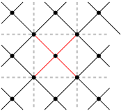
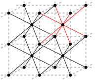
Figure 1: The basic structure (in red) of the BCC lattice $\mathbb{L}^{\!d}$ for $d=2,3$.

The $d$-dimensional Brownian motion with the identity covariance matrix can be constructed as the scaling limit of random walk (RW) on $\mathbb{L}^{\!d}$ generated by the 1-step distribution

$$D(x)=\frac{1}{2^{d}}\mathbbm{1}\raisebox{-1.0pt}{$\scriptstyle\{x\sim o\}$}=\prod_{j=1}^{d}\frac{1}{2}\delta_{|x_{j}|,1}.$$ (2.1)

Due to this factorization and Stirling’s formula, we can obtain a rather sharp bound on the $2n$-step return probability for all $n\in\mathbb{N}$, as

$$0\leq(\pi n)^{-d/2}-D^{*2n}(o)\leq\Big{(}1-e^{d(\frac{1}{24n+1}-\frac{1}{6n})}\Big{)}(\pi n)^{-d/2}\leq\frac{2d}{15n}(\pi n)^{-d/2}.$$ (2.2)

Using this, we can easily evaluate various RW quantities, such as the RW loop $\varepsilon_{1}$, the RW bubble $\varepsilon_{2}$ and the RW triangle $\varepsilon_{3}$, defined as

$$\varepsilon_{j} =(D^{*2}*S_{1}^{*j})(o)=\sum_{n=1}^{\infty}D^{*2n}(o)\times\begin{cases}1&[j=1],\\ (2n-1)&[j=2],\\ (2n-1)n&[j=3].\end{cases}$$ (2.3)

For example, if we split the sum into two at $n=N$, then the RW bubble $\varepsilon_{2}$ in dimensions $d>4$ can be estimated as

$$0\leq\varepsilon_{2}-\sum_{n=1}^{N}(2n-1)D^{*2n}(o)\leq 2\pi^{-d/2}\int_{N}^{\infty}t^{1-d/2}\,\mathrm{d}t=\frac{4\pi^{-d/2}}{d-4}N^{(4-d)/2}.$$ (2.4)

If we choose $d=5$ and $N=100$ and use a calculator to evaluate the sum over $n\leq N$, then we obtain $\varepsilon_{2}\leq 0.178465$. Table 1 summarizes the bounds on those RW quantities in different dimensions by choosing $N=500$ (so that, by (2.2), we can show that the RW triangle $\varepsilon_{3}$ for $d=7$ takes a value around the indicated number within $10^{-6}$).

Table 1: Upper bounds on the RW loop, bubble and triangle for $3\leq d\leq 9$.

	$d=3$	$d=4$	$d=5$	$d=6$	$d=7$	$d=8$	$d=9$
$\varepsilon_{1}$	0.393216	0.118637	0.046826	0.020461	0.009406	0.004451	0.002144
$\varepsilon_{2}$	$\infty$	$\infty$	0.178332	0.044004	0.015302	0.006156	0.002678
$\varepsilon_{3}$	$\infty$	$\infty$	$\infty$	$\infty$	0.052689	0.012354	0.004148

2.2 Self-avoiding walk

As declared at the end of Section 1, we restrict our attention to strictly SAW, which we simply call SAW from now on. Let $\Omega(x,y)$ be the set of self-avoiding paths on $\mathbb{L}^{\!d}$ from $x$ to $y$. By convention, $\Omega(x,x)$ is considered to be a singleton: a zero-step SAW at $x$. Then, the SAW two-point function defined in the previous section can be simplified as

$$G_{p}(x)=\sum_{\omega\in\Omega(o,x)}p^{|\omega|}\prod_{j=1}^{|\omega|}D(\omega_{j}-\omega_{j-1}),$$ (2.5)

where the empty product is regarded as 1. Recall that the susceptibility and its critical point are defined as

$$\chi_{p}=\sum_{x\in\mathbb{L}^{\!d}}G_{p}(x), p_{\mathrm{c}}=\sup\{p\geq 0:\chi_{p}<\infty\}.$$ (2.6)

For more background and related results before 1993, we refer to the “green” book by Madras and Slade [ms93]. For recent progress in various important problems, we refer to the monograph by Bauerschmidt et al. [bdcgs12].

2.3 Percolation

Here, we introduce bond percolation on $\mathbb{L}^{\!d}$. Each bond $\{u,v\}\subset\mathbb{L}^{\!d}$ randomly takes either one of the two states, occupied or vacant, independently of the other bonds. We define the bond-occupation probability of a bond $\{u,v\}$ as $pD(v-u)$, where $p\in[0,2^{d}]$ is the percolation parameter, which is equal to the expected number of occupied bonds per vertex. Let $\mathbb{P}_{p}$ be the associated probability measure, and denote its expectation by $\mathbb{E}_{p}$.

Next, we define the percolation two-point function. In order to do so, we first introduce the notion of connectivity. We say that a self-avoiding path $\omega=(\omega_{0},\dots,\omega_{|\omega|})\in\Omega(x,y)$ is occupied if either $x=y$ or every $b_{j}(\omega)\equiv\{\omega_{j-1},\omega_{j}\}$ for $j=1,\dots,|\omega|$ is occupied. We say that $x$ is connected to $y$, denoted by $x\longleftrightarrow y$, if there is an occupied self-avoiding path $\omega\in\Omega(x,y)$. Then, we define the percolation two-point function as

$$G_{p}(x)=\mathbb{P}_{p}(o\longleftrightarrow x) =\mathbb{P}_{p}\bigg{(}\bigcup_{\omega\in\Omega(o,x)}\{\omega\text{ is occupied}\}\bigg{)}.$$ (2.7)

The susceptibility $\chi_{p}$ and its critical point $p_{\mathrm{c}}$ are defined as in (2.6). Menshikov [m86] and Aizenman and Barsky [ab87] independently proved that $p_{\mathrm{c}}$ is unique in the sense that it can also be characterized by the emergence of an infinite cluster of the origin:

$$p_{\mathrm{c}}=\inf\big{\{}p\in[0,2^{d}]:\mathbb{P}_{p}(o\longleftrightarrow\infty)>0\big{\}}.$$ (2.8)

Recently, Duminil-Copin and Tassion [dct16] came up to a particularly simple proof of the uniqueness. They also extended the idea to the Ising model and dramatically simplified the proof of the uniqueness of the critical temperature, first proven by Aizenman, Barsky and Fernández [abf87].

For more background and related results before 1999, we refer to the excellent book by Grimmett [g99]. The book by Bollobás and Riordan [br06] also contains progress after publication of Grimmett’s book.

2.4 The main result

On the BCC lattice $\mathbb{L}^{\!d}$, we can prove the following result without introducing too much technical complexity.

Theorem 2.1 (Infrared bound).

For SAW on $\mathbb{L}^{\!d\geq 6}$ and percolation on $\mathbb{L}^{\!d\geq 9}$, there exists a model-dependent constant $K\in(0,\infty)$ such that

$$\|(1-\hat{D})\hat{G}_{p}\|_{\infty}\leq K\qquad\text{uniformly in }p\in[1,p_{\mathrm{c}}),$$ (2.9)

which implies the mean-field behavior, e.g., $\gamma=1$.

In the proof of a key proposition necessary for the above theorem, we will also show that $\chi_{1}<\infty$. This automatically implies the infrared bound for $p\in[0,1)$, since

$$\|(1-\hat{D})\hat{G}_{p}\|_{\infty}\leq 2\chi_{1}<\infty.$$ (2.10)

The above result for SAW is not as sharp as the result in [hs92a, hs92b], where Hara and Slade proved the infrared bound on $\mathbb{Z}^{d\geq 5}$. If we simply follow their analysis with the same amount of work, then we should be able to extend the above result to $\mathbb{L}^{\!d\geq 5}$. However, as is mentioned earlier, this is not our intention. We include the result for SAW as an example, just to show how easy to prove the infrared bound in such low dimensions with relatively small effort. Going down from 9 to 7 for percolation will require more serious effort. This will be the pursuit of the joint work [chhks??].

The proof of the above theorem is rather straightforward, assuming the following three propositions. To state those propositions, we first define

$$g_{1}(p)=p, g_{2}(p)=\|(1-\hat{D})\hat{G}_{p}\|_{\infty}.$$ (2.11)

Obviously, what we want to do is to show that $g_{2}(p)$ is bounded uniformly in $p\in[1,p_{\mathrm{c}})$. To define one more relevant function $g_{3}(p)$, we introduce the notation for a sort of second derivative in the Fourier space, in a particular direction. For a function $\hat{f}$ on $\mathbb{T}^{d}$ and $k,l\in\mathbb{T}^{d}$, we let

$$\hat{\Delta}_{k}\hat{f}(l)=\frac{\hat{f}(l+k)+\hat{f}(l-k)}{2}-\hat{f}(l).$$ (2.12)

By simple trigonometric calculation, it is shown in [s06, (5.17)] that the Fourier transform of the RW Green function $\hat{S}_{1}(k)\equiv(1-\hat{D}(k))^{-1}$, which is well-defined in a proper limit when $d>2$, obeys the inequality

$$|\hat{\Delta}_{k}\hat{S}_{1}(l)|$$

$$\leq\hat{U}(k,l)\equiv\big{(}1-\hat{D}(k)\big{)}\bigg{(}\frac{\hat{S}_{1}(l+k)+\hat{S}_{1}(l-k)}{2}\hat{S}_{1}(l)+4\hat{S}_{1}(l+k)\hat{S}_{1}(l-k)\bigg{)}.$$ (2.14)

Finally, we define

$$g_{3}(p)=\sup_{k,l}\frac{1}{\hat{U}(k,l)}\times\begin{cases}|\hat{\Delta}_{k}\hat{G}_{p}(l)|&[\mathrm{SAW}],\\ |\hat{\Delta}_{k}(\hat{G}_{p}(l)p\hat{D}(l))|&[\mathrm{percolation}],\end{cases}$$ (2.15)

where the supremum near $k=0$ should be interpreted as the supremum over the limit as $|k|\to 0$. It will be clear that $g_{3}$ is defined in slightly different ways between the two models, due to the difference in the recursion equations obtained by the lace expansion.

Now, we state the aforementioned three propositions and show that they indeed imply Theorem 2.1.

Proposition 2.2 (Continuity).

The functions $\{g_{i}(p)\}_{i=1}^{3}$ are continuous in $p\in[1,p_{\mathrm{c}})$.

Proposition 2.3 (Initial conditions).

For SAW on $\mathbb{L}^{\!d\geq 6}$ and percolation on $\mathbb{L}^{\!d\geq 8}$, there are model-dependent finite constants $\{K_{i}\}_{i=1}^{3}$ such that $g_{i}(1)<K_{i}$ for $i=1,2,3$.

Proposition 2.4 (Bootstrapping argument).

For SAW on $\mathbb{L}^{\!d\geq 6}$ and percolation on $\mathbb{L}^{\!d\geq 9}$, we fix $p\in(1,p_{\mathrm{c}})$ and assume $g_{i}(p)\leq K_{i}$, $i=1,2,3$, where $\{K_{i}\}_{i=1}^{3}$ are the same constants as in Proposition 2.3. Then, the stronger inequalities $g_{i}(p)<K_{i}$, $i=1,2,3$, hold.

Since $g_{2}(p)$ is continuous in $p\in[1,p_{\mathrm{c}})$, with the initial value $g_{2}(1)<K_{2}$, and cannot be equal to $K_{2}$ for $p\in(1,p_{\mathrm{c}}\wedge K_{1})$, we can say that the strict inequality $g_{2}(p)<K_{2}$ holds for all $p\in[1,p_{\mathrm{c}}\wedge K_{1})$. Since the same argument applies to $g_{1}(p)$, we can conclude $p_{\mathrm{c}}\leq K_{1}$, hence $g_{2}(p)<K_{2}$ for all $p\in[1,p_{\mathrm{c}})$ (see Figure 2). This completes the proof of Theorem 2.1 assuming Propositions 2.2–2.4.  

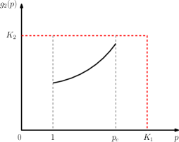
Figure 2: Depiction of the proof of Theorem 2.1 assuming Propositions 2.2–2.4.

2.5 Where and how to use the lace expansion

It remains to prove Propositions 2.2–2.4. The proof of Proposition 2.2 is elementary, though cumbersome for $g_{3}(p)$, and is explained in the next section. To prove the other two propositions, we will use the following lace expansion.

Proposition 2.5 (Lace expansion).

For any $p<p_{\mathrm{c}}$ and $N\in\mathbb{Z}_{+}\equiv\{0\}\cup\mathbb{N}$, there exist model-dependent nonnegative functions $\{\pi_{p}^{\scriptscriptstyle(n)}\}_{n=0}^{N}$ on $\mathbb{L}^{\!d}$ ($\pi_{p}^{\scriptscriptstyle(0)}\equiv 0$ for SAW) such that, if we define $I_{p}^{\scriptscriptstyle(N)}$ and $J_{p}^{\scriptscriptstyle(N)}$ as

$$I_{p}^{\scriptscriptstyle(N)}(x) =\delta_{o,x}+\begin{cases}0&[\text{SAW}],\\ \sum_{n=0}^{N}(-1)^{n}\pi_{p}^{\scriptscriptstyle(n)}(x)&[\text{percolation}],\end{cases}$$ (2.16)

$$J_{p}^{\scriptscriptstyle(N)}(x) =pD(x)+\begin{cases}\sum_{n=1}^{N}(-1)^{n}\pi_{p}^{\scriptscriptstyle(n)}(x)&[\text{SAW}],\\ \sum_{n=0}^{N}(-1)^{n}(\pi_{p}^{\scriptscriptstyle(n)}*pD)(x)&[\text{percolation}],\end{cases}$$ (2.17)

then we obtain the recursion equation

$$G_{p}(x)=I_{p}^{\scriptscriptstyle(N)}(x)+(J_{p}^{\scriptscriptstyle(N)}*G_{p})(x)+(-1)^{N+1}R_{p}^{\scriptscriptstyle(N+1)}(x),$$ (2.18)

where the remainder $R_{p}^{\scriptscriptstyle(N)}$ obeys the bound

$$0\leq R_{p}^{\scriptscriptstyle(N)}(x)\leq(\pi_{p}^{\scriptscriptstyle(N)}*G_{p})(x).$$ (2.19)

The derivation of the lace expansion is model-dependent and is explained for SAW in Section 4.1 and for percolation in Section 5.1.

Here, we briefly explain where and how to use the lace expansion to prove Propositions 2.3–2.4. The details will be given in later sections.

Step 1.  First, we evaluate $\{g_{i}(p)\}_{i=1}^{3}$ in terms of sums of $\hat{\pi}_{p}^{\scriptscriptstyle(n)}(k)\equiv\sum_{x}e^{ik\cdot x}\pi_{p}^{\scriptscriptstyle(n)}(x)$.

(i) Let $p\in[1,p_{\mathrm{c}})$ and suppose $\sum_{n=0}^{\infty}\hat{\pi}_{p}^{\scriptscriptstyle(n)}(0)$ is small enough to ensure that

$$\lim_{N\to\infty}\hat{\pi}_{p}^{\scriptscriptstyle(N)}(0)=0, \hat{I}_{p}(k)\equiv\lim_{N\to\infty}\hat{I}_{p}^{\scriptscriptstyle(N)}(k)>0~{}~{}\text{uniformly in }p\text{ and }k.$$ (2.20)

The latter is always true for SAW since $\hat{I}_{p}(k)\equiv 1$. The former implies that

$$0\leq\sum_{x\in\mathbb{L}^{\!d}}R_{p}^{\scriptscriptstyle(N)}(x)\leq\hat{\pi}_{p}^{\scriptscriptstyle(N)}(0)\chi_{p}\xrightarrow[N\to\infty]{}0.$$ (2.21)

Let (n.b. $\pi_{p}^{\scriptscriptstyle(0)}\equiv 0$ for SAW)

$$\hat{\Pi}_{p}(k)=\sum_{n=0}^{\infty}(-1)^{n}\hat{\pi}_{p}^{\scriptscriptstyle(n)}(k), \hat{J}_{p}(k)=p\hat{D}(k)+\begin{cases}\hat{\Pi}_{p}(k)&[\text{SAW}],\\ \hat{\Pi}_{p}(k)p\hat{D}(k)&[\text{percolation}].\end{cases}$$ (2.22)

Then, by using (2.18), we obtain

$$\chi_{p}\equiv\hat{G}_{p}(0)=\hat{I}_{p}(0)+\hat{J}_{p}(0)\chi_{p}=\frac{\hat{I}_{p}(0)}{1-\hat{J}_{p}(0)}.$$ (2.23)

Since $\chi_{p}\geq 0$ and $\hat{I}_{p}(0)>0$, we can conclude $\hat{J}_{p}(0)\leq 1$, which implies

$$g_{1}(p)\leq\begin{cases}1-\hat{\Pi}_{p}(0)&[\text{SAW}],\\ (1+\hat{\Pi}_{p}(0))^{-1}&[\text{percolation}].\end{cases}$$ (2.24)

(ii) Next, by (2.18) and (2.23), we obtain

$$\hat{G}_{p}(k)=\frac{\hat{I}_{p}(k)}{1-\hat{J}_{p}(k)}=\frac{\hat{I}_{p}(k)}{-\hat{\Delta}_{k}\hat{J}_{p}(0)+\hat{I}_{p}(0)/\chi_{p}},$$ (2.25)

where we have used the symmetry $\hat{J}_{p}(k)=\hat{J}_{p}(-k)$ to obtain $-\hat{\Delta}_{k}\hat{J}_{p}(0)=\hat{J}_{p}(0)-\hat{J}_{p}(k)$. Suppose $-\sum_{n=0}^{\infty}\hat{\Delta}_{k}\hat{\pi}_{p}^{\scriptscriptstyle(n)}(0)\equiv\sum_{n=0}^{\infty}\sum_{x}(1-\cos k\cdot x)\pi_{p}^{\scriptscriptstyle(n)}(x)$ is smaller than $1-\hat{D}(k)$ in order to ensure $-\hat{\Delta}_{k}\hat{J}_{p}(0)\geq 0$. Then, $\hat{G}_{p}(k)$ is bounded as

$$0\leq\hat{G}_{p}(k)\leq\frac{\hat{I}_{p}(k)}{-\hat{\Delta}_{k}\hat{J}_{p}(0)}.$$ (2.28)

Since $p\geq 1$, this implies

$$g_{2}(p)\leq\begin{cases}\displaystyle\sup_{k}\bigg{(}1+\frac{-\hat{\Delta}_{k}\hat{\Pi}_{p}(0)}{1-\hat{D}(k)}\bigg{)}^{-1}&[\text{SAW}],\\ \displaystyle\sup_{k}\bigg{(}1+\frac{1}{\hat{I}_{p}(k)}\frac{-\hat{\Delta}_{k}\hat{\Pi}_{p}(0)}{1-\hat{D}(k)}\bigg{)}^{-1}&[\text{percolation}],\end{cases}$$ (2.29)

where the supremum near $k=0$ should be interpreted as the supremum over the limit as $|k|\to 0$.

(iii) To evaluate $g_{3}(p)$, we want to use the identity (3). To do so for percolation, we first notice that, by using $\hat{I}_{p}(k)p\hat{D}(k)=\hat{J}_{p}(k)$ and (2.25), we obtain

$$\hat{G}_{p}(k)p\hat{D}(k)=\frac{\hat{J}_{p}(k)}{1-\hat{J}_{p}(k)}=\frac{1}{1-\hat{J}_{p}(k)}-1\equiv\hat{A}_{p}(k)-1,$$ (2.30)

hence $\hat{\Delta}_{k}(\hat{G}_{p}(l)p\hat{D}(l))=\hat{\Delta}_{k}\hat{A}_{p}(l)$. As a result, $g_{3}(p)$ for both models can be written as

$$g_{3}(p)=\sup_{k,l}\frac{|\hat{\Delta}_{k}\hat{A}_{p}(l)|}{\hat{U}(k,l)}.$$ (2.31)

Then, by using (3) with $a(x)=J_{p}(x)$, noting $\hat{A}_{p}(k)=(-\hat{\Delta}_{k}\hat{J}_{p}(0)+\hat{I}_{p}(0)/\chi_{p})^{-1}\geq 0$ and applying the Schwarz inequality as in [s06, Lemma 5.7], we obtain

$$g_{3}(p)\leq\sup_{k,l}\frac{1-\hat{D}(k)}{\hat{U}(k,l)}\bigg{(} \frac{\hat{A}_{p}(l+k)+\hat{A}_{p}(l-k)}{2}\hat{A}_{p}(l)\frac{|\hat{\Delta}_{k}\hat{J}_{p}(l)|}{1-\hat{D}(k)}$$

$$+4\hat{A}_{p}(l+k)\hat{A}_{p}(l-k)\frac{-\hat{\Delta}_{l}\widehat{|J_{p}|}(0)}{1-\hat{J}_{p}(l)}\,\frac{-\hat{\Delta}_{k}\widehat{|J_{p}|}(0)}{1-\hat{D}(k)}\bigg{)},$$ (2.32)

where

$$\widehat{|J_{p}|}(k)=\sum_{x\in\mathbb{L}^{\!d}}e^{ik\cdot x}|J_{p}(x)|.$$ (2.33)

We can further bound $|\hat{\Delta}_{k}\hat{J}_{p}(l)|$ and $-\hat{\Delta}_{k}\widehat{|J_{p}|}(0)\equiv\widehat{|J_{p}|}(0)-\widehat{|J_{p}|}(k)\geq 0$ in terms of sums of $|\hat{\Delta}_{k}\hat{\pi}_{p}^{\scriptscriptstyle(n)}(0)|$. However, to simplify the exposition, we refrain from doing so for now and postpone it to later sections.

So far, we have assumed that $\sum_{n=0}^{\infty}\hat{\pi}_{p}^{\scriptscriptstyle(n)}(0)$ and $-\sum_{n=0}^{\infty}\hat{\Delta}_{k}\hat{\pi}_{p}^{\scriptscriptstyle(n)}(0)$ are small enough to carry out the above computations. Sufficient conditions to this assumption are

$$\sum_{n=1}^{\infty}\hat{\pi}_{p}^{\scriptscriptstyle(n)}(0)<\infty, \sup_{k}\sum_{n=1}^{\infty}\frac{-\hat{\Delta}_{k}\hat{\pi}_{p}^{\scriptscriptstyle(n)}(0)}{1-\hat{D}(k)}<1$$ (2.34)

for SAW, and

$$\sum_{n=0}^{\infty}\hat{\pi}_{p}^{\scriptscriptstyle(n)}(0)+\sup_{k}\sum_{n=0}^{\infty}\frac{-\hat{\Delta}_{k}\hat{\pi}_{p}^{\scriptscriptstyle(n)}(0)}{1-\hat{D}(k)}<1$$ (2.35)

for percolation (cf., (LABEL:eq:g2bd-prebyBWr)). These conditions are to be verified eventually.  

Step 2.  As shown in (2.24), (2.29) and (2.5), the bootstrapping functions $\{g_{i}(p)\}_{i=1}^{3}$ are bounded in terms of sums of $\hat{\pi}_{p}^{\scriptscriptstyle(n)}(0)$ and sums of $|\hat{\Delta}_{k}\hat{\pi}_{p}^{\scriptscriptstyle(n)}(0)|$. In the second step, we evaluate those lace-expansion coefficients in terms of smaller diagrams, such as

$$L_{p}=\|(pD)^{*2}*G_{p}\|_{\infty}, B_{p}=\|(pD)^{*2}*G_{p}^{*2}\|_{\infty}, T_{p}=\|(pD)^{*2}*G_{p}^{*3}\|_{\infty}.$$ (2.36)

For example, we can bound $\hat{\pi}_{p}^{\scriptscriptstyle(n)}$ for $n\geq 2$ as

$$0\leq\hat{\pi}_{p}^{\scriptscriptstyle(n)}(0)\leq\begin{cases}B_{p}(p\|D\|_{\infty}+L_{p})r^{n-2}&[\text{SAW}],\\ (1+\frac{1}{2}B_{p}+T_{p})^{2}r\rho^{n-1}&[\text{percolation}],\end{cases}$$ (2.37)

where

$$r=p\|D\|_{\infty}+L_{p}+B_{p}, \rho=\bigg{(}1+\frac{1}{2}B_{p}+T_{p}\bigg{)}(r+T_{p})+T_{p}(2r+T_{p})$$ (2.38)

See Sections 4–5 for the proof of the above inequality and the bounds on $\hat{\pi}_{p}^{\scriptscriptstyle(0)}(0)$ and $\hat{\pi}_{p}^{\scriptscriptstyle(1)}(0)$. It will also be shown that the amplitude of $|\hat{\Delta}_{k}\hat{\pi}_{p}^{\scriptscriptstyle(n)}(0)|/(1-\hat{D}(k))$ is bounded in a similar fashion, with the common ratio $r$ for SAW and $\rho$ for percolation. Therefore, the assumptions made in Step 1 hold if $L_{p},B_{p},T_{p}$ and other diagrams in the bounds are small enough.  

Step 3.  In the final step, we investigate the aforesaid diagrams and prove that, by choosing appropriate values for $\{K_{i}\}_{i=1}^{3}$, those diagrams are indeed small enough for SAW on $\mathbb{L}^{\!d\geq 6}$ and for percolation on $\mathbb{L}^{\!d\geq 9}$.

(i) For $p=1$, we only need to use the trivial inequality $G_{1}(x)\leq S_{1}(x)$, $x\in\mathbb{L}^{\!d}$, for both models to obtain that, for $d>2$ (as mentioned earlier, $\hat{S}_{1}(k)\equiv(1-\hat{D}(k))^{-1}$ is well-defined in a proper limit when $d>2$),

$$L_{1}\leq\|D^{*2}*S_{1}\|_{\infty}=\int_{\mathbb{T}^{d}}\frac{\hat{D}(k)^{2}}{1-\hat{D}(k)}\,\frac{\text{d}^{d}k}{(2\pi)^{d}}=(D^{*2}*S_{1})(o)\equiv\varepsilon_{1}.$$ (2.39)

Similarly, we obtain

$$B_{1}\leq\varepsilon_{2}, T_{1}\leq\varepsilon_{3}.$$ (2.40)

Consulting with Table 1 in Section 2.1, we can see that, even in $d_{\mathrm{c}}+1$ dimensions, $r$ and $\rho$ in (2.38) are small enough for the bootstrapping functions $\{g_{i}(p)\}_{i=1}^{3}$ to be convergent.

(ii) The strategy for $p\in(1,p_{\mathrm{c}})$ is different from that for $p=1$, because there is no a priori bound on $G_{p}$ in terms of $S_{1}$. Here, we use the assumptions $g_{i}(p)\leq K_{i}$, $i=1,2,3$, to evaluate the diagrams. For example,

$$L_{p}\leq p^{2}\int_{\mathbb{T}^{d}}\hat{D}(k)^{2}|\hat{G}_{p}(k)|\,\frac{\text{d}^{d}k}{(2\pi)^{d}}\leq K_{1}^{2}K_{2}\underbrace{\int_{\mathbb{T}^{d}}\frac{\hat{D}(k)^{2}}{1-\hat{D}(k)}\,\frac{\text{d}^{d}k}{(2\pi)^{d}}}_{=\varepsilon_{1}}.$$ (2.41)

Similarly,

$$B_{p}\leq K_{1}^{2}K_{2}^{2}\varepsilon_{2}, T_{p}\leq K_{1}^{2}K_{2}^{3}\varepsilon_{3}.$$ (2.42)

As a result, $r$ and $\rho$ in (2.38) become functions of $\{K_{i}\}_{i=1,2}$. If we choose their values appropriately, then we can derive the improved bound $g_{1}(p)<K_{1}$ for all $d\geq d_{\mathrm{c}}+1$. To improve the bounds on $\{g_{i}(p)\}_{i=2,3}$, we also have to control $K_{3}$. This is the worst enemy that keeps us from going down to $d_{\mathrm{c}}+1$ dimensions. In [chhks??], we will make all-out efforts to overcome this problem.  

2.6 Organization

In the rest of this survey, we prove the above propositions in detail. In Section 3, we prove Proposition 2.2 for both models.

In Section 4, we prove Propositions 2.3–2.5 for SAW as follows. In Section 4.1, we explain the derivation of the lace expansion (Proposition 2.5) for SAW. In Section 4.2, we prove bounds on the lace-expansion coefficients in terms of basic diagrams, as briefly explained in Step 2 in Section 2.5. In Section 4.4, we prove bounds on those basic diagrams in terms of RW quantities, as explained in Step 3 in Section 2.5. Applying them to the bounds on the bootstrapping functions $\{g_{i}(p)\}_{i=1}^{3}$ obtained in Step 1 in Section 2.5, we prove Propositions 2.3–2.4 on $\mathbb{L}^{\!d\geq 6}$. Finally, in Section 4.5, we provide further discussion to potentially improve our results.

In Section 5, we prove Propositions 2.3–2.5 for percolation as follows. In Section 5.1, we derive the lace expansion (Proposition 2.5) for percolation. In Section 5.2, we prove bounds on the lace-expansion coefficients in terms of basic diagrams, as briefly explained in Step 2 in Section 2.5. In Section LABEL:ss:TVOHbd, we prove bounds on those basic diagrams in terms of RW quantities, as explained in Step 3 in Section 2.5. Applying them to the bounds on the bootstrapping functions $\{g_{i}(p)\}_{i=1}^{3}$ obtained in Step 1 in Section 2.5, we prove Proposition 2.3 on $\mathbb{L}^{\!d\geq 8}$ and Proposition 2.4 on $\mathbb{L}^{\!d\geq 9}$. In Section LABEL:ss:discussion-perc, we provide further discussion to potentially improve our results.

3 Continuity of the bootstrapping functions

In this section, we prove Proposition 2.2. First, we recall (2.11) and (2.15) for the bootstrapping functions $\{g_{i}(p)\}_{i=1}^{3}$. Obviously, $g_{1}(p)\equiv p$ is continuous. To prove continuity of the other two, we introduce

$$\tilde{g}_{2,k}(p) =\big{(}1-\hat{D}(k)\big{)}\hat{G}_{p}(k),$$ (3.1)

$$\tilde{g}_{3,k,l}(p) =\frac{1}{\hat{U}(k,l)}\times\begin{cases}\hat{\Delta}_{k}\hat{G}_{p}(l)&[\text{SAW}],\\ \hat{\Delta}_{k}(\hat{G}_{p}(l)\hat{D}(l))&[\text{percolation}],\end{cases}$$ (3.2)

and show that they are continuous in $p\in[1,p_{\mathrm{c}})$ for every $k,l\in\mathbb{T}^{d}$. However, since

$$g_{2}(p)=\sup_{k\in\mathbb{T}^{d}}|\tilde{g}_{2,k}(p)|, g_{3}(p)=\sup_{k,l\in\mathbb{T}^{d}}|\tilde{g}_{3,k,l}(p)|,$$ (3.3)

and the supremum of continuous functions is not necessarily continuous, we must be a bit more cautious here. The following elementary lemma provides a sufficient condition for the supremum to be continuous.

Lemma 3.1 (Lemma 5.13 of [s06], in our language).

Fix $p_{0}\in[1,p_{\mathrm{c}})$ and let $\{\hat{f}_{k}(p)\}_{k\in\mathbb{T}^{d}}$ be an equicontinuous family of functions in $p\in[1,p_{0}]$. Suppose that $\sup_{k\in\mathbb{T}^{d}}\hat{f}_{k}(p)<\infty$ for every $p\in[1,p_{0}]$. Then, $\sup_{k\in\mathbb{T}^{d}}\hat{f}_{k}(p)<\infty$ is continuous in $p\in[1,p_{0}]$.

Therefore, in order to prove continuity of $\{g_{i}(p)\}_{i=2,3}$ in $p\in[1,p_{\mathrm{c}})$, we want to show that $\{\tilde{g}_{2,k}(p)\}_{k\in\mathbb{T}^{d}}$ and $\{\tilde{g}_{3,k,l}(p)\}_{k,l\in\mathbb{T}^{d}}$ are equicontinuous families of functions in $p\in[1,p_{0}]$ for each $p_{0}\in[1,p_{\mathrm{c}})$. To prove this, it then suffices to show that the following (i) and (ii) hold.

1. $\tilde{g}_{2,k}(p)$ and $\partial_{p}\tilde{g}_{2,k}(p)$ are finite uniformly in $k\in\mathbb{T}^{d}$ and $p\in[1,p_{0}]$.

2. $\tilde{g}_{3,k,l}(p)$ and $\partial_{p}\tilde{g}_{3,k,l}(p)$ are finite uniformly in $k,l\in\mathbb{T}^{d}$ and $p\in[1,p_{0}]$.

To prove (i) is not so hard. By $0\leq 1-\hat{D}(k)\leq 2$, $|\hat{G}_{p}(k)|\leq\chi_{p}$ and the monotonicity of $\chi_{p}$ in $p$, we obtain $|\tilde{g}_{2,k}(p)|\leq 2\chi_{p_{0}}<\infty$ uniformly in $k\in\mathbb{T}^{d}$ and $p\in[1,p_{0}]$. Moreover, by subadditivity for SAW, Russo’s formula and the BK inequality for percolation (see, e.g., [g99]), and then using translation-invariance, we obtain

$$0\leq\partial_{p}G_{p}(x)\leq(D*G_{p}^{*2})(x),$$ (3.4)

hence

$$|\partial_{p}\tilde{g}_{2,k}(p)|\leq 2\sum_{x}(D*G_{p}^{*2})(x)\leq 2\chi_{p_{0}}^{2}<\infty,$$ (3.5)

uniformly in $k\in\mathbb{T}^{d}$ and $p\in[1,p_{0}]$, as required.

To prove (ii) needs extra care, especially near $k=0$, because of the factor $1-\hat{D}(k)$ in $\hat{U}(k,l)$. From here, we prove (ii) for SAW and for percolation separately.

Proof of (ii) for SAW.  First, by using the telescopic inequality in [fh15a, Appendix A]

$$0\leq 1-\cos\sum_{j=1}^{J}t_{j}\leq J\sum_{j=1}^{J}(1-\cos t_{j}),$$ (3.7)

we obtain

$$|\hat{\Delta}_{k}\hat{G}_{p}(l)|\leq\sum_{x}(1-\cos k\cdot x)G_{p}(x)$$

$$\quad=\sum_{x}\sum_{\omega\in\Omega(o,x)}\bigg{(}1-\cos\sum_{i=1}^{|\omega|}k\cdot(\omega_{i}-\omega_{i-1})\bigg{)}p^{|\omega|}\prod_{j=1}^{|\omega|}D(\omega_{j}-\omega_{j-1})$$

$$\quad\leq\sum_{u,v,x}\big{(}1-\cos k\cdot(v-u)\big{)}\sum_{\omega\in\Omega(o,x)}|\omega|\sum_{i=1}^{|\omega|}\mathbbm{1}\raisebox{-1.0pt}{$\scriptstyle\{b_{i}(\omega)=(u,v)\}$}\,p^{|\omega|}\prod_{j=1}^{|\omega|}D(\omega_{j}-\omega_{j-1}).$$ (3.8)

Ignoring the self-avoidance constraint between $\eta\equiv(\omega_{0},\dots,\omega_{i-1})$ and $\xi\equiv(\omega_{i},\dots,\omega_{|\omega|})$ and using translation-invariance, we can further bound $|\hat{\Delta}_{k}\hat{G}_{p}(l)|$ as

$$|\hat{\Delta}_{k}\hat{G}_{p}(l)| \leq\sum_{u,v,x}\big{(}1-\cos k\cdot(v-u)\big{)}pD(v-u)\sum_{\begin{subarray}{c}\eta\in\Omega(o,u)\\ \xi\in\Omega(v,x)\end{subarray}}(|\eta|+|\xi|+1)$$

$$\hskip 36.0pt\times p^{|\eta|}\prod_{i=1}^{|\eta|}D(\eta_{i}-\eta_{i-1})~{}p^{|\xi|}\prod_{j=1}^{|\xi|}D(\xi_{j}-\xi_{j-1})$$

$$\leq 2p\big{(}1-\hat{D}(k)\big{)}\chi_{p}\sum_{x}\sum_{\omega\in\Omega(o,x)}(|\omega|+1)p^{|\omega|}\prod_{j=1}^{|\omega|}D(\omega_{j}-\omega_{j-1}).$$ (3.9)

However, by the identity $|\omega|+1=\sum_{y}\mathbbm{1}\raisebox{-1.0pt}{$\scriptstyle\{y\in\omega\}$}$ for a self-avoiding path $\omega$, subadditivity and translation-invariance, the sum in the last line is bounded as

$$\sum_{x}\sum_{\omega\in\Omega(o,x)}(|\omega|+1)p^{|\omega|}\prod_{j=1}^{|\omega|}D(\omega_{j}-\omega_{j-1})\leq\sum_{x,y}G_{p}(y)G_{p}(x-y)=\chi_{p}^{2}.$$ (3.10)

As a result, we arrive at

$$|\hat{\Delta}_{k}\hat{G}_{p}(l)|\leq 2p_{0}\big{(}1-\hat{D}(k)\big{)}\chi_{p_{0}}^{3},$$ (3.11)

which implies that $\tilde{g}_{3,k,l}(p)$ is finite uniformly in $k,l\in\mathbb{T}^{d}$ and $p\in[1,p_{0}]$.

For the derivative $\partial_{p}\tilde{g}_{3,k,l}(p)\equiv\hat{U}(k,l)^{-1}\hat{\Delta}_{k}\partial_{p}\hat{G}_{p}(l)$, we note that

$$|\hat{\Delta}_{k}\partial_{p}\hat{G}_{p}(l)| \stackrel{{\scriptstyle(\ref{eq:subaddBKbd})}}{{\leq}} \sum_{x}(1-\cos k\cdot x)(D*G_{p}^{*2})(x)$$ (3.12)

$$\stackrel{{\scriptstyle(\ref{eq:telescope})}}{{\leq}} 3\bigg{(}\big{(}1-\hat{D}(k)\big{)}\chi_{p}^{2}+2\chi_{p}\underbrace{\sum_{v}(1-\cos k\cdot v)G_{p}(v)}_{=\hat{\Delta}_{k}\hat{G}_{p}(0)}\bigg{)}$$

$$\stackrel{{\scriptstyle(\ref{eq:SAW-DeltaGbd3})}}{{\leq}} 3(1-\hat{D}(k))\chi_{p_{0}}^{2}(1+4p_{0}\chi_{p_{0}}^{2}).$$

Therefore, $\partial_{p}\tilde{g}_{3,k,l}(p)$ is also finite uniformly in $k,l\in\mathbb{T}^{d}$ and $p\in[1,p_{0}]$.  

Proof of (ii) for percolation.  First, we note that

$$\big{|}\hat{\Delta}_{k}\big{(}\hat{G}_{p}(l)\hat{D}(l)\big{)}\big{|} \leq \sum_{x}(1-\cos k\cdot x)(G_{p}*D)(x)$$ (3.13)

$$\stackrel{{\scriptstyle(\ref{eq:telescope})}}{{\leq}} 2\Big{(}|\hat{\Delta}_{k}\hat{G}_{p}(0)|+\chi_{p}\big{(}1-\hat{D}(k)\big{)}\Big{)},$$

and that

$$\big{|}\hat{\Delta}_{k}\big{(}\partial_{p}\hat{G}_{p}(l)\hat{D}(l)\big{)}\big{|} \leq \sum_{x}(1-\cos k\cdot x)(\partial_{p}G_{p}*D)(x)$$ (3.14)

$$\stackrel{{\scriptstyle(\ref{eq:subaddBKbd})\,\&\,(\ref{eq:telescope})}}{{\leq}} 2\Big{(}|\hat{\Delta}_{k}\partial_{p}\hat{G}_{p}(0)|+\chi_{p}^{2}\big{(}1-\hat{D}(k)\big{)}\Big{)}$$

$$\stackrel{{\scriptstyle(\ref{eq:SAW-DeltaGbd4})}}{{\leq}} 2\Big{(}6\chi_{p}|\hat{\Delta}_{k}\hat{G}_{p}(0)|+4\chi_{p}^{2}\big{(}1-\hat{D}(k)\big{)}\Big{)}.$$

Therefore, to evaluate $\tilde{g}_{3,k,l}(p)$ and $\partial_{p}\tilde{g}_{3,k,l}(p)$, it suffices to evaluate $|\hat{\Delta}_{k}\hat{G}_{p}(0)|$.

To evaluate $|\hat{\Delta}_{k}\hat{G}_{p}(0)|$ by using (3.7), as we did for SAW, we first rewrite the expression (2.7) for $G_{p}(x)$. To do so, we introduce ordering among self-avoiding paths from $o$ to $x$ as follows. For each vertex $x$, let $B(x)$ be the set of bonds incident on $x$. Order the elements in $B(x)$ in an arbitrary but fixed manner. For a pair of bonds $b,b^{\prime}\in B(x)$, we write $b\prec b^{\prime}$ if $b$ is lower than $b^{\prime}$ in that ordering. For a pair of self-avoiding paths $\omega,\omega^{\prime}\in\Omega(x,y)$, we write $\omega\prec\omega^{\prime}$ if at the first time $\tau$ when $\omega$ becomes incompatible with $\omega^{\prime}$ (therefore $b_{j}(\omega)=b_{j}(\omega^{\prime})$ for all $j<\tau$) we have $b_{\tau}(\omega)\prec b_{\tau}(\omega^{\prime})$. We say that $\omega$ is occupied if all $b_{1}(\omega),\dots,b_{|\omega|}(\omega)$ are occupied. Let $E_{x,y}(\omega)$ be the event that $\omega\in\Omega(x,y)$ is the lowest occupied path from $x$ to $y$:

$$E_{x,y}(\omega)=\{\omega\text{ is occupied}\}\setminus\bigcup_{\begin{subarray}{c}\omega^{\prime}\in\Omega(x,y)\\ (\omega^{\prime}\prec\omega)\end{subarray}}\{\omega^{\prime}\text{ is occupied}\}.$$ (3.15)

Then, we can rewrite the expression (2.7) for $G_{p}(x)$ as

$$G_{p}(x)=\sum_{\omega\in\Omega(o,x)}\mathbb{P}_{p}\big{(}E_{o,x}(\omega)\big{)}.$$ (3.16)

Similarly to (3), we can bound $|\hat{\Delta}_{k}\hat{G}_{p}(0)|$ as

$$|\hat{\Delta}_{k}\hat{G}_{p}(0)| \leq\sum_{x}\sum_{\omega\in\Omega(o,x)}|\omega|\sum_{i=1}^{|\omega|}\big{(}1-\cos k\cdot(\omega_{i}-\omega_{i-1})\big{)}\,\mathbb{P}_{p}\big{(}E_{o,x}(\omega)\big{)}$$

$$=\sum_{u,v,x}\big{(}1-\cos k\cdot(v-u)\big{)}\sum_{\omega\in\Omega(o,x)}|\omega|\sum_{i=1}^{|\omega|}\mathbbm{1}\raisebox{-1.0pt}{$\scriptstyle\{b_{i}(\omega)=(u,v)\}$}\,\mathbb{P}_{p}\big{(}E_{o,x}(\omega)\big{)}.$$ (3.17)

Let $\eta=(\omega_{0},\dots,\omega_{i})$ and $\xi=(\omega_{i},\dots,\omega_{|\omega|})$ and denote their concatenation in that order by $\eta\circ\xi$. Then, the above inequality is equivalent to

$$|\hat{\Delta}_{k}\hat{G}_{p}(0)|\leq\sum_{u,v,x}\big{(}1-\cos k\cdot(v-u)\big{)}\sum_{\eta\in\Omega(o,v)}\mathbbm{1}\raisebox{-1.0pt}{$\scriptstyle\{b_{|\eta|}(\eta)=(u,v)\}$}$$

$$\times\sum_{\begin{subarray}{c}\xi\in\Omega(v,x)\\ (\eta\circ\xi\in\Omega(o,x))\end{subarray}}(|\eta|+|\xi|)\,\mathbb{P}_{p}\big{(}E_{o,x}(\eta\circ\xi)\big{)}.$$ (3.18)

Next, we rewrite $\mathbb{P}_{p}(E_{o,x}(\eta\circ\xi))$. To do so, we introduce a peculiar cluster of $\eta$ as follows. Given a vertex $y$ and a bond $b\in B(y)$, we define $\mathcal{C}_{\prec b}(y)$ to be the set of vertices that are connected from $y$ via an occupied bond $b^{\prime}\in B(y)$ with $b^{\prime}\prec b$; if there are no such occupied bonds, then we define $\mathcal{C}_{\prec b}(y)=\{y\}$. Given a self-avoiding path $\eta$, we let

$$\mathcal{C}_{\prec\eta}=\bigcup_{j=1}^{|\eta|}\mathcal{C}_{\prec b_{j}(\eta)}(\eta_{j-1}).$$ (3.19)

Notice that ther terminal point $\eta_{|\eta|}$ is not in $\mathcal{C}_{\prec\eta}$. Using this notation and recalling (3.15), we can rewrite the event $E_{o,x}(\eta\circ\xi)$ for $\eta\in\Omega(o,v)$ and $\xi\in\Omega(v,x)$ with $\eta\circ\xi\in\Omega(o,x)$ as

$$E_{o,x}(\eta\circ\xi)=E_{o,v}(\eta)\cap\big{\{}E_{v,x}(\xi)\text{ occurs on }\mathbb{L}^{\!d}\setminus\mathcal{C}_{\prec\eta}\big{\}}.$$ (3.20)

For a $V\subset\mathbb{L}^{\!d}$, we let $\mathbb{P}_{p}^{V}$ be the percolation measure defined by making all bonds $b$ with $b\cap(\mathbb{L}^{\!d}\setminus V)\neq\varnothing$ vacant. Then, we obtain the rewrite

$$\mathbb{P}_{p}(E_{o,x}(\eta\circ\xi))=\mathbb{E}_{p}\Big{[}\mathbbm{1}_{E_{o,v}(\eta)}\,\mathbb{P}_{p}^{\mathbb{L}^{\!d}\setminus\mathcal{C}_{\prec\eta}}\big{(}E_{v,x}(\xi)\big{)}\Big{]},$$ (3.21)

hence

$$|\hat{\Delta}_{k}\hat{G}_{p}(0)| \leq\sum_{u,v,x}\big{(}1-\cos k\cdot(v-u)\big{)}\sum_{\eta\in\Omega(o,v)}\mathbbm{1}\raisebox{-1.0pt}{$\scriptstyle\{b_{|\eta|}(\eta)=(u,v)\}$}$$

$$\qquad\times\Bigg{(}|\eta|\,\mathbb{E}_{p}\bigg{[}\mathbbm{1}_{E_{o,v}(\eta)}\sum_{\begin{subarray}{c}\xi\in\Omega(v,x)\\ (\eta\circ\xi\in\Omega(o,x))\end{subarray}}\mathbb{P}_{p}^{\mathbb{L}^{\!d}\setminus\mathcal{C}_{\prec\eta}}\big{(}E_{v,x}(\xi)\big{)}\bigg{]}$$

$$\qquad\qquad+\mathbb{E}_{p}\bigg{[}\mathbbm{1}_{E_{o,v}(\eta)}\sum_{\begin{subarray}{c}\xi\in\Omega(v,x)\\ (\eta\circ\xi\in\Omega(o,x))\end{subarray}}|\xi|\,\mathbb{P}_{p}^{\mathbb{L}^{\!d}\setminus\mathcal{C}_{\prec\eta}}\big{(}E_{v,x}(\xi)\big{)}\bigg{]}\Bigg{)}.$$ (3.22)

The contribution from the first expectation is evaluated as follows. First, we note that the sum over $\xi$ can be replaced by the sum over $\xi\in\Omega(v,x)$ that are restricted in $\mathbb{L}^{\!d}\setminus\mathcal{C}_{\prec\eta}$, or $\mathbb{P}_{p}^{\mathbb{L}^{\!d}\setminus\mathcal{C}_{\prec\eta}}(E_{v,x}(\xi))=0$ otherwise. Then, the resulting sum equals the restricted two-point function on $\mathbb{L}^{\!d}\setminus\mathcal{C}_{\prec\eta}$ and is bounded by the full two-point function $G_{p}(x-v)$. Therefore,

$$\sum_{\eta\in\Omega(o,v)}\mathbbm{1}\raisebox{-1.0pt}{$\scriptstyle\{b_{|\eta|}(\eta)=(u,v)\}$}|\eta|\,\mathbb{E}_{p}\bigg{[}\mathbbm{1}_{E_{o,v}(\eta)}\sum_{\begin{subarray}{c}\xi\in\Omega(v,x)\\ (\eta\circ\xi\in\Omega(o,x))\end{subarray}}\mathbb{P}_{p}^{\mathbb{L}^{\!d}\setminus\mathcal{C}_{\prec\eta}}\big{(}E_{v,x}(\xi)\big{)}\bigg{]}$$

$$\leq\sum_{\eta\in\Omega(o,v)}\mathbbm{1}\raisebox{-1.0pt}{$\scriptstyle\{b_{|\eta|}(\eta)=(u,v)\}$}|\eta|\,\mathbb{P}_{p}\big{(}E_{o,v}(\eta)\big{)}\,G_{p}(x-v).$$ (3.23)

We apply the same analysis to $\eta=\zeta\circ(u,v)$, where $\zeta=(\eta_{0},\dots,\eta_{|\eta|-1})$, and obtain

$$(\ref{eq:perc-DeltaGbd2}) \leq pD(v-u)\,G_{p}(x-v)\sum_{\zeta\in\Omega(o,u)}(|\zeta|+1)\,\mathbb{P}_{p}\big{(}E_{o,u}(\zeta)\big{)}$$

$$=pD(v-u)\,G_{p}(x-v)\sum_{y}\sum_{\begin{subarray}{c}\zeta^{\prime}\in\Omega(o,y)\\ \zeta^{\prime\prime}\in\Omega(y,u)\\ (\zeta^{\prime}\circ\zeta^{\prime\prime}\in\Omega(o,u))\end{subarray}}\mathbb{P}_{p}\big{(}E_{o,u}(\zeta^{\prime}\circ\zeta^{\prime\prime})\big{)},$$ (3.24)

where the equality is due to the identity $|\zeta|+1=\sum_{y}\mathbbm{1}\raisebox{-1.0pt}{$\scriptstyle\{y\in\zeta\}$}$. Again, by the same analysis as discussed above, we finally obtain

$$(\ref{eq:perc-DeltaGbd3})\leq G_{p}^{*2}(u)\,pD(v-u)\,G_{p}(x-v).$$ (3.25)

The contribution from the second expectation in (3) can be evaluated in a similar way, and the result is

$$\sum_{\eta\in\Omega(o,v)}\mathbbm{1}\raisebox{-1.0pt}{$\scriptstyle\{b_{|\eta|}(\eta)=(u,v)\}$}\mathbb{E}_{p}\bigg{[}\mathbbm{1}_{E_{o,v}(\eta)}\sum_{\begin{subarray}{c}\xi\in\Omega(v,x)\\ (\eta\circ\xi\in\Omega(o,x))\end{subarray}}|\xi|\,\mathbb{P}_{p}^{\mathbb{L}^{\!d}\setminus\mathcal{C}_{\prec\eta}}\big{(}E_{v,x}(\xi)\big{)}\bigg{]}$$

$$\leq G_{p}(u)\,pD(v-u)\,G_{p}^{*2}(x-v).$$ (3.26)

Substituting (3.25)–(3) back into (3), we obtain the same bound as (3.11):

$$|\hat{\Delta}_{k}\hat{G}_{p}(0)|\leq 2p_{0}\big{(}1-\hat{D}(k)\big{)}\chi_{p_{0}}^{3},$$ (3.27)

which implies finiteness of $\tilde{g}_{3,k,l}(p)$ and $\partial_{p}\tilde{g}_{3,k,l}(p)$ uniformly in $k,l\in\mathbb{T}^{d}$ and $p\in[1,p_{0}]$, as required. This completes the proof of Proposition 2.2.  

4 Lace-expansion analysis for self-avoiding walk

In this section, we prove Propositions 2.3–2.5 for SAW. First, in Section 4.1, we explain the derivation of the lace expansion, Proposition 2.5, for SAW. In Section 4.2, we prove bounds on the lace-expansion coefficients in terms of basic diagrams, such as $L_{p}$ and $B_{p}$. Finally, in Section 4.4, we prove bounds on those basic diagrams in terms of RW loops and RW bubbles and use them to prove Propositions 2.3–2.4 on $\mathbb{L}^{\!d\geq 6}$. We close this section by addressing potential elements for extending the result to 5 dimensions, in Section 4.5.

4.1 Derivation of the lace expansion

Proposition 2.5 for SAW is restated as follows.

Proposition 4.1 (Lace expansion for SAW).

For any $p<p_{\mathrm{c}}$ and $N\in\mathbb{N}$, there are nonnegative functions $\{\pi_{p}^{\scriptscriptstyle(n)}\}_{n=1}^{N}$ on $\mathbb{L}^{\!d}$ such that, if we define $\Pi_{p}^{\scriptscriptstyle(N)}$ as

$$\Pi_{p}^{\scriptscriptstyle(N)}(x)=\sum_{n=1}^{N}(-1)^{n}\pi_{p}^{\scriptscriptstyle(n)}(x),$$ (4.1)

then we obtain the recursion equation

$$G_{p}(x)=\delta_{o,x}+\big{(}(pD+\Pi_{p}^{\scriptscriptstyle(N)})*G_{p}\big{)}(x)+(-1)^{N+1}R_{p}^{\scriptscriptstyle(N+1)}(x),$$ (4.2)

where the remainder $R_{p}^{\scriptscriptstyle(N)}$ obeys the bound

$$0\leq R_{p}^{\scriptscriptstyle(N)}(x)\leq(\pi_{p}^{\scriptscriptstyle(N)}*G_{p})(x).$$ (4.3)

Sketch proof of Proposition 4.1.  First, we derive the first expansion, i.e., (4.2) for $N=1$. For notational convenience, we use

$$P(\omega)=p^{|\omega|}\prod_{j=1}^{|\omega|}D(\omega_{j}-\omega_{j-1}).$$ (4.4)

Then, by splitting the sum in (2.5) into two depending on whether $|\omega|$ is zero or positive, we obtain

$$G_{p}(x)=\delta_{o,x}+\sum_{\begin{subarray}{c}\omega\in\Omega(o,x)\\ (|\omega|\geq 1)\end{subarray}}P(\omega)=\delta_{o,x}+\sum_{y}pD(y)\sum_{\omega\in\Omega(y,x)}P(\omega)\mathbbm{1}\raisebox{-1.0pt}{$\scriptstyle\{o\notin\omega\}$}.$$ (4.5)

This is depicted as

$$\includegraphics[scale={0.5}]{lesaw1}~{}=\delta_{o,x}+~{}\raisebox{-4.0pt}{\includegraphics[scale={0.5}]{lesaw2}}$$ (4.6)

where the rectangle next to the origin represents that there is a bond from $o$ to a neighboring vertex $y$, which is summed over $\mathbb{L}^{\!d}$ and unlabeled in the picture, and the dashed two-sided arrow represents mutual avoidance between $o$ and SAWs from $y$ to $x$, which corresponds to the indicator $\mathbbm{1}\raisebox{-1.0pt}{$\scriptstyle\{o\notin\omega\}$}$ in (4.5). Using the identity $\mathbbm{1}\raisebox{-1.0pt}{$\scriptstyle\{o\notin\omega\}$}=1-\mathbbm{1}\raisebox{-1.0pt}{$\scriptstyle\{o\in\omega\}$}$ due to the inclusion-exclusion relation, we complete the first expansion as

$$G_{p}(x) =\delta_{o,x}+~{}\raisebox{-4.0pt}{\includegraphics[scale={0.5}]{lesaw3}}~{}-~{}\underbrace{\raisebox{-34.79993pt}{\includegraphics[scale={0.5}]{lesaw4}}}_{\equiv R_{p}^{\scriptscriptstyle(1)}(x)}$$

$$=\delta_{o,x}+(pD*G_{p})(x)-R_{p}^{\scriptscriptstyle(1)}(x).$$ (4.7)

Next, we expand the remainder $R_{p}^{\scriptscriptstyle(1)}(x)$ to complete the first expansion. Splitting each SAW from $y$ (summed over $\mathbb{L}^{\!d}$ and unlabeled in the picture) to $x$ through $o$ into two SAWs, $\omega_{1}\in\Omega(y,o)$ and $\omega_{2}\in\Omega(o,x)$ (in red), we can rewrite $R_{p}^{\scriptscriptstyle(1)}(x)$ as

$$R_{p}^{\scriptscriptstyle(1)}(x)=~{}\raisebox{-34.79993pt}{\includegraphics[scale={0.5}]{lesaw5}}$$ (4.8)

where the dashed two-sided arrow implies that the concatenation of $\omega_{1}$ and $\omega_{2}$ in this order, denoted $\omega_{1}\circ\omega_{2}$, is SAW. Using the identity $\mathbbm{1}\raisebox{-1.0pt}{$\scriptstyle\{\omega_{1}\circ\omega_{2}\text{ is SAW}\}$}=1-\mathbbm{1}\raisebox{-1.0pt}{$\scriptstyle\{\omega_{1}\circ\omega_{2}\text{ is not SAW}\}$}$, we obtain

$$R_{p}^{\scriptscriptstyle(1)}(x) =~{}\raisebox{-33.60004pt}{\includegraphics[scale={0.5}]{lesaw6}}~{}-~{}\underbrace{\raisebox{-37.20007pt}{\includegraphics[scale={0.5}]{lesaw7}}}_{\equiv R_{p}^{\scriptscriptstyle(2)}(x)}$$

$$=\sum_{y}\underbrace{~{}\mathop{\raisebox{-9.60004pt}{\includegraphics[scale={0.2}]{pisaw1}}}_{o=y}~{}}_{\equiv\pi_{p}^{\scriptscriptstyle(1)}(y)}G_{p}(x-y)-R_{p}^{\scriptscriptstyle(2)}(x),$$ (4.9)

where the precise definition of $\pi_{p}^{\scriptscriptstyle(1)}(x)$ is the following:

$$\pi_{p}^{\scriptscriptstyle(1)}(x)=(pD*G_{p})(o)\,\delta_{o,x}.$$ (4.10)

Since $R_{p}^{\scriptscriptstyle(2)}(x)$ is nonnegative, this also implies (4.3) for $N=1$. This completes the first expansion.

To show how to derive the higher-order expansion coefficients, we further demonstrate the expansion of the remainder $R_{p}^{\scriptscriptstyle(2)}(x)$. Since $\omega_{1}\circ\omega_{2}$ is not SAW, there must be at least one vertex other than $o$ where $\omega_{2}$ hits $\omega_{1}$. Take the first such vertex, say, $z\neq o$, which is summed over $\mathbb{L}^{\!d}$ and unlabeled in the following picture, and split $\omega_{2}\in\Omega(o,x)$ into two SAWs, $\omega_{21}\in\Omega(o,z)$ and $\omega_{22}\in\Omega(z,x)$ (in blue), so that $\omega_{1}\cap\omega_{21}=\{o,z\}$. Then, we can rewrite $R_{p}^{\scriptscriptstyle(2)}(x)$ as

$$R_{p}^{\scriptscriptstyle(2)}(x)=~{}\raisebox{-37.20007pt}{\includegraphics[scale={0.5}]{lesaw8}}$$ (4.11)

where the dashed two-sided arrow between the red $\omega_{21}$ and the blue $\omega_{22}$ implies that the concatenation $\omega_{21}\circ\omega_{22}$ is SAW. Using the identity $\mathbbm{1}\raisebox{-1.0pt}{$\scriptstyle\{\omega_{21}\circ\omega_{22}\text{ is SAW}\}$}=1-\mathbbm{1}\raisebox{-1.0pt}{$\scriptstyle\{\omega_{21}\circ\omega_{22}\text{ is not SAW}\}$}$, we obtain

$$R_{p}^{\scriptscriptstyle(2)}(x) =~{}\raisebox{-37.20007pt}{\includegraphics[scale={0.5}]{lesaw9}}~{}-~{}\underbrace{\raisebox{-37.20007pt}{\includegraphics[scale={0.5}]{lesawa}}}_{\equiv R_{p}^{\scriptscriptstyle(3)}(x)}$$

$$=\sum_{y}\underbrace{~{}\mathop{\raisebox{-10.79993pt}{\includegraphics[scale={0.2}]{pisaw2}}}_{o}^{y}~{}}_{\equiv\pi_{p}^{\scriptscriptstyle(2)}(y)}G_{p}(x-y)-R_{p}^{\scriptscriptstyle(3)}(x),$$ (4.12)

where the precise definition of $\pi_{p}^{\scriptscriptstyle(2)}(x)$ is the following:

$$\pi_{p}^{\scriptscriptstyle(2)}(x) =(1-\delta_{o,x})\sum_{\omega_{1},\omega_{2},\omega_{3}\in\Omega(o,x)}P(\omega_{1})P(\omega_{2})P(\omega_{3})\prod_{i\neq j}\mathbbm{1}\raisebox{-1.0pt}{$\scriptstyle\{\omega_{i}\cap\omega_{j}=\{o,x\}\}$}.$$ (4.13)

Since $R_{p}^{\scriptscriptstyle(3)}(x)$ is nonnegative, this implies (4.3) for $N=2$, as required.

By repeated application of inclusion-exclusion relations, we obtain the lace expansion (4.2), with the lace-expansion coefficients depicted as

$$\pi_{p}^{\scriptscriptstyle(3)}(x)=\sideset{{}_{o}}{{}_{x}}{\mathop{\raisebox{-12.0pt}{\includegraphics[scale={0.2}]{pisaw3}}}}, \pi_{p}^{\scriptscriptstyle(4)}(x)=\sideset{{}_{o}}{{}^{x}}{\mathop{\raisebox{-12.0pt}{\includegraphics[scale={0.2}]{pisaw4}}}}_{\raisebox{5.0pt}{$\scriptstyle$}}, \pi_{p}^{\scriptscriptstyle(5)}(x)=\sideset{{}_{o}}{{}_{x}}{\mathop{\raisebox{-12.0pt}{\includegraphics[scale={0.2}]{pisaw5}}}}_{\raisebox{5.0pt}{$\scriptstyle$}},~{}\dots$$ (4.14)

where the slashed line segments represent SAWs with length $\geq 0$, while the others represent SAWs with length $\geq 1$. The unlabeled vertices are summed over $\mathbb{L}^{\!d}$. Due to the construction explained above, the red line segments avoid the black ones, the blue ones avoid the red ones, the yellow ones avoid the blue ones, and so on. We complete the sketch proof of Proposition 4.1.  

4.2 Diagrammatic bounds on the expansion coefficients

As explained in Step 1 in Section 2.5, the bootstrapping functions $\{g_{i}(p)\}_{i=1}^{3}$ are bounded in terms of sums of $\hat{\pi}_{p}^{\scriptscriptstyle(n)}(0)$ and $|\hat{\Delta}_{k}\hat{\pi}_{p}^{\scriptscriptstyle(n)}(0)|$. In this subsection, we prove bounds on those quantities in terms of basic diagrams, such as $L_{p}$ and $B_{p}$ in (2.36), as briefly explained in Step 2 in Section 2.5. Recall that

$$L_{p}=\|(pD)^{*2}*G_{p}\|_{\infty}, B_{p}=\|(pD)^{*2}*G_{p}^{*2}\|_{\infty}, r=p\|D\|_{\infty}+L_{p}+B_{p}.$$ (4.15)

We also define

$$B_{p}^{\prime}=\|(pD)^{*4}*G_{p}^{*2}\|_{\infty}, \hat{W}_{p}(k)=\sup_{x}(1-\cos k\cdot x)G_{p}(x).$$ (4.16)

Lemma 4.2 (Diagrammatic bounds on the expansion coefficients).

The expansion coefficients $\hat{\pi}_{p}^{\scriptscriptstyle(n)}(0)\equiv\sum_{x}\pi_{p}^{\scriptscriptstyle(n)}(x)$ and $|\hat{\Delta}_{k}\hat{\pi}_{p}^{\scriptscriptstyle(n)}(0)|\equiv\sum_{x}(1-\cos k\cdot x)\pi_{p}^{\scriptscriptstyle(n)}(x)$, both nonnegative, obey the following bounds:

$$\hat{\pi}_{p}^{\scriptscriptstyle(n)}(0) \leq\begin{cases}L_{p}&[n=1],\\ B_{p}(p\|D\|_{\infty}+L_{p})r^{n-2}&[n\geq 2],\end{cases}$$ (4.17)

$$|\hat{\Delta}_{k}\hat{\pi}_{p}^{\scriptscriptstyle(n)}(0)| \leq\begin{cases}B_{p}^{2}\hat{W}_{p}(k)m^{2}r^{2m-2}&[n=2m+1],\\ B_{p}^{2}\hat{W}_{p}(k)m(m-1)r^{2m-3}+B_{p}\hat{W}_{p}(k)mr^{2m-2}&[n=2m].\end{cases}$$ (4.18)

For $|\hat{\Delta}_{k}\hat{\pi}_{p}^{\scriptscriptstyle(2)}(0)|$, in particular, the following bound also holds:

$$|\hat{\Delta}_{k}\hat{\pi}_{p}^{\scriptscriptstyle(2)}(0)|\leq\frac{3B_{p}}{2^{d}}p\big{(}1-\hat{D}(k)\big{)}+B_{p}^{\prime}\hat{W}_{p}(k).$$ (4.19)

Remark.

As shown in (4.58) and (4.53) in the next subsection, $\|\hat{W}_{p}/(1-\hat{D})\|_{\infty}$ could be relatively large, compared to $L_{p},B_{p}$ and $r$. Therefore, if we want to have a good bound on $|\hat{\Delta}_{k}\hat{\pi}_{p}^{\scriptscriptstyle(n)}(0)|/(1-\hat{D}(k))$, we should have a small multiplicative factor to $\hat{W}_{p}(k)$. By (4.18), that multiplicative factor is at most $\lfloor\frac{n}{2}\rfloor^{2}B_{p}r^{n-2}$ for $n\geq 2$ (it is zero for $n=1$, due to the definition of $\pi_{p}^{\scriptscriptstyle(1)}$) and the dominant contribution comes from the case of $n=2$, i.e., $B_{p}$. In (4.19), on the other hand, the multiplicative factor to $\hat{W}_{p}(k)$ is $B^{\prime}_{p}$, which is potentially much smaller than $B_{p}$. This can be seen by comparing the RW versions of $B_{p}$ and $B^{\prime}_{p}$, which are the RW bubble $\varepsilon_{2}$ and

$$\varepsilon^{\prime}_{2}=(D^{*4}*S_{1}^{2})(o)=\sum_{n=2}^{\infty}(2n-3)D^{*2n}(o).$$ (4.20)

Table 2 summarizes the bounds on those RW bubbles that are evaluated as explained in Section 2.1.

Table 2: Comparison of upper bounds on the RW bubbles for $4\leq d\leq 9$.

	$d=4$	$d=5$	$d=6$	$d=7$	$d=8$	$d=9$
$\varepsilon_{2}$	$\infty$	0.178332	0.044004	0.015302	0.006156	0.002678
$\varepsilon_{2}^{\prime}$	$\infty$	0.115931	0.018708	0.004302	0.001161	0.000344

The amount of extra work caused by the use of (4.19) instead of using only (4.18) is quite small. However, this is the key to be able to go down to 6 dimensions. We will get back to this point in Section 4.5.

Sketch proof of Lemma 4.2.  In the following, we repeatedly use the trivial inequality

$$G_{p}(x)\mathbbm{1}\raisebox{-1.0pt}{$\scriptstyle\{x\neq o\}$}\leq(pD*G_{p})(x).$$ (4.21)

For example,

$$\hat{\pi}_{p}^{\scriptscriptstyle(1)}(0)=\sum_{x\neq o}pD(x)\,G_{p}(x)\leq\big{(}(pD)^{*2}*G_{p}\big{)}(o)\leq L_{p}.$$ (4.22)

For $n\geq 2$, we first decompose $\hat{\pi}_{p}^{\scriptscriptstyle(n)}(0)$ by using subadditivity and then repeatedly apply (4.21) to obtain (4.17). For example,

$$\hat{\pi}_{p}^{\scriptscriptstyle(2)}(0)=~{}\mathop{\raisebox{-10.79993pt}{\includegraphics[scale={0.2}]{pisaw2}}}_{o}~{} \leq \bigg{(}\sum_{x\neq o}G_{p}(x)^{2}\bigg{)}\bigg{(}\sup_{x\neq o}G_{p}(x)\bigg{)}$$ (4.23)

$$\stackrel{{\scriptstyle(\ref{eq:sbad-eq})}}{{\leq}} \underbrace{\big{(}(pD)^{*2}*G_{p}^{*2}\big{)}(o)}_{\leq B_{p}}\bigg{(}\sup_{x\neq o}(pD*G_{p})(x)\bigg{)},$$

and

$$\hat{\pi}_{p}^{\scriptscriptstyle(5)}(0) = \sideset{{}_{o}}{}{\mathop{\raisebox{-12.0pt}{\includegraphics[scale={0.2}]{pisaw5}}}}_{\raisebox{5.0pt}{$\scriptstyle$}}$$ (4.24)

$$\leq \bigg{(}\sum_{x\neq o}G_{p}(x)^{2}\bigg{)}\bigg{(}\sup_{x\neq o}\sum_{y\neq x}G_{p}(y)G_{p}(x-y)\bigg{)}^{3}\bigg{(}\sup_{x\neq o}G_{p}(x)\bigg{)}$$

$$\stackrel{{\scriptstyle(\ref{eq:sbad-eq})}}{{\leq}} B_{p}\bigg{(}\sup_{x}(pD*G_{p}^{*2})(x)\bigg{)}^{3}\bigg{(}\sup_{x}(pD*G_{p})(x)\bigg{)}.$$

In general, $\hat{\pi}_{p}^{\scriptscriptstyle(n)}(0)$ for $n\geq 2$ is bounded by the right-most expression with the power 3 replaced by $n-2$. Notice that, by omitting the spatial variables, we have

$$pD*G_{p}=pD*\big{(}\delta+(1-\delta)G_{p}\big{)}\stackrel{{\scriptstyle(\ref{eq:sbad-eq})}}{{\leq}}pD+(pD)^{*2}*G_{p},$$ (4.25)

where $\delta$ is the Kronecker delta, hence

$$\sup_{x}(pD*G_{p})(x) \leq p\|D\|_{\infty}+\|(pD)^{*2}*G_{p}\|_{\infty}=p\|D\|_{\infty}+L_{p}.$$ (4.26)

Similarly, we have

$$pD*G_{p}^{*2} = pD*G_{p}*\big{(}\delta+(1-\delta)G_{p}\big{)}$$ (4.27)

$$\stackrel{{\scriptstyle(\ref{eq:sbad-eq})}}{{\leq}} pD*G_{p}+(pD)^{*2}*G_{p}^{*2}$$

$$= pD*\big{(}\delta+(1-\delta)G_{p}\big{)}+(pD)^{*2}*G_{p}^{*2}$$

$$\stackrel{{\scriptstyle(\ref{eq:sbad-eq})}}{{\leq}} pD+(pD)^{*2}*G_{p}+(pD)^{*2}*G_{p}^{*2},$$

hence

$$\sup_{x}(pD*G_{p}^{*2})(x) \leq p\|D\|_{\infty}+\|(pD)^{*2}*G_{p}\|_{\infty}+\|(pD)^{*2}*G_{p}^{*2}\|_{\infty}$$

$$=p\|D\|_{\infty}+L_{p}+B_{p}\equiv r.$$ (4.28)

This completes the proof of (4.17).

Next, we prove (4.18) for $n=2m+1$. Since $\pi_{p}^{\scriptscriptstyle(1)}(x)$ is proportional to $\delta_{o,x}$ and therefore $\hat{\Delta}_{k}\hat{\pi}_{p}^{\scriptscriptstyle(1)}(0)\equiv 0$, we can assume $m\geq 1$. To bound $|\hat{\Delta}_{k}\hat{\pi}_{p}^{\scriptscriptstyle(2m+1)}(0)|\equiv\sum_{x}(1-\cos k\cdot x)\pi_{p}^{\scriptscriptstyle(2m+1)}(x)$ for $m\geq 1$, we first identify the diagram vertices along the lowest diagram path from $o$ to $x$, say, $y_{1},\dots,y_{m-1}$, and then split $x$ into $\{y_{j}-y_{j-1}\}_{j=1}^{m}$, where $y_{0}=o$ and $y_{m}=x$. For example,

$$|\hat{\Delta}_{k}\hat{\pi}_{p}^{\scriptscriptstyle(5)}(0)|=\sum_{y_{1},y_{2}}\bigg{(}1-\cos\sum_{j=1,2}k\cdot(y_{j}-y_{j-1})\bigg{)}\sideset{{}_{y_{0}=o}}{{}_{y_{2}}}{\mathop{\raisebox{-12.0pt}{\includegraphics[scale={0.2}]{pisaw5}}}}_{\raisebox{5.0pt}{$\scriptstyle~{}y_{1}$}}$$ (4.29)

Then, by using (3.7) and subadditivity, we obtain

$$|\hat{\Delta}_{k}\hat{\pi}_{p}^{\scriptscriptstyle(5)}(0)| \leq 2\sum_{y_{1},y_{2}}\Big{(}(1-\cos k\cdot y_{1})+\big{(}1-\cos k\cdot(y_{2}-y_{1})\big{)}\Big{)}$$

$$\hskip 48.0pt\times\bigg{(}G_{p}(y_{1})\sideset{{}_{o}}{{}_{y_{2}}}{\mathop{\raisebox{-12.0pt}{\includegraphics[scale={0.2}]{pisaw5w}}}}_{\raisebox{5.0pt}{$\scriptstyle y_{1}$}}+~{}G_{p}(y_{2}-y_{1})\sideset{{}_{o}}{{}_{y_{2}}}{\mathop{\raisebox{-12.0pt}{\includegraphics[scale={0.2}]{pisaw5ww}}}}_{\raisebox{5.0pt}{$\scriptstyle~{}y_{1}$}}\bigg{)}$$

$$\leq 2\hat{W}_{p}(k)\bigg{(}\sideset{{}_{o}}{}{\mathop{\raisebox{-12.0pt}{\includegraphics[scale={0.2}]{pisaw5w}}}}_{\raisebox{5.0pt}{$\scriptstyle$}}~{}+\sideset{{}_{o}}{}{\mathop{\raisebox{-12.0pt}{\includegraphics[scale={0.2}]{pisaw5ww}}}}_{\raisebox{5.0pt}{$\scriptstyle$}}\bigg{)}.$$ (4.30)

Each remaining diagram is bounded, by following similar decomposition to (4.23)–(4.24) and then using (4.2), by $B_{p}^{2}r^{2}$, yielding the desired bound on $|\hat{\Delta}_{k}\hat{\pi}_{p}^{\scriptscriptstyle(5)}(0)|$. In general,

$$|\hat{\Delta}_{k}\hat{\pi}_{p}^{\scriptscriptstyle(2m+1)}(0)| \leq m\hat{W}_{p}(k)\times\Big{(}m\text{ diagrams, each bounded by }B_{p}^{2}r^{2m-2}\Big{)}$$

$$\leq B_{p}^{2}\hat{W}_{p}(k)m^{2}r^{2m-2},$$ (4.31)

as required.

To prove (4.18) for $n=2m$, we follow the same line as above for $n=2m+1$. To bound $|\hat{\Delta}_{k}\hat{\pi}_{p}^{\scriptscriptstyle(2m)}(0)|\equiv\sum_{x}(1-\cos k\cdot x)\pi_{p}^{\scriptscriptstyle(2m)}(x)$, we first identify the diagram vertices along the lowest diagram path from $o$ to $x$, say, $y_{1},\dots,y_{m-1}$, and then split $x$ into $\{y_{j}-y_{j-1}\}_{j=1}^{m}$, where $y_{0}=o$ and $y_{m}=x$. For example,

$$|\hat{\Delta}_{k}\hat{\pi}_{p}^{\scriptscriptstyle(4)}(0)|=\sum_{y_{1},y_{2}}\bigg{(}1-\cos\sum_{j=1,2}k\cdot(y_{j}-y_{j-1})\bigg{)}\sideset{{}_{y_{0}=o}}{{}^{y_{2}}}{\mathop{\raisebox{-12.0pt}{\includegraphics[scale={0.2}]{pisaw4}}}}_{\raisebox{5.0pt}{$\scriptstyle\quad~{}y_{1}$}}$$ (4.32)

Then, by using (3.7) and subadditivity, we obtain

$$|\hat{\Delta}_{k}\hat{\pi}_{p}^{\scriptscriptstyle(4)}(0)| \leq 2\sum_{y_{1},y_{2}}\Big{(}(1-\cos k\cdot y_{1})+\big{(}1-\cos k\cdot(y_{2}-y_{1})\big{)}\Big{)}$$

$$\hskip 48.0pt\times\bigg{(}G_{p}(y_{1})\sideset{{}_{o}}{{}^{y_{2}}}{\mathop{\raisebox{-12.0pt}{\includegraphics[scale={0.2}]{pisaw4w}}}}_{\quad~{}y_{1}}+~{}G_{p}(y_{2}-y_{1})\sideset{{}_{o}}{{}^{\;y_{2}}}{\mathop{\raisebox{-12.0pt}{\includegraphics[scale={0.2}]{pisaw4ww}}}}_{\raisebox{5.0pt}{$\scriptstyle\quad~{}~{}y_{1}$}}\bigg{)}$$

$$\leq 2\hat{W}_{p}(k)\bigg{(}\sideset{{}_{o}}{}{\mathop{\raisebox{-12.0pt}{\includegraphics[scale={0.2}]{pisaw4w}}}}~{}+\sideset{{}_{o}}{}{\mathop{\raisebox{-12.0pt}{\includegraphics[scale={0.2}]{pisaw4ww}}}}_{\raisebox{5.0pt}{$\scriptstyle$}}~{}\bigg{)}.$$ (4.33)

Following similar decomposition to (4.23)–(4.24) and using (4.2), we can bound the first diagram by $B_{p}^{2}r$, while the second diagram is bounded by $B_{p}r^{2}$, yielding the desired bound on $|\hat{\Delta}_{k}\hat{\pi}_{p}^{\scriptscriptstyle(4)}(0)|$. In general,

$$|\hat{\Delta}_{k}\hat{\pi}_{p}^{\scriptscriptstyle(2m)}(0)| \leq m\hat{W}_{p}(k)\times\bigg{(}\Big{(}(m-1)\text{ diagrams, each bounded by }B_{p}^{2}r^{2m-3}\Big{)}$$

$$\hskip 84.0pt+\Big{(}1\text{ diagram, bounded by }B_{p}r^{2m-2}\Big{)}\bigg{)}$$

$$\leq B_{p}^{2}\hat{W}_{p}(k)m(m-1)r^{2m-3}+B_{p}\hat{W}_{p}(k)mr^{2m-2},$$ (4.34)

as required.

To prove the bound (4.19) on $|\hat{\Delta}_{k}\hat{\pi}_{p}^{\scriptscriptstyle(2)}(0)|$, we recall the definition (4.13) and divide $\pi_{p}^{\scriptscriptstyle(2)}(x)$ into $\pi_{p}^{\scriptscriptstyle(2),=1}(x)$ and $\pi_{p}^{\scriptscriptstyle(2),\geq 2}(x)$, where

$$\pi_{p}^{\scriptscriptstyle(2),=1}(x) =(1-\delta_{o,x})\sum_{\begin{subarray}{c}\omega_{1},\omega_{2},\omega_{3}\in\Omega(o,x)\\ (\exists i:|\omega_{i}|=1)\end{subarray}}P(\omega_{1})P(\omega_{2})P(\omega_{3})\prod_{i\neq j}\mathbbm{1}\raisebox{-1.0pt}{$\scriptstyle\{\omega_{i}\cap\omega_{j}=\{o,x\}\}$},$$ (4.35)

$$\pi_{p}^{\scriptscriptstyle(2),\geq 2}(x) =(1-\delta_{o,x})\sum_{\begin{subarray}{c}\omega_{1},\omega_{2},\omega_{3}\in\Omega(o,x)\\ (\forall i:|\omega_{i}|\geq 2)\end{subarray}}P(\omega_{1})P(\omega_{2})P(\omega_{3})\prod_{i\neq j}\mathbbm{1}\raisebox{-1.0pt}{$\scriptstyle\{\omega_{i}\cap\omega_{j}=\{o,x\}\}$}.$$ (4.36)

Then, by symmetry, the contribution from $\pi_{p}^{\scriptscriptstyle(2),=1}(x)$ is bounded as

$$|\hat{\Delta}_{k}\hat{\pi}_{p}^{\scriptscriptstyle(2),=1}(0)| \leq 3\sum_{x\sim o}(1-\cos k\cdot x)pD(x)\bigg{(}\underbrace{\sum_{\omega\in\Omega(o,x)}P(\omega)}_{\leq(pD*G_{p})(x)}\bigg{)}^{2}$$

$$\leq 3\bigg{(}\sup_{x\sim o}(pD*G_{p})(x)^{2}\bigg{)}p\sum_{x}(1-\cos k\cdot x)D(x)$$

$$=3\bigg{(}\frac{1}{2^{d}}\underbrace{\sum_{x\sim o}(pD*G_{p})(x)^{2}}_{\leq B_{p}}\bigg{)}p\big{(}1-\hat{D}(k)\big{)},$$ (4.37)

while the contribution from $\pi_{p}^{\scriptscriptstyle(2),\geq 2}(x)$ is easily bounded as

$$|\hat{\Delta}_{k}\hat{\pi}_{p}^{\scriptscriptstyle(2),\geq 2}(0)| \leq\sum_{x}(1-\cos k\cdot x)\bigg{(}\sum_{\begin{subarray}{c}\omega\in\Omega(o,x)\\ (|\omega|\geq 2)\end{subarray}}P(\omega)\bigg{)}^{3}$$

$$\leq\underbrace{\sum_{x}\big{(}(pD)^{*2}*G_{p}\big{)}(x)^{2}}_{\leq B^{\prime}_{p}}\bigg{(}\underbrace{\sup_{x}(1-\cos k\cdot x)G_{p}(x)}_{=\hat{W}_{p}(k)}\bigg{)},$$ (4.38)

This completes the proof of Lemma 4.2.  

4.3 Diagrammatic bounds on the bootstrapping functions

Let

$$\hat{\Pi}_{p}^{\scriptscriptstyle\mathrm{odd}}(k)=\sum_{m=0}^{\infty}\hat{\pi}_{p}^{\scriptscriptstyle(2m+1)}(k), \hat{\Pi}_{p}^{\scriptscriptstyle\mathrm{even}}(k)=\sum_{m=1}^{\infty}\hat{\pi}_{p}^{\scriptscriptstyle(2m)}(k).$$ (4.39)

Suppose that $r\equiv p\|D\|_{\infty}+L_{p}+B_{p}<1$. Then, by Lemma 4.2, we obtain

$$0\leq\hat{\Pi}_{p}^{\scriptscriptstyle\mathrm{odd}}(0)\leq L_{p}+B_{p}(p\|D\|_{\infty}+L_{p})\frac{r}{1-r^{2}},$$ (4.40)

$$0\leq\hat{\Pi}_{p}^{\scriptscriptstyle\mathrm{even}}(0)\leq B_{p}(p\|D\|_{\infty}+L_{p})\frac{1}{1-r^{2}},$$ (4.41)

$$\sup_{k}\frac{|\hat{\Delta}_{k}\hat{\Pi}_{p}^{\scriptscriptstyle\mathrm{odd}}(0)|}{1-\hat{D}(k)}\leq\frac{B_{p}^{2}(1+r^{2})}{(1-r^{2})^{3}}\bigg{\|}\frac{\hat{W}_{p}}{1-\hat{D}}\bigg{\|}_{\infty},$$ (4.42)

$$\sup_{k}\frac{|\hat{\Delta}_{k}\hat{\Pi}_{p}^{\scriptscriptstyle\mathrm{even}}(0)|}{1-\hat{D}(k)}\leq\frac{3B_{p}}{2^{d}}p+\bigg{(}B^{\prime}_{p}+B_{p}^{2}\frac{2r}{(1-r^{2})^{3}}+B_{p}\frac{r^{2}(2-r^{2})}{(1-r^{2})^{2}}\bigg{)}\bigg{\|}\frac{\hat{W}_{p}}{1-\hat{D}}\bigg{\|}_{\infty}.$$ (4.43)

Applying these bounds to (2.24), (2.29) and (2.5), we obtain the following bounds on the bootstrapping functions $\{g_{i}(p)\}_{i=1}^{3}$.

Lemma 4.3.

Suppose $r<1$ and that $L_{p},B_{p},B^{\prime}_{p},\|\hat{W}_{p}/(1-\hat{D})\|_{\infty}$ are so small that the two inequalities in (2.34) hold. Then, we have

$$g_{1}(p) \leq 1+L_{p}+\frac{B_{p}(p\|D\|_{\infty}+L_{p})r}{1-r^{2}},$$ (4.44)

$$g_{2}(p) \leq\bigg{(}1-\frac{B_{p}^{2}(1+r^{2})}{(1-r^{2})^{3}}\bigg{\|}\frac{\hat{W}_{p}}{1-\hat{D}}\bigg{\|}_{\infty}\bigg{)}^{-1},$$ (4.45)

$$g_{3}(p) \leq\max\{g_{2}(p),1\}^{3}$$

$$\quad\times\Bigg{(}\bigg{(}1+\frac{3B_{p}}{2^{d}}\bigg{)}p+\bigg{(}B^{\prime}_{p}+\frac{B_{p}^{2}}{(1-r^{2})(1-r)^{2}}+\frac{B_{p}r^{2}(2-r^{2})}{(1-r^{2})^{2}}\bigg{)}\bigg{\|}\frac{\hat{W}_{p}}{1-\hat{D}}\bigg{\|}_{\infty}\Bigg{)}^{2}.$$ (4.46)

Proof.  The bounds on $g_{1}(p)$ and $g_{2}(p)$ are easy; since $\hat{\Pi}_{p}(0)=\hat{\Pi}_{p}^{\scriptscriptstyle\mathrm{even}}(0)-\hat{\Pi}_{p}^{\scriptscriptstyle\mathrm{odd}}(0)$ and $-\hat{\Delta}_{k}\hat{\Pi}_{p}(0)=|\hat{\Delta}_{k}\hat{\Pi}_{p}^{\scriptscriptstyle\mathrm{even}}(0)|-|\hat{\Delta}_{k}\hat{\Pi}_{p}^{\scriptscriptstyle\mathrm{odd}}(0)|$, we obtain

$$g_{1}(p) \stackrel{{\scriptstyle(\ref{eq:g1bd-byPi})}}{{\leq}}1+\hat{\Pi}_{p}^{\scriptscriptstyle\mathrm{odd}}(0)\stackrel{{\scriptstyle(\ref{eq:odd-bd})}}{{\leq}}1+L_{p}+\frac{B_{p}(p\|D\|_{\infty}+L_{p})r}{1-r^{2}},$$ (4.47)

$$g_{2}(p) \stackrel{{\scriptstyle(\ref{eq:g2bd-byPi})}}{{\leq}}\sup_{k}\bigg{(}1-\frac{|\hat{\Delta}_{k}\hat{\Pi}_{p}^{\scriptscriptstyle\mathrm{odd}}(0)|}{1-\hat{D}(k)}\bigg{)}^{-1}\stackrel{{\scriptstyle(\ref{eq:sum-diff-bd-odd})}}{{\leq}}\bigg{(}1-\frac{B_{p}^{2}(1+r^{2})}{(1-r^{2})^{3}}\bigg{\|}\frac{\hat{W}_{p}}{1-\hat{D}}\bigg{\|}_{\infty}\bigg{)}^{-1}.$$ (4.48)

For $g_{3}(p)$, since $\hat{G}_{p}(k)=\hat{A}_{p}(k)\equiv 1/(1-\hat{J}_{p}(k))$ for SAW and $|\hat{G}_{p}(k)|\leq g_{2}(p)\hat{S}_{1}(k)\equiv g_{2}(p)/(1-\hat{D}(k))$, we obtain

$$g_{3}(p) \stackrel{{\scriptstyle(\ref{eq:g3bd-byPi})}}{{\leq}}\sup_{k,l}\frac{1-\hat{D}(k)}{\hat{U}(k,l)}\bigg{(}\frac{\hat{S}_{1}(l+k)+\hat{S}_{1}(l-k)}{2}\hat{S}_{1}(l)g_{2}(p)^{2}\frac{|\hat{\Delta}_{k}\hat{J}_{p}(l)|}{1-\hat{D}(k)}$$

$$\qquad+4\hat{S}_{1}(l+k)\hat{S}_{1}(l-k)g_{2}(p)^{3}\frac{-\hat{\Delta}_{l}\widehat{|J_{p}|}(0)}{1-\hat{D}(l)}\,\frac{-\hat{\Delta}_{k}\widehat{|J_{p}|}(0)}{1-\hat{D}(k)}\bigg{)}$$

$$\stackrel{{\scriptstyle(\ref{eq:U-def})}}{{\leq}}\max\{g_{2}(p),1\}^{3}\max\bigg{\{}\sup_{k,l}\frac{|\hat{\Delta}_{k}\hat{J}_{p}(l)|}{1-\hat{D}(k)},~{}\bigg{(}\sup_{k}\frac{-\hat{\Delta}_{k}\widehat{|J_{p}|}(0)}{1-\hat{D}(k)}\bigg{)}^{2}~{}\bigg{\}}.$$ (4.49)

Since $J_{p}=pD+\Pi_{p}$ for SAW, we have

$$\frac{|\hat{\Delta}_{k}\hat{J}_{p}(l)|}{1-\hat{D}(k)} =\frac{1}{1-\hat{D}(k)}\bigg{|}\sum_{x}(1-\cos k\cdot x)e^{il\cdot x}\big{(}pD(x)+\Pi_{p}(x)\big{)}\bigg{|}$$

$$\leq\frac{1}{1-\hat{D}(k)}\sum_{x}(1-\cos k\cdot x)\big{(}pD(x)+\Pi_{p}^{\scriptscriptstyle\mathrm{odd}}(x)+\Pi_{p}^{\scriptscriptstyle\mathrm{even}}(x)\big{)}$$

$$\leq p+\frac{|\hat{\Delta}_{k}\hat{\Pi}_{p}^{\scriptscriptstyle\mathrm{even}}(0)|}{1-\hat{D}(k)}+\frac{|\hat{\Delta}_{k}\hat{\Pi}_{p}^{\scriptscriptstyle\mathrm{odd}}(0)|}{1-\hat{D}(k)},$$ (4.50)

which is larger than 1, since $p\geq 1$. It is easy to check that $-\hat{\Delta}_{k}\widehat{|J_{p}|}(0)/(1-\hat{D}(k))$ obeys the same bound. Therefore, by using (4.42)–(4.43), we obtain

$$g_{3}(p) \leq\max\{g_{2}(p),1\}^{3}\bigg{(}p+\sup_{k}\frac{|\hat{\Delta}_{k}\hat{\Pi}_{p}^{\scriptscriptstyle\mathrm{even}}(0)|}{1-\hat{D}(k)}+\sup_{k}\frac{|\hat{\Delta}_{k}\hat{\Pi}_{p}^{\scriptscriptstyle\mathrm{odd}}(0)|}{1-\hat{D}(k)}\bigg{)}^{2}$$

$$\leq\max\{g_{2}(p),1\}^{3}$$

$$\quad\times\Bigg{(}\bigg{(}1+\frac{3B_{p}}{2^{d}}\bigg{)}p+\bigg{(}B^{\prime}_{p}+\frac{B_{p}^{2}}{(1-r^{2})(1-r)^{2}}+\frac{B_{p}r^{2}(2-r^{2})}{(1-r^{2})^{2}}\bigg{)}\bigg{\|}\frac{\hat{W}_{p}}{1-\hat{D}}\bigg{\|}_{\infty}\Bigg{)}^{2},$$ (4.51)

as required.  

4.4 Bounds on diagrams in terms of random-walk quantities

In this subsection, we evaluate the diagrams for $p\in[1,p_{\mathrm{c}})$ and complete the proof of Propositions 2.3–2.4.

First, we evaluate the diagrams for $p\in(1,p_{\mathrm{c}})$ under the bootstrapping assumptions.

Lemma 4.4.

Let $d\geq 5$ and $p\in(1,p_{\mathrm{c}})$ and suppose that $g_{i}(p)\leq K_{i}$, $i=1,2,3$, for some constants $\{K_{i}\}_{i=1}^{3}$. Then, we have

$$L_{p}\leq K_{1}^{2}K_{2}\varepsilon_{1}, B_{p}\leq K_{1}^{2}K_{2}^{2}\varepsilon_{2}, B^{\prime}_{p}\leq K_{1}^{4}K_{2}^{2}\varepsilon^{\prime}_{2},$$ (4.52)

$$\bigg{\|}\frac{\hat{W}_{p}}{1-\hat{D}}\bigg{\|}_{\infty}\leq 5K_{3}(1+2\varepsilon_{1}+\varepsilon_{2}).$$ (4.53)

Proof.  The first two inequalities in (4.52) have already been explained in (2.41)–(2.42). Similarly, by using $g_{i}(p)\leq K_{i}$, $i=1,2$, we have

$$B^{\prime}_{p}\leq p^{4}\int_{\mathbb{T}^{d}}\hat{D}(k)^{4}\hat{G}_{p}(k)^{2}\frac{\text{d}^{d}k}{(2\pi)^{d}}\leq K_{1}^{4}K_{2}^{2}\underbrace{\int_{\mathbb{T}^{d}}\frac{\hat{D}(k)^{4}}{(1-\hat{D}(k))^{2}}\,\frac{\text{d}^{d}k}{(2\pi)^{d}}}_{=(D^{*4}*S_{1}^{*2})(o)}=K_{1}^{4}K_{2}^{2}\varepsilon^{\prime}_{2}.$$ (4.54)

For (4.53), we use $g_{3}(p)\leq K_{3}$ to obtain

$$0\leq(1-\cos k\cdot x)G_{p}(x)=\int_{\mathbb{T}^{d}}\big{(}-\hat{\Delta}_{k}\hat{G}_{p}(l)\big{)}e^{il\cdot x}\,\frac{\text{d}^{d}l}{(2\pi)^{d}}\leq K_{3}\int_{\mathbb{T}^{d}}\hat{U}(k,l)\,\frac{\text{d}^{d}l}{(2\pi)^{d}},$$ (4.55)

uniformly in $x$ and $k$. Then, by (2.4) and using the Schwarz inequality, the right-hand side is further bounded by

$$5K_{3}\big{(}1-\hat{D}(k)\big{)}\int_{\mathbb{T}^{d}}\hat{S}_{1}(l)^{2}\frac{\text{d}^{d}l}{(2\pi)^{d}}=5K_{3}\big{(}1-\hat{D}(k)\big{)}S_{1}^{*2}(o).$$ (4.56)

Since $S_{1}^{*2}(o)=\sum_{n=0}^{\infty}(2n+1)D^{*2n}(o)=1+2\varepsilon_{1}+\varepsilon_{2}$ (see (2.3)), this completes the proof of Lemma 4.4.  

Next, we evaluate the diagrams at $p=1$ by using the trivial inequality $G_{1}(x)\leq S_{1}(x)$. Here, we do not need the bootstrapping assumptions.

Lemma 4.5.

Let $d\geq 5$ and $p=1$. Then, we have

$$L_{1}\leq\varepsilon_{1}, B_{1}\leq\varepsilon_{2}, B^{\prime}_{1}\leq\varepsilon^{\prime}_{2},$$ (4.57)

$$\bigg{\|}\frac{\hat{W}_{1}}{1-\hat{D}}\bigg{\|}_{\infty}\leq 5(1+2\varepsilon_{1}+\varepsilon_{2}).$$ (4.58)

Proof.  The first two inequalities in (4.57) have already been explained in (2.39)–(2.40). Similarly, by the trivial inequality $G_{1}(x)\leq S_{1}(x)$, we have

$$B^{\prime}_{1}\leq\|D^{*4}*S_{1}^{*2}\|_{\infty}=\int_{\mathbb{T}^{d}}\frac{\hat{D}(k)^{4}}{(1-\hat{D}(k))^{2}}\,\frac{\text{d}^{d}k}{(2\pi)^{d}}=\varepsilon^{\prime}_{2}.$$ (4.59)

Also, by following the same line as (4.55)–(4.56), we obtain

$$(1-\cos k\cdot x)G_{p}(x)\leq(1-\cos k\cdot x)S_{1}(x) =\int_{\mathbb{T}^{d}}\big{(}-\hat{\Delta}_{k}\hat{S}_{1}(l)\big{)}e^{il\cdot x}\,\frac{\text{d}^{d}l}{(2\pi)^{d}}$$

$$\leq\int_{\mathbb{T}^{d}}\hat{U}(k,l)\,\frac{\text{d}^{d}l}{(2\pi)^{d}}$$

$$\leq 5\big{(}1-\hat{D}(k)\big{)}(1+2\varepsilon_{1}+\varepsilon_{2}).$$ (4.60)

This completes the proof of (4.58).  

Proof of Proposition 2.3.  Since $\varepsilon_{1}$ and $\varepsilon_{2}$ are finite for $d\geq 5$ (see Table 1 in Section 2.1) and decreasing in $d$ (because $D^{*2n}(o)\equiv\big{(}\binom{2n}{n}2^{-2n}\big{)}^{d}$ on $\mathbb{L}^{\!d}$ is decreasing in $d$), we have

$$r=\|D\|_{\infty}+L_{1}+B_{1}\stackrel{{\scriptstyle(\ref{eq:L1B1B'1bd-saw})}}{{\leq}}2^{-d}+\varepsilon_{1}+\varepsilon_{2}\leq\begin{cases}0.257&[d=5],\\ 0.081&[d\geq 6].\end{cases}$$ (4.61)

In addition, by (4.40)–(4.43) and Lemma 4.5 (see also Table 2 in Section 4.2), we have

$$\sum_{n=1}^{\infty}\hat{\pi}_{1}^{\scriptscriptstyle(n)}(0)\leq\begin{cases}0.066&[d=5],\\ 0.023&[d\geq 6],\end{cases} \sup_{k}\sum_{n=1}^{\infty}\frac{-\hat{\Delta}_{k}\hat{\pi}_{1}^{\scriptscriptstyle(n)}(0)}{1-\hat{D}(k)}\leq\begin{cases}1.331&[d=5],\\ 0.120&[d\geq 6],\end{cases}$$ (4.62)

which imply that the inequalities in (2.34) hold for all $d\geq 6$ (but not for $d=5$). Then, by Lemma 4.3, we obtain

$$g_{1}(1) \leq 1+\varepsilon_{1}+\frac{\varepsilon_{2}(2^{-d}+\varepsilon_{1})r}{1-r^{2}}\leq 1.021,$$ (4.63)

$$g_{2}(1) \leq\bigg{(}1-5(1+2\varepsilon_{1}+\varepsilon_{2})\frac{\varepsilon_{2}^{2}(1+r^{2})}{(1-r^{2})^{3}}\bigg{)}^{-1}\leq 1.012,$$ (4.64)

$$g_{3}(1) \leq(1.011)^{3}\Bigg{(}1+\frac{3\varepsilon_{2}}{2^{d}}+5(1+2\varepsilon_{1}+\varepsilon_{2})\bigg{(}\varepsilon^{\prime}_{2}+\frac{\varepsilon_{2}^{2}}{(1-r^{2})(1-r)^{2}}+\frac{\varepsilon_{2}r^{2}(2-r^{2})}{(1-r^{2})^{2}}\bigg{)}\Bigg{)}^{2}$$

$$\leq 1.301.$$ (4.65)

Proposition 2.3 holds as long as $K_{1}>1.021$, $K_{2}>1.012$ and $K_{3}>1.301$.  

Proof of Proposition 2.4.  Let

$$K_{1}=K_{2}=1.03, K_{3}=1.79,$$ (4.66)

so that Proposition 2.3 holds for $d\geq 6$. Using Table 1 in Section 2.1, we have

$$r\stackrel{{\scriptstyle(\ref{eq:LpBpB'pbd-saw})}}{{\leq}}K_{1}2^{-d}+K_{1}^{2}K_{2}\varepsilon_{1}+K_{1}^{2}K_{2}^{2}\varepsilon_{2}\leq 0.088.$$ (4.67)

In addition, by (4.40)–(4.43) and Lemma 4.4 (see also Table 2 in Section 4.2), we have

$$\sum_{n=1}^{\infty}\hat{\pi}_{p}^{\scriptscriptstyle(n)}(0)\leq 0.025, \sup_{k}\sum_{n=1}^{\infty}\frac{-\hat{\Delta}_{k}\hat{\pi}_{p}^{\scriptscriptstyle(n)}(0)}{1-\hat{D}(k)}\leq 0.257,$$ (4.68)

which imply that the inequalities in (2.34) hold. Then, similarly to (4.63)–(4.65), we obtain

$$g_{1}(p) \leq 1+K_{1}^{2}K_{2}\varepsilon_{1}+\frac{K_{1}^{2}K_{2}^{2}\varepsilon_{2}(K_{1}2^{-d}+K_{1}^{2}K_{2}\varepsilon_{1})r}{1-r^{2}}\leq 1.023<K_{1},$$ (4.69)

$$g_{2}(p) \leq\bigg{(}1-5K_{3}(1+2\varepsilon_{1}+\varepsilon_{2})\frac{K_{1}^{4}K_{2}^{4}\varepsilon_{2}^{2}(1+r^{2})}{(1-r^{2})^{3}}\bigg{)}^{-1}\leq 1.026<K_{2},$$ (4.70)

$$g_{3}(p) \leq(1.025)^{3}\Bigg{(}\bigg{(}1+\frac{3K_{1}^{2}K_{2}^{2}\varepsilon_{2}}{2^{d}}\bigg{)}K_{1}+5K_{3}(1+2\varepsilon_{1}+\varepsilon_{2})$$

$$\hskip 96.0pt\times\bigg{(}K_{1}^{4}K_{2}^{2}\varepsilon^{\prime}_{2}+\frac{K_{1}^{4}K_{2}^{4}\varepsilon_{2}^{2}}{(1-r^{2})(1-r)^{2}}+\frac{K_{1}^{2}K_{2}^{2}\varepsilon_{2}r^{2}(2-r^{2})}{(1-r^{2})^{2}}\bigg{)}\Bigg{)}^{2}$$

$$\leq 1.789<K_{3}.$$ (4.71)

This completes the proof of Proposition 2.4.  

4.5 Further discussion

We have been able to prove convergence of the lace expansion for SAW on $\mathbb{L}^{\!d\geq 6}$ in full detail, in such a small number of pages, rather easily. This is due to the simple structure of the BCC lattice $\mathbb{L}^{\!d}$ and the choice of the bootstrapping functions $\{g_{i}(p)\}_{i=1}^{3}$ (and thanks to the extra effort explained in the remark after Lemma 4.2). Of course, if we follow the same analysis as Hara and Slade [hs92a, hs92b], we should be able to extend the result to 5 dimensions. But, then, the amount of work and the level of technicality would be almost the same, and it would not make this survey attractive or accessible to beginners. Instead of following the analysis of [hs92a, hs92b], we keep the material as simple as possible and just summarize elements by which we could improve our analysis. Those elements are the following.

1. Apparently, the largest contribution comes from $|\hat{\Delta}_{k}\hat{\pi}_{p}^{\scriptscriptstyle(2)}(0)|$. To improve its bound, we introduced an extra diagram, i.e., $B^{\prime}_{p}\equiv\|(pD)^{*4}*G_{p}^{*2}\|_{\infty}$. As a result, we were able to improve the applicable range from $d\geq 7$ to $d\geq 6$. It is natural to guess that the introduction of longer bubbles, like $B^{\scriptscriptstyle(n)}_{p}\equiv\|(pD)^{*2n}*G_{p}^{*2}\|_{\infty}$, could result in the desired applicable range $d\geq 5$. Indeed, its RW counterpart $(D^{*2n}*S_{1}^{*2})(o)$ gets smaller as $n$ increases. However, since $B^{\scriptscriptstyle(n)}_{p}$ has the exponentially growing factor $p^{2n}$, there must be an optimal $n_{*}\in\mathbb{N}$ at which $B^{\scriptscriptstyle(n)}_{p}$ attains its minimum. So far, our naive computation failed to achieve convergence of the lace expansion in $\mathbb{L}^{\!d\geq 5}$ by merely introducing $B^{\scriptscriptstyle(n)}_{p}$ up to $n=3$.

2. The reason why we introduced $B^{\prime}_{p}$ is because the current bound on $\|\hat{W}_{p}/(1-\hat{D})\|_{\infty}$ in (4.58) and (4.53) is not small. In particular, the relatively large factor 5 in (4.58) and (4.53) is due to the use of the Schwarz inequality, as explained in the third footnote. Therefore, if we could achieve a better bound on (3), hopefully without using the Schwarz inequality, it would be of great help.

3. In (4.44)–(4.45), we discarded the contributions from $\hat{\Pi}_{p}^{\scriptscriptstyle\mathrm{even}}(0)$ and $|\hat{\Delta}_{k}\hat{\Pi}_{p}^{\scriptscriptstyle\mathrm{even}}(0)|$. By Lemma 4.2, we can speculate $\hat{\Pi}_{p}^{\scriptscriptstyle\mathrm{even}}(0)\leq\hat{\Pi}_{p}^{\scriptscriptstyle\mathrm{odd}}(0)$ and $|\hat{\Delta}_{k}\hat{\Pi}_{p}^{\scriptscriptstyle\mathrm{even}}(0)|\geq|\hat{\Delta}_{k}\hat{\Pi}_{p}^{\scriptscriptstyle\mathrm{odd}}(0)|$. This means that, if we include their effect into computation, then $g_{1}(p)$ could be much closer to 1 (see (2.24)) and $g_{2}(p)$ could be even smaller than 1 (see (2.29)), and as a result, we could achieve the desired applicable limit $d\geq 5$. However, to make use of those even terms, we must also control lower bounds on $g_{1}(p)$ and $g_{2}(p)$, and to do so, we need nontrivial lower bounds on the lace-expansion coefficients. Heading towards this direction would significantly increase the amount of work and technical details, as in [hs92a, hs92b], which is against our motivation of writing this survey.

4. We evaluated $\hat{G}_{p}(k)$ by $\hat{S}_{1}(k)\equiv(1-\hat{D}(k))^{-1}$ uniformly in $k\in\mathbb{T}^{d}$, i.e., in both infrared and ultraviolet regimes. However, doing so in the ultraviolet regime (i.e., bounding $G_{p}(x)$ by $S_{1}(x)$ for small $x$) is not efficient, and as a result, it requires $d$ to be relatively large. To overcome this problem, we may want to incorporate the idea of ultraviolet regularization, first introduced in [an84] for percolation. This approach has never been investigated in the previous lace-expansion work, but it could provide a natural way to analyze in dimensions close to $d_{\mathrm{c}}$.

5 Lace-expansion analysis for percolation

In this section, we prove Propositions 2.3–2.5 for percolation. First, in Section 5.1, we explain the derivation of the lace expansion, Proposition 2.5, for percolation. In Section 5.2, we prove bounds on the lace-expansion coefficients in terms of basic diagrams. However, unlike SAW, we need more diagrams, such as $T_{p}$ and $\hat{V}_{p}^{j}(k)$ for $j=0,1,2,3$. Finally, in Section LABEL:ss:TVOHbd, we prove bounds on those basic diagrams in terms of RW loops, bubbles and triangles and use them to prove Proposition 2.3 on $\mathbb{L}^{\!d\geq 8}$ and Proposition 2.4 on $\mathbb{L}^{\!d\geq 9}$. We close this section by addressing potential elements for extending the result to 7 dimensions, in Section LABEL:ss:discussion-perc.

5.1 Derivation of the lace expansion

Proposition 2.5 for percolation is restated as follows.

Proposition 5.1 ([hs90p]).

For any $p<p_{\mathrm{c}}$ and $N\in\mathbb{Z}_{+}$, there are nonnegative functions $\{\pi_{p}^{\scriptscriptstyle(n)}\}_{n=0}^{N}$ on $\mathbb{L}^{\!d}$ such that, if we define $\Pi_{p}^{\scriptscriptstyle(N)}$ as

$$\Pi_{p}^{\scriptscriptstyle(N)}(x)=\sum_{n=0}^{N}(-1)^{n}\pi_{p}^{\scriptscriptstyle(n)}(x),$$ (5.1)

then we obtain the recursion equation

$$G_{p}(x)=\delta_{o,x}+\Pi_{p}^{\scriptscriptstyle(N)}(x)+\big{(}(\delta+\Pi_{p}^{\scriptscriptstyle(N)})*pD*G_{p}\big{)}(x)+(-1)^{N+1}R_{p}^{\scriptscriptstyle(N+1)}(x),$$ (5.2)

where the remainder $R_{p}^{\scriptscriptstyle(N+1)}(x)$ obeys the bound

$$0\leq R_{p}^{\scriptscriptstyle(N+1)}(x)\leq(\pi_{p}^{\scriptscriptstyle(N)}*G_{p})(x).$$ (5.3)

To prove the above proposition, we first introduce some notions and notation.

Definition 5.2.

Fix a bond configuration and let $x,y,u,v\in\mathbb{L}^{\!d}$.

1. Given a bond $b$, we define $\tilde{\mathcal{C}}^{b}(x)$ to be the set of vertices connected to $x$ in the new configuration obtained by setting $b$ to be vacant.

2. We say that a directed bond $(u,v)$ is pivotal for the connection from $x$ to $y$ if $x\mathrel{\longleftrightarrow}u$ occurs in $\tilde{\mathcal{C}}^{\{u,v\}}(x)$ (i.e., $x$ is connected to $u$ without using $\{u,v\}$) and if $v\mathrel{\longleftrightarrow}y$ occurs in the complement of $\tilde{\mathcal{C}}^{\{u,v\}}(x)$, denoted by $\tilde{\mathcal{C}}^{\{u,v\}}(x)^{\mathrm{c}}$. Let $\mathord{\mathtt{piv}}(x,y)$ be the set of directed pivotal bonds for the connection from $x$ to $y$.

3. We say that $x$ is doubly connected to $y$, denoted by $x\mathrel{\Longleftrightarrow}y$, if either $x=y$ or $x\mathrel{\longleftrightarrow}y$ and $\mathord{\mathtt{piv}}(x,y)=\varnothing$.

4. Given a set of vertices $A\subset\mathbb{L}^{\!d}$, we say that $x$ and $y$ are connected in $A$ if either $x=y\in A$ or there is an occupied self-avoiding path from $x$ to $y$ consisting of vertices in $A$. We write this event as $\{x\mathrel{\longleftrightarrow}y\text{ in }A\}$.

5. Given a set of vertices $A\subset\mathbb{L}^{\!d}$, we say that $x$ and $y$ are connected through $A$ if either $x=y\in A$ or every occupied self-avoiding path from $x$ to $y$ contains vertices in $A$. We write this event as $\{x\mathrel{\xlongleftrightarrow{A}}y\}$.

Sketch proof of Proposition 5.1.

First, we derive the first expansion, i.e., (5.2) for $N=0$. By splitting the event $\{o\mathrel{\longleftrightarrow}x\}$ into two depending on whether or not there is a pivotal bond for the connection from $o$ to $x$, we first obtain

$$G_{p}(x)=\mathbb{P}_{p}\big{(}\underbrace{o\longleftrightarrow x,~{}{\tt piv}(o,x)=\varnothing}_{=\,\{o\Longleftrightarrow x\}}\big{)}+\mathbb{P}_{p}\big{(}o\longleftrightarrow x,~{}{\tt piv}(o,x)\neq\varnothing\big{)}.$$ (5.4)

Let

$$\pi_{p}^{\scriptscriptstyle(0)}(x)=\mathbb{P}_{p}(o\Longleftrightarrow x)-\delta_{o,x}.$$ (5.5)

Then, by definition, the first term in (5.4) is $\delta_{o,x}+\pi_{p}^{\scriptscriptstyle(0)}(x)$. To expand the second term in (5.4), we use the first pivotal bond $b\equiv(\underline{b},\overline{b})$ for the connection from $o$ to $x$, so that $o\mathrel{\Longleftrightarrow}\underline{b}$ in $\tilde{\mathcal{C}}^{b}(o)$ and $\overline{b}\mathrel{\longleftrightarrow}x$ in $\tilde{\mathcal{C}}^{b}(o)^{\mathrm{c}}$. Since those two events are independent of the occupation status of $b$, we obtain

$$\mathbb{P}_{p}\big{(}o\longleftrightarrow x,~{}{\tt piv}(o,x)\neq\varnothing\big{)}$$

$$=\sum_{b}\mathbb{P}_{p}\Big{(}o\mathrel{\Longleftrightarrow}\underline{b}\text{ in }\tilde{\mathcal{C}}^{b}(o),~{}b\text{ occupied},~{}\bar{b}\mathrel{\longleftrightarrow}x\text{ in }\tilde{\mathcal{C}}^{b}(o)^{\mathrm{c}}\Big{)}$$

$$=\sum_{b}pD(b)\mathop{\mathbb{E}_{p}^{\scriptscriptstyle 0}}\nolimits\Big{[}\mathbbm{1}\raisebox{-1.0pt}{$\scriptstyle\{o\mathrel{\Longleftrightarrow}\underline{b}\}$}~{}\mathbb{P}_{p}^{\scriptscriptstyle 1}\Big{(}\bar{b}\longleftrightarrow x\text{ in }\tilde{\mathcal{C}}_{\scriptscriptstyle 0}^{b}(o)^{\mathrm{c}}\Big{)}\Big{]},$$ (5.6)

where $D(b)$ is the abbreviation for $D(\bar{b}-\underline{b})$, and the extra indices represent that $\tilde{\mathcal{C}}_{\scriptscriptstyle 0}^{b}(o)$ is random against $\mathop{\mathbb{E}_{p}^{\scriptscriptstyle 0}}\nolimits$ but deterministic against $\mathbb{P}_{p}^{\scriptscriptstyle 1}$. In the last line, we have dropped “in $\tilde{\mathcal{C}}_{\scriptscriptstyle 0}^{b}(o)$” by using the fact that $\{\bar{b}\longleftrightarrow x$ in $\tilde{\mathcal{C}}_{\scriptscriptstyle 0}^{b}(o)^{\mathrm{c}}\}=\varnothing$ when $\mathbbm{1}\raisebox{-1.0pt}{$\scriptstyle\{o\mathrel{\Longleftrightarrow}\bar{b}\text{ in }\tilde{\mathcal{C}}_{\scriptscriptstyle 0}^{b}(o)\}$}\neq\mathbbm{1}\raisebox{-1.0pt}{$\scriptstyle\{o\mathrel{\Longleftrightarrow}\underline{b}\}$}$.

Now we introduce schematic drawings, such as

$$\delta_{o,x}+\pi_{p}^{\scriptscriptstyle(0)}(x)=\leavevmode\immediate\immediate\immediate\immediate\immediate\immediate\immediate\immediate\immediate\immediate\immediate\immediate\immediate\immediate\immediate\immediate\immediate\immediate\immediate\immediate\immediate\immediate\immediate\immediate\immediate\immediate\immediate\hbox{\lower 5.74463pt\hbox{{\leavevmode\includegraphics{}{}{tikz-img/lace-0.pdf}}}}, \eqref{eq:nested-expectation}=\leavevmode\immediate\immediate\immediate\immediate\immediate\immediate\immediate\immediate\immediate\immediate\hbox{\lower 12.67488pt\hbox{{\leavevmode\includegraphics{}{}{tikz-img/lace-1.pdf}}}}.$$ (5.7)

In the second drawing, the parallel short line segments in the middle represents $pD(b)$, which is summed over all bonds $b$ and unlabeled. The dashed two-sided arrow represents mutual avoidance between $\tilde{\mathcal{C}}_{\scriptscriptstyle 0}^{b}(o)$ (in black) and $\tilde{\mathcal{C}}_{\scriptscriptstyle 1}^{b}(x)$ (in red). By the inclusion-exclusion relation $\{\bar{b}\longleftrightarrow x\text{ in }\tilde{\mathcal{C}}_{\scriptscriptstyle 0}^{b}(o)^{\mathrm{c}}\}=\{\bar{b}\longleftrightarrow x\}\setminus\{\bar{b}\mathrel{\xlongleftrightarrow{\tilde{\mathcal{C}}_{\scriptscriptstyle 0}^{b}(o)}}x\}$, we complete the first expansion as

$$G_{p}(x) =\leavevmode\immediate\immediate\immediate\immediate\immediate\immediate\immediate\immediate\immediate\immediate\hbox{\lower 5.74463pt\hbox{{\leavevmode\includegraphics{}{}{tikz-img/lace-2.pdf}}}}+\leavevmode\immediate\immediate\immediate\immediate\immediate\immediate\immediate\immediate\immediate\immediate\hbox{\lower 12.67488pt\hbox{{\leavevmode\includegraphics{}{}{tikz-img/lace-3.pdf}}}}-\underbrace{\leavevmode\immediate\immediate\immediate\immediate\immediate\immediate\immediate\immediate\immediate\immediate\hbox{\lower 5.74463pt\hbox{{\leavevmode\includegraphics{}{}{tikz-img/lace-4.pdf}}}}}_{\equiv\mathop{R_{p}^{\scriptscriptstyle(1)}}\nolimits(x)}$$

$$=\delta_{o,x}+\mathop{\pi_{p}^{\scriptscriptstyle(0)}}\nolimits(x)+\left(\left(\delta+\mathop{\pi_{p}^{\scriptscriptstyle(0)}}\nolimits\right)*pD*G_{p}\right)(x)-\mathop{R_{p}^{\scriptscriptstyle(1)}}\nolimits(x).$$ (5.8)

The precise definition of the remainder $R_{p}^{\scriptscriptstyle(1)}(x)$ is

$$R_{p}^{\scriptscriptstyle(1)}(x)=\sum_{b}pD(b)\mathbb{E}_{p}^{\scriptscriptstyle 0}\Big{[}\mathbbm{1}\raisebox{-1.0pt}{$\scriptstyle\{o\mathrel{\Longleftrightarrow}\underline{b}\}$}~{}\mathbb{P}_{p}^{\scriptscriptstyle 1}\Big{(}\bar{b}\mathrel{\xlongleftrightarrow{\tilde{\mathcal{C}}_{\scriptscriptstyle 0}^{b}(o)^{\mathrm{c}}}}x\Big{)}\Big{]}.$$ (5.9)

Next, we expand the remainder $\mathop{R_{p}^{\scriptscriptstyle(1)}}\nolimits(x)$ to derive the second expansion, i.e., (5.2) for $N=1$. To do so, and to derive the higher-order expansion later, we have to deal with the event $\{v\mathrel{\xlongleftrightarrow{A}}x\}$ for some vertex $v$ and a vertex set $A$. Let

$$E(v,x;A)=\big{\{}v\mathrel{\xlongleftrightarrow{A}}x\big{\}}\setminus\bigcup_{b\in\mathord{\mathtt{piv}}(v,x)}\big{\{}v\mathrel{\xlongleftrightarrow{A}}\underline{b}\big{\}}.$$ (5.10)

Intuitively, if we regard a percolation cluster of $v$ containing $x$ as a string of sausages from $v$ to $x$, then $E(v,x;A)$ is considered to be the event that the last sausage is the first one that goes through $A$. Then, we can split the event $\{v\mathrel{\xlongleftrightarrow{A}}x\}$ into two disjoint events as

$$\big{\{}v\mathrel{\xlongleftrightarrow{A}}x\big{\}}=E\left(v,x;A\right)\cup\Big{\{}\exists b\in\mathord{\mathtt{piv}}(v,x)\text{ occupied }\&\ v\mathrel{\xlongleftrightarrow{A}}\underline{b}\Big{\}}.$$ (5.11)

Let

$$\mathop{\pi_{p}^{\scriptscriptstyle(1)}}\nolimits(x)=\sum_{b}pD(b)\mathop{\mathbb{E}_{p}^{\scriptscriptstyle 0}}\nolimits\Big{[}\mathbbm{1}\raisebox{-1.0pt}{$\scriptstyle\{o\mathrel{\Longleftrightarrow}\underline{b}\}$}\,\mathbb{P}_{p}^{\scriptscriptstyle 1}\Big{(}E\big{(}\bar{b},x;\tilde{\mathcal{C}}_{\scriptscriptstyle 0}^{b}(o)\big{)}\Big{)}\Big{]},$$ (5.12)

so that we have

$$\mathop{R_{p}^{\scriptscriptstyle(1)}}\nolimits(x)=\mathop{\pi_{p}^{\scriptscriptstyle(1)}}\nolimits(x)+\sum_{b_{1}}pD(b_{1}) \mathop{\mathbb{E}_{p}^{\scriptscriptstyle 0}}\nolimits\Big{[}\mathbbm{1}\raisebox{-1.0pt}{$\scriptstyle\{o\mathrel{\Longleftrightarrow}\underline{b_{1}}\}$}$$

$$\times\mathbb{P}_{p}^{\scriptscriptstyle 1}\Big{(}\exists b_{2}\in{\tt piv}(\overline{b_{1}},x)\text{ occupied }\&\ \overline{b_{1}}\mathrel{\xlongleftrightarrow{\tilde{\mathcal{C}}_{\scriptscriptstyle 0}^{b_{1}}(o)}}\underline{b_{2}}\Big{)}\Big{]}.$$ (5.13)

Notice that the event $\{\exists b\in\mathord{\mathtt{piv}}(v,x)$ occupied & $v\mathrel{\xlongleftrightarrow{A}}\underline{b}\}$ in (5.11) can be rewritten by identifying the first element in $\{b\in{\tt piv}(v,x):v\mathrel{\xlongleftrightarrow{A}}\underline{b}\}$ as

$$\left\{\exists b\in{\tt piv}(v,x)\text{ occupied }\&~{}v\mathrel{\xlongleftrightarrow{A}}\underline{b}\right\}$$

$$=\bigcup_{b}\left\{E(v,\underline{b};A)\text{ occurs in }\tilde{\mathcal{C}}^{b}(v)\right\}\cap\left\{b\text{ occupied}\right\}\cap\left\{\overline{b}\mathrel{\longleftrightarrow}x\text{ in }\tilde{\mathcal{C}}^{b}(v)^{\mathrm{c}}\right\}.$$ (5.14)

By this rewrite and using the fact that the first and third events on the right-hand side are independent of the occupation status of $b$, we obtain (cf., (5.6))

$$\mathop{R_{p}^{\scriptscriptstyle(1)}}\nolimits(x)=\mathop{\pi_{p}^{\scriptscriptstyle(1)}}\nolimits(x)+\sum_{b_{1},b_{2}}pD(b_{1})pD(b_{2})\mathbb{E}_{p}^{\scriptscriptstyle 0}\bigg{[}\mathbbm{1}\raisebox{-1.0pt}{$\scriptstyle\{o\mathrel{\Longleftrightarrow}\underline{b_{1}}\}$}\, \mathbb{E}_{p}^{\scriptscriptstyle 1}\Big{[}\mathbbm{1}\raisebox{-2.0pt}{$\scriptstyle E(\overline{b_{1}},\underline{b_{2}};\tilde{\mathcal{C}}_{\scriptscriptstyle 0}^{b_{1}}(o))$}$$

$$\times\mathbb{P}_{p}^{\scriptscriptstyle 2}\Big{(}\overline{b_{2}}\mathrel{\longleftrightarrow}x\text{ in }\tilde{\mathcal{C}}_{\scriptscriptstyle 1}^{b_{2}}(\overline{b_{1}})^{\mathrm{c}}\Big{)}\Big{]}\bigg{]},$$ (5.15)

where we have dropped “occurs in $\tilde{\mathcal{C}}_{\scriptscriptstyle 1}^{b_{2}}(\overline{b_{1}})$” by using the fact that $\{\overline{b_{2}}\mathrel{\longleftrightarrow}x\text{ in }\tilde{\mathcal{C}}_{\scriptscriptstyle 1}^{b_{2}}(\overline{b_{1}})^{\mathrm{c}}\}=\varnothing$ when $\mathbbm{1}\raisebox{-1.0pt}{$\scriptstyle\{E(\overline{b_{1}},\underline{b_{2}};\tilde{\mathcal{C}}_{\scriptscriptstyle 0}^{b_{1}}(o))\text{ occurs in }\tilde{\mathcal{C}}_{\scriptscriptstyle 1}^{b_{2}}(\overline{b_{1}})\}$}\neq\mathbbm{1}\raisebox{-2.0pt}{$\scriptstyle E(\overline{b_{1}},\underline{b_{2}};\tilde{\mathcal{C}}_{\scriptscriptstyle 0}^{b_{1}}(o))$}$. By using similar schematic drawings to (5.7), the above identity for $\mathop{R_{p}^{\scriptscriptstyle(1)}}\nolimits$ is rewritten as

$$\mathop{R_{p}^{\scriptscriptstyle(1)}}\nolimits(x)=\leavevmode\immediate\immediate\immediate\immediate\immediate\immediate\immediate\immediate\immediate\immediate\hbox{\lower 5.74463pt\hbox{{\leavevmode\includegraphics{}{}{tikz-img/lace-5.pdf}}}}+\leavevmode\immediate\immediate\immediate\immediate\immediate\immediate\immediate\immediate\immediate\immediate\hbox{\lower 12.67488pt\hbox{{\leavevmode\includegraphics{}{}{tikz-img/lace-6.pdf}}}},$$ (5.16)

where the dashed two-sided arrow represents mutual avoidance between $\tilde{\mathcal{C}}_{\scriptscriptstyle 1}^{b_{2}}(\overline{b_{1}})$ (in red) and $\tilde{\mathcal{C}}_{\scriptscriptstyle 2}^{b_{2}}(x)$ (in blue). By the inclusion-exclusion relation $\{\overline{b_{2}}\mathrel{\longleftrightarrow}x\text{ in }\tilde{\mathcal{C}}_{\scriptscriptstyle 1}^{b_{2}}(\overline{b_{1}})^{\mathrm{c}}\}=\{\overline{b_{2}}\mathrel{\longleftrightarrow}x\}\setminus\{\overline{b_{2}}\mathrel{\xlongleftrightarrow{\tilde{\mathcal{C}}_{\scriptscriptstyle 1}^{b_{2}}(\overline{b_{1}})}}x\}$, we arrive at the second expansion

$$\mathop{R_{p}^{\scriptscriptstyle(1)}}\nolimits(x) =\leavevmode\immediate\immediate\immediate\immediate\immediate\immediate\immediate\immediate\immediate\immediate\hbox{\lower 5.74463pt\hbox{{\leavevmode\includegraphics{}{}{tikz-img/lace-7.pdf}}}}$$

$$\qquad+\leavevmode\immediate\immediate\immediate\immediate\immediate\immediate\immediate\immediate\immediate\immediate\hbox{\lower 5.74463pt\hbox{{\leavevmode\includegraphics{}{}{tikz-img/lace-8.pdf}}}}-\underbrace{\leavevmode\immediate\immediate\immediate\immediate\immediate\immediate\immediate\immediate\immediate\immediate\hbox{\lower 12.67488pt\hbox{{\leavevmode\includegraphics{}{}{tikz-img/lace-9.pdf}}}}}_{\equiv\mathop{R_{p}^{\scriptscriptstyle(2)}}\nolimits(x)}$$

$$=\mathop{\pi_{p}^{\scriptscriptstyle(1)}}\nolimits(x)+\left(\mathop{\pi_{p}^{\scriptscriptstyle(1)}}\nolimits*pD*G_{p}\right)(x)-\mathop{R_{p}^{\scriptscriptstyle(2)}}\nolimits(x).$$

To show how to derive the higher-order expansion coefficients, we further demonstrate the expansion of the remainder $\mathop{R_{p}^{\scriptscriptstyle(2)}}\nolimits(x)$ by using schematic drawings. Using (5.11) and (5.1), we can rewrite $\mathop{R_{p}^{\scriptscriptstyle(2)}}\nolimits(x)$ as

$$\mathop{R_{p}^{\scriptscriptstyle(2)}}\nolimits(x)=\underbrace{\leavevmode\immediate\immediate\immediate\immediate\immediate\immediate\immediate\immediate\immediate\immediate\hbox{\lower 21.04543pt\hbox{{\leavevmode\includegraphics{}{}{tikz-img/lace-10.pdf}}}}}_{\equiv\mathop{\pi_{p}^{\scriptscriptstyle(2)}}\nolimits(x)}+\leavevmode\immediate\immediate\immediate\immediate\immediate\immediate\immediate\immediate\immediate\immediate\hbox{\lower 21.04543pt\hbox{{\leavevmode\includegraphics{}{}{tikz-img/lace-11.pdf}}}}.$$ (5.17)

The precise definition of $\mathop{\pi_{p}^{\scriptscriptstyle(2)}}\nolimits(x)$ is

$$\mathop{\pi_{p}^{\scriptscriptstyle(2)}}\nolimits(x)=\sum_{b_{1},b_{2}}pD(b_{1})pD(b_{2})\mathop{\mathbb{E}_{p}^{\scriptscriptstyle 0}}\nolimits\bigg{[}\mathbbm{1}\raisebox{-1.0pt}{$\scriptstyle\{o\mathrel{\Longleftrightarrow}\underline{b_{1}}\}$}\,\mathop{\mathbb{E}_{p}^{\scriptscriptstyle 1}}\nolimits\Big{[}\mathbbm{1}\raisebox{-2.0pt}{$\scriptstyle E(\overline{b_{1}},\underline{b_{2}};\tilde{\mathcal{C}}_{\scriptscriptstyle 0}^{b_{1}}(o))$}\,\mathbb{P}_{p}^{\scriptscriptstyle 2}\Big{(}E(\overline{b_{2}},x;\tilde{\mathcal{C}}_{\scriptscriptstyle 1}^{b_{2}}(\overline{b_{1}}))\Big{)}\Big{]}\bigg{]}.$$ (5.18)

As in the previous stages of the expansion, the dashed two-sided arrow in (5.17) represents mutual avoidance between $\tilde{\mathcal{C}}_{\scriptscriptstyle 2}^{b_{3}}(\overline{b_{2}})$ (in blue) and $\tilde{\mathcal{C}}_{\scriptscriptstyle 3}^{b_{3}}(x)$ (in green). Then, by the inclusion-exclusion relation $\{\overline{b_{3}}\mathrel{\longleftrightarrow}x\text{ in }\tilde{\mathcal{C}}_{\scriptscriptstyle 2}^{b_{3}}(\overline{b_{2}})^{\mathrm{c}}\}=\{\overline{b_{3}}\longleftrightarrow x\}\setminus\{\overline{b_{3}}\mathrel{\xlongleftrightarrow{\tilde{\mathcal{C}}_{\scriptscriptstyle 2}^{b_{3}}(\overline{b_{2}})}}x\}$, we obtain

$$\mathop{R_{p}^{\scriptscriptstyle(2)}}\nolimits(x) =\leavevmode\immediate\immediate\immediate\immediate\immediate\immediate\immediate\immediate\immediate\immediate\hbox{\lower 21.04543pt\hbox{{\leavevmode\includegraphics{}{}{tikz-img/lace-12.pdf}}}}+\leavevmode\immediate\immediate\immediate\immediate\immediate\immediate\immediate\immediate\immediate\immediate\hbox{\lower 21.04543pt\hbox{{\leavevmode\includegraphics{}{}{tikz-img/lace-13.pdf}}}}$$ (5.19)

$$\qquad-\underbrace{\leavevmode\immediate\immediate\immediate\immediate\immediate\immediate\immediate\immediate\immediate\immediate\hbox{\lower 21.04543pt\hbox{{\leavevmode\includegraphics{}{}{tikz-img/lace-14.pdf}}}}}_{\equiv\mathop{R_{p}^{\scriptscriptstyle(3)}}\nolimits(x)}$$ (5.20)

$$=\mathop{\pi_{p}^{\scriptscriptstyle(2)}}\nolimits(x)+\left(\mathop{\pi_{p}^{\scriptscriptstyle(2)}}\nolimits*pD*G_{p}\right)(x)-\mathop{R_{p}^{\scriptscriptstyle(3)}}\nolimits(x).$$ (5.21)

By repeated applications of inclusion-exclusion to the remainders, we can derive the higher-order expansion coefficients, such as

$$\mathop{\pi_{p}^{\scriptscriptstyle(3)}}\nolimits(x) =\leavevmode\immediate\immediate\immediate\immediate\immediate\immediate\immediate\immediate\immediate\immediate\hbox{\lower 21.04543pt\hbox{{\leavevmode\includegraphics{}{}{tikz-img/lace-15.pdf}}}},$$ (5.22)

$$\mathop{\pi_{p}^{\scriptscriptstyle(4)}}\nolimits(x) =\leavevmode\immediate\immediate\immediate\immediate\immediate\immediate\immediate\immediate\immediate\immediate\hbox{\lower 21.04543pt\hbox{{\leavevmode\includegraphics{}{}{tikz-img/lace-16.pdf}}}}.$$ (5.23)

We complete the sketch proof of Proposition 5.1. ∎

5.2 Diagrammatic bounds on the expansion coefficients

As explained in Step 1 in Section 2.5, the bootstrapping functions $\{g_{i}(p)\}_{i=1}^{3}$ are bounded in terms of sums of $\hat{\pi}_{p}^{\scriptscriptstyle(n)}(0)$ and $|\hat{\Delta}_{k}\hat{\pi}_{p}^{\scriptscriptstyle(n)}(0)|$. In this subsection, we prove bounds on those quantities in terms of basic diagrams, such as $T_{p}$ in (2.36) and $\hat{V}_{p}^{0}$, $\hat{V}_{p}^{1}$, $\hat{V}_{p}^{2}$, $\hat{V}_{p}^{3}$, defined as

$$T_{p} =\lVert(pD)^{*2}*G_{p}^{*3}\rVert_{\infty},$$ (5.24)

$$\hat{V}_{p}^{0}(k) =\sum_{x}\left(pD*G_{p}\right)(x)^{2}\left(1-\cos k\cdot x\right),$$ (5.25)

$$\hat{V}_{p}^{1}(k) =\sup_{x}\sum_{y}\left(pD*G_{p}\right)(y)\left(1-\cos k\cdot y\right)G_{p}(x-y),$$ (5.26)

$$\hat{V}_{p}^{2}(k) =\sup_{x}\sum_{y}\left(pD*G_{p}\right)(y)\left(1-\cos k\cdot y\right)\left(pD*G_{p}\right)(x-y),$$ (5.27)

$$\hat{V}_{p}^{3}(k) =\sup_{x,y}\sum_{\{v_{j}\}_{j=1}^{5}}G_{p}(v_{1})\,(pD*G_{p})(v_{2}-v_{1})\big{(}1-\cos k\cdot(v_{2}-v_{1})\big{)}$$

$$\qquad\times(pD*G_{p})(v_{3}-v_{2})\,(pD*G_{p})(v_{4}-v_{1})\,(pD*G_{p})(v_{4}-v_{2})$$

$$\qquad\times(pD*G_{p})(v_{5}-v_{4})\,(pD*G_{p})(x-v_{5})G_{p}(y+v_{3}-v_{5}).$$ (5.28)

Recall $r=p\lVert D\rVert_{\infty}+L_{p}+B_{p}$, and we also define

$$\rho=T_{p}\left(2r+T_{p}\right)+\left(r+T_{p}\right)\left(1+\frac{B_{p}}{2}+T_{p}\right).$$ (5.29)

Lemma 5.3 (Diagrammatic bounds on the expansion coefficients).

The expansion coefficients $\mathop{\hat{\pi}_{p}^{\scriptscriptstyle(n)}}\nolimits(0)\equiv\sum_{x}\mathop{\pi_{p}^{\scriptscriptstyle(n)}}\nolimits(x)$ and $\lvert\hat{\Delta}_{k}\mathop{\hat{\pi}_{p}^{\scriptscriptstyle(n)}}\nolimits(0)\rvert\equiv\sum_{x}\left(1-\cos k\cdot x\right)\mathop{\pi_{p}^{\scriptscriptstyle(n)}}\nolimits(x)$, both nonnegative, obey the following bounds:

$$\mathop{\hat{\pi}_{p}^{\scriptscriptstyle(n)}}\nolimits(0) \leq\begin{cases}B_{p}/2&[n=0],\\ (1+B_{p}/2+T_{p})^{2}r\rho^{n-1}&[n\geq 1],\end{cases}$$ (5.30)

$$\lvert\hat{\Delta}_{k}\mathop{\hat{\pi}_{p}^{\scriptscriptstyle(0)}}\nolimits(0)\rvert \leq\frac{1}{2}\hat{V}_{p}^{0}(k),$$ (5.31)

$$\lvert\hat{\Delta}_{k}\mathop{\hat{\pi}_{p}^{\scriptscriptstyle(1)}}\nolimits(0)\rvert \leq\bigg{(}1+2(B_{p}+r)+\frac{3}{4}B_{p}(B_{p}+2r)+3rT_{p}\bigg{)}\hat{V}_{p}^{0}(k)$$

$$\quad+(8+6B_{p}+9T_{p})T_{p}\hat{V}_{p}^{2}(k).$$ (5.32)

For $m\geq 1$,

$$\lvert\hat{\Delta}_{k}\mathop{\hat{\pi}_{p}^{\scriptscriptstyle(2m)}}\nolimits(0)\rvert$$

$$\leq(4m+1) \Bigg{(}\rho^{2m-1}\Big{(}2r\hat{V}_{p}^{0}(k)+T_{p}\hat{V}_{p}^{2}(k)+T_{p}\hat{V}_{p}^{1}(k)\Big{)}\bigg{(}1+\frac{B_{p}}{2}+T_{p}\bigg{)}$$

$$+m\rho^{2m-1}\big{(}\hat{V}_{p}^{2}(k)+\hat{V}_{p}^{1}(k)\big{)}\left(1+\frac{B_{p}}{2}+T_{p}\right)^{2}$$

$$+\rho^{2m-2}\bigg{(}(2m-1)\Big{(}r^{2}\hat{V}_{p}^{0}(k)+rT_{p}\hat{V}_{p}^{2}(k)+rT_{p}\hat{V}_{p}^{1}(k)+T_{p}^{2}\hat{V}_{p}^{1}(k)\Big{)}$$

$$\qquad\qquad+(m-1)\big{(}rT_{p}\hat{V}_{p}^{0}(k)+\hat{V}_{p}^{3}(k)\big{)}\bigg{)}\left(1+\frac{B_{p}}{2}+T_{p}\right)^{2}\Bigg{)},$$ (5.33)

and

$$\lvert\hat{\Delta}_{k}\mathop{\hat{\pi}_{p}^{\scriptscriptstyle(2m+1)}}\nolimits(0)\rvert$$

$$\leq(4m+3) \Bigg{(}2\rho^{2m}\Big{(}r\hat{V}_{p}^{0}(k)+T_{p}\hat{V}_{p}^{2}(k)\Big{)}\left(1+\frac{B_{p}}{2}+T_{p}\right)$$

$$+\rho^{2m}\big{(}(m+1)\hat{V}_{p}^{2}(k)+m\hat{V}_{p}^{1}(k)\big{)}\left(1+\frac{B_{p}}{2}+T_{p}\right)^{2}$$

$$+m\rho^{2m-1}\bigg{(}2\Big{(}r^{2}\hat{V}_{p}^{0}(k)+rT_{p}\hat{V}_{p}^{2}(k)+rT_{p}\hat{V}_{p}^{1}(k)+T_{p}^{2}\hat{V}_{p}^{1}(k)\Big{)}$$

$$\qquad\qquad+rT_{p}\hat{V}_{p}^{0}(k)+\hat{V}_{p}^{3}(k)\bigg{)}\left(1+\frac{B_{p}}{2}+T_{p}\right)^{2}\Bigg{)}.$$ (5.34)

The rest of this subsection is devoted to showing the above bounds on $\hat{\pi}_{p}^{\scriptscriptstyle(n)}(0)$ and $|\hat{\Delta}_{k}\hat{\pi}_{p}^{\scriptscriptstyle(n)}(0)|$ for $n=0$ in Section 5.2.1, for $n=1$ in Section 5.2.2, for $n=2$ in Section 5.2.3, and for $n\geq 3$ in Section LABEL:sec:estimation-perc-lace-diff.

5.2.1 Bounds on $\mathop{\hat{\pi}_{p}^{\scriptscriptstyle(0)}}\nolimits(0)$ and $\lvert\hat{\Delta}_{k}\mathop{\hat{\pi}_{p}^{\scriptscriptstyle(0)}}\nolimits(0)\rvert$

By the Boolean and BK inequalities, we obtain

$$\mathop{\pi_{p}^{\scriptscriptstyle(0)}}\nolimits(x) =\mathop{\mathbb{P}_{p}}\nolimits(o\mathrel{\Longleftrightarrow}x)-\delta_{o,x}$$

$$=\mathbb{P}_{p}\Bigg{(}\bigcup_{\begin{subarray}{c}b_{1},\,b_{2}\in B(o)\\ (b_{1}\prec b_{2})\end{subarray}}\Bigl{\{}\left\{b_{1}\text{ occupied},\ \overline{b_{1}}\mathrel{\longleftrightarrow}x\right\}\circ\left\{b_{2}\text{ occupied},\ \overline{b_{2}}\mathrel{\longleftrightarrow}x\right\}\Bigr{\}}\Bigg{)}$$

$$\leq\sum_{\begin{subarray}{c}b_{1},\,b_{2}\in B(o)\\ (b_{1}\prec b_{2})\end{subarray}}pD(b_{1})G_{p}(x-\overline{b_{1}})pD(b_{2})G_{p}(x-\overline{b_{2}})$$

$$\leq\frac{1}{2}\left(pD*G_{p}\right)(x)^{2},$$ (5.35)

where we have used the ordering $\prec$ introduced above (3.15). The factor $1/2$ in the last line is due to ignoring the ordering. Then, summing over $x$ yields (5.30) for $n=0$.

The bound (5.31) on $|\hat{\Delta}_{k}\hat{\pi}_{p}^{\scriptscriptstyle(0)}(0)|$ is also achieved by multiplying both sides of (5.35) by $1-\cos k\cdot x$ and summing the resulting inequality over $x$.

5.2.2 Bounds on $\mathop{\hat{\pi}_{p}^{\scriptscriptstyle(1)}}\nolimits(0)$ and $\lvert\hat{\Delta}_{k}\mathop{\hat{\pi}_{p}^{\scriptscriptstyle(1)}}\nolimits(0)\rvert$

First, we prove (5.30) for $n=1$ and (5.32) by assuming the following diagrammatic bound on $\mathop{\pi_{p}^{\scriptscriptstyle(1)}}\nolimits(x)$:

$$\mathop{\pi_{p}^{\scriptscriptstyle(1)}}\nolimits(x)$$

$$\leq\leavevmode\immediate\immediate\immediate\immediate\immediate\immediate\immediate\immediate\immediate\immediate\hbox{\lower 21.04543pt\hbox{{\leavevmode\includegraphics{}{}{tikz-img/lace-17.pdf}}}}+\frac{1}{2}\leavevmode\immediate\immediate\immediate\immediate\immediate\immediate\immediate\immediate\immediate\immediate\hbox{\lower 21.04543pt\hbox{{\leavevmode\includegraphics{}{}{tikz-img/lace-18.pdf}}}}+\leavevmode\immediate\immediate\immediate\immediate\immediate\immediate\immediate\immediate\immediate\immediate\hbox{\lower 21.04543pt\hbox{{\leavevmode\includegraphics{}{}{tikz-img/lace-19.pdf}}}}+\frac{1}{2}\leavevmode\immediate\immediate\immediate\immediate\immediate\immediate\immediate\immediate\immediate\immediate\hbox{\lower 21.04543pt\hbox{{\leavevmode\includegraphics{}{}{tikz-img/lace-20.pdf}}}}+\frac{1}{4}\leavevmode\immediate\immediate\immediate\immediate\immediate\immediate\immediate\immediate\immediate\immediate\hbox{\lower 21.04543pt\hbox{{\leavevmode\includegraphics{}{}{tikz-img/lace-21.pdf}}}}$$

$$\quad+\frac{1}{2}\leavevmode\immediate\immediate\immediate\immediate\immediate\immediate\immediate\immediate\immediate\immediate\hbox{\lower 21.04543pt\hbox{{\leavevmode\includegraphics{}{}{tikz-img/lace-22.pdf}}}}+\leavevmode\immediate\immediate\immediate\immediate\immediate\immediate\immediate\immediate\immediate\immediate\hbox{\lower 21.04543pt\hbox{{\leavevmode\includegraphics{}{}{tikz-img/lace-23.pdf}}}}+\frac{1}{2}\leavevmode\immediate\immediate\immediate\immediate\immediate\immediate\immediate\immediate\immediate\immediate\hbox{\lower 21.04543pt\hbox{{\leavevmode\includegraphics{}{}{tikz-img/lace-24.pdf}}}}+\leavevmode\immediate\immediate\immediate\immediate\immediate\immediate\immediate\immediate\immediate\immediate\hbox{\lower 21.04543pt\hbox{{\leavevmode\includegraphics{}{}{tikz-img/lace-25.pdf}}}},$$ (5.36)

where we have used the following two types of line segments:

$$\leavevmode\immediate\immediate\immediate\immediate\immediate\immediate\immediate\immediate\immediate\immediate\hbox{\lower 29.79529pt\hbox{{\leavevmode\includegraphics{}{}{tikz-img/lace-26.pdf}}}}=G_{p}(x), \leavevmode\immediate\immediate\immediate\immediate\immediate\immediate\immediate\immediate\immediate\immediate\hbox{\lower 29.79529pt\hbox{{\leavevmode\includegraphics{}{}{tikz-img/lace-27.pdf}}}}=(pD*G_{p})(x).$$ (5.37)

As in the case for SAW (cf., e.g., (4.14)), the unlabeled vertices are summed over $\mathbb{L}^{\!d}$. The proof of (5.2.2) is given at the end of Section 5.2.2.

Proof of (5.30) for $n=1$ assuming (5.2.2).  The bound on $\mathop{\hat{\pi}_{p}^{\scriptscriptstyle(1)}}\nolimits(0)$ is obtained by summing both sides of (5.2.2) over $x$ and repeatedly using translation-invariance. For example,

$$\leavevmode\immediate\immediate\immediate\immediate\immediate\immediate\immediate\immediate\immediate\immediate\hbox{\lower 29.79529pt\hbox{{\leavevmode\includegraphics{}{}{tikz-img/lace-28.pdf}}}}=\leavevmode\immediate\immediate\immediate\immediate\immediate\immediate\immediate\immediate\immediate\immediate\hbox{\lower 29.79529pt\hbox{{\leavevmode\includegraphics{}{}{tikz-img/lace-29.pdf}}}}\underbrace{\leavevmode\immediate\immediate\immediate\immediate\immediate\immediate\immediate\immediate\immediate\immediate\hbox{\lower 3.59473pt\hbox{{\leavevmode\includegraphics{}{}{tikz-img/lace-30.pdf}}}}}_{\leq B_{p}}\leq\underbrace{\leavevmode\immediate\immediate\immediate\immediate\immediate\immediate\immediate\immediate\immediate\immediate\hbox{\lower 3.59476pt\hbox{{\leavevmode\includegraphics{}{}{tikz-img/lace-31.pdf}}}}}_{\leq T_{p}}\bigg{(}\underbrace{\sup_{x}\leavevmode\immediate\immediate\immediate\immediate\immediate\immediate\immediate\immediate\immediate\immediate\hbox{\lower 11.86665pt\hbox{{\leavevmode\includegraphics{}{}{tikz-img/lace-32.pdf}}}}}_{\leq r~{}(\because(\ref{eq:boundbyr}))}\bigg{)}B_{p}\leq T_{p}rB_{p},$$ (5.38)

and

$$\leavevmode\immediate\immediate\immediate\immediate\immediate\immediate\immediate\immediate\immediate\immediate\hbox{\lower 3.59473pt\hbox{{\leavevmode\includegraphics{}{}{tikz-img/lace-33.pdf}}}}\leq\underbrace{\leavevmode\immediate\immediate\immediate\immediate\immediate\immediate\immediate\immediate\immediate\immediate\hbox{\lower 3.59476pt\hbox{{\leavevmode\includegraphics{}{}{tikz-img/lace-34.pdf}}}}}_{\leq T_{p}}\sup_{x}\sum_{y}\leavevmode\immediate\immediate\immediate\immediate\immediate\immediate\immediate\immediate\immediate\immediate\hbox{\lower 11.86665pt\hbox{{\leavevmode\includegraphics{}{}{tikz-img/lace-35.pdf}}}} \leq T_{p}\bigg{(}\sup_{x,\,z}\sum_{y}\leavevmode\immediate\immediate\immediate\immediate\immediate\immediate\immediate\immediate\immediate\immediate\hbox{\lower 11.86668pt\hbox{{\leavevmode\includegraphics{}{}{tikz-img/lace-36.pdf}}}}\bigg{)}\underbrace{\leavevmode\immediate\immediate\immediate\immediate\immediate\immediate\immediate\immediate\immediate\immediate\hbox{\lower 11.86668pt\hbox{{\leavevmode\includegraphics{}{}{tikz-img/lace-37.pdf}}}}}_{\leq T_{p}}$$

$$\leq T_{p}\bigg{(}\underbrace{\sup_{x,\,z}\leavevmode\immediate\immediate\immediate\immediate\immediate\immediate\immediate\immediate\immediate\immediate\hbox{\lower 11.86668pt\hbox{{\leavevmode\includegraphics{}{}{tikz-img/lace-38.pdf}}}}}_{\leq r~{}(\because(\ref{eq:boundbyr}))}\bigg{)}T_{p}\leq T_{p}rT_{p}.$$ (5.39)

Applying the same analysis to the other diagrams, we obtain

$$\mathop{\hat{\pi}_{p}^{\scriptscriptstyle(1)}}\nolimits(0) \leq\left(pD*G_{p}^{*2}\right)(o)+\frac{1}{2}\left(pD*G_{p}^{*2}\right)(o)B_{p}+rT_{p}+\frac{1}{2}B_{p}\left(pD*G_{p}^{*2}\right)(o)$$

$$\quad+\frac{1}{4}B_{p}\left(pD*G_{p}^{*2}\right)(o)B_{p}+\frac{1}{2}B_{p}rT_{p}+T_{p}r+\frac{1}{2}T_{p}rB_{p}+T_{p}rT_{p}$$

$$=\left(pD*G_{p}^{*2}\right)(o)\left(1+\frac{B_{p}}{2}\right)^{2}+r\Bigg{(}2\left(1+\frac{B_{p}}{2}\right)T_{p}+T_{p}^{2}\Bigg{)}$$

$$\stackrel{{\scriptstyle\mathclap{\eqref{eq:boundbyr}}}}{{\leq}}~{}\left(1+\frac{B_{p}}{2}+T_{p}\right)^{2}r,$$

as required.  

Sketch proof of (5.32).  The bound on $\lvert\hat{\Delta}_{k}\mathop{\hat{\pi}_{p}^{\scriptscriptstyle(1)}}\nolimits(0)\rvert$ is obtained by multiplying $1-\cos k\cdot x$ to both sides of (5.2.2) and summing the resulting expression over $x$. To decompose the diagrams into the basic diagrams, we also use the telescopic inequality (3.7), translation-invariance and the trivial inequality

$$\leavevmode\immediate\immediate\immediate\immediate\immediate\immediate\immediate\immediate\immediate\immediate\hbox{\lower 3.59473pt\hbox{{\leavevmode\includegraphics{}{}{tikz-img/lace-39.pdf}}}}\mathbbm{1}\raisebox{-1.0pt}{$\scriptstyle\{x\neq o\}$}=G_{p}(x)\mathbbm{1}\raisebox{-1.0pt}{$\scriptstyle\{x\neq o\}$}\leq\left(pD*G_{p}\right)(x)=\leavevmode\immediate\immediate\immediate\immediate\immediate\immediate\immediate\immediate\immediate\immediate\hbox{\lower 3.59476pt\hbox{{\leavevmode\includegraphics{}{}{tikz-img/lace-40.pdf}}}}.$$ (5.40)

For example,

$$\sum_{x}\leavevmode\immediate\immediate\immediate\immediate\immediate\immediate\immediate\immediate\immediate\immediate\hbox{\lower 11.86665pt\hbox{{\leavevmode\includegraphics{}{}{tikz-img/lace-41.pdf}}}}(1-\cos k\cdot x)$$

$$\stackrel{{\scriptstyle\mathclap{\eqref{eq:telescope}}}}{{\leq}}2\sum_{x,\,y}\leavevmode\immediate\immediate\immediate\immediate\immediate\immediate\immediate\immediate\immediate\immediate\hbox{\lower 3.59473pt\hbox{{\leavevmode\includegraphics{}{}{tikz-img/lace-42.pdf}}}}\Big{(}\left(1-\cos k\cdot y\right)+\left(1-\cos k\cdot(x-y)\right)\Big{)}$$

$$\stackrel{{\scriptstyle\mathclap{\eqref{eq:bound-at_least_one_line-perc}}}}{{\leq}}2\underbrace{\sum_{y}\leavevmode\immediate\immediate\immediate\immediate\immediate\immediate\immediate\immediate\immediate\immediate\hbox{\lower 3.59476pt\hbox{{\leavevmode\includegraphics{}{}{tikz-img/lace-43.pdf}}}}(1-\cos k\cdot y)}_{=\hat{V}_{p}^{0}(k)}~{}\underbrace{\leavevmode\immediate\immediate\immediate\immediate\immediate\immediate\immediate\immediate\immediate\immediate\hbox{\lower 11.86665pt\hbox{{\leavevmode\includegraphics{}{}{tikz-img/lace-44.pdf}}}}}_{\leq B_{p}}$$

$$\quad+2\underbrace{\leavevmode\immediate\immediate\immediate\immediate\immediate\immediate\immediate\immediate\immediate\immediate\hbox{\lower 11.86668pt\hbox{{\leavevmode\includegraphics{}{}{tikz-img/lace-45.pdf}}}}}_{\leq r~{}(\because(\ref{eq:boundbyr}))}~{}\underbrace{\sup_{y}\sum_{x}\leavevmode\immediate\immediate\immediate\immediate\immediate\immediate\immediate\immediate\immediate\immediate\hbox{\lower 11.86668pt\hbox{{\leavevmode\includegraphics{}{}{tikz-img/lace-46.pdf}}}}\big{(}1-\cos k\cdot(x-y)\big{)})}_{=\hat{V}_{p}^{0}(k)}$$

$$\leq 2\hat{V}_{p}^{0}(k)B_{p}+2r\hat{V}_{p}^{0}(k).$$ (5.41)

Another example is the following:

$$\sum_{x}\leavevmode\immediate\immediate\immediate\immediate\immediate\immediate\immediate\immediate\immediate\immediate\hbox{\lower 11.86668pt\hbox{{\leavevmode\includegraphics{}{}{tikz-img/lace-47.pdf}}}}(1-\cos k\cdot x)$$

$$\stackrel{{\scriptstyle\mathclap{\eqref{eq:telescope}}}}{{\leq}}3\sum_{\{x_{j}\}_{j=1}^{3}}\leavevmode\immediate\immediate\immediate\immediate\immediate\immediate\immediate\immediate\immediate\immediate\hbox{\lower 3.1315pt\hbox{{\leavevmode\includegraphics{}{}{tikz-img/lace-48.pdf}}}}\sum_{j=1}^{3}\big{(}(1-\cos k\cdot(x_{j}-x_{j-1})\big{)},$$ (5.42)

where $x_{0}=o$. The contribution from $1-\cos k\cdot x_{1}$ is bounded by

$$3\bigg{(}\underbrace{\sup_{x}\sum_{y}\leavevmode\immediate\immediate\immediate\immediate\immediate\immediate\immediate\immediate\immediate\immediate\hbox{\lower 3.1315pt\hbox{{\leavevmode\includegraphics{}{}{tikz-img/lace-49.pdf}}}}(1-\cos k\cdot y)}_{=\hat{V}_{p}^{2}(k)}\bigg{)}\bigg{(}\underbrace{\sup_{x}\leavevmode\immediate\immediate\immediate\immediate\immediate\immediate\immediate\immediate\immediate\immediate\hbox{\lower 3.1315pt\hbox{{\leavevmode\includegraphics{}{}{tikz-img/lace-50.pdf}}}}}_{=T_{p}}\bigg{)}\leavevmode\immediate\immediate\immediate\immediate\immediate\immediate\immediate\immediate\immediate\immediate\hbox{\lower 3.1315pt\hbox{{\leavevmode\includegraphics{}{}{tikz-img/lace-51.pdf}}}}\stackrel{{\scriptstyle\mathclap{\eqref{eq:bound-at_least_one_line-perc}}}}{{\leq}}3\hat{V}_{p}^{2}(k)T_{p}T_{p}.$$ (5.43)

The contribution from $1-\cos k\cdot(x_{3}-x_{2})$ obeys the same bound, because

$$3~{}\leavevmode\immediate\immediate\immediate\immediate\immediate\immediate\immediate\immediate\immediate\immediate\hbox{\lower 11.86668pt\hbox{{\leavevmode\includegraphics{}{}{tikz-img/lace-52.pdf}}}}~{}\bigg{(}\underbrace{\sup_{x}\leavevmode\immediate\immediate\immediate\immediate\immediate\immediate\immediate\immediate\immediate\immediate\hbox{\lower 23.60463pt\hbox{{\leavevmode\includegraphics{}{}{tikz-img/lace-53.pdf}}}}}_{=T_{p}}\bigg{)}\sup_{x}\sum_{y}\leavevmode\immediate\immediate\immediate\immediate\immediate\immediate\immediate\immediate\immediate\immediate\hbox{\lower 5.77216pt\hbox{{\leavevmode\includegraphics{}{}{tikz-img/lace-54.pdf}}}}(1-\cos k\cdot y) \stackrel{{\scriptstyle\mathclap{\eqref{eq:bound-at_least_one_line-perc}}}}{{\leq}}3T_{p}T_{p}\hat{V}_{p}^{2}(k).$$ (5.44)

The contribution from $1-\cos k\cdot(x_{2}-x_{1})$ is bounded by

$$3~{}\leavevmode\immediate\immediate\immediate\immediate\immediate\immediate\immediate\immediate\immediate\immediate\hbox{\lower 23.60463pt\hbox{{\leavevmode\includegraphics{}{}{tikz-img/lace-55.pdf}}}}~{}\bigg{(}\sup_{x,z}\sum_{y}\leavevmode\immediate\immediate\immediate\immediate\immediate\immediate\immediate\immediate\immediate\immediate\hbox{\lower 17.53563pt\hbox{{\leavevmode\includegraphics{}{}{tikz-img/lace-56.pdf}}}}(1-\cos k\cdot y)\bigg{)}\leavevmode\immediate\immediate\immediate\immediate\immediate\immediate\immediate\immediate\immediate\immediate\hbox{\lower 11.86668pt\hbox{{\leavevmode\includegraphics{}{}{tikz-img/lace-57.pdf}}}}$$

$$\leq 3T_{p}\bigg{(}\sup_{x,z}\sum_{y}\leavevmode\immediate\immediate\immediate\immediate\immediate\immediate\immediate\immediate\immediate\immediate\hbox{\lower 23.60463pt\hbox{{\leavevmode\includegraphics{}{}{tikz-img/lace-58.pdf}}}}(1-\cos k\cdot y)\bigg{)}T_{p} \stackrel{{\scriptstyle\mathclap{\eqref{eq:bound-at_least_one_line-perc}}}}{{\leq}}3T_{p}\hat{V}_{p}^{2}(k)T_{p}.$$ (5.45)

As a result, (5.2.2) is bounded by $9T_{p}^{2}\hat{V}_{p}^{2}(k)$. The other terms can be estimated similarly. We complete the proof of (5.32).  

Proof of (5.2.2).  First, we recall the definition of $\mathop{\pi_{p}^{\scriptscriptstyle(1)}}\nolimits(x)$:

$$\mathop{\pi_{p}^{\scriptscriptstyle(1)}}\nolimits(x)=\sum_{b}pD(b)\mathop{\mathbb{E}_{p}^{\scriptscriptstyle 0}}\nolimits\Big{[}\mathbbm{1}\raisebox{-1.0pt}{$\scriptstyle\{o\mathrel{\Longleftrightarrow}\underline{b}\}$}\,\mathbb{P}_{p}^{\scriptscriptstyle 1}\Big{(}E\big{(}\overline{b},x;\tilde{\mathcal{C}}_{\scriptscriptstyle 0}^{b}(o)\big{)}\Big{)}\Big{]}.$$ (5.46)

Let $x\mathrel{\xLongleftrightarrow{A}}y$ be the event that $x$ is doubly connected to $y$ through $A$, i.e., there are at least two occupied paths from $x$ to $y$ and every occupied path from $x$ to $y$ has vertices of $A$. Then, by definition, we have

$$E(v,x;A)\subset\bigcup_{y}\Big{\{}\left\{v\mathrel{\longleftrightarrow}y\right\}\circ\big{\{}y\mathrel{\xLongleftrightarrow{A}}x\big{\}}\Big{\}}.$$ (5.47)

Splitting $\{y\mathrel{\xLongleftrightarrow{A}}x\}$ into three events depending on where the double connection traverses $A$, we obtain

$$\big{\{}y\mathrel{\xLongleftrightarrow{A}}x\big{\}} \subset\{y=x\in A\}\cup\{y\Longleftrightarrow x\neq y\in A\}$$

$$\quad\cup\,\bigcup_{z(\neq y)}\Big{\{}\{y\longleftrightarrow z\in A\}\circ\{z\longleftrightarrow x\}\circ\{y\longleftrightarrow x\neq y\}\Big{\}},$$ (5.48)

hence (see Figure 3(a)–(c))

$$E(v,x;A) \subset\underbrace{\{v\longleftrightarrow x\in A\}}_{\text{(a)}}\,\cup\,\underbrace{\bigcup_{y}\big{\{}\{v\longleftrightarrow y\in A\}\circ\{y\Longleftrightarrow x\neq y\}\big{\}}}_{\text{(b)}}$$

$$\quad\cup\underbrace{\bigcup_{\begin{subarray}{c}y,z\\ (y\neq z)\end{subarray}}\Big{\{}\{v\longleftrightarrow y\}\circ\{y\longleftrightarrow z\in A\}\circ\{z\longleftrightarrow x\}\circ\{y\longleftrightarrow x\neq y\}\Big{\}}}_{\text{(c)}}.$$ (5.49)

(a)

(b)

(c)

(d)

(e)

(f)

Figure 3: Schematic drawings for the events in (5.2.2) and (5.2.2). The real and dotted line segments are on different probability spaces. The arcs having short line segments at one of the two end vertices represent nonzero connections.

Then, by the BK inequality and the argument around (5.35) to derive the factor $1/2$, and applying the trivial inequality (5.40) to the nonzero connections (e.g., $\mathbb{P}_{p}(y\longleftrightarrow x\neq y)\leq(pD*G_{p})(x-y)$), we obtain

$$\sum_{v}pD(v-u) \mathop{\mathbb{P}_{p}}\nolimits\big{(}E(v,x;A)\big{)}$$

$$\leq\sum_{y,z}\mathbbm{1}\raisebox{-1.0pt}{$\scriptstyle\{z\in A\}$} \bigg{(}(pD*G_{p})(x-u)\delta_{y,x}\delta_{z,x}+\frac{1}{2}(pD*G_{p})(y-u)(pD*G_{p})(x-y)^{2}\delta_{z,y}$$

$$+(pD*G_{p})(y-u)(pD*G_{p})(z-y)G_{p}(x-z)(pD*G_{p})(x-y)\bigg{)},$$ (5.50)

and therefore, by using the diagrammatic representations in (5.37),

$$\mathop{\pi_{p}^{\scriptscriptstyle(1)}}\nolimits(x)\leq\sum_{u,z}\mathbb{P}_{p}(o\Longleftrightarrow u,~{}o\longleftrightarrow z)\Bigg{(}\underbrace{\leavevmode\immediate\immediate\immediate\immediate\immediate\immediate\immediate\immediate\immediate\immediate\hbox{\lower 18.50787pt\hbox{{\leavevmode\includegraphics{}{}{tikz-img/lace-65.pdf}}}}\delta_{z,x}+\frac{1}{2}\leavevmode\immediate\immediate\immediate\immediate\immediate\immediate\immediate\immediate\immediate\immediate\hbox{\lower 23.6046pt\hbox{{\leavevmode\includegraphics{}{}{tikz-img/lace-66.pdf}}}}+\leavevmode\immediate\immediate\immediate\immediate\immediate\immediate\immediate\immediate\immediate\immediate\hbox{\lower 17.53563pt\hbox{{\leavevmode\includegraphics{}{}{tikz-img/lace-67.pdf}}}}}_{\displaystyle\equiv\sideset{{}_{z}^{u}}{{}_{x}}{\mathop{\mathbf{R}}}}\Bigg{)}.$$ (5.51)

We emphasize that each of the above line segments is a two-point function $G_{p}$, and not a connection event described in Figure 3.

It remains to investigate $\mathbb{P}_{p}(o\Longleftrightarrow u,~{}o\longleftrightarrow z)$ in (5.51). Splitting the event into three depending on which vertex on the backbone from $o$ to $u$ a connection to $z$ comes out of, we have (see Figure 3(d)–(f))

$$\{o\Longleftrightarrow u,~{}o\longleftrightarrow z\}$$

$$\subset\underbrace{\{o=u\longleftrightarrow z\}}_{\text{(d)}}\,\cup\,\underbrace{\big{\{}\{o\Longleftrightarrow u\neq o\}\circ\{u\longleftrightarrow z\}\big{\}}}_{\text{(e)}}$$

$$\quad\cup\,\underbrace{\bigcup_{w}\Big{\{}\{o\longleftrightarrow u\neq o\}\circ\{o\longleftrightarrow w\}\circ\{w\longleftrightarrow u\neq w\}\circ\{w\longleftrightarrow z\}\Big{\}}.}_{\text{(f)}}$$ (5.52)

Then, again, by the BK inequality and the argument around (5.35) to derive the factor $1/2$, and applying the trivial inequality (5.40) to the nonzero connections, we obtain

$$\mathbb{P}_{p}(o\Longleftrightarrow u,~{}o\longleftrightarrow z)\leq\underbrace{\leavevmode\immediate\immediate\immediate\immediate\immediate\immediate\immediate\immediate\immediate\immediate\hbox{\lower 11.86668pt\hbox{{\leavevmode\includegraphics{}{}{tikz-img/lace-68.pdf}}}}\delta_{u,o}+\frac{1}{2}\leavevmode\immediate\immediate\immediate\immediate\immediate\immediate\immediate\immediate\immediate\immediate\hbox{\lower 23.60463pt\hbox{{\leavevmode\includegraphics{}{}{tikz-img/lace-69.pdf}}}}+\leavevmode\immediate\immediate\immediate\immediate\immediate\immediate\immediate\immediate\immediate\immediate\hbox{\lower 25.54903pt\hbox{{\leavevmode\includegraphics{}{}{tikz-img/lace-70.pdf}}}}}_{\displaystyle\equiv\mathbf{L}_{z}^{u}}.$$ (5.53)

Combining this with (5.51), we obtain the diagrammatic bound (5.2.2), as required.  

5.2.3 Bounds on $\mathop{\hat{\pi}_{p}^{\scriptscriptstyle(2)}}\nolimits(0)$ and $\lvert\hat{\Delta}_{k}\mathop{\hat{\pi}_{p}^{\scriptscriptstyle(2)}}\nolimits(0)\rvert$

We organize this section in a different way from the previous section for the case of $n=1$. We first explain the diagrammatic bound (5.59) on $\mathop{\pi_{p}^{\scriptscriptstyle(2)}}\nolimits(x)$ for a fixed $x$. Then, by using this, we prove the bounds (5.30) for $n=2$ and (5.3) for $m=1$.

Now we start investigating $\mathop{\pi_{p}^{\scriptscriptstyle(2)}}\nolimits(x)$ for a fixed $x$, which is defined as

$$\mathop{\pi_{p}^{\scriptscriptstyle(2)}}\nolimits(x)=\sum_{b_{1},b_{2}}pD(b_{1})pD(b_{2})\mathop{\mathbb{E}_{p}^{\scriptscriptstyle 0}}\nolimits\bigg{[}\mathbbm{1}\raisebox{-1.0pt}{$\scriptstyle\{o\mathrel{\Longleftrightarrow}\underline{b_{1}}\}$}\mathop{\mathbb{E}_{p}^{\scriptscriptstyle 1}}\nolimits\Big{[}\mathbbm{1}\raisebox{-2.0pt}{$\scriptstyle E(\overline{b_{1}},\underline{b_{2}};\tilde{\mathcal{C}}_{\scriptscriptstyle 0}^{b_{1}}(o))$}\,\mathbb{P}_{p}^{\scriptscriptstyle 2}\Big{(}E\big{(}\overline{b_{2}},x;\tilde{\mathcal{C}}_{\scriptscriptstyle 1}^{b_{2}}(\overline{b_{1}})\big{)}\Big{)}\Big{]}\bigg{]}.$$ (5.54)

First, by using (5.2.2)–(5.51), we obtain

$$\mathop{\pi_{p}^{\scriptscriptstyle(2)}}\nolimits(x) \leq\sum_{b_{1}}pD(b_{1})\sum_{u_{2},z_{2}}\mathop{\mathbb{E}_{p}^{\scriptscriptstyle 0}}\nolimits\Big{[}\mathbbm{1}\raisebox{-1.0pt}{$\scriptstyle\{o\mathrel{\Longleftrightarrow}\underline{b_{1}}\}$}\,\mathbb{P}_{p}^{\scriptscriptstyle 1}\Big{(}E\big{(}\overline{b_{1}},u_{2};\tilde{\mathcal{C}}_{\scriptscriptstyle 0}^{b_{1}}(o)\big{)}\cap\{\overline{b_{1}}\longleftrightarrow z_{2}\}\Big{)}\Big{]}\times\sideset{{}_{z_{2}}^{u_{2}}}{{}_{x}}{\mathop{\mathbf{R}}}.$$ (5.55)

Next, we have to deal with the event $E(v_{1},u_{2};A)\cap\{v_{1}\longleftrightarrow z_{2}\}$ for a given set $A$. By (5.47), we first obtain the relation

$$E(v_{1},u_{2};A)\cap\{v_{1}\longleftrightarrow z_{2}\}\subset\bigcup_{y}\Big{\{}\{v_{1}\longleftrightarrow y\}\circ\big{\{}y\mathrel{\xLongleftrightarrow{A}}u_{2}\big{\}}\Big{\}}\cap\{v_{1}\longleftrightarrow z_{2}\}.$$ (5.56)

Next, we split the event into two depending on which vertex on the backbone from $v_{1}$ to $u_{2}$ a connection to $z_{2}$ comes out of: either before or from the last sausage. Then, we split each of the two into four events depending on where the double connection from $y$ to $u_{2}$ traverses $A$. The resulting eight events are depicted in Figure 4.

(a)

(b)

(c)

(d)

(e)

(f)

(g)

(h)

Figure 4: Schematic drawings for the events in (5.56) (cf., Figure 3). A connection to $z_{2}$ comes out of the backbone from $v_{1}$ to $u_{2}$ before the last sausage ((a)–(d)) or from the last sausage ((e)–(h)).

Finally, by the BK inequality and the argument around (5.35) to derive the factor $1/2$, and applying the trivial inequality (5.40) to the nonzero connections, we obtain

$$\sum_{b_{1}}pD(b_{1})\mathop{\mathbb{E}_{p}^{\scriptscriptstyle 0}}\nolimits\Big{[}\mathbbm{1}\raisebox{-1.0pt}{$\scriptstyle\{o\mathrel{\Longleftrightarrow}\underline{b_{1}}\}$}\,\mathbb{P}_{p}^{\scriptscriptstyle 1}\Big{(}E\big{(}\overline{b_{1}},u_{2};\tilde{\mathcal{C}}_{\scriptscriptstyle 0}^{b_{1}}(o)\big{)}\cap\{\overline{b_{1}}\longleftrightarrow z_{2}\}\Big{)}\Big{]}$$

$$\leq\sum_{u_{1},z_{1}}\mathbb{P}_{p}(o\Longleftrightarrow u_{1},~{}o\longleftrightarrow z_{1})\times\sideset{{}_{z_{1}}^{u_{1}}}{{}_{u_{2}}^{z_{2}}}{\mathop{\mathbf{M}}},$$ (5.57)

where (in some of the following diagrams, we use the identity $(pD*G_{p})(x)=(G_{p}*pD)(x)$)

$$\sideset{{}_{z_{1}}^{u_{1}}}{{}_{u_{2}}^{z_{2}}}{\mathop{\mathbf{M}}} =\leavevmode\immediate\immediate\immediate\immediate\immediate\immediate\immediate\immediate\immediate\immediate\hbox{\lower 11.1449pt\hbox{{\leavevmode\includegraphics{}{}{tikz-img/lace-79.pdf}}}}\delta_{z_{1},u_{2}}+\frac{1}{2}\leavevmode\immediate\immediate\immediate\immediate\immediate\immediate\immediate\immediate\immediate\immediate\hbox{\lower 5.77216pt\hbox{{\leavevmode\includegraphics{}{}{tikz-img/lace-80.pdf}}}}+\leavevmode\immediate\immediate\immediate\immediate\immediate\immediate\immediate\immediate\immediate\immediate\hbox{\lower 5.77216pt\hbox{{\leavevmode\includegraphics{}{}{tikz-img/lace-81.pdf}}}}$$

$$\quad+\leavevmode\immediate\immediate\immediate\immediate\immediate\immediate\immediate\immediate\immediate\immediate\hbox{\lower 5.77216pt\hbox{{\leavevmode\includegraphics{}{}{tikz-img/lace-82.pdf}}}}\delta_{z_{1},u_{2}}+\frac{1}{2}\leavevmode\immediate\immediate\immediate\immediate\immediate\immediate\immediate\immediate\immediate\immediate\hbox{\lower 5.77216pt\hbox{{\leavevmode\includegraphics{}{}{tikz-img/lace-83.pdf}}}}+\leavevmode\immediate\immediate\immediate\immediate\immediate\immediate\immediate\immediate\immediate\immediate\hbox{\lower 3.59476pt\hbox{{\leavevmode\includegraphics{}{}{tikz-img/lace-84.pdf}}}}$$

$$\quad+\leavevmode\immediate\immediate\immediate\immediate\immediate\immediate\immediate\immediate\immediate\immediate\hbox{\lower 11.1449pt\hbox{{\leavevmode\includegraphics{}{}{tikz-img/lace-85.pdf}}}}+\leavevmode\immediate\immediate\immediate\immediate\immediate\immediate\immediate\immediate\immediate\immediate\hbox{\lower 5.77216pt\hbox{{\leavevmode\includegraphics{}{}{tikz-img/lace-86.pdf}}}}.$$ (5.58)

Finally, by using (5.53), we arrive at

$$\mathop{\pi_{p}^{\scriptscriptstyle(2)}}\nolimits(x)\leq\sum_{\begin{subarray}{c}u_{1},u_{2},z_{1},z_{2}\end{subarray}}\mathbf{L}_{z_{1}}^{u_{1}}\times\sideset{{}_{z_{1}}^{u_{1}}}{{}_{u_{2}}^{z_{2}}}{\mathop{\mathbf{M}}}\times\sideset{{}_{z_{2}}^{u_{2}}}{{}_{x}}{\mathop{\mathbf{R}}},$$ (5.59)

which consists of 72 ($=3\times 8\times 3$) terms.  

Sketch proof of (5.30) for $n=2$.  The bound on $\mathop{\hat{\pi}_{p}^{\scriptscriptstyle(2)}}\nolimits(0)$ is obtained by summing both sides of (5.59) over $x$ and repeatedly using translation-invariance. For example, the combination of the third diagrams in (5.53), (5.2.3) and (5.51) is bounded as

$$\sum_{x}\sum_{u_{1},u_{2},z_{1},z_{2}}\leavevmode\immediate\immediate\immediate\immediate\immediate\immediate\immediate\immediate\immediate\immediate\hbox{\lower 5.77216pt\hbox{{\leavevmode\includegraphics{}{}{tikz-img/lace-87.pdf}}}}\leavevmode\immediate\immediate\immediate\immediate\immediate\immediate\immediate\immediate\immediate\immediate\hbox{\lower 5.77216pt\hbox{{\leavevmode\includegraphics{}{}{tikz-img/lace-88.pdf}}}}\leavevmode\immediate\immediate\immediate\immediate\immediate\immediate\immediate\immediate\immediate\immediate\hbox{\lower 5.77216pt\hbox{{\leavevmode\includegraphics{}{}{tikz-img/lace-89.pdf}}}}$$

$$\leq\underbrace{\leavevmode\immediate\immediate\immediate\immediate\immediate\immediate\immediate\immediate\immediate\immediate\hbox{\lower 11.86668pt\hbox{{\leavevmode\includegraphics{}{}{tikz-img/lace-90.pdf}}}}}_{\leq T_{p}}~{}\sup_{x,\,z}\sum_{y}\leavevmode\immediate\immediate\immediate\immediate\immediate\immediate\immediate\immediate\immediate\immediate\hbox{\lower 25.1046pt\hbox{{\leavevmode\includegraphics{}{}{tikz-img/lace-91.pdf}}}}\underbrace{\leavevmode\immediate\immediate\immediate\immediate\immediate\immediate\immediate\immediate\immediate\immediate\hbox{\lower 11.86668pt\hbox{{\leavevmode\includegraphics{}{}{tikz-img/lace-92.pdf}}}}}_{\leq T_{p}}.$$ (5.60)

Also, the middle diagram is bounded as

(5.61)