The three-pion decays of the $a_{1}(1260)$

Abstract

We investigate the decay of $a^{+}_{1}(1260)\to\pi^{+}\pi^{+}\pi^{-}$ with the assumption that the $a_{1}(1260)$ is dynamically generated from the coupled channel $\rho\pi$ and $\bar{K}K^{*}$ interactions. In addition to the tree level diagrams that proceed via $a^{+}_{1}(1260)\to\rho^{0}\pi^{+}\to\pi^{+}\pi^{+}\pi^{-}$, we take into account also the final state interactions of $\pi\pi\to\pi\pi$ and $K\bar{K}\to\pi\pi$. We calculate the invariant $\pi^{+}\pi^{-}$ mass distribution and also the total decay width of $a^{+}_{1}(1260)\to\pi^{+}\pi^{+}\pi^{-}$ as a function of the mass of $a_{1}(1260)$. The calculated total decay width of $a_{1}(1260)$ is significantly different from other model calculations and tied to the dynamical nature of the $a_{1}(1260)$ resonance. The future experimental observations could test of model calculations and would provide vary valuable information on the relevance of the $\rho\pi$ component in the $a_{1}(1260)$ wave function.

I Introduction

In the naive quark model, mesons are composed of a quark-antiquark pair. This picture works extremely well for most of the known mesons Patrignani:2016xqp . However, there are a growing set of experimental observations of resonance-like structures, which cannot be explained by the quark-antiquark model Patrignani:2016xqp ; Klempt:2007cp ; Brambilla:2014jmp . Even among the seemingly well-established and understood mesons, some of them may be more complicated than originally thought Baru:2003qq ; Hyodo:2008xr . One such example is the lowest-lying axial-vector mesons. The $a_{1}(1260)$ is a ground state of axial-vector resonance with quantum numbers $I^{G}(J^{PC})=1^{-}(1^{++})$. However, it was found that the $a_{1}(1260)$ could be dynamically generated from the interactions of $K^{*}\bar{K}$ and $\rho\pi$ channels and the couplings of the $a_{1}(1260)$ to these channels can be also obtained at the same time Roca:2005nm . Based on these results, the radiative decay of $a_{1}(1260)$ meson was studied in Refs. Roca:2006am ; Nagahiro:2008cv , where the theoretical calculations agree with the experimental values within uncertainties. In Ref. Lang:2014tia the lattice result for the coupling constant of $a_{1}(1260)$ to the $\rho\pi$ channel is also close to the value obtained in Ref. Roca:2005nm . Besides, the effects of the next-to-leading order chiral potential on the dynamically generated axial-vector mesons were studied in Ref. Zhou:2014ila . It was found that the inclusion of the higher-order kernel does not change the results obtained with the leading-order kernel in any significant way, which gives more supports to the dynamical picture of the $a_{1}(1260)$ state Roca:2005nm ; Zhou:2014ila ; Lutz:2003fm .

On the other hand, it is suggested that the $a_{1}(1260)$ resonance is a candidate of the chiral partner of the $\rho$ meson Weinberg:1967kj ; Bernard:1975cd ; Ecker:1988te described as a $q\bar{q}$ state. The nature of $a_{1}(1260)$ has been studied by calculating physical observables such as the $\tau$ decay spectrum into three pions GomezDumm:2003ku ; Wagner:2008gz ; Dumm:2009va ; Nugent:2013hxa or the multipions decays of light vector mesons Achasov:2004re ; Lichard:2006kw . Recently, the production of $a_{1}(1260)$ resonance in the reaction of $\pi^{-}p\to a^{-}_{1}(1260)p$ within an effective Lagrangian approach was studied in Ref. Cheng:2016hxi based on the results obtained in chiral unitary approach. Furthermore, a general method was developed in Ref. Nagahiro:2011jn to analyze the mixing structure of hadrons consisting of two components of quark and hadronic composites, and the nature of the $a_{1}(1260)$ was explored with the method Nagahiro:2011jn , where it was found that the $a_{1}(1260)$ resonance has comparable amounts of the elementary component $q\bar{q}$ to the $\rho\pi$. In Ref. Geng:2008ag , the $N_{c}$ behavior of $a_{1}(1260)$ was studied using the unitarized chiral approach, and it was found that the main component of $a_{1}(1260)$ is not $q\bar{q}$. A probabilistic interpretation of the compositeness at the pole of a resonance was been derived in Ref. Guo:2015daa , where it was obtained that, for $a_{1}(1260)$, the compositeness and elementariness are similar. Furthermore, the $a_{1}(1260)$ can also appear as a gauge boson of the hidden local symmetry Bando:1987br ; Kaiser:1990yf , which is recently reconciled with the five-dimensional gauge field of the holographic QCD Sakai:2004cn ; Sakai:2005yt . Yet, the nature of the $a_{1}(1260)$ state is still not well understood. The only way to understand its nature is to examine it from all possible perspectives, both experimentally and theoretically.

On the experimental side, for the $a_{1}(1260)$ resonance, the experimental width $\Gamma_{a_{1}(1260)}=(250-600)$ MeV assigned by the Particle Data Group (PDG) Patrignani:2016xqp has large uncertainty. While most experiments and phenomenological extractions agree on the mass of the $a_{1}(1260)$ leading to a PDG value of $M_{a_{1}(1260)}$ = 1230 $\pm$ 40 MeV, which is more precisely than its width. A new COMPASS measurement in Ref. Alekseev:2009aa provides a much smaller uncertainty of the width $\Gamma_{a_{1}(1260)}=367\pm 9^{+28}_{-25}$ MeV and mass $M_{a_{1}(1260)}=1255\pm 6^{+7}_{-17}$ MeV. Therefore, study of the total decay width and the decay behaviors of $a_{1}(1260)$ is important both on experimental and theoretical sides, and can also provide beneficial information about the internal structure of it.

The best knowledge about $a_{1}(1260)$ resonance decay channels and branching ratio comes from hadronic $\tau$ decay measurements Asner:1999kj ; Briere:2003fr ; Coan:2004ep , while the $\rho\pi$ decay mode in the three-pion decays, which the dominant decay channel of $a_{1}(1260)$, is the most important one Patrignani:2016xqp ; Akhmetshin:1998df ; Salvini:2004gz . In this work, we study the three-pion decays of the $a_{1}(1260)$ by considering only the dominant $a_{1}(1260)\to\rho\pi$ intermediate process and, in this calculation, we take the coupling constant of $a_{1}(1260)$ to $\rho\pi$ channel in $S$-wave as that was obtained in Ref. Roca:2005nm . In this respect, our calculations are based on the dynamical picture of the $a_{1}(1260)$ which is a dynamically generated state from the interactions of $\bar{K}K^{*}$ and $\rho\pi$ coupled channels. We calculate the energy dependence of the partial decay width of $\Gamma_{a_{1}(1260)\to 3\pi}$ as a function of the mass of $a_{1}(1260)$, which could be tested by future experiments when the precise measurements for the mass and width of the $a_{1}(1260)$ resonance were done.

This article is organized as follows. In Sec. II, formalism and ingredients used in the calculation are given. In Sec. III, the results are presented and discussed. Finally, a short summary is given in the last section.

II Formalism and ingredients

We study the decay of $a_{1}(1260)\to 3\pi$ with the assumption that the $a_{1}(1260)$ is dynamically generated from the interactions of $\rho\pi$ and $\bar{K}K^{*}$ in coupled channel, thus this decay can proceed via $a_{1}(1260)\to\rho\pi\to 3\pi$ as shown in Fig. 1, where we take the $a^{+}_{1}(1260)\to\pi^{+}\pi^{+}\pi^{-}$ and $\pi^{+}\pi^{0}\pi^{0}$ into account. It is easy to know that the two diagrams in Fig. 1 give the same contributions to the $a_{1}(1260)\to 3\pi$ decay. Hence, we consider only the Fig. 1 in the following calculation and we multiply by a factor two to the final result.

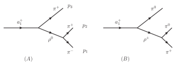
Figure 1: The dominant diagrams for the decay of $a_{1}(1260)\to 3\pi$. (A): $a^{+}_{1}(1260)\to\pi^{+}\pi^{+}\pi^{-}$ and (B): $a^{+}_{1}(1260)\to\pi^{+}\pi^{0}\pi^{0}$.

II.1 Decay amplitude at tree level

In order to evaluate the partial decay width of $a_{1}(1260)\to 3\pi$, we need the decay amplitudes of the tree level diagrams shown in Fig. 1, where the process is described as the $a_{1}(1260)$ decaying to $\rho\pi$ and then the $\rho$ decaying into $\pi\pi$. As mentioned above, $a_{1}(1260)$ results as dynamically generated from the interactions of the $\rho\pi$ and $\bar{K}K^{*}$ in coupled channels. We can write the $a^{+}_{1}\rho^{0}\pi^{+}$ vertex as

$$-it_{1}=-i\frac{g_{a_{1}\rho\pi}}{\sqrt{2}}\varepsilon_{a_{1}}^{\mu}\varepsilon_{\mu},$$ (1)

where $\varepsilon^{\mu}_{a_{1}}$ is the polarization vector of $a_{1}(1260)$ and $\varepsilon^{\mu}$ the polarization vector of the $\rho$. The $g_{a_{1}\rho\pi}$ is the coupling of the $a_{1}(1260)$ to the $\rho\pi$ channel and can be obtained from the residue in the pole of the scattering amplitude in $I=1$. We take $g_{a_{1}\rho\pi}=(-3795+i2330)$ and $g_{a_{1}\bar{K}K^{*}}=(1872-i1468)$ MeV as obtained in Ref. Roca:2005nm . We can see that the $a_{1}(1260)$ has large coupling to $\rho\pi$ channel comparing to the $\bar{K}K^{*}$ channel.

To compute the decay amplitude, we also need the structure of the $\rho\pi\pi$ vertices which can be evaluated by means of hidden gauge symmetry Lagrangian describing the vector-pseudoscalar-pseudoscalar ($VPP$) interaction Bando:1984ej ; Bando:1987br ; Meissner:1987ge ; Harada:2003jx , given by

$${{\cal L}_{VPP}}=-ig<V^{\mu}[P,\partial_{\mu}P]>,$$ (2)

where the symbol $<>$ stands for the trace in $SU(3)$ and $g=\frac{m_{V}}{2f}$, with $m_{V}=m_{\rho}$ and $f=93$ MeV the pion decay constant. The matrices $P$ and $V$ contain the nonet of the pseudoscalar mesons and the one of the vectors respectively.

From the Lagrangian of Eq. (2), the vertex of $\rho^{0}\pi^{+}\pi^{-}$ can be written as 

$${-it_{2}}=-ig\sqrt{2}(p_{1}-p_{2})_{\mu}\varepsilon^{\mu},$$ (3)

where $p_{1}$ and $p_{2}$ are the momenta of $\pi^{-}$ and $\pi^{+}$ mesons, respectively.

We can now straightforwardly construct the decay amplitude for $a^{+}_{1}(1260)\to\pi^{+}\pi^{+}\pi^{-}$ decay corresponding to the tree diagram shown in Fig. 1 (A):

$$t_{\text{tree}} = -g_{a_{1}\rho\pi}g\left(\frac{F_{\rho\pi\pi}(q^{2}_{1})(p_{1}-p_{2})_{\mu}}{q_{1}^{2}-m_{\rho}^{2}+im_{\rho}\Gamma_{\rho}(q^{2}_{1})}\right.$$ (5)

$$\left.+\frac{F_{\rho\pi\pi}(q^{2}_{2})(p_{1}-p_{3})_{\mu}}{q_{2}^{2}-m_{\rho}^{2}+im_{\rho}\Gamma_{\rho}(q^{2}_{2})}\right)\varepsilon_{a_{1}}^{\mu},$$

$$= g_{a_{1}\rho\pi}g\left(\frac{F_{\rho\pi\pi}(q^{2}_{1})(\vec{p}_{1}-\vec{p}_{2})}{q_{1}^{2}-m_{\rho}^{2}+im_{\rho}\Gamma_{\rho}(q^{2}_{1})}\right.$$

$$\left.+\frac{F_{\rho\pi\pi}(q^{2}_{2})(\vec{p}_{1}-\vec{p}_{3})}{q_{2}^{2}-m_{\rho}^{2}+im_{\rho}\Gamma_{\rho}(q^{2}_{2})}\right)\cdot\vec{\varepsilon}_{a_{1}},$$

where the two terms stand for the contributions with the $\rho^{0}$ in the $\pi^{-}_{1}\pi^{+}_{2}$ and in the $\pi^{-}_{1}\pi^{+}_{3}$ subsystem, and $q_{1}=p_{1}+p_{2}$ and $q_{2}=p_{1}+p_{3}$.

We take the energy dependent decay width of $\Gamma_{\rho}$. Because the dominant decay channel of $\rho$ is $\pi\pi$, we take

$$\Gamma_{\rho}(M^{2}_{\rm inv})=\Gamma_{{\rm on}}\left(\frac{q_{{\rm off}}}{q_{{\rm on}}}\right)^{3}\frac{m_{\rho}}{M_{\rm inv}},$$ (6)

with $\Gamma_{\rm on}=149.1$ MeV, and

$$q_{\rm on} = \frac{\sqrt{m^{2}_{\rho}-4m^{2}_{\pi}}}{2},$$ (7)

$$q_{\rm off} = \frac{\sqrt{M^{2}_{\rm inv}-4m^{2}_{\pi}}}{2},$$ (8)

with $M^{2}_{\rm inv}=M^{2}_{12}=q^{2}_{1}$ or $q^{2}_{2}$ the invariant mass square of the $\pi^{+}\pi^{-}$ system corresponding the two terms shown in Eq. (5). We take $m_{\rho}=775.26$ MeV in this work.

It is worthy to mention that the parametrization of the width of the $\rho$ meson shown in Eq. (6) is common and it is meant to take into account the phase space of each decay mode as a function of the energy Chiang:1990ft ; Xie:2007qt ; Hanhart:2010wh . In the present work we take explicitly the phase space for the $P$-wave decay of the $\rho$ into two pions.

Besides, in Eq. (5), $F_{\rho\pi\pi}$ is the form factor of $\rho^{0}$. In our present calculation we adopt the following form as used in previous works Tsushima:2000hs ; Gasparyan:2003fp ; Xie:2007vs ; Xie:2007qt ; Xie:2015wja

$$F_{\rho\pi\pi}(M^{2}_{\rm inv})=\frac{\Lambda_{\rho}^{4}}{\Lambda_{\rho}^{4}+(M^{2}_{\rm inv}-m_{\rho}^{2})^{2}},$$ (9)

where $\Lambda_{\rho}$ is the cutoff parameter of $\rho^{0}$.

II.2 Decay amplitude for the triangular loop

In addition to the tree level diagrams shown in Fig. 1, we study also the contributions of $\pi\pi\to\pi\pi$ and $K\bar{K}\to\pi\pi$ final state interaction (FSI). For this purpose, we use the triangular mechanism contained in the diagrams shown in Fig. 2, consisting in the rescatering of the $\pi\pi$ and $K\bar{K}$ pairs. The rescattering of $\pi\pi$ and $K\bar{K}$ in coupled channels dynamically generates the $f_{0}(500)$ and $f_{0}(980)$ resonances.

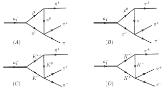
Figure 2: Triangular loop contributions to the $a^{+}_{1}(1260)\to\pi^{+}\pi^{-}\pi^{+}$ decay.

We can write explicitly the decay amplitudes for the triangular diagrams shown in Fig. 2 as (see also Ref. Aceti:2016yeb , where more details can be found)

$$t_{\rm{FSI}}^{A+B} = g_{a_{1}\rho\pi}g\left[(2I_{1}+I_{2})t_{\pi\pi\to\pi\pi}\vec{p}_{2}\cdot\vec{\varepsilon}_{a_{1}}\right.$$ (10)

$$\left.+(2I_{1}+I_{2})t_{\pi\pi\to\pi\pi}\vec{p}_{3}\cdot\vec{\varepsilon}_{a_{1}}\right],$$

$$t_{\rm{FSI}}^{C+D} = -\frac{g_{a_{1}\bar{K}K^{*}}g}{\sqrt{2}}\left[(2I^{\prime}_{1}+I^{\prime}_{2})t_{K\bar{K}\to\pi\pi}\vec{p}_{2}\cdot\vec{\varepsilon}_{a_{1}}\right.$$ (11)

$$\left.+(2I^{\prime}_{1}+I^{\prime}_{2})t_{K\bar{K}\to\pi\pi}\vec{p}_{3}\cdot\vec{\varepsilon}_{a_{1}}\right],$$

with

$$t_{\pi\pi\to\pi\pi} = \sqrt{2}t_{\pi^{0}\pi^{0}\to\pi^{+}\pi^{-}}+t_{\pi^{+}\pi^{-}\to\pi^{+}\pi^{-}},$$ (12)

$$t_{K\bar{K}\to\pi\pi} = t_{K^{0}\bar{K}^{0}\to\pi^{+}\pi^{-}}+t_{K^{+}K^{-}\to\pi^{+}\pi^{-}},$$ (13)

where $t_{\pi^{0}\pi^{0}\to\pi^{+}\pi^{-}}$, $t_{\pi^{+}\pi^{-}\to\pi^{+}\pi^{-}}$, $t_{K^{0}\bar{K}^{0}\to\pi^{+}\pi^{-}}$, and $t_{K^{+}K^{-}\to\pi^{+}\pi^{-}}$ are the meson-meson scattering amplitudes obtained in the chiral unitary approach in Ref. Oller:1997ti , which depend on the invariant mass of $\pi^{+}\pi^{-}$. The $t_{\pi\pi\to\pi\pi}$ and $t_{K\bar{K}\to\pi\pi}$ in the first and second terms in Eqs. (10) and (11) depend on $q^{2}_{2}$ and $q^{2}_{1}$, respectively. In addition, in Eq. (10) the quantities $I_{1}$ and $I_{2}$ are given by

$$I_{1} = -\int\frac{d^{3}q}{(2\pi)^{3}}\frac{1}{8\omega(q)\omega^{\prime}(q)\omega^{*}(q)}\frac{1}{k^{0}-\omega^{\prime}(q)-\omega^{*}(q)+i\epsilon}\frac{1}{P^{0}-\omega^{*}(q)-\omega(q)+i\epsilon}$$ (14)

$$\times\frac{2P^{0}\omega(q)+2k^{0}\omega^{\prime}(q)-2(\omega(q)+\omega^{\prime}(q))(\omega(q)+\omega^{\prime}(q)+\omega^{*}(q))}{(P^{0}-\omega(q)-\omega^{\prime}(q)-k^{0}+i\epsilon)(P^{0}+\omega(q)+\omega^{\prime}(q)-k^{0}-i\epsilon)},$$

$$I_{2} = -\int\frac{d^{3}q}{(2\pi)^{3}}\frac{\vec{k}\cdot\vec{q}/|\vec{k}|^{2}}{8\omega(q)\omega^{\prime}(q)\omega^{*}(q)}\frac{1}{k^{0}-\omega^{\prime}(q)-\omega^{*}(q)+i\epsilon}\,\frac{1}{P^{0}-\omega^{*}(q)-\omega(q)+i\epsilon}$$ (15)

$$\times\frac{2P^{0}\omega(q)+2k^{0}\omega^{\prime}(q)-2(\omega(q)+\omega^{\prime}(q))(\omega(q)+\omega^{\prime}(q)+\omega^{*}(q))}{(P^{0}-\omega(q)-\omega^{\prime}(q)-k^{0}+i\epsilon)(P^{0}+\omega(q)+\omega^{\prime}(q)-k^{0}-i\epsilon)},$$

with $k=p_{2}$ for the first term and $k=p_{3}$ for the second term in Eq. (10). While $\omega(q)=\sqrt{\vec{q}^{~{}2}+m^{2}_{\pi}}$, $\omega^{\prime}(q)=\sqrt{(\vec{q}+\vec{k})^{2}+m^{2}_{\pi}}$, and $\omega^{*}(q)=\sqrt{\vec{q}^{~{}2}+m^{2}_{\rho}}$ are the energies of the $\pi^{0}$ ($\pi^{+}$) and $\pi^{0}$ ($\pi^{-}$), and $\rho$ meson in the triangular loop, respectively. A more detailed derivation can be found in Refs. Aceti:2015zva ; Aceti:2015pma . Furthermore, $I^{\prime}_{1}$ and $I^{\prime}_{2}$ can easily be obtained just applying the substitution to $I_{1}$ and $I_{2}$ with $m_{\pi}\to m_{K}$ and $m_{\rho}\to m_{K^{*}}$.

It is worth mentioning that after performing the integrations, the $I_{1}$ and $I_{2}$ integrals in the above equations depend only on the modulus of the momentum of one of the outgoing $\pi^{+}$, which can be easily related to the invariant mass of the $\pi^{+}\pi^{-}$ system via $M^{2}_{\pi^{+}\pi^{-}}=M^{2}_{a_{1}}+m^{2}_{\pi}-2M_{a_{1}}\sqrt{|\vec{p}_{2}|^{2}+m^{2}_{\pi}}$ and $M^{2}_{\pi^{+}\pi^{-}}=M^{2}_{a_{1}}+m^{2}_{\pi}-2M_{a_{1}}\sqrt{|\vec{p}_{3}|^{2}+m^{2}_{\pi}}$ for the first and second terms in Eqs. (10) and (11), respectively. The $d^{3}q$ integrations are done with a cutoff $q_{\rm max}=630$ MeV.

III Numerical results and discussion

With the decay amplitudes obtained above, we can easily get the total decay width of $a_{1}(1260)\to 3\pi$ which is

$$d\Gamma=\frac{1}{192\pi^{3}M^{2}_{a_{1}}}{\sum}|t|^{2}p_{1}^{*}p_{3}dM_{12}d{\rm cos}\theta^{*},$$ (16)

where $t=t_{\rm tree}+t^{A+B}_{\rm FSI}+t^{C+D}_{\rm FSI}$ is the total decay amplitude for the decay of $a^{+}_{1}(1260)\to\pi^{+}\pi^{+}\pi^{-}$. The $p_{3}$ and $p_{1}^{*}$ are the three-momenta of the outgoing $\pi^{+}_{3}$ ($\pi^{+}_{2}$) meson in the $a^{+}_{1}(1260)$ rest frame and the outgoing $\pi^{-}$ meson in the center of mass frame of the final $\pi^{-}_{1}\pi^{+}_{2}$ ($\pi^{-}_{1}\pi^{+}_{3}$) system, respectively. They are given by

$$p_{3} = \frac{\lambda^{1/2}(M^{2}_{a_{1}},M^{2}_{12},m^{2}_{\pi})}{2M_{a_{1}}},$$ (17)

$$p^{*}_{1} = \frac{\lambda^{1/2}(M^{2}_{12},m^{2}_{\pi},m^{2}_{\pi})}{2M_{12}},$$ (18)

where $\lambda(x,y,z)$ is the Kählen or triangle function. We take $m_{\pi}=139.57$ MeV in this calculation.

For $\sum|t|^{2}$, the sum over polarizations can be easily done thanks to

$$\sum\varepsilon_{a_{1}}^{\mu}\varepsilon^{\nu*}_{a_{1}} = -g^{\mu\nu}+\frac{q^{\mu}q^{\nu}}{M^{2}_{a_{1}}},$$ (19)

with $q$ the four-momentum of the $a_{1}(1260)$. Here we give explicitly the results for the tree diagrams, as an example,

$$\sum|t_{\rm tree}|^{2}=g^{2}_{a_{1}\rho\pi}g^{2}\left(\frac{(E_{1}-E_{2})^{2}-(p_{1}-p_{2})^{2}}{D_{1}}\right.$$

$$\left.+\frac{(E_{3}-E_{2})^{2}-(p_{3}-p_{2})^{2}}{D_{2}}+\right.$$

$$\left.\!\!\!\!\!\frac{(E_{1}-E_{2})(E_{3}-E_{2})-(p_{1}-p_{2})\cdot(p_{3}-p_{2})}{D_{3}}\right),$$ (20)

with

$$D_{1} = (q_{1}^{2}-m^{2}_{\rho})^{2}+[m_{\rho}\Gamma_{\rho}(q_{1}^{2})]^{2},$$ (21)

$$D_{2} = (q_{2}^{2}-m^{2}_{\rho})^{2}+[m_{\rho}\Gamma_{\rho}(q_{2}^{2})]^{2},$$ (22)

$$D_{3} = \frac{1}{2}\frac{D_{1}D_{2}}{(q^{2}_{1}-m^{2}_{\rho})(q^{2}_{2}-m^{2}_{\rho})+m^{2}_{\rho}\Gamma_{\rho}(q_{1}^{2})\Gamma_{\rho}(q_{2}^{2})},$$ (23)

and

$$E_{3}=\frac{M^{2}_{a_{1}}+m^{2}_{\pi}-M^{2}_{12}}{2M_{a_{1}}},$$ (24)

$$E_{1}=\frac{M_{a_{1}}-E_{3}}{2}-\frac{p_{3}p^{*}_{1}}{M_{12}}{\rm cos}\theta^{*},$$ (25)

$$E_{2}=\frac{M_{a_{1}}-E_{3}}{2}+\frac{p_{3}p^{*}_{1}}{M_{12}}{\rm cos}\theta^{*},$$ (26)

$$(p_{1}-p_{2})^{2}=4m^{2}_{\pi}-M^{2}_{12},$$ (27)

$$(p_{3}-p_{2})^{2}=3m^{2}_{\pi}-M_{a_{1}}E_{3}-\frac{2M_{a_{1}}p_{3}p^{*}_{1}{\rm cos}\theta^{*}}{M_{12}},$$ (28)

$$(p_{1}-p_{2})\cdot(p_{3}-p_{2})=\frac{M^{2}_{a_{1}}+m^{2}_{\pi}}{2}-2M_{a_{1}}E_{2}.$$ (29)

The range of $M_{12}$ is

$$M^{\rm max}_{12} = M_{a_{1}}-m_{\pi},$$

$$M^{\rm min}_{12} = 2m_{\pi}.$$

With all the ingredients obtained above, one can easily get the total decay width of $a_{1}(1260)\to 3\pi$ by performing the integration of $M_{12}$ and ${\rm cos}\theta^{*}$. The results for $\Gamma$ as a function of $\Lambda_{\rho}$ is shown in Fig. 3 with $M_{a_{1}}=1230$ MeV. From Fig. 3 one can see that the results for $\Gamma$ are not sensitive to the value of $\Lambda_{\rho}$, therefore, we fix $\Lambda_{\rho}=1500$ MeV in the next calculations.

Figure 3: The total decay width of $a_{1}(1260)\to 3\pi$ as a function of the cutoff parameter $\Lambda_{\rho}$.

However, since $a_{1}(1260)$ has large total decay width which should be taken into account. For this purpose we replace the $d\Gamma$ in Eq. (16) by $d\tilde{\Gamma}$:

$$d\tilde{\Gamma}=\int^{(M_{a_{1}}+2\Gamma_{a_{1}})^{2}}_{(M_{a_{1}}-2\Gamma_{a_{1}})^{2}}d\Gamma dm^{2}S(m^{2}),$$ (30)

where the spectral function $S(m^{2})$ is defined as

$$S(m^{2})=-\frac{1}{\pi}{\rm Im}\left(\frac{1}{m^{2}-M^{2}_{a_{1}}+iM_{a_{1}}\Gamma_{a_{1}}}\right).$$ (31)

In Fig. 4, we show the numerical results for $\pi^{+}\pi^{-}$ invariant mass distributions. We compare also our theoretical calculations with the experimental results of Ref. Albrecht:1992ka measured in the decay of $\tau\to\pi^{-}\pi^{-}\pi^{+}\nu_{\tau}$. In Fig. 4 we see that the tree level alone can describe well the experimental data around the $\rho$ peak. This is attributed to the effect of the $\rho^{0}$ off shell propagator. The implementation of the contributions of the triangle loop diagrams is responsible for the enhancement of the invariant mass distribution at the lower invariant masses, where the $f_{0}(500)$ resonance appears. There is also a small peak around the $K\bar{K}$ mass threshold, where the $f_{0}(980)$ resonance appears.

Figure 4: The $\pi^{+}\pi^{-}$ invariant mass distribution for $a_{1}(1260)\to 3\pi$ as a function of the invariant mass of the $\pi^{+}\pi^{-}$ system. The experimental data are taken from Ref. Albrecht:1992ka .

The numerical results in Fig. 4 show how the most drastic change in the line shape of the the invariant $\pi^{+}\pi^{-}$ mass distribution is caused by the tree diagram alone in Fig. 1 and, as mentioned before, this is tied to the $\rho^{0}$ contribution, which appears at tree level because of the large coupling of $a_{1}(1260)$ to $\rho\pi$ channel obtained in the chiral unitary approach Roca:2005nm .

Figure 5: The total decay width of $a_{1}(1260)\to 3\pi$ as a function of $M_{a_{1}}$.

Next, we calculate the total decay width of $a^{+}_{1}(1260)\to\pi^{+}\pi^{+}\pi^{-}$ as a function of the mass of $a_{1}(1260)$. The numerical result is shown in Fig. 5. The width rises rapidly with increasing $M_{a_{1}}$ in the mass range $M_{a_{1}}<1300$ MeV, while it goes to flat when $M_{a_{1}}>1400$ MeV. Besides, we get $\Gamma=166$ MeV at $M_{a_{1}}=1230$ MeV. There is still no precise measurement about the $a^{+}_{1}(1260)\to\pi^{+}\pi^{+}\pi^{-}$ decay, we cannot compare our result with experiment. Note that the width $\Gamma_{a_{1}}\equiv\Gamma_{a^{0}_{1}\to\pi^{+}\pi^{-}\pi^{0}}$ was studied in Ref. Achasov:2004re , and $\Gamma_{a_{1}}=860$ MeV was obtained at $M_{a_{1}}=1230$ MeV. One can see that the theoretical result in Ref. Achasov:2004re is much different with us. On the other hand, there are two peaks in the solid curve in Fig. 5, which are attributed to the effect of the $\pi\pi\to\pi\pi$ and $K\bar{K}\to\pi\pi$ final state interactions. We hope that the future experiments could test the model calculations.

So far we have assumed that the $a_{1}(1260)$ resonance is fully made from $\rho\pi$ and $\bar{K}K^{*}$ interaction. The pole position $(M^{\rm pole}_{a_{1}}-i\Gamma^{\rm pole}_{a_{1}}/2)$ is identified from the zero of the denominator of the scattering amplitudes in the complex plane, and the effective couplings $g_{a_{1}\rho\pi}$ and $g_{a_{1}\bar{K}K^{*}}$ are calculated from the residues of the scattering amplitudes at the complex pole. We know that the $a_{1}(1260)$ Breit-Wigner parameters, $M_{a_{1}}$ and $\Gamma_{a_{1}}$, deviate from its pole parameters by a large amount and are reaction dependent Patrignani:2016xqp . On the other hand, we have no information on how the effective couplings obtained at the pole position change with varying $M_{a_{1}}$, and therefore, we cannot include the uncertainties of these effective couplings without making further assumptions. Besides, there are hints that the $a_{1}(1260)$ resonance could have also other components as mention above, thus, there should be also contribution from $a_{1}(1260)\to f_{0}(500)\pi\to 3\pi$ Patrignani:2016xqp in the tree level. However, the information about this contribution is very scarce. We will leave such studies to a future work.

IV summary

In this work, we evaluate the partial decay width of the $a^{+}_{1}(1260)\to\pi^{+}\pi^{+}\pi^{-}$ with the assumption that the $a_{1}(1260)$ is dynamically generated from the coupled channel $\rho\pi$ and $\bar{K}K^{*}$ interactions. The dominant tree level diagrams that proceed via $a^{+}_{1}(1260)\to\rho^{0}\pi^{+}\to\pi^{+}\pi^{+}\pi^{-}$ are considered. Besides, we also take into account the final state interactions of $\pi\pi\to\pi\pi$ and $K\bar{K}\to\pi\pi$. It is found that the contributions from $\pi\pi\to\pi\pi$ and $K\bar{K}\to\pi\pi$ are small compare to the tree level diagram, but they change the $\pi^{+}\pi^{-}$ invariant mass distributions of the $a_{1}(1260)\to 3\pi$ decay.

The results that we obtained for the $\pi^{+}\pi^{-}$ invariant mass distributions are in a fair agreement with the experimental measurements for the $\tau\to\pi^{-}\pi^{-}\pi^{+}\nu_{\tau}$ decay. This provides new support for the molecular picture of $a_{1}(1260)$. Furthermore, we calculate also the total decay width as a function of the mass of $a_{1}(1260)$, it is found that our result is different with other model calculations. Thus, we hope that the further experimental observations of the $\pi^{+}\pi^{-}$ and $\pi^{+}\pi^{+}\pi^{-}$ mass distributions would then test these model calculations and provide vary valuable information on the relevance of the $\rho\pi$ component in the $a_{1}(1260)$ wave function.

References

- (1) C. Patrignani et al. [Particle Data Group], Chin. Phys. C 40, 100001 (2016).
- (2) E. Klempt and A. Zaitsev, Phys. Rept. 454, 1 (2007).
- (3) N. Brambilla et al., Eur. Phys. J. C 74, 2981 (2014).
- (4) V. Baru, J. Haidenbauer, C. Hanhart, Y. Kalashnikova and A. E. Kudryavtsev, Phys. Lett. B 586, 53 (2004).
- (5) T. Hyodo, D. Jido and A. Hosaka, Phys. Rev. C 78, 025203 (2008).
- (6) L. Roca, E. Oset and J. Singh, Phys. Rev. D 72, 014002 (2005).
- (7) L. Roca, A. Hosaka and E. Oset, Phys. Lett. B 658, 17 (2007).
- (8) H. Nagahiro, L. Roca, A. Hosaka and E. Oset, Phys. Rev. D 79, 014015 (2009).
- (9) C. B. Lang, L. Leskovec, D. Mohler and S. Prelovsek, JHEP 1404, 162 (2014).
- (10) Y. Zhou, X. L. Ren, H. X. Chen and L. S. Geng, Phys. Rev. D 90, 014020 (2014).
- (11) M. F. M. Lutz and E. E. Kolomeitsev, Nucl. Phys. A 730, 392 (2004).
- (12) S. Weinberg, Phys. Rev. Lett. 18, 507 (1967).
- (13) C. W. Bernard, A. Duncan, J. LoSecco and S. Weinberg, Phys. Rev. D 12, 792 (1975).
- (14) G. Ecker, J. Gasser, A. Pich and E. de Rafael, Nucl. Phys. B 321, 311 (1989).
- (15) D. Gomez Dumm, A. Pich and J. Portoles, Phys. Rev. D 69, 073002 (2004).
- (16) M. Wagner and S. Leupold, Phys. Rev. D 78, 053001 (2008).
- (17) D. G. Dumm, P. Roig, A. Pich and J. Portoles, Phys. Lett. B 685, 158 (2010).
- (18) I. M. Nugent, T. Przedzinski, P. Roig, O. Shekhovtsova and Z. Was, Phys. Rev. D 88, 093012 (2013).
- (19) N. N. Achasov and A. A. Kozhevnikov, Phys. Rev. D 71, 034015 (2005).
- (20) P. Lichard and J. Juran, Phys. Rev. D 76, 094030 (2007).
- (21) C. Cheng, J. J. Xie and X. Cao, Commun. Theor. Phys. 66, 675 (2016).
- (22) H. Nagahiro, K. Nawa, S. Ozaki, D. Jido and A. Hosaka, Phys. Rev. D 83, 111504 (2011).
- (23) L. S. Geng, E. Oset, J. R. Pelaez and L. Roca, Eur. Phys. J. A 39, 81 (2009).
- (24) Z. H. Guo and J. A. Oller, Phys. Rev. D 93, 096001 (2016).
- (25) M. Bando, T. Kugo and K. Yamawaki, Phys. Rept. 164, 217 (1988).
- (26) N. Kaiser and U. G. Meissner, Nucl. Phys. A 519, 671 (1990).
- (27) T. Sakai and S. Sugimoto, Prog. Theor. Phys. 113, 843 (2005).
- (28) T. Sakai and S. Sugimoto, Prog. Theor. Phys. 114, 1083 (2005).
- (29) M. Alekseev et al. [COMPASS Collaboration], Phys. Rev. Lett. 104, 241803 (2010).
- (30) D. M. Asner et al. [CLEO Collaboration], Phys. Rev. D 61, 012002 (2000).
- (31) R. A. Briere et al. [CLEO Collaboration], Phys. Rev. Lett. 90, 181802 (2003).
- (32) T. E. Coan et al. [CLEO Collaboration], Phys. Rev. Lett. 92, 232001 (2004).
- (33) R. R. Akhmetshin et al. [CMD-2 Collaboration], Phys. Lett. B 466, 392 (1999).
- (34) P. Salvini et al. [OBELIX Collaboration], Eur. Phys. J. C 35, 21 (2004).
- (35) M. Bando, T. Kugo, S. Uehara, K. Yamawaki and T. Yanagida, Phys. Rev. Lett. 54, 1215 (1985).
- (36) U. G. Meißner, Phys. Rept. 161, 213 (1988).
- (37) M. Harada and K. Yamawaki, Phys. Rept. 381, 1 (2003).
- (38) J. J. Xie, C. Wilkin and B. S. Zou, Phys. Rev. C 77, 058202 (2008).
- (39) H. C. Chiang, E. Oset and L. C. Liu, Phys. Rev. C 44, 738 (1991).
- (40) C. Hanhart, Y. S. Kalashnikova and A. V. Nefediev, Phys. Rev. D 81, 094028 (2010).
- (41) J. J. Xie, B. S. Zou and H. C. Chiang, Phys. Rev. C 77, 015206 (2008).
- (42) K. Tsushima, A. Sibirtsev and A. W. Thomas, Phys. Rev. C 62, 064904 (2000).
- (43) A. M. Gasparyan, J. Haidenbauer, C. Hanhart and J. Speth, Phys. Rev. C 68, 045207 (2003).
- (44) J. J. Xie and B. S. Zou, Phys. Lett. B 649, 405 (2007).
- (45) J. J. Xie, Phys. Rev. C 92, 065203 (2015).
- (46) F. Aceti, L. R. Dai and E. Oset, Phys. Rev. D 94, 096015 (2016).
- (47) J. A. Oller and E. Oset, Nucl. Phys. A 620, 438 (1997) Erratum: [Nucl. Phys. A 652, 407 (1999)].
- (48) F. Aceti, J. M. Dias and E. Oset, Eur. Phys. J. A 51, 48 (2015).
- (49) F. Aceti, J. J. Xie and E. Oset, Phys. Lett. B 750, 609 (2015).
- (50) H. Albrecht et al. [ARGUS Collaboration], Z. Phys. C 58, 61 (1993).