Two-Scalar Turbulent Rayleigh-Bénard Convection: Numerical Simulations and Unifying Theory

Abstract

We conduct direct numerical simulations for turbulent Rayleigh-Bénard (RB) convection, driven simultaneously by two scalar components (say, temperature and salt concentration) with different molecular diffusivities, and measure the respective fluxes and the Reynolds number. To account for the results, we generalize the Grossmann-Lohse theory for traditional RB convections (Grossmann and Lohse, J. Fluid Mech., 407, 27-56; Phys. Rev. Lett., 86, 3316-3319; Stevens et al., J. Fluid Mech., 730, 295-308) to this two-scalar turbulent convection. Our numerical results suggest that the generalized theory can successfully predict the overall trends for the fluxes of two scalars and the Reynolds number. In fact, for most of the parameters explored here, the theory can even predict the absolute values of the fluxes and the Reynolds number with good accuracy. The current study extends the generality of the Grossmann-Lohse theory in the area of the buoyancy-driven convection flows.

I Introduction

Rayleigh-Bénard (RB) convection serves as a commonly used system for studying natural convection which is ubiquitous in many nature and engineering environments. RB convection refers to a fluid layer which is heated from below and cooled from above, and is subject to an external gravitation field. Such systems have been extensively studied in recent years, e.g. see the reviews of Ahlers et al. (2009), Lohse & Xia (2010), and Chillà & Schumacher (2012). One key question is how the scalar flux and flow velocity depend on the control parameters. The unifying theory for the flux and flow velocity (“GL theory” Grossmann & Lohse, 2000, 2001, 2002, 2004), which are measured respectively by the Nusselt number Nu and the Reynolds number Re, has achieved great success for RB flows (Ahlers et al., 2009; Stevens et al., 2013), and now has predictive power for the absolute values of Nu and Re for given control parameters, i.e. the Rayleigh number Ra and the Prandtl number Pr.

However, in reality the convection flow can be much more complex than the idealized RB system, as in the case of external rotation (e.g. King et al., 2009; Wei et al., 2015), inhomogeneities of the top and bottom boundaries (e.g. Wang et al., 2017; Bakhuis et al., 2018), or wall roughness (e.g. Shishkina & Wagner, 2011; Salort et al., 2014; Xie & Xia, 2017; Zhu et al., 2017). In this study we will investigate another type of complexity, i.e. RB convection driven by two different scalar components. Multiple-component convection is commonly encountered in nature. For instance, the density of seawater is mainly determined by temperature and salinity, and chemical reaction flows usually have more than one species. In the Ocean the vertical convection flow driven by both temperature and salinity gradients is usually referred to as double diffusive convection (DDC) (Turner, 1985; Radko, 2013). Our previous study on DDC was confined in the so-called fingering regime, where the fluid layer experiences an unstable salinity gradient and stable temperature gradient (Yang et al., 2015, 2016).

Here we will focus on the convection flow driven simultaneously by two scalar components with different molecular diffusivities. Our previous study showed that the original GL model can be used to describe the salinity transfer in fingering DDC flow (Yang et al., 2015, 2016). The theory has also been applied to DDC in the diffusive regime, in which the fluid layer is subjected to an unstable temperature gradient and a stable salinity gradient (Hieronymus & Carpenter, 2016). In this study the RB convection is driven by two scalar components which are both unstably stratified. Recall that the key idea of the GL theory is to divide both the momentum and thermal fields into their own boundary layer and bulk regions. Then scalings are developed for the two respective contributions to the respective dissipation rates, leading to $\mbox{{Nu}}(\mbox{{Ra}},~{}\mbox{{Pr}})$ and $\mbox{{Re}}(\mbox{{Ra}},~{}\mbox{{Pr}})$. It is straightforward to generalize this type of argument to multiple scalar fields. We will validate this generalization of the GL theory by direct numerical simulations.

The paper is organized as follows. In section 2 we will provide the governing dynamical equations of the system and the details of our simulations. In section 3 we will present the generalization and application of the GL theory to the two-scalar RB convection. Finally section 4 concludes the paper.

II Governing equations and numerical simulations

The flow under consideration is incompressible and the density $\rho$ is determined by two scalar components, say temperature $\theta(\textbf{x},t)$ and concentration field $s(\textbf{x},t)$. The Oberbeck-Buossinesq approximation is adopted, i.e. the fluid density depends linearly on both scalars as $\rho(\theta,s)=\rho_{0}[1-\beta_{\theta}\theta+\beta_{s}s]$. $\rho_{0}$ is a reference density, while $\theta$ and $s$ are the temperature and concentration relative to their respective reference values. $\beta_{\zeta}$ is the positive expansion coefficient respectively for temperature ($\zeta=\theta$) and concentration ($\zeta=s$). From now on the subscript $\zeta=\theta$ or $s$ stands for a quantity associated to scalar $\zeta$. The signs before the two terms indicate that the density is bigger for either lower temperature or higher concentration, which are the usually cases in practice.

The governing equations consist of the momentum equation and the advection-diffusion equations of two scalars, which read

$$\partial_{t}u_{i}+u_{j}\partial_{j}u_{i}=-\partial_{i}p+\nu\partial_{j}^{2}u_{i}+g\delta_{i3}(\beta_{\theta}\theta-\beta_{s}s),$$ (1a)

$$\partial_{t}\theta+u_{j}\partial_{j}\theta=\kappa_{\theta}\partial_{j}^{2}\theta,$$ (1b)

$$\partial_{t}s+u_{j}\partial_{j}s=\kappa_{s}\partial_{j}^{2}s.$$ (1c)

Here $u_{i}$ with $i=1,~{}2,~{}3$ are three velocity components, $p$ is the kinematic pressure, $\nu$ is the kinematic viscosity, $g$ is the gravitational acceleration, and $\kappa_{\zeta}$ is the molecular diffusivity, respectively. The dynamic system is further constrained by the continuity equation $\partial_{i}u_{i}=0$.

The fluid layer is between two parallel plates which are perpendicular to gravity and separated by a height $H$. At each plate both the temperature and concentration are kept constant, and the scalar difference between two plates is denoted by $\Delta$. The top plate has lower temperature and higher concentration, thus the flow is driven by both scalars. The flow has four control parameters, namely two Prandtl numbers and two Rayleigh numbers,

$$\mbox{{Pr}}_{\zeta}=\frac{\nu}{\kappa_{\zeta}},\quad\quad\mbox{{Ra}}_{\zeta}=\frac{g\beta_{\zeta}\Delta_{\zeta}H^{3}}{\kappa_{\zeta}\nu}.$$ (2)

Another useful parameter, which is borrowed from the DDC community, is the density ratio

$$\Lambda=\frac{\beta_{\theta}\Delta_{\theta}}{\beta_{s}\Delta_{s}}=\frac{\mbox{{Pr}}_{s}\mbox{{Ra}}_{\theta}}{\mbox{{Pr}}_{\theta}\mbox{{Ra}}_{s}}.$$ (3)

$\Lambda$ measures the relative strength of the buoyancy force induced by the temperature difference to that induced by the concentration difference. $\Lambda<1$ indicates that the buoyancy force of the concentration difference is stronger than that of the temperature field, which we refer to as the “concentration-dominant” (CD) regime. Accordingly, $\Lambda>1$ is referred to as the “temperature-dominant” (TD) regime. Three key responses of the system are the scalar fluxes and the flow velocity, which are measured by the two Nusselt numbers and the Reynolds number

$$\mbox{{Nu}}_{s}=\frac{\langle u_{3}s\rangle-\kappa_{s}\partial_{3}\langle s\rangle}{\kappa_{s}\Delta_{s}H^{-1}},\quad\quad\mbox{{Nu}}_{\theta}=\frac{\langle u_{3}\theta\rangle-\kappa_{\theta}\partial_{3}\langle\theta\rangle}{\kappa_{\theta}\Delta_{\theta}H^{-1}},\quad\quad\mbox{{Re}}=\frac{u_{rms}H}{\nu}.$$ (4)

Here $\langle\cdot\rangle$ represents the spatial and time average. $u_{rms}$ is the root-mean-square value of the velocity magnitude.

The governing equation (1) is numerically solved by using a highly efficient code developed in our group (Ostilla-Mónico et al., 2015), which has been used intensively in our previous DDC studies (Yang et al., 2015, 2016). The code employs a multiple-grid method, which solves the momentum and fast-diffusing scalar on a base mesh, and the slow diffusing scalar on a refined mesh, respectively. The resolution is chosen to meet the criteria proposed in Stevens et al. (2010). The flow quantities are non-dimensionalized by the height $H$, the free-fall velocity defined by concentration difference $U_{c}=\sqrt{g\beta_{s}\Delta_{s}H}$, and the scalar differences $\Delta_{\zeta}$, respectively. At two plates no-slip boundary conditions are applied and both scalars are kept constant. In the two horizontal directions the periodic boundary conditions are employed. We fix $\mbox{{Pr}}_{\theta}=1$ and change $\mbox{{Ra}}_{\theta}$, $\mbox{{Ra}}_{s}$, and $\mbox{{Pr}}_{s}$. In this work we always set $\mbox{{Pr}}_{s}>\mbox{{Pr}}_{\theta}$, which implies that concentration diffuses slower than temperature. The simulated cases are summarized in table 1. All cases are sorted into four groups, as shown in table 1. Within each group we only vary one control parameter and fix all others constant.

$\mbox{{Pr}}_{s}$	$\mbox{{Ra}}_{\theta}$	$\mbox{{Ra}}_{s}$	$\Lambda$	$\Gamma$	$n_{x}$ ($m_{x}$)	$n_{z}$ ($m_{z}$)	$\mbox{{Nu}}_{\theta}$	$\mbox{{Nu}}_{s}$	Re
10.0	$10^{6}$	$10^{5}$	100.0	4.0	240(3)	128(2)	18.481	8.2880	221.24
10.0	$10^{6}$	$10^{6}$	10.0	4.0	240(3)	128(2)	18.737	8.3676	223.03
10.0	$10^{6}$	$10^{7}$	1.0	4.0	240(4)	192(2)	20.809	8.9735	238.63
10.0	$10^{6}$	$10^{8}$	0.1	4.0	288(4)	192(2)	31.683	12.456	395.77
10.0	$10^{6}$	$10^{9}$	0.01	4.0	512(4)	384(2)	60.811	22.773	1083.3
10.0	$10^{7}$	$10^{5}$	1000.0	4.0	384(4)	192(2)	35.609	15.769	681.74
10.0	$10^{7}$	$10^{6}$	100.0	4.0	384(4)	192(2)	35.723	15.841	680.93
10.0	$10^{7}$	$10^{7}$	10.0	4.0	384(4)	192(2)	36.131	15.946	687.62
10.0	$10^{7}$	$10^{8}$	1.0	4.0	384(4)	192(2)	40.168	17.152	744.13
10.0	$10^{7}$	$10^{9}$	0.1	2.0	288(4)	288(2)	63.993	24.929	1208.2
10.0	$10^{4}$	$10^{7}$	0.01	4.0	256(2)	192(1)	16.289	6.0401	99.597
10.0	$10^{5}$	$10^{7}$	0.1	4.0	256(2)	192(1)	16.714	6.5328	119.79
10.0	$10^{6}$	$10^{7}$	1.0	4.0	240(4)	192(2)	20.809	8.9735	238.63
10.0	$10^{7}$	$10^{7}$	10.0	4.0	384(4)	192(2)	36.131	15.946	687.62
10.0	$10^{8}$	$10^{7}$	100.0	2.0	384(4)	384(2)	72.405	31.514	1937.7
1.0	$10^{7}$	$10^{7}$	1.0	4.0	384(1)	192(1)	19.341	19.341	949.51
2.0	$10^{7}$	$10^{7}$	2.0	4.0	384(2)	192(1)	22.759	17.340	779.04
5.0	$10^{7}$	$10^{7}$	5.0	4.0	384(3)	192(2)	29.362	16.229	705.87
10.0	$10^{7}$	$10^{7}$	10.0	4.0	384(4)	192(2)	36.131	15.946	687.62
30.0	$10^{7}$	$10^{7}$	30.0	2.0	384(6)	385(2)	52.525	16.503	692.06

Table 1: Summary of the control parameters, numerical details, and the global responses. For all cases $\mbox{{Pr}}_{\theta}=1$. Columns from left to right: Prandtl number of concentration field, Rayleigh numbers of temperature and concentration, density ratio, aspect ratio of domain (horizontal length over height), horizontal resolution of base mesh (refinement factor of refined mesh), vertical resolution of base mesh (refinement factor of refined mesh), two Nusselt numbers, and Reynolds number. Note that some cases appear repeatedly for the completeness of each group.

In figure 1 we show the scalar fields of three different runs with fixed $\mbox{{Pr}}_{s}=10$ and $\mbox{{Ra}}_{s}=10^{7}$ but different $\mbox{{Ra}}_{\theta}=10^{5}$ (a, b), $10^{6}$ (c, d), and $10^{7}$ (e, f), or equivalently $\Lambda=0.1$, $1$, and $10$, respectively. For the case shown in figures 1(a, b) with $\Lambda=0.1$ the buoyancy force is dominated by the concentration difference. Since for this case the molecular diffusivity of temperature is ten times faster than that of concentration, the typical size of the temperature plumes is much larger than the concentration ones due to the fast horizontal diffusion. On the contrary, for $\Lambda=10$ as shown in figures 1(e, f) the temperature component contributes the most part of the buoyancy force, and the temperature plumes are very active. Now the concentration plumes become thin filaments embedded within temperature plumes. When $\Lambda=1$ (figures 1c, d) the two scalar components contribute equally to the total buoyancy force, and the size of the scalar plumes is in between of the other two cases.

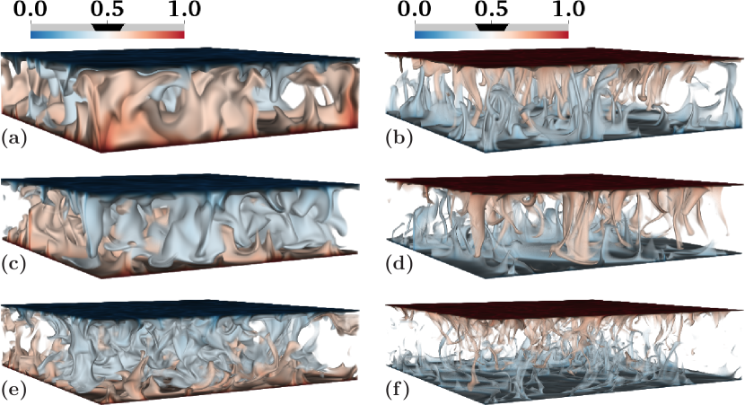
Figure 1: Three-dimensional volume rendering of the temperature (left column) and the concentration (right column) for three different runs with $\mbox{{Pr}}_{s}=10$ and $\mbox{{Ra}}_{s}=10^{7}$. From top row to bottom $\mbox{{Ra}}_{\theta}=10^{5}$, $10^{6}$, and $10^{7}$, or equivalently $\Lambda=0.1$, $1$, and $10$, respectively.

Figure 2 displays the profiles of the flow quantities for the three cases shown in figure 1. The mean profiles of the scalars suggest that both scalar fields have two thin boundary layer regions with high gradient adjacent to the plates, and in between a well mixed bulk region with nearly constant mean values (see figures 2a, 2c, 2e). In figures 2b, 2d, and 2f we plot the root-mean-square (rms) profiles of the fluctuations of scalars and one horizontal velocity component near the bottom plate. As in the RB flow, the peak location in rms profile can be regarded as the height of the boundary layers. Note that for the three cases shown here, $\mbox{{Ra}}_{s}$ is fixed at $10^{7}$, and $\mbox{{Ra}}_{\theta}$ increases from $10^{5}$ to $10^{7}$. As $\mbox{{Ra}}_{\theta}$ becomes larger, the total driving buoyancy force increases. The velocity fluctuation becomes stronger, indicating more intense turbulence. Accordingly, the peak location of velocity rms moves closer to the plate. Meanwhile, the boundary layer thickness of both scalars decreases and the concentration boundary layer is always nested inside the temperature boundary layer due to its smaller diffusivity than that of temperature.

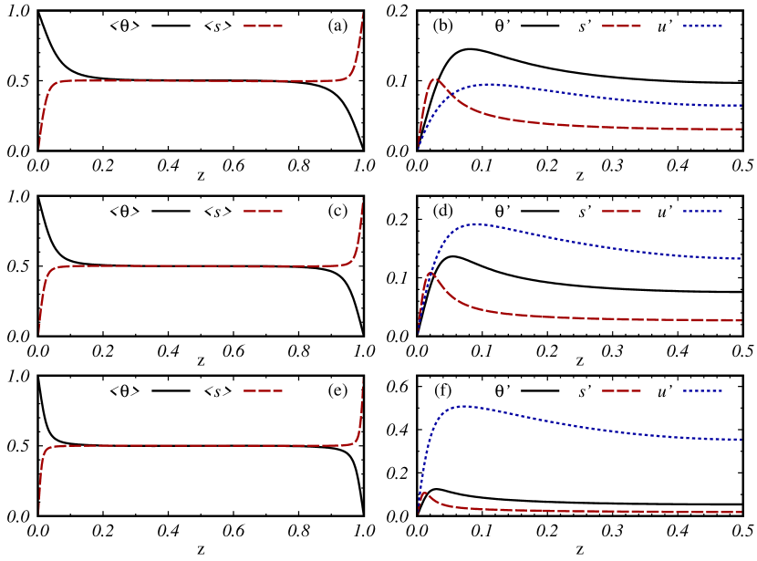
Figure 2: Mean profiles of two scalars (left column) and the root-mean-square of scalars and one horizontal velocity coponent (right column) for the three cases shown in figure 1 (from top to bottom). For clarity of the near wall region and due to the symmetry about $z=0.5$, in the right column we only show the lower half of the domain.

Interestingly, the momentum boundary layer has larger thickness than both scalar fields, even for the case with $\mbox{{Ra}}_{\theta}=10^{5}$ shown in figure 2b. Note that for this case $\Lambda=0.1$, meaning that the buoyancy force of the temperature difference is much smaller than that of the concentration difference. But the momentum boundary layer thickness is still set by the temperature field. This is consistent with the flow structures shown in figure 1, since temperature diffuses faster than concentration and its boundary layer extends beyond that of concentration field. Thermal plumes grow from a location higher than concentration plumes do and therefore the temperature field sets the momentum boundary layer height even for very small $\Lambda$.

III Generalized Grossmann-Lohse theory

The GL theory was originally developed for RB flow (Grossmann & Lohse, 2000, 2001, 2002, 2004) to provide a unifying theory for $\mbox{{Nu}}(\mbox{{Ra}},~{}\mbox{{Pr}})$ and $\mbox{{Re}}(\mbox{{Ra}},~{}\mbox{{Pr}})$, and successfully accounts for most of the existing experimental and numerical results (Ahlers et al., 2009; Stevens et al., 2013). Our previous DDC studies (Yang et al., 2015, 2016) showed that the original theory, without any modification of the coefficients, can also be used to describe the concentration flux and flow velocity scalings of the fingering DDC flow, i.e. flow driven by a concentration difference and stablized by a temperature difference. In this section we will briefly discuss the theory and the formulations, and then apply it to the current two-scalar convection flow.

The theory is built upon the exact relations between the dissipation rates and the global fluxes, which for the present problem read

$$\epsilon_{\theta} \equiv \left\langle\kappa_{\theta}[\partial_{i}\theta]^{2}\right\rangle_{V}=\kappa_{\theta}\,(\Delta_{\theta})^{2}\,H^{-2}\,\mbox{{Nu}}_{\theta},$$ (5a)

$$\epsilon_{s} \equiv \left\langle\kappa_{s}[\partial_{i}s]^{2}\right\rangle_{V}=\kappa_{s}\,(\Delta_{s})^{2}\,H^{-2}\,\mbox{{Nu}}_{s},$$ (5b)

$$\epsilon_{u} \equiv \left\langle\nu[\partial_{i}u_{j}]^{2}\right\rangle_{V}=\nu^{3}H^{-4}\,\left[\mbox{{Ra}}_{\theta}\,\mbox{{Pr}}^{-2}_{\theta}(\mbox{{Nu}}_{\theta}-1)+\mbox{{Ra}}_{s}\,\mbox{{Pr}}^{-2}_{s}(\mbox{{Nu}}_{s}-1)\right].$$ (5c)

The flow domain is divided into the boundary-layer and bulk regions. For each region different scalings are derived for the individual dissipation rates. Such division is still applicable to the current flow, as shown in figure 1. Following the same arguments as in the original theory, one finally obtains the GL theory for the turbulent two-scalar convective flow, namely

$$(\mbox{{Nu}}_{s}-1)\mbox{{Ra}}_{s}\mbox{{Pr}}_{s}^{-2}+(\mbox{{Nu}}_{\theta}-1)\mbox{{Ra}}_{\theta}\mbox{{Pr}}_{\theta}^{-2}=c_{1}\frac{\mbox{{Re}}^{2}}{g\left(\sqrt{\mbox{{Re}}_{c}/\mbox{{Re}}}\right)}+c_{2}\mbox{{Re}}^{3},$$ (6a)

$$\mbox{{Nu}}_{\theta}-1=c_{3}\mbox{{Re}}^{1/2}\,\mbox{{Pr}}_{\theta}^{1/2}\left\{f\left[\frac{2a\mbox{{Nu}}_{\theta}}{\sqrt{\mbox{{Re}}_{c}}}g\left(\sqrt{\frac{\mbox{{Re}}_{c}}{\mbox{{Re}}}}\right)\right]\right\}^{1/2}$$

$$\hskip 113.81102pt+c_{4}\mbox{{Re}}\,\mbox{{Pr}}_{\theta}\,f\left[\frac{2a\mbox{{Nu}}_{\theta}}{\sqrt{\mbox{{Re}}_{c}}}g\left(\sqrt{\frac{\mbox{{Re}}_{c}}{\mbox{{Re}}}}\right)\right],$$ (6b)

$$\mbox{{Nu}}_{s}-1=c_{3}\mbox{{Re}}^{1/2}\,\mbox{{Pr}}_{s}^{1/2}\left\{f\left[\frac{2a\mbox{{Nu}}_{s}}{\sqrt{\mbox{{Re}}_{c}}}g\left(\sqrt{\frac{\mbox{{Re}}_{c}}{\mbox{{Re}}}}\right)\right]\right\}^{1/2}$$

$$\hskip 113.81102pt+c_{4}\mbox{{Re}}\,\mbox{{Pr}}_{s}\,f\left[\frac{2a\mbox{{Nu}}_{s}}{\sqrt{\mbox{{Re}}_{c}}}g\left(\sqrt{\frac{\mbox{{Re}}_{c}}{\mbox{{Re}}}}\right)\right].$$ (6c)

Note that as explained in Yang et al. (2015), when either of the two scalar differences decreases to zero, the flow will reduce to the traditional RB flow with one scalar and the theory should degenerate to the original form. Thus there are only the five original coefficients $c_{i}$ with $i=1,2,3,4$ and $a$ in (6b) and (6c), and not two extra ones for the second scalar field, as one may naively assume. The $c_{i}$ with $i=1,2,3,4$ and $a$ can directly be taken from Stevens et al. (2013), i.e.

$$c_{1}=8.05,\quad c_{2}=1.38,\quad c_{3}=0.487,\quad c_{4}=0.0252,\quad a=0.922.$$ (7)

We now compare the theory to the current numerical results. To correctly predict the Reynolds number a transformation coefficient $\alpha$ needs to be determined and the procedure is described in Stevens et al. (2013). Here we fix $\alpha=1.453$ by using the Reynolds number of the case with $\mbox{{Pr}}_{s}=10$, $\mbox{{Ra}}_{\theta}=\mbox{{Ra}}_{s}=10^{7}$. Figure 3 shows both the theoretical predictions and the numerical measurements for the four groups of the cases listed in table 1. The overall trends of all three global responses, namely $\mbox{{Nu}}_{\theta}$, $\mbox{{Nu}}_{s}$, and Re, are very well captured by the theory. Moreover, the theory can even predict the absolute values for most of the cases.

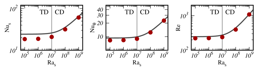
(a) $\mbox{{Pr}}_{s}=10$ and $\mbox{{Ra}}_{\theta}=10^{6}$

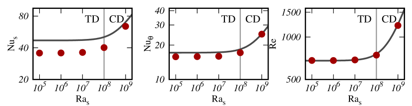
(b) $\mbox{{Pr}}_{s}=10$ and $\mbox{{Ra}}_{\theta}=10^{7}$

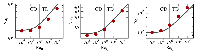
(c) $\mbox{{Pr}}_{s}=10$ and $\mbox{{Ra}}_{s}=10^{7}$

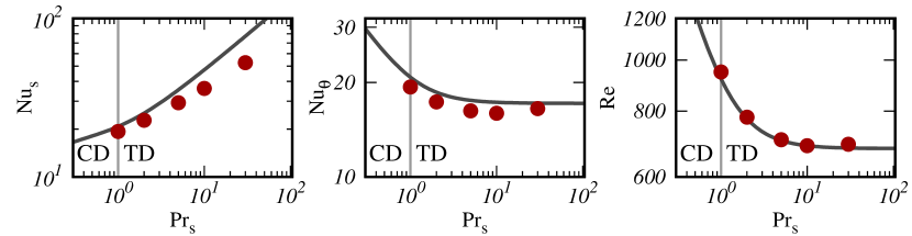
(d) $\mbox{{Ra}}_{\theta}=10^{7}$ and $\mbox{{Ra}}_{s}=10^{7}$

Figure 3: Comparison of the GL theory (lines) to the numerical results (symbols). Each subfigure shows a group of cases listed in table 1. The vertical gray line in every plot indicates the location $\Lambda=1$, which separates the CD and TD regimes.

However, some discrepancy is observed for certain parameters. Among the three global responses, the theoretical prediction for the concentration flux $\mbox{{Nu}}_{s}$ exhibits the biggest deviation from the numerical results, especially in the deep TD regime (with large $\Lambda$). In this regime the flow is mainly driven by the temperature difference, such as the case shown in figures 1e and 1f. All the concentration plumes are very thin and stay in the core regions of the temperature plumes, therefore the buoyancy anomaly associated to concentration and its effects on the momentum field are confined inside the temperature plumes due to the slow sideward diffusion. The morphology and dynamics of such thin concentration plumes are very different from the traditional RB plumes, thus the original scaling arguments of the GL theory become less accurate.

For the opposite situation in the deep CD regime (with small $\Lambda$), although the buoyancy force is mainly generated by the concentration component, the temperature anomaly diffuses faster in the lateral direction and is not confined inside the concentration plumes. The temperature anomaly can directly interact with the momentum field and thus more similar to the situation in the RB flows. Therefore the GL theory performs better in the CD regime than in the TD regime, as shown in figures 3a-c.

IV Conclusions and discussions

In summary, we conducted the direction numerical simulations of the RB convection driven by two scalar components which have different molecular diffusivities. The flow morphology changes for different ratios of the buoyancy forces associated to the two scalar differences. We have generalized the GL theory for the RB convection to the current problem. The results show that the theory captures the overall trends of the dependences of scalar fluxes and flow velocity on the control parameters. For most of the cases the theory predicts the absolute values with good accuracy. This comparison demonstrates the applicability of the GL theory to multiple component convection flows. The accuracy of the theory decreases when the fast-diffusing component dominates the buoyancy force, i.e. in the TD regime. We argue that in this regime, the structures of the slow-diffusing component is very different from those in the traditional RB flows, and the argument in the original GL theory becomes less accurate.

A more refined generalization of the GL theory should assume that the coefficients are not constant but some functions of the density ratio $\Lambda$, and they recover the original GL values when the system degenerates to a single scalar RB flows. The theory also deserves to be tested over a larger parameter space, such as for the scalars with Prandtl number smaller than one, which is of relevance to some astrophysical flows.

References

- Ahlers et al. (2009) Ahlers, G., Grossmann, S. & Lohse, D. 2009 Heat transfer and large scale dynamics in turbulent Rayleigh-Bénard convection. Rev. Mod. Phys. 81, 503–537.
- Bakhuis et al. (2018) Bakhuis, D., Ostilla-Mónico, R., van der Poel, E.P., Verzicco, R. & Lohse, D. 2018 Mixed insulating and conducting thermal boundary conditions in Rayleigh-Bénard convection. J. Fluid Mech. 835, 491–511.
- Chillà & Schumacher (2012) Chillà, F. & Schumacher, J. 2012 New perspectives in turbulent Rayleigh?Bénard convection. Eur. Phys. J. E 35 (7), 58.
- Grossmann & Lohse (2000) Grossmann, S. & Lohse, D. 2000 Scaling in thermal convection: a unifying theory. J. Fluid Mech. 407, 27–56.
- Grossmann & Lohse (2001) Grossmann, S. & Lohse, D. 2001 Thermal convection for large Prandtl numbers. Phys. Rev. Lett. 86 (15), 3316–3319.
- Grossmann & Lohse (2002) Grossmann, S. & Lohse, D. 2002 Prandtl and Rayleigh number dependence of the Reynolds number in turbulent thermal convection. Phys. Rev. E 66 (1), 016305.
- Grossmann & Lohse (2004) Grossmann, S. & Lohse, D. 2004 Fluctuations in turbulent Rayleigh-Bénard convection: The role of plumes. Phys. Fluids 16 (12), 4462–4472.
- Hieronymus & Carpenter (2016) Hieronymus, M. & Carpenter, J.R. 2016 Energy and variance budgets of a diffusive staircase with implications for heat flux scaling. J. Phys. Oceanogr. 46, 2553–2569.
- King et al. (2009) King, E.M., Stellmach, S., Noir, J., Hansen, U. & Aurnou, J. M. 2009 Boundary layer control of rotating convection systems. Nature 457, 301–304.
- Lohse & Xia (2010) Lohse, D. & Xia, K.-Q. 2010 Small-scale properties of turbulent Rayleigh-Bénard convection. Annu. Rev. Fluid Mech. 42, 335–364.
- Ostilla-Mónico et al. (2015) Ostilla-Mónico, R., Yang, Y., van der Poel, E. P., Lohse, D. & Verzicco, R. 2015 A multiple resolutions strategy for direct numerical simulation of scalar turbulence. J. Comput. Phys. 301, 308–321.
- Radko (2013) Radko, T. 2013 Double-diffusive convection. Cambridge, UK: Cambridge University Press.
- Salort et al. (2014) Salort, J., Liot, O., Rusaouen, E., Seychelles, F., Tisserand, J.-C., Creyssels, M., Castaing, B. & Chill , F. 2014 Thermal boundary layer near roughnesses in turbulent Rayleigh-Bénard convection: Flow structure and multistability. Phys. Fluids 26, 015112.
- Shishkina & Wagner (2011) Shishkina, Olga & Wagner, Claus 2011 Modelling the influence of wall roughness on heat transfer in thermal convection. J. Fluid Mech. 686, 568?–582.
- Stevens et al. (2010) Stevens, R.J.A.M., Verzicco, R. & Lohse, D. 2010 Radial boundary layer structure and Nusselt number in Rayleigh-Bénard convection. J. Fluid Mech. 643, 495–507.
- Stevens et al. (2013) Stevens, R. J. A. M., van der Poel, E. P., Grossmann, S. & Lohse, D. 2013 The unifying theory of scaling in thermal convection: the updated prefactors. J. Fluid Mech. 730, 295–308.
- Turner (1985) Turner, J.S 1985 Multicomponent convection. Annu. Rev. Fluid Mech. 17 (1), 11–44.
- Wang et al. (2017) Wang, F., Huang, S.-D. & Xia, K.-Q. 2017 Thermal convection with mixed thermal boundary conditions: effects of insulating lids at the top. J. Fluid Mech. 817, R1.
- Wei et al. (2015) Wei, P., Weiss, S. & Ahlers, G. 2015 Multiple transitions in rotating turbulent Rayleigh-Bénard convection. Phys. Rev. Lett. 114, 114506.
- Xie & Xia (2017) Xie, Y.-C. & Xia, K.-Q. 2017 Turbulent thermal convection over rough plates with varying roughness geometries. J. Fluid Mech. 825, 573–599.
- Yang et al. (2015) Yang, Y., van der Poel, E. P., Ostilla-M ónico, R., Sun, C., Verzicco, R., Grossmann, S. & Lohse, D. 2015 Salinity transfer in bounded double diffusive convection. J. Fluid Mech. 768, 476–491.
- Yang et al. (2016) Yang, Y., Verzicco, R. & Lohse, D. 2016 Scaling laws and flow structures of double diffusive convection in the finger regime. J. Fluid Mech. 802, 667–689.
- Zhu et al. (2017) Zhu, X., Stevens, R.J.A.M., Verzicco, R. & Lohse, D. 2017 Roughness-facilitated local 1/2 scaling does not imply the onset of the ultimate regime of thermal convection. Phys. Rev. Lett. 119, 154501.