New and Improved Algorithms for Unordered Tree Inclusion

Abstract

The tree inclusion problem is, given two node-labeled trees $P$ and $T$ (the “pattern tree” and the “target tree”), to locate every minimal subtree in $T$ (if any) that can be obtained by applying a sequence of node insertion operations to $P$. Although the ordered tree inclusion problem is solvable in polynomial time, the unordered tree inclusion problem is NP-hard. The currently fastest algorithm for the latter is a classic algorithm by Kilpeläinen and Mannila from 1995 that runs in $O(2^{2d}mn)$ time, where $m$ and $n$ are the sizes of the pattern and target trees, respectively, and $d$ is the degree of the pattern tree. Here, we develop a new algorithm that runs in $O(2^{d}mn^{2})$ time, improving the exponential factor from $2^{2d}$ to $2^{d}$ by considering a particular type of ancestor-descendant relationships that is suitable for dynamic programming. We also study restricted variants of the unordered tree inclusion problem.

Keywords: tree inclusion, unordered trees, parameterized algorithms, dynamic programming.

1 Introduction

Tree pattern matching and measuring the similarity of trees are fundamental problem areas in theoretical computer science. One intuitive and previously well-studied measure of the similarity between two rooted, node-labeled trees $T_{1}$ and $T_{2}$ is the tree edit distance, defined as the length of a shortest sequence of node insertion, node deletion, and node relabeling operations that transforms $T_{1}$ into $T_{2}$ [9]. An important special variant of the problem of computing the tree edit distance known as the tree inclusion problem is obtained when the only allowed operations are node insertion operations on $T_{1}$. Here, we assume the following formulation of the problem: given a “pattern tree” $P$ and a “target tree” $T$, locate every minimal subtree in $T$ (if any) that can be obtained by applying a sequence of node insertion operations to $P$. (Equivalently, one may define the tree inclusion problem so that only node deletion operations on $T$ are allowed.) In 1995, Kilpeläinen and Mannila [19] proved that the tree inclusion problem for unordered trees is NP-hard, but solvable in polynomial time when the degree of the pattern tree is bounded from above by a constant. The running time of their algorithm is $O(d\cdot 2^{2d}\cdot mn)=O^{\ast}(2^{2d})=O^{\ast}(4^{d})$, where $m=|P|$, $n=|T|$, and $d$ is the degree of $P$. Throughout this article, the notation “$O^{\ast}(\dots)$” means “$O(\dots)$” multiplied by some function that is a polynomial in $m$ and $n$. E.g., “$O^{\ast}(2^{2d})$” means “$O(2^{2d}\cdot poly(m,n))$”.

Our main contribution is a new algorithm for solving the unordered tree inclusion problem more efficiently. More precisely, its time complexity is $O(d\cdot 2^{d}\cdot mn^{2})=O^{\ast}(2^{d})$, which yields the first improvement in over twenty years. Our bound is obtained by introducing the simple yet useful concept of minimal inclusion and considering a particular type of ancestor-descendant relationships that turns out to be suitable for dynamic programming. Next, we analyze the computational complexity of unordered tree inclusion for some restricted cases; see Table 1 for a summary of the new findings. We give a polynomial-time algorithm for the case where the leaves of $P$ are distinctly labeled and every label appears at most twice in $T$, and an $O^{\ast}(1.619^{d})$-time algorithm for the NP-hard case where the leaves in $P$ are distinctly labeled and each label appears at most three times in $T$. Both of these algorithms effectively utilize some techniques from a polynomial-time algorithm for 2-SAT [8]. (Note that the preliminary version of this paper [5] contained a slower algorithm for the latter case running in $O^{\ast}(1.8^{d})$ time.) Finally, we derive a randomized $O^{\ast}(1.883^{d})$-time algorithm for the case where the heights of $P$ and $T$ are one and two, respectively, via a non-trivial combination of our $O^{\ast}(2^{d})$-time algorithm, Yamamoto’s algorithm for SAT [31], and color-coding [7].

Table 1: The computational complexity of some special cases of the unordered tree inclusion problem. For any tree $T$, $h(T)$ denotes the height of $T$ and $occ(T)$ the maximum number of times that any leaf label occurs in $T$. As indicated in the table, either all nodes or only the leaves are labeled (the former is harder since it generalizes the latter). Note that the fourth case is NP-hard as it generalizes the first two. The algorithm referred to in the last case is randomized.

Restriction	Labels on	Complexity	Result
$h(T)=2$, $h(P)=1$,	all nodes	NP-hard	Corollary 1
$occ(T)=3$, $occ(P)=1$
$h(T)=2$, $h(P)=2$,	leaves	NP-hard	Theorem 2
$occ(T)=3$, $occ(P)=1$
$occ(T)=2$, $occ(P)=1$	all nodes	P	Theorem 3
$occ(T)=3$, $occ(P)=1$	all nodes	$O^{\ast}(1.619^{d})$ time	Theorem 4
$h(T)=2$, $h(P)=1$	all nodes	$O^{\ast}(1.883^{d})$ time	Theorem 5

1.1 Related results

In general, tree edit distance-related problems are computationally harder for unordered trees than for ordered trees. A comprehensive summary of the many results that were already known in 2005 can be found in the survey by Bille [9]. Below, we briefly mention a few of these historical results along with some more recent ones.

When $T_{1}$ and $T_{2}$ are ordered trees, the tree edit distance can be computed in polynomial time. The first algorithm to do so, invented by Tai [28] in 1979, ran in $O(n^{6})$ time, where $n$ is the total number of nodes in $T_{1}$ and $T_{2}$. The time complexity was gradually improved upon until Demaine et al. [15] thirty years later presented an $O(n^{3})$-time algorithm, which was proved to be worst-case optimal under the conjecture that there is no truly subcubic time algorithm for the all-pairs-shortest-paths problem [12]. Pawlik and Augsten [25] developed a robust algorithm whose asymptotic complexity is less than or equal to the complexity of the best competitors for any input instance. In another line of research, since even $O(n^{3})$ time is too slow for similarity search and so-called join operations in XML databases, the focus has been on approximate methods. Garofalakis and Kumar [17] gave an algorithm for embedding the tree edit distance in a high-dimensional $L_{1}$-norm space with a guaranteed distortion, and recently, Boroujen et al. provided an $O(n^{2})$-time $(1+\varepsilon)$-approximation algorithm [11].

In contrast, the tree edit distance problem is NP-hard for unordered trees [34]. It is MAX SNP-hard even for binary trees in the unordered case [33], which implies that it is unlikely to admit a polynomial-time approximation scheme. Some exponential-time algorithms for this problem variant were developed by Akutsu et al. [3, 6]. As for parameterized algorithms, Shasha et al. [27] gave an $O(4^{\ell_{1}+\ell_{2}}\cdot\min(\ell_{1},\ell_{2})\cdot mn)$-time algorithm for the problem, where $\ell_{1}$ and $\ell_{2}$ are the numbers of leaves in $T_{1}$ and $T_{2}$, respectively. Taking the tree edit distance (denoted by $k$) to be the parameter instead, an $O^{\ast}(2.62^{k})$-time algorithm for the unit-cost edit operation model was developed by Akutsu et al. [4].

As mentioned above, Kilpeläinen and Mannila [19] proved that the unordered tree inclusion problem is NP-hard and gave an algorithm that runs in $O(d\cdot 2^{2d}\cdot mn)$ time, where $m=|P|$, $n=|T|$, and $d$ is the degree of $P$. Bille and Gørtz [10] presented a fast algorithm for the case of ordered trees, and Valiente [30] gave a polynomial-time algorithm for a constrained version of the unordered case. Piernik and Morzy [26] introduced a similar problem for ordered trees and developed an efficient algorithm. Finally, we remark that the special case of the tree inclusion problem in which node insertion operations are only allowed to insert new leaves corresponds to a subtree isomorphism problem, which can be solved in polynomial time even for unordered trees [23].

1.2 Applications

Research in tree pattern matching has led to algorithms used in numerous practical applications over the years. Some examples include fast methods for querying structured text databases, document similarity search, natural language processing, compiler optimization, automated theorem proving, comparison of RNA secondary structures, assessing the accuracy of phylogenetic tree reconstruction methods, and medical image analysis [10, 14, 19, 30]. Recently, due to the rapid advance of AI technology, matching methods for knowledge bases have become increasingly important. In particular, researchers in the database community have enhanced the basic subtree similarity search technique to search a knowledge base of hierarchically structured information under various definitions of similarity; e.g., Cohen and Or [14] presented a general subtree similarity search algorithm that is compatible with a wide range of tree distance functions, and Chang et al. [13] proposed a top-$k$ tree matching algorithm. In the Natural Language Processing (NLP) field, researchers are applying deep learning techniques to NLP problems and developing algorithms for processing parsing/dependency trees [22].

As an example of the versatility of tree comparison algorithms, three different tree pattern matching applications involving glycan data from the KEGG database [18], weblogs data [32], and bibliographical data from ACM, DBLP, and Google Scholar [21] were all expressed in terms of an optimization version of the unordered tree inclusion problem named the extended tree inclusion problem and studied experimentally by Mori et al. [24]. Note that for bibliographic matching, a single article usually has at most two or three versions (e.g., preprint, conference version, and journal version), and it is very rare that a single article includes two co-authors with exactly the same family and given names. Therefore, two reasonable assumptions when modeling bibliographic matching as the tree inclusion problem are that the leaves of the pattern tree $P$ are distinctly labeled and that each label occurs at most $c$ times in the target tree $T$ for some bounded value of $c$.

Another important restriction is on the height of trees. In entity resolution, some authors have applied tree matching where entities are usually represented by a shallow tree. Mori et al. [24] represented a bibliographic record by a tree of height 2 and linked identical records in two different bibliographic databases. Konda et al. [20] evaluated their entity resolution system by using various datasets. Movie records from IMDb used in their experiment, for example, were extracted from IMDb web pages in HTML format. The fields of the movie record are included in a subtree of height 7 in the web page. Since the HTML code contains many tags for rendering the page, the height of trees required for the movie record is much lower. Apart from these practical viewpoints, it is of theoretical interests to study restricted cases because the unordered tree inclusion problem remains NP-hard even in considerably restricted cases, as shown in Table 1.

2 Definitions and notation

From here on, all trees are assumed to be rooted, unordered, and node-labeled. Let $T$ be a tree. We use $r(T)$, $h(T)$, and $V(T)$ to denote the root of $T$, the height of $T$, and the set of nodes in $T$, respectively. For any $v\in V(T)$, $\ell(v)$ is the node label of $v$ and $Chd(v)$ is the set of children of $v$. Furthermore, $Anc(v)$ and $Des(v)$ are the sets of strict ancestors and strict descendants of $v$, respectively (i.e., $v$ itself is excluded from these sets), whereas $AncDes(v)=Anc(v)\cup Des(v)\cup\{v\}$ is the set of all ancestors of $v$, all descendants of $v$, and $v$. Also, $T(v)$ denotes the subtree of $T$ induced by $Des(v)\cup\{v\}$.

A node insertion operation on a tree $T$ is an operation that creates a new node $v$ having any label and then: (i) attaches $v$ as a child of some node $u$ currently in $T$ and makes $v$ become the parent of a (possibly empty) subset of the children of $u$ instead of $u$, so that $u$ is no longer their parent; or (ii) makes the current root of $T$ become a child of $v$ and lets $v$ become the root of $T$ instead. For any two trees $T_{1}$ and $T_{2}$, we say that $T_{1}$ is included in $T_{2}$ if there exists a sequence of node insertion operations that, when applied to $T_{1}$, yields $T_{2}$. Equivalently, $T_{1}$ is included in $T_{2}$ if $T_{1}$ can be obtained by applying a sequence of node deletion operations (defined as the inverse of a node insertion operation) to $T_{2}$.

A mapping between two trees $T_{1}$ and $T_{2}$ is a subset $M\subseteq V(T_{1})\times V(T_{2})$ such that for every $(u_{1},v_{1}),(u_{2},v_{2})\in M$, it holds that: (i) $u_{1}=u_{2}$ if and only if $v_{1}=v_{2}$; and (ii) $u_{1}$ is an ancestor of $u_{2}$ if and only if $v_{1}$ is an ancestor of $v_{2}$. Condition (i) states that each node appears at most once in $M$, and condition (ii) states that ancestor-descendant relations must be preserved. A mapping $M$ between $T_{1}$ and $T_{2}$ such that $|M|=|V(T_{1})|$ and $u$ and $v$ have the same node label for every $(u,v)\in M$ is called an inclusion mapping (see Fig. 1 for an example). It is known that $T_{1}$ is included in $T_{2}$ if and only if there exists an inclusion mapping between $T_{1}$ and $T_{2}$ [28]. We write $T_{1}(u)\subset T_{2}(v)$ if $T_{1}(u)$ is included in $T_{2}(v)$ under the additional condition that there exists an inclusion mapping that maps $u$ to $v$. For any two trees $T_{1}$ and $T_{2}$, $T_{1}\sim T_{2}$ means that $T_{1}$ is isomorphic to $T_{2}$, in the sense that node labels have to be preserved.

In the tree inclusion problem, the input is two trees $P$ and $T$, also referred to as the “pattern tree” and the “target tree”, and the objective is to locate every minimal subtree of $T$ that includes $P$, where $T(v)$ is called a minimal subtree if it minimally includes $P$, the definition of which is given below. For any instance of the tree inclusion problem, we define $m=|V(P)|$ and $n=|V(T)|$, and let $d$ denote the degree of $P$, i.e., the maximum number of children of any node in $P$. We assume w.l.o.g. (without loss of generality) that $m\leq n$ because otherwise $P$ cannot be included in $T$. The following concept plays a key role in our algorithm (see Fig. 1 for an illustration).

Definition 1.

For any instance of the tree inclusion problem and any $u\in V(P)$ and $v\in V(T)$, $T(v)$ is said to minimally include $P(u)$ (written as $P(u)\prec T(v)$) if $P(u)\subset T(v)$ holds and there is no $v^{\prime}\in Des(v)$ such that $P(u)\subset T(v^{\prime})$.

We may simply use $P$ and $T$ in place of $P(u)$ and $T(v)$ if $u$ and $v$ are the roots of $P$ and $T$, respectively. Locating every minimal subtree is reasonable because $P(u)\subset T(v^{\prime})$ holds for all ancestors $v^{\prime}$ of $v$ if $P(u)\prec T(v)$ holds.

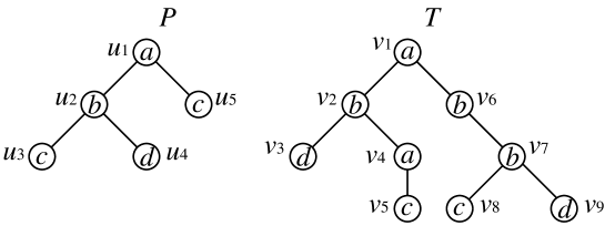
Figure 1: An example of unordered tree inclusion. Here, $P\subset T$ holds by an inclusion mapping $M=\{(u_{1},v_{1}),(u_{2},v_{2}),(u_{3},v_{5}),(u_{4},v_{3}),(u_{5},v_{8})\}$. $P(u_{2})\subset T(v_{2})$, $P(u_{2})\subset T(v_{6})$, and $P(u_{2})\subset T(v_{7})$ hold as well. Furthermore, $P\prec T$, $P(u_{2})\prec T(v_{2})$, and $P(u_{2})\prec T(v_{7})$ hold, but $P(u_{2})\prec T(v_{6})$ does not hold.

Proposition 1.

Given any instance of the tree inclusion problem and any $u\in V(P)$ and $v\in V(T)$ with $Chd(u)=\{u_{1},\ldots,u_{d}\}$, it holds that $P(u)\subset T(v)$ if and only if the following conditions are satisfied:

• $\ell(u)=\ell(v)$;

• $v$ has a set of descendants $D(v)=\{v_{1},\ldots,v_{d}\}$ such that $v_{i}\notin Des(v_{j})$ for every $i\neq j$; and

• there exists a bijection $\phi$ from $Chd(u)$ to $D(v)$ such that $P(u_{i})\prec T(v_{i})$ holds for every $i\in\{1,2,\ldots,d\}$.

Proof.

Suppose that Conditions (1)-(3) are satisfied. Condition (3) implies that there exists an injection mapping $\phi^{\prime}$ between the forest induced by $u_{1},\ldots,u_{d}$ and their descendants and the forest induced by $v_{1},\ldots,v_{d}$ and their descendants such that $\phi^{\prime}(u_{i})=v_{i}$. Let $\phi^{\prime\prime}=\phi^{\prime}\cup\{(u,v)\}$. Since $u_{1},\ldots,u_{d}$ are the children of $u$ and $v_{1},\ldots,v_{d}$ are descendants of $v$, $\phi^{\prime\prime}$ is an inclusion mapping and thus $P(u)\subset T(v)$ holds.

Conversely, suppose that $P(u)\subset T(v)$ holds, which means that there exists an inclusion mapping $\phi$ from $P(u)$ to $T(v)$ with $\phi(u)=v$. Let $w_{i}=\phi(u_{i})$ for $i=1,\ldots,d$. Then, $w_{i}\notin Des(w_{j})$ holds for every $i\neq j$ because $\phi$ is an inclusion mapping. Furthermore, for each $w_{i}$, there must exist $v_{i}\in\{w_{i}\}\cup Des(w_{i})$ such that $P(u_{i})\prec T(v_{i})$ holds with an inclusion mapping $\phi_{i}$ from $P(u_{i})$ to $T(v_{i})$ satisfying $\phi_{i}(u_{i})=v_{i}$. Note that $v_{i}\notin Des(v_{j})$ holds for every $i\neq j$ because $w_{i}\notin Des(w_{j})$ holds for every $i\neq j$. Let $\phi^{\prime}=\{(u,v)\}\cup\phi_{1}\cup\ldots\phi_{d}$. Condition (1) is satisfied because $(u,v)\in\phi^{\prime}$. Here we let $D(v)=\{v_{1},\ldots,v_{d}\}$. Then, Condition (2) is satisfied as stated above. Condition (3) is also satisfied because $\phi^{\prime}(u_{i})=v_{i}$ holds for all $i=1,\ldots,d$. ∎

Proposition 1 essentially states that the children of $u$ must be mapped to descendants of $v$ that do not have ancestor-descendant relationships. Since $P$ is included in $T$ if and only if there exists a $v\in V(T)$ with $P\prec T(v)$, we need to determine if $P(u)\prec T(v)$, assuming that whether $P(u_{j})\prec T(v_{i})$ holds is known for all $(u_{j},v_{i})$ with $u_{j}\in Des(u)\cup\{u\}$, $v_{i}\in Des(v)\cup\{v\}$, and $(u_{j},v_{i})\neq(u,v)$. This assumption is satisfied if we apply a dynamic programming procedure to determine if $P\prec T(v)$, using an $O(mn)$ size table and following any partial ordering on $(u,v)$s in $V(P)\times V(T)$ such that $(u,v)$ precedes $(u^{\prime},v^{\prime})$ if and only if $u^{\prime}\in Des(u)\cup\{u\}$, $v^{\prime}\in Des(v)\cup\{v\}$, and $(u^{\prime},v^{\prime})\neq(u,v)$.

Proposition 2.

Suppose that $P(u)\prec T(v)$ can be determined in $O(f(d,m,n))$ time, assuming that whether $P(u_{j})\prec T(v_{i})$ holds is known for all pairs $(u_{j},v_{i})$ such that $(u_{j},v_{i})\in V(P(u))\times V(T(v))\setminus\{(u,v)\}$. Then the unordered tree inclusion problem can be solved in $O(f(d,m,n)\cdot mn)$ time by using a bottom-up dynamic programming procedure.

3 An $O(d\cdot 2^{d}\cdot mn^{2})$-time algorithm

The core of Kilpeläinen and Mannila’s algorithm [19] for unordered tree inclusion is the computation of a set $S(v)$ for each node $v\in V(T)$, also called the match system for target node $v$. In their paper, $S(v)$ was originally defined as a set of subsets of nodes from $P$, where each such subset consists of the root nodes in a subforest of $P$ that is included in $T(v)$. However, $S(v)$ was restricted to subsets of $Chd(u)$ for a single node $u$ in $P$ when the bounded outdegree case was considered. We employ this restricted definition in this paper and define $S(v)$ for any fixed $u\in V(P)$ by:

$$S(v) = \{U\subseteq Chd(u)\,|\,P(U)\subset T(v)\},$$

where $P(U)$ is the forest induced by the nodes in $U$ and their descendants and $P(U)\subset T(v)$ means that every tree from $P(U)$ is included in $T(v)$ without overlap (i.e., $T(v)$ can be obtained from $P(U)$ by node insertion operations). For details, see [19].

Kilpeläinen and Mannila’s algorithm [19] computes the $S(v)$-sets in a bottom-up order. It fixes an arbitrary left-to-right ordering of the nodes of $T$ (the ordering will not affect the correctness). Precisely, the left-to-right ordering is determined as follows. We assume that for each node having two or more children, a left-to-right ordering is given to the children. For any two nodes $v_{i},v_{j}\in V(T)$ (resp., $v_{i},v_{j}\in V(P)$) that do not have any ancestor-descendant relationship, let $v$ be the lowest common ancestor, which is uniquely determined. For any descendant $v_{k}$ of $v$, let $v_{k}^{\prime}$ be the child of $v$ such that $v_{k}$ is a descendant of $v_{k}^{\prime}$ or $v_{k}=v_{k}^{\prime}$. Then, $v_{i}$ is left (resp., right) of $v_{j}$ if and only if $v_{i}^{\prime}$ is a left (resp., right) sibling of $v_{j}^{\prime}$. Note that left-right relationships are defined for nodes only if they do not have any ancestor-descendant relationship. Below, we denote “$v_{i}$ is left of $v_{j}$” by $v_{i}\triangleleft v_{j}$. To compute $S(v)$, their algorithm performs the following operation from left to right for the children $v_{1},\ldots,v_{l}$ of $v$:

$$S := \{A\cup B\,|\,A\in S,\,B\in S(v_{i})\},$$

starting with $S=\emptyset$, and then $S(v)$ is assigned the resulting $S$. Clearly, the size of $S(v)$ is no greater than $2^{d}$. However, this way of updating $S$ causes an $\Omega(2^{2d})$-factor in the running time because it examines $\Omega(2^{d})\times\Omega(2^{d})$ set pairs. To avoid this bottleneck, we need a new approach for computing $S(v)$, explained next. We shall focus on how to determine if $P(u)\prec T(v)$ holds for a fixed $(u,v)$ because this part is crucial for reducing the time complexity.

Assume w.l.o.g. that $u$ has $d$ children and write $Chd(u)=\{u_{1},\ldots,u_{d}\}$. To simplify the presentation, we will assume until the end of this section that $P(u_{i})\sim P(u_{j})$ does not hold for any $u_{i},u_{j}\in Chd(u)$ with $u_{i}\neq u_{j}$. For any $v_{i}\in V(T(v))$, define $M(v_{i})$ by:

$$M(v_{i}) = \{u_{j}\in Chd(u)\,|\,P(u_{j})\prec T(v_{i})\}.$$

For example, $M(v_{0})=\emptyset$, $M(v_{2})=\{u_{C}\}$, and $M(v_{3})=\{u_{D},u_{E}\}$ in Fig. 2. Note that $M(v_{i})$ is known for all descendants $v_{i}$ of $v$ before testing $P(u)\prec T(v)$ and does not change during the course of this testing. For any $v_{i}\in V(T(v))$, $LF(v,v_{i})$ denotes the set of nodes in $V(T(v))$ each of which is left of $v_{i}$ (see Fig. 2 for an example). Next, define $S(v,v_{i})$ by:

$$S(v,v_{i}) = \{U\subseteq Chd(u)\,|\,P(U)\subset T(LF(v,v_{i}))\}\cup$$

$$\{U\subseteq Chd(u)\,|\,(U=U^{\prime}\cup\{u_{j}\})\land(P(U^{\prime})\subset T(LF(v,v_{i})))\land$$

$$~{}~{}~{}~{}~{}~{}~{}~{}~{}~{}~{}~{}~{}~{}~{}~{}~{}~{}~{}~{}~{}~{}~{}~{}~{}~{}~{}~{}~{}~{}~{}~{}~{}~{}~{}~{}~{}~{}~{}~{}~{}~{}~{}~{}~{}(u_{j}\in M(v_{i}))\}$$

where $T(LF(v,v_{i}))$ is the forest induced by the nodes in $LF(v,v_{i})$ and their descendants. Note that $P(\emptyset)\subset T(...)$ always holds. Note also that each element of $S(v,v_{i})$ is a subset of the children of $u$ that are included in the forest induced by the nodes left to $v_{i}$ and in $V(T(v_{i}))$ under the condition that there exists at most one child $u_{j}$ such that $P(u_{j})$ is included in $T(v_{i})$ in the corresponding inclusion mapping. The motivation for introducing $S(v,v_{i})$ is that Lemma 1 below will allow us to recover $S(v)$ from a collection of $S(v,v_{i})$-sets, and the $S(v,v_{i})$-sets can be computed efficiently with dynamic programming. We explain $S(v,v_{i})$ using an example based on Fig. 2. Suppose we have the relations $P(u_{A})\prec T(v_{1})$, $P(u_{B})\prec T(v_{1})$, $P(u_{C})\prec T(v_{2})$, $P(u_{D})\prec T(v_{3})$, $P(u_{E})\prec T(v_{3})$, $P(u_{D})\prec T(v_{4})$, and $P(u_{F})\prec T(v_{4})$. Then, the following holds:

$S(v,v_{0})=\{~{}\emptyset~{}\}$,

$S(v,v_{1})=\{~{}\emptyset,~{}\{u_{A}\},~{}\{u_{B}\}~{}\}$,

$S(v,v_{2})=\{~{}\emptyset,~{}\{u_{C}\}~{}\}$,

$S(v,v_{3})=\{~{}\emptyset,~{}\{u_{D}\},~{}\{u_{E}\}~{}\}$,

$S(v,v_{4})=\{~{}\emptyset,~{}\{u_{D}\},~{}\{u_{E}\},~{}\{v_{F}\},~{}\{u_{D},u_{E}\},~{}\{u_{D},u_{F}\},~{}\{u_{E},u_{F}\}~{}\}$.

Figure 2: An example. A triangle $X$ attached to $v_{i}$ means that $P(u_{X})\subset T(v_{i})$. Note that the triangle $D$ appears at $v_{2}$, $v_{3}$, and $v_{4}$. However, $P(u_{D})\prec T(v_{2})$ does not hold since it does not satisfy the minimality condition. Therefore, $u_{D}$ may be matched to $v_{3}$ or $v_{4}$, but $u_{D}$ will never be matched to $v_{2}$ in TreeIncl1.

Next, we present a dynamic programming-based algorithm named TreeIncl1, for determining if $P(u)\prec T(v)$. To compute all the $S(v,v_{i})$-sets, we construct a DAG (directed acyclic graph) $G(V,E)$ from $T(v)$, as illustrated in Fig. 3. Here, $V$ is defined by $V=V(T(v))-\{v\}$, and $E$ is defined by $E=\{(v_{i},v_{j})\,|\,v_{i}\triangleleft v_{j}\}$. We define $Pred(v_{i})$ by $Pred(v_{i})=\{v_{j}\,|\,(v_{j},v_{i})\in E\}$, meaning the set of the “predecessors” of $v_{i}$, and also being equivalent to $LF(v,v_{i})$. TreeIncl1 traverses $G(V,E)$ so that node $v_{i}$ is visited only after all of its predecessors have been visited, at which point it runs the procedure ComputeSet$(v,v_{i})$ below to compute and store $S(v,v_{i})$ for this $v_{i}$. Recall that $M(v_{i})=\{u_{j}\in Chd(u)\,|\,P(u_{j})\prec T(v_{i})\}$.

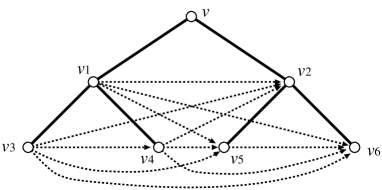
Figure 3: Example of the DAG $G(V,E)$ constructed from $T(v)$, where $v\notin V$, $E$ is shown by dotted arrows, and $T(v)$ is shown by bold lines.

Procedure ComputeSet$(v,v_{i})$:

• If $Pred(v_{i})=\emptyset$ then $S(v,v_{i}):=\{\emptyset\}\cup\{\{u_{h}\}\,|\,u_{h}\in M(v_{i})\}$

• Else:

• $S_{0}(v_{i}):=\bigcup_{v_{j}\in Pred(v_{i})}S(v,v_{j})$

• $S(v,v_{i}):=S_{0}(v_{i})\cup\{S\cup\{u_{h}\}\,|\,u_{h}\in M(v_{i}),S\in S_{0}(v_{i})\}$

Finally, after $G(V,E)$ has been completely traversed, TreeIncl1 assigns $S(v):=\bigcup_{v_{i}\in Des(v)}S(v,v_{i})$. Then $P(u)$ is included in $T(v)$ with $u$ corresponding to $v$ if and only if $u$ and $v$ have the same label and $Chd(u)\in S(v)$. Note that $S(v)=\emptyset$ holds for each $v$ if $Chd(u)=\emptyset$.

Lemma 1.

Procedure ComputeSet$(v,v_{i})$ correctly computes $S(v,v_{i})$s, and $S(v)=\cup_{v_{i}\in Des(v)}S(v,v_{i})$.

Proof.

First we show that ComputeSet$(v,v_{i})$ correctly computes $S(v,v_{i})$s. It is seen from Proposition 1 that $U\in S(v,v_{i})$ holds for $U=\{u_{i_{1}},\ldots,u_{i_{k}}\}\subseteq Chd(u)$ ($U=\emptyset$ if $k=0$) if and only if there exists a sequence of nodes $(v_{j_{1}},v_{j_{2}},\ldots,v_{j_{k}})$ such that $P(u_{i_{p}})\prec T(v_{j_{p}})$ holds for all $p=1,\ldots,k$ and $v_{j_{1}}\triangleleft v_{j_{2}}\triangleleft\cdots\triangleleft v_{j_{k}}$ (by appropriately renumbering indices of $u_{i_{1}},\ldots,u_{i_{k}}$), where $v_{j_{k}}=v_{i}$ or $v_{j_{k}}\triangleleft v_{i}$. On the other hand, it is seen from ComputeSet$(v,v_{i})$ that this procedure examines all possible sequences such that $v_{j_{1}}\triangleleft v_{j_{2}}\triangleleft\cdots\triangleleft v_{j_{k^{\prime}}}$ with $v_{j_{k^{\prime}}}=v_{i}$ or $v_{j_{k^{\prime}}}\triangleleft v_{i}$, and adds at most one $u_{h}\in M(v_{j_{p}})$ to each set in $S_{0}(v_{j_{p}})$. It is also seen that the procedure and the above discussion that $S_{0}(v_{j_{p}})$ consists of $U$s such that $U\subseteq Chd(u)$ and $P(U)\subset T(LF(v,v_{j_{p}}))$. Therefore, we can see from the definition of $M(\ldots)$ that ComputeSet$(v,v_{i})$ correctly computes $S(v,v_{i})$s.

Then we show the second statement of the lemma. Let $U\in S(v)$ and $d_{U}=|U|$. Let $\phi$ be an injection from $U$ to $Des(v)$ giving an inclusion mapping for $P(U)\subset T(v)$, which is the one guaranteed by Proposition 1. Let $\{v_{1}^{\prime},\ldots,v_{d_{U}}^{\prime}\}=\{\phi(u_{j})|u_{j}\in U\}$, where $v_{1}^{\prime}\triangleleft v_{2}^{\prime}\triangleleft\cdots\triangleleft v_{d_{U}}^{\prime}$. Then, $v_{i}^{\prime}\in LF(v,v_{i+1}^{\prime})$ and $v_{i}^{\prime}\in LF(v,v_{d_{U}}^{\prime})$ hold for all $i=1,\ldots,d_{U}-1$. Furthermore, $P(u_{j})\prec T(v_{i}^{\prime})$ holds for $v_{i}^{\prime}=\phi(u_{j})$. Therefore, $U\in S(v,v_{d_{U}}^{\prime})$.

It is straightforward to see that $S(v,v_{i})$ does not contain any element not in $S(v)$. ∎

The overall procedure of TreeIncl1is given by the pseudocode of Algorithm 1. In this procedure, we traverse nodes in both $P$ and $T$ from left to right n the postorder (i.e., leaves to the root). We maintain $Min(u)$ for $u\in V(P)$ (resp., $Min(v)$ for $v\in V(T)$) that consists of the currently available nodes $v^{\prime}$ (resp., $u^{\prime}$) such that $P(u)\prec T(v^{\prime})$ (resp., $P(u^{\prime})\prec T(v)$).

Algorithm 1 TreeIncl1$(P,T)$

  for all $v\in V(P)\cup V(T)$ do

     $Min(v):=\emptyset$

  end for

  for all $u\in V(P)$ in postorder do

     for all $v\in V(T)$ in postorder do

        $M(v):=\{u_{j}\in Chd(u)|u_{j}\in Min(v)\}$

        for all $v_{i}\in Des(v)$ in postorder do

           ComputeSet$(v.v_{i})$

        end for

        $S(v):=\cup_{v_{i}\in Des(v)}S(v,v_{i})$

        if $Chd(u)\in S(v)$ and $u\notin Min(v_{i})$ for all $v_{i}\in Des(v)$ and $\ell(u)=\ell(v)$ then

           $Min(v):=Min(v)\cup\{u\}$

           $Min(u):=Min(u)\cup\{v\}$

        end if

     end for

  end for

  return  $Min(r(P))$

Lemma 2.

TreeIncl1 outputs the set of all nodes $v$ such that $P\prec T(v)$ in $O(d\cdot 2^{d}\cdot mn^{3})$ time using $O(d\cdot 2^{d}\cdot n+mn)$ space.

Proof.

Since the correctness follows from Lemma 1, we analyze the time complexity.

The sizes of the $S(v)$, $S(v,v_{i_{j}})$s, and $S_{0}(v_{i})$s are $O(d\cdot 2^{d})$, where we can use a simple bit vector of size $O(d)$ to represent each subset of $U$. The computation of each of these sets takes $O(d\cdot 2^{d}\cdot n)$ time. Since the number of $S(v,v_{i_{j}})$s and $S_{0}(v_{i})$s per $(u,v)\in V(P)\times V(T)$ are $O(n)$, the total computation time for $S(v,v_{i_{j}})$s per $(u,v)$ is $O(d\cdot 2^{d}\cdot n^{2})$. Hence, the total computation time for computing $S(v)$s for all $(u,v)$s is $O(d\cdot 2^{d}\cdot mn^{3})$.

Since the size of each $S(v,v_{i})$ is $O(d\cdot 2^{d})$ and we need to maintain $S(v,v_{i})$ for $v_{i}\in Des(v)$ per $(u,v)$, $O(d\cdot 2^{d}\cdot n)$ space is enough to maintain $S(v,v_{i})$s. Note that we can re-use the same space for different $(u.v)$s.

The time needed for other operations can be analyzed as follows. We can use simple bit vectors to maintain $Min(u)$s and $Min(v)$s, which need $O(mn)$ space in total and $O(1)$ time per addition of an element or checking of the membership. Therefore, the total computation time required to maintain $Min(u)$s and $Min(v)$s is $O(mn)$. Furthermore, $M(v)$ can be computed in $O(d)$ time per $(u,v)$ and thus the total time to compute $M(v)$s is $O(dmn)$, and “$u\notin Min(v_{i})$ for all $v_{i}\in Des(v)$” can be checked in $O(|Des(v)|)\leq O(n)$ time per $(u,v)$ and thus the total computation time needed for this checking is $O(mn^{2})$.

Therefore, the time and space complexities of TreeIncl1 are $O(d\cdot 2^{d}\cdot mn^{3})$ and $O(d\cdot 2^{d}\cdot n+mn)$, respectively. ∎

Remark: If there exist $u_{i},u_{j}\in Chd(u),u_{i}\neq u_{j}$ such that $P(u_{i})\sim P(u_{j})$, we treat each element in $S(v)$, $S(v,v_{i_{j}})$s, and $S_{0}(v_{i})$s as a multiset where any $u_{i}$ and $u_{j}$ such that $P(u_{i})\sim P(u_{j})$ are identified and the multiplicity of $u_{i}$ is bounded by the number of $P(u_{j})$s isomorphic to $P(u_{i})$. Then, since $|Chd(u)|\leq d$ for all $u$ in $P$, the size of each multiset is at most $d$ and the number of different multisets is not greater than $2^{d}$. Therefore, the same time complexity result holds. (The same arguments can be applied to the following sections.) Note that by treating $u_{i}$ and $u_{j}$ separately, we do not need to modify the algorithm.

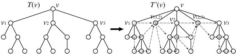
Figure 4: Example of $T^{\prime}(v)$ and $G^{\prime}(V^{\prime},E^{\prime})$. $E^{\prime}$ is shown by dashed arrows.

Next, we discuss how to improve the efficiency of TreeIncl1. Actually, to compute $S_{0}(v_{i})$, it is not necessary to consider all of the $v_{i_{j}}$s that are left of $v_{i}$. Instead, we can construct a tree $T^{\prime}(v)$ from a given $T(v)$ according to the following rule (see Fig. 4 for an illustration):

• For each pair of consecutive siblings $(v_{i},v_{j})$ in $T(v)$, add a new sibling (leaf) $v_{(i,j)}$ between $v_{i}$ and $v_{j}$.

Newly added nodes are called virtual nodes. All virtual nodes have the same label that does not appear in $P$, to ensure that no $u\in V(P)$ is in $M(v_{(i,j)})$. We then construct a DAG $G^{\prime}(V^{\prime},E^{\prime})$ on $V^{\prime}=V(T^{\prime}(v))$ where $(v_{i},v_{j})\in E^{\prime}$ if and only if one of the following holds:

• $v_{j}$ is a virtual node, and $v_{i}$ is in the rightmost path of $T^{\prime}(v_{j_{1}})$, where $v_{j}=v_{(j_{1},j_{2})}$; or

• $v_{i}$ is a virtual node, and $v_{j}$ is in the leftmost path of $T^{\prime}(v_{i_{2}})$, where $v_{i}=v_{(i_{1},i_{2})}$.

By replacing $G(V,E)$ by $G^{\prime}(V^{\prime},E^{\prime})$ in TreeIncl1 (and keeping all other steps intact), we obtain what we call TreeIncl2. Note that in TreeIncl2, $v_{(i,j)}$s are treated in the same ways as for $v_{i}$s and thus we need not introduce the definitions for such terms as $S(v.v_{(i,j)})$ and $LF(v,v_{(i,j)})$ nor change the definition of $S(v.v_{i})$.

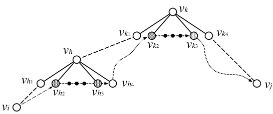
Figure 5: Illustration of a path from $v_{i}$ to $v_{j}$ in the proof of Lemma 3.

Lemma 3.

TreeIncl2 computes $S(v,v_{i})$s for all $v_{i}\in Des(v)$ in $O(d\cdot 2^{d}\cdot n)$ time per $(u,v)\in V(P)\times V(T)$.

Proof.

First we prove that there exists a path in $G^{\prime}(V^{\prime},E^{\prime})$ from $v_{i}\in V$ to $v_{j}\in V$ if and only if $v_{i}\triangleleft v_{j}$ (see also Fig. 5). It can be seen from the definition of the left-right relationship that if $(v_{i},v_{k})\in E^{\prime}$ and $(v_{k},v_{j})\in E^{\prime}$ where $v_{i},v_{j}\in V$ and $v_{k}$ is a virtual node, then $v_{i}\triangleleft v_{j}$. Since virtual nodes and non-virtual nodes appear alternatively in every path in $G^{\prime}(V^{\prime},E^{\prime})$, the “only if” part holds. Suppose that $v_{i}\triangleleft v_{j}$ holds for $v_{i},v_{j}\in V$. Let $v_{k}$ be the lowest common ancestor of $v_{i}$ and $v_{j}$. We assume w.l.o.g. that $v_{i}$ or $v_{j}$ is not a child of $v_{k}$ because the other cases can be proved in the same way. Let $v_{k_{1}},v_{k_{2}},v_{k_{3}},v_{k_{4}}$ be children of $v_{k}$ such that $v_{k_{1}}\in Anc(v_{i})$, $(v_{k_{1}},v_{k_{2}})\in E^{\prime}$, $(v_{k_{3}},v_{k_{4}})\in E^{\prime}$, and $v_{k_{4}}\in Anc(v_{j})$, where $v_{k_{2}}$ and $v_{k_{3}}$ are virtual nodes and can be the same node. We show that there exists a path in $G^{\prime}(V^{\prime},E^{\prime})$ from $v_{i}$ to $v_{k_{2}}$. Let $v_{h}$ be the lowest ancestor of $v_{i}$ that has children $v_{h_{1}},v_{h_{2}},v_{h_{3}},v_{h_{4}}$ such that $v_{h_{1}}\in Ans(v_{i})$, $(v_{h_{1}},v_{h_{2}})\in E^{\prime}$, $(v_{h_{3}},v_{h_{4}})\in E^{\prime}$, and $v_{h_{4}}$ ($\neq v_{h_{1}}$) is the rightmost child of $v_{h}$, where $v_{h_{2}}$ and $v_{h_{3}}$ are virtual nodes and can be the same node. Then, $(v_{i},v_{h_{2}})\in E^{\prime}$ holds from the construction of $G^{\prime}(V^{\prime},E^{\prime})$ and thus there exists a path from $v_{i}$ to $v_{h_{4}}$. We can repeat this procedure by regarding $v_{h_{4}}$ as $v_{i}$, and so on, from which it follows that there exists a path in $G^{\prime}(V^{\prime},E^{\prime})$ from $v_{i}$ to $v_{k_{2}}$. It is also seen from the symmetry on the left-right relationship that there exists a path in $G^{\prime}(V^{\prime},E^{\prime})$ from $v_{k_{3}}$ to $v_{j}$. Furthermore, there clearly exists a path in $G^{\prime}(V^{\prime},E^{\prime})$ from $v_{k_{2}}$ to $v_{k_{3}}$, which completes the proof of the “if” part.

Moreover, from the above discussion, it can be seen that TreeIncl2 examines the same set of sequences $v_{j_{1}}\triangleleft v_{j_{2}}\triangleleft\cdots\triangleleft v_{j_{k^{\prime}}}$ as TreeIncl1 examines when ignoring virtual nodes. Furthermore, addition of an element is not performed at any virtual node, and no element is deleted at any virtual or non-virtual node $v$ in constructing $S(v)$. Therefore, TreeIncl2 correctly computes $S(v,v_{i})$s.

Next we analyze the time complexity. We can see that $|E^{\prime}|=O(n)$ since:

• $|V(T^{\prime}(v))|=O(n)$;

• each non-virtual node in $G^{\prime}(V^{\prime},E^{\prime})$ has at most one incoming edge and at most one outgoing edge; and

• each new edge connects a non-virtual node and virtual node.

Therefore, the total number of set operations is $O(d\cdot 2^{d}\cdot n)$, and the lemma follows. ∎

From Lemmas 2 and 3, we have the following main theorem.

Theorem 1.

Unordered tree inclusion can be solved in $O(d\cdot 2^{d}\cdot mn^{2})$ time and $O(d\cdot 2^{d}\cdot n+mn)$ space.

If we use the height $h(T)$ of a tree $T$ as an additional parameter, we can express the time complexity as $O(d\cdot 2^{d}\cdot h(T)\cdot mn)$ because the time complexity is represented in this case as $O(m\sum_{v\in V(T)}d\cdot 2^{d}\cdot|T(v)|)$ and $\sum_{v\in V(T)}|T(v)|\leq(h(T)+1)n$ hold. This bound is better than the one by Kilpeläinen and Mannila [19] when $d$ is large (to be precise, when $d>c\log(h(T))$ for some constant $c$).

4 NP-hardness of the case of pattern trees with unique leaf labels

For any node-labeled tree $T$, let $L(T)$ be the set of all leaf labels in $T$. For any $c\in L(T)$, let $occ(T,c)$ be the number of times that $c$ occurs in $T$, and define $occ(T)=\max_{c\in L(T)}occ(T,c)$.

The decision version of the tree inclusion problem is the problem of determining whether $T$ can be obtained from $P$ by applying a sequence of node insertion operations. Kilpeläinen and Mannila [19] proved that the decision version of unordered tree inclusion is NP-complete by a reduction from Satisfiability. In their reduction, the clauses in a given instance of Satisfiability are used to label the non-root nodes in the constructed trees $P$ and $T$; in particular, for every clause $C$, each literal in $C$ introduces one node in $T$ whose node label represents $C$. (See the proofs of Lemma 7.2 and Theorem 7.3 in [19] by Kilpeläinen and Mannila for details.) By using 3-SAT instead of Satisfiability in their reduction, every clause will determine the label of at most three nodes in $T$, so we immediately have:

Corollary 1.

The decision version of the unordered tree inclusion problem is NP-complete even if restricted to instances where $h(T)=2$, $h(P)=1$, $occ(T)=3$, and $occ(P)=1$.

In Kilpeläinen and Mannila’s reduction, the labels assigned to the internal nodes of $T$ are significant. Here, we consider the computational complexity of the special case of the problem where all internal nodes in $P$ and $T$ have the same label, or equivalently, where only the leaves are labeled. The next theorem is the main result of this section.

Theorem 2.

The decision version of the unordered tree inclusion problem is NP-complete even if restricted to instances where $h(T)=2$, $h(P)=2$, $occ(T)=3$, $occ(P)=1$, and all internal nodes have the same label.

Proof.

Membership in NP was shown in the proof of Theorem 7.3 by Kilpeläinen and Mannila [19]. Next, to prove the NP-completeness, we present a reduction from Exact Cover by 3-Sets (X3C), which is known to be NP-complete [16]. X3C is defined as follows.

Exact Cover by 3-Sets (X3C): Given a set $U=\{u_{1},u_{2},\dots,u_{n}\}$ and a collection $\mathcal{S}=\{S_{1},S_{2},\dots,S_{m}\}$ of subsets of $U$ where $|S_{i}|=3$ for every $S_{i}\in\mathcal{S}$ and every $u_{i}\in U$ belongs to at most three subsets in $\mathcal{S}$, does $(U,\mathcal{S})$ admit an exact cover, i.e., is there an $\mathcal{S}^{\prime}\subseteq\mathcal{S}$ such that $|\mathcal{S}^{\prime}|=n/3$ and $\bigcup_{S_{i}\in\mathcal{S}^{\prime}}S_{i}=U$?

We assume w.l.o.g. that in any given instance of X3C, $n/3$ is an integer and each $u_{i}\in U$ belongs to at least one subset in $\mathcal{S}$.

Given an instance $(U,\mathcal{S})$ of X3C, construct two node-labeled, unordered trees $T$ and $P$ as described next. (Refer to Fig. 6 for an example of the reduction.) Let $W=\{s_{i}^{j}\,:\,1\leq i\leq m,\,0\leq j\leq n/3\}$ be a set of elements different from $U$ (i.e., $U\cap W=\emptyset$), define $L=U\cup W$, and let $\alpha$ be an element not in $L$. For any $L^{\prime}\subseteq L$, let $t(L^{\prime})$ denote the height-$1$ unordered tree consisting of a root node labeled by $\alpha$ whose children are bijectively labeled by $L^{\prime}$. Construct $T$ by creating a node $r$ labeled by $\alpha$ and attaching the roots of the following trees as children of $r$:

• $t(\{s_{i}^{0}\}\cup S_{i})$ for each $i\in\{1,2,\dots,m\}$

• $t(\{s_{i}^{j-1},s_{i}^{j}\})$ for each $i\in\{1,2,\dots,m\}$, $j\in\{1,2,\dots,n/3\}$

• $t(\{s_{1}^{j},s_{2}^{j},\dots,s_{m}^{j}\})$ for each $j\in\{1,2,\dots,n/3\}$

Construct $P$ by taking a copy of $t(U)$ and then, for each $w\in W$, attaching the root of $t(\{w\})$ as a child of the root of $P$. Note that by construction, $L(T)=L(P)=L$, $h(T)=2$, $h(P)=2$, $occ(T)=3$, and $occ(P)=1$ hold.

Figure 6: Illustrating the proof of Theorem 2. Suppose that $U=\{a,b,c,d,e,f\}$ and $\mathcal{S}=\{\{a,b,c\},\{a,b,d\},\{b,c,e\},\{c,d,e\},\{d,e,f\}\}$ with $|\mathcal{S}|=5$ is a given instance of X3C. Applying the reduction yields the shown trees $T$ and $P$. Here, $P$ is included in $T$ because all the leaves of $P$ can be mapped to leaves in $T$ as indicated by the boxes, which gives the exact cover $\{\{a,b,c\},\{d,e,f\}\}$ for $(U,\mathcal{S})$.

We will now show that $P$ is included in $T$ if and only if $(U,\mathcal{S})$ admits an exact cover.

$(\leftarrow)$ First, suppose that $(U,\mathcal{S})$ admits an exact cover $\{S_{\sigma_{1}},S_{\sigma_{2}},\dots,S_{\sigma_{n/3}}\}\subseteq\mathcal{S}$. Then $P$ is included in $T$ because:

• For each $S_{i}\in\mathcal{S}$ in the exact cover, the three leaves in $P$ that are labeled by $S_{i}$ can be mapped to the $t(\{s_{i}^{0}\}\cup S_{i})$-subtree in $T$.

• For each $S_{i}\in\mathcal{S}$ in the exact cover, the leaf in $P$ labeled by $s_{i}^{j}$ can be mapped to the $t(\{s_{i}^{j},s_{i}^{j+1}\})$-subtree in $T$ for $j\in\{0,1,\dots,k-1\}$, to the $t(\{s_{1}^{j},s_{2}^{j},\dots,s_{m}^{j}\})$-subtree for $j=k$, and to the $t(\{s_{i}^{j-1},s_{i}^{j}\})$-subtree for $j\in\{k+1,k+2,\dots,n/3\}$, where $k$ is defined by $S_{i}=S_{\sigma_{k}}$.

• For each $S_{i}\in\mathcal{S}$ that is not in the exact cover, the leaf in $P$ labeled by $s_{i}^{0}$ can be mapped to the $t(\{s_{i}^{0}\}\cup S_{i})$-subtree in $T$.

• For each $S_{i}\in\mathcal{S}$ that is not in the exact cover, the leaf in $P$ labeled by $s_{i}^{j}$ can be mapped to the $t(\{s_{i}^{j-1},s_{i}^{j}\})$-subtree in $T$ for $j\in\{1,2,\dots,n/3\}$.

$(\rightarrow)$ Next, suppose that $P$ is included in $T$. By the definitions of $T$ and $P$, each subtree rooted at a child of the root of $T$ can have at most one leaf with a label in $W$ or at most three leaves with labels in $U$ mapped to it from $P$. Since $|W|=m\cdot(n/3+1)$ but there are only $(m+1)\cdot n/3$ subtrees in $T$ of the form $t(\{s_{i}^{j-1},s_{i}^{j}\})$ and $t(\{s_{1}^{j},s_{2}^{j},\dots,s_{m}^{j}\})$, at least $m-n/3$ subtrees of the form $t(\{s_{i}^{0}\}\cup S_{i})$ must have a leaf with a label from $\{s_{i}^{0}\,:\,1\leq i\leq m\}$ mapped to them. This means that at most $n/3$ subtrees of the form $t(\{s_{i}^{0}\}\cup S_{i})$ remain for the $n$ leaves in $P$ labeled by $U$ to be mapped to, and hence, exactly $n/3$ such subtrees have to be used. Denote these $n/3$ subtrees by $t(\{s_{\sigma_{1}}^{0}\}\cup S_{\sigma_{1}})$, $t(\{s_{\sigma_{2}}^{0}\}\cup S_{\sigma_{2}})$, $\dots$, $t(\{s_{\sigma_{n/3}}^{0}\}\cup S_{\sigma_{n/3}})$. Then $\{S_{\sigma_{1}},S_{\sigma_{2}},\dots,S_{\sigma_{n/3}}\}$ is an exact cover of $(U,\mathcal{S})$. ∎

5 A polynomial-time algorithm for the case of $occ(P,T)=2$

This section and the following ones consider the decision version of unordered tree inclusion. By repeatedly applying each procedure $O(n)$ times, we can solve the locating problem version and thus the theorems hold as they are.

In this section, we require that each leaf of $P$ has a unique label and that it appears at no more than $k$ leaves in $T$. We denote this number $k$ by $occ(P,T)$ (see Fig. 7). Note that the case of $occ(P)=1$ and $occ(T)=k$ is included in the case of $occ(P,T)=k$. From the unique leaf label assumption, we have the following observation.

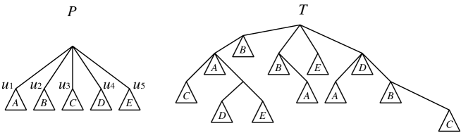
Figure 7: For these trees, $Occ(u_{1},M)=Occ(u_{2},M)=3$, $Occ(u_{3},M)=Occ(u_{4},M)=Occ(u_{5},M)=2$, $d_{2}=3$, $d_{3}=2$, and $occ(P,T)=3$,

Proposition 3.

Suppose that $P(u)$ has a leaf labeled with $b$. If $P(u)\subset T(v)$, then $v$ is an ancestor of a leaf (or leaf itself) with label $b$.

We say that $v_{j}$ is a minimal node for $u_{i}$ if $P(u_{i})\prec T(v_{j})$ holds. It follows from the proposition above that the number of minimal nodes is at most $k$ for each $u_{i}$ if $occ(P,T)=k$.

The preliminary version of this paper [5] showed that the case $k=2$ can be solved in polynomial time by using a reduction to 2-SAT. Here, we give a more direct solution that effectively utilizes some techniques from a classic polynomial-time algorithm for 2-SAT [8]. This algorithm will be extended for the case of $k=3$ in the next subsection.

From Proposition 2, it is enough to consider the decision of whether $P(u)\subset T(v)$ with $u$ corresponding to $v$. Let $Chd(u)=\{u_{1},\ldots,u_{d}\}$. We present a simple algorithm to decide whether or not $P(u)\subset T(v)$. We can assume by induction that $P(u_{i})\prec T(v_{j})$ is known for all $u_{i}\in Chd(u)$ and for all $v_{j}\in V(T(v))-\{v\}$. Let $M=\{(u_{i},v_{j})\,|\,P(u_{i})\prec T(v_{j})~{}\land~{}v_{j}\in V(T(v))\}$. We define $OCC(u_{i},M)$ and $Occ(u_{i},M)$ by

$$OCC(u_{i},M) = \{(u_{i},v_{j})\,|\,(u_{i},v_{j})\in M\}.$$

$$Occ(u_{i},M) = |OCC(u_{i},M)|.$$

See Fig. 7 for an illustration. A node $u_{i}$ with $Occ(u_{i},M)=h$ is called a node of rank $h$. Note that $u_{i}$, $v_{j}$, and $M$ appearing above depend on $(u,v)$.

The crucial task is to find an injective mapping $\psi$ (called a valid mapping) from $P(u)$ to $V(T(v))-\{v\}$ such that $P(u_{i})\prec T(\psi(u_{i}))$ holds for all $u_{i}$ ($i=1,\ldots,d$) and there is no ancestor/descendant relationship between any $\psi(u_{i})$ and $\psi(u_{j})$ ($u_{i}\neq u_{j}$). If this task can be performed in $O(f(d,m,n))$ time, from Proposition 2, the total time complexity will be $O^{\ast}(f(d,m,n))$. We assume w.l.o.g. that $\psi$ is given as a set of mapping pairs.

Hereafter, we let $Chd(u)=\{u_{i_{1}},\ldots,u_{i_{d}}\}$. Since we consider the case of $occ(P,T)$ $=2$, we assume w.l.o.g. that all $u_{i_{k}}$s have rank 2 (i.e., $Occ(u_{i_{k}},M)=2$ for $k=1,\ldots,d$). Accordingly, we let $OCC(u_{i_{k}},M)=\{(u_{i_{k}},v_{j_{k,0}}),(u_{i_{k}},v_{j_{k,1}})\}$ for $k=1,\ldots,$ $d$. As in [8], we construct a directed graph $G_{2}(V_{2},E_{2})$ by

$$V_{2} = \{u_{i_{k,0}},u_{i_{k,1}}\mid u_{i_{k}}\in Chd(u)\},$$

$$E_{2} = \{(u_{i_{k,p}},u_{i_{h,q}})\mid v_{j_{k,p}}\in AncDes(v_{j_{h,1-q}}),~{}h\neq k\},$$

where $u_{i_{k,p}}$s are newly introduced symbols. See also Fig. 8. Intuitively, an arc $(u_{i_{k,p}},u_{i_{h,q}})$ implies that if $(u_{i_{k}},v_{j_{k,p}})$ is in the inclusion mapping then it is possible for $(u_{i_{h}},v_{j_{h,q}})$, but not $(u_{i_{h}},v_{j_{h,1-q}})$, to be in the mapping, too.

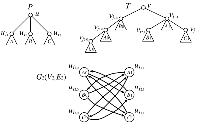
Figure 8: Example of $G_{2}(V_{2},E_{2})$ constructed from $P(u)$ and $T(v)$ in the case of $occ(P,T)=2$. Each vertex $u_{i_{k,p}}$ is represented by the corresponding subtree in $T$, where triangles labeled by the same capital letter represent isomorphic subtrees. $G_{2}(V_{2},E_{2})$ has two strongly connected components $\{u_{i_{1,0}},u_{i_{2,1}},u_{i_{3,1}}\}$ and $\{u_{i_{1,1}},u_{i_{2,0}},u_{i_{3,0}}\}$, whereas there is only one consistent assignment $\{u_{i_{1,0}}=1,u_{i_{2,1}}=1,u_{i_{3,1}}=1,u_{i_{1,1}}=0,u_{i_{2,0}}=0,u_{i_{3,0}}=0\}$, which corresponds to a mapping $\psi=\{(u_{i_{1}},v_{j_{1,0}}),(u_{i_{2}},v_{j_{2,1}}),(u_{i_{3}},v_{j_{3,1}})\}$.

Proposition 4.

There exists a path (resp., an edge) from $u_{i_{k,p}}$ to $u_{i_{h,q}}$ if and only if there exists a path (resp., an edge) from $u_{i_{h,1-q}}$ to $u_{i_{k,1-p}}$

Proof.

It is shown in [8] that $G_{2}(V_{2},E_{2})$ has a duality property: $G_{2}$ is isomorphic to the graph obtained from $G_{2}$ by reversing the direction of all the edges and complementing the names of all vertices. Since $u_{i_{h,q}}$ and $u_{i_{h,1-q}}$ (resp., $u_{i_{k,p}}$ and $u_{i_{k,1-p}}$) correspond to complementary variables, the proposition holds. ∎

Consider a 0-1 assignment to $V_{2}$, where 0 and 1 correspond to false and true, respectively. An assignment is called consistent if the following conditions are satisfied.

• $u_{i_{k,0}}+u_{i_{k,1}}=1$ holds for all $k=1,\ldots,d$,

• if $u_{i_{k,p}}=1$, all vertices reachable from $u_{i_{k,p}}$ have value 1.

Note that the first condition implies that $u_{i_{k,1-p}}$ corresponds to the negation of $u_{i_{k,p}}$, which further means that $u_{i_{k}}$ must be mapped to exactly one of $v_{j_{k,0}}$ and $v_{j_{k,1}}$. Note also that the second condition implies that if $u_{i_{k,p}}=0$, all vertices reachable to $u_{i_{k,p}}$ have value 0.

Proposition 5.

$P(u)\subset T(v)$ holds if and only if there exists a consistent assignment. Furthermore, $\psi$ can be obtained from the vertices to which 1 is assigned.

Proof.

Suppose that there exists a consistent assignment. Then, we can construct an inclusion mapping $\psi$ for $Chd(u)$ by letting $\psi(u_{i_{k}})=v_{j_{k.p}}$ for $p$ such that $u_{i_{k,p}}=1$, for all $u_{i_{k}}\in Chd(u)$, where the validity follows from the above two conditions and the meaning of an arc.

Conversely, suppose that there exists an inclusion mapping $\psi$. Then, we let $u_{i_{k,p}}=1$ if and only if $\psi(u_{i_{k}})=v_{j_{k.p}}$ for all $u_{i_{k}}\in Chd(u)$, which clearly satisfies the above two conditions. ∎

As in [8], we have the following proposition.

Proposition 6.

There exists a consistent assignment to $V_{2}$ if and only if there is no $k$ such that $u_{i_{k,0}}$ and $u_{i_{k,1}}$ belong to the same strongly connected component in $G_{2}(V_{2},E_{2})$.

The strongly connected components can be computed in linear time [29]. Furthermore, a consistent assignment can be obtained by greedily assigning 1 to vertices from deeper to shallower SCCs under the DFS (depth first search) ordering as in [8]. Since this procedure can clearly be done in polynomial time, the following theorem holds.

Theorem 3.

Unordered tree inclusion can be solved in polynomial time if $occ(P,$ $T)=2$.

6 An $O^{\ast}(1.619^{d})$-time algorithm for the case of $occ(P,T)=3$

In this section, we present an $O^{\ast}(1.619^{d})$-time algorithm for the case of $occ(P,T)=3$, where $d$ is the maximum degree of $P$, $m=|V(P)|$, and $n=|V(T)|$. Note that this case remains NP-hard from Theorem 2.

The basic strategy is to combine bottom-up dynamic programming and detection of a consistent assignment as in Section 5 to determine whether $P(u)\subset T(v)$ holds, where a recursive procedure is employed here for finding a consistent assignment. Let $Chd(u)=\{u_{i_{1}},\ldots,u_{i_{d}}\}$. As in Section 5, we can assume that $P(u_{i_{k}})\prec T(v_{j_{h}})$ is known for all $u_{i_{k}}$ and for all $v_{j_{h}}\in V(T(v))-\{v\}$, and we let $M=\{(u_{i_{k}},v_{j_{h}})\,|\,P(u_{i_{k}})\prec T(v_{j_{h}})~{}\land~{}v_{j_{h}}\in V(T(v))\}$.

Let $d_{3}$ (resp., $d_{2}$) be the number of $u_{i_{k}}$s of rank 3 (resp., rank 2) (see also Fig. 7). We assume w.l.o.g. that $d_{2}+d_{3}=d$ because $Occ(u_{i_{k}},M)=1$ means that $\psi(u_{i_{k}})$ is uniquely determined and thus we can ignore $u_{i_{k}}$s with $Occ(u_{i_{k}},M)=1$.

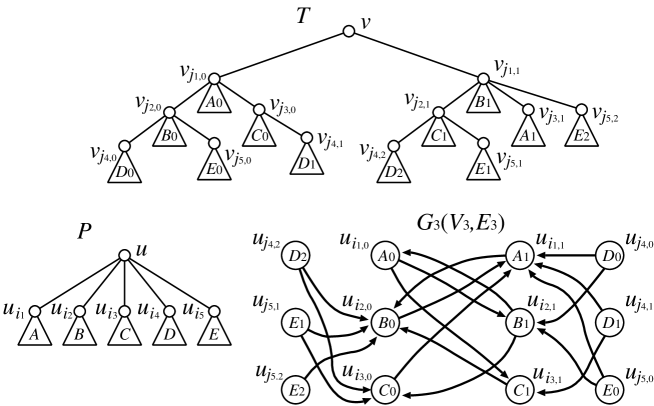
Figure 9: Example of $G_{3}(V_{3},E_{3})$ constructed from $P(u)$ and $T(v)$ in the case of $occ(P,T)=3$. $u_{j_{4,0}}$ and $u_{j_{5,0}}$ are inadmissible vertices, and $(u_{j_{4,1}},u_{j_{5,1}})$ is an inadmissible pair,

We construct $G_{2}(V_{2},E_{2})$ as in Section 5, using only $u_{i_{k}}$s with rank 2 and the corresponding $v_{j_{h}}$s, considering ancestor-descendant relations only among them. Then, for each $u_{i_{k}}\in Chd(u)$ such that $OCC(u_{i_{k}},M)=\{(u_{i_{k}},v_{j_{k,0}}),(u_{i_{k}},v_{j_{k,1}}),$ $(u_{i_{k}},v_{j_{k,2}})\}$, we let $V_{OCC3}(u_{i_{k}})=\{u_{i_{k,0}},u_{i_{k,1}},u_{i_{k,2}}\}$, where $u_{i_{k,p}}$s are newly introduced symbols. Let $V_{OCC3}=\bigcup_{Occ(u_{i_{k}},M)=3}V_{OCC3}(u_{i_{k}})$. Then, we construct $G_{3}(V_{3},E_{3})$ from $G_{2}(V_{2},E_{2})$ by

$$V_{3} = V_{2}\cup V_{OCC3},$$

$$E_{3} = E_{2}\cup\{(u_{i_{k,p}},u_{i_{h,q}})\mid u_{i_{k,p}}\in V_{OCC3},u_{i_{h,q}}\in V_{2},v_{i_{h,1-q}}\in AncDes(v_{i_{k,p}})\}.$$

See Fig. 9 for an example of $G_{3}(V_{3},E_{3})$.

Definition 2.

We say that $u_{i_{k,p}}\in V_{OCC3}$ is an inadmissible vertex if there exist paths from $u_{i_{k,p}}$ to $u_{i_{l,0}}$ and $u_{i_{l,1}}$ in $G_{3}(V_{3},E_{3})$ for some $u_{i_{l}}\in Chd(u)$ of rank 2. We also say that $(u_{i_{k,p}},u_{i_{h,q}})\in V_{OCC3}\times V_{OCC3}$ ($k\neq h$) is an inadmissible pair if $v_{i_{h,q}}\in AncDes(v_{i_{k,p}})$ holds, or there exist a path reachable from $u_{i_{k,p}}$ to $u_{i_{l,0}}$ in $G_{3}(V_{3},E_{3})$ and a path reachable from $u_{i_{h,q}}$ to $u_{i_{l,1}}$ in $G_{3}(V_{3},E_{3})$ for some $u_{i_{l}}\in Chd(u)$ of rank 2.

It is to be noted that an inadmissible vertex or an inadmissible pair $(u_{i_{k,p}},u_{i_{h,q}})$ cannot appear in any injective mapping $\psi$ for $P(u)\subset T(v)$ because the use of an inadmissible vertex or an inadmissible pair would make a consistent assignment impossible. Accordingly, we can assume w.l.o.g. that there does not exist an inadmissible vertex $u_{i_{k,p}}$ in $V_{OCC3}$.

Proposition 7.

Suppose that there exists a consistent assignment on vertices in $G_{2}(V_{2},E_{2})$ in the sense defined in Section 5. If there does not exist an inadmissible pair, there exists a valid mapping $\psi$. Furthermore, such a mapping can be found in polynomial time.

Proof.

We present a greedy algorithm for finding a consistent assignment, from which a valid mapping can be obtained. Beginning with an empty assignment on all vertices in $V_{2}$, we repeat the following procedure in any order: for each $u_{i_{k}}$ of rank 3, assign 1 to $u_{i_{k,0}}$, assign 0 to $u_{i_{k,1}}$ and $u_{i_{k,2}}$, and assign 1 to all vertices in $G_{3}(V_{3},E_{3})$ reachable from $u_{i_{k,0}}$. Finally, we extend the resulting assignment to a consistent assignment by assigning 1 to remaining vertices from deeper to shallower strongly connected components under the DFS ordering. Clearly, this algorithm works in polynomial time. It is also seen from the definition of the inadmissible pair that this algorithm always finds a consistent assignment. ∎

We denote the procedure in the proof of Proposition 7 by $FindMappingAD(M)$. This procedure returns true or false. true corresponds to the case where a consistent assignment and a valid mapping $\psi$ exist. It is straightforward to modify the procedure so that it outputs $\psi$ when it exists.

In order to handle inadmissible pairs, we employ a simple recursive procedure. Suppose that $(u_{i_{k,p}},u_{i_{h,q}})$ is an inadmissible pair. If we include $(u_{i_{k}},v_{j_{k,p}})$ in $\psi$, we cannot include $(u_{i_{h}},v_{j_{h,q}})$ in $\psi$. In this case, $d_{3}$ is decreased by 2. If we do not include $(u_{i_{k}},v_{j_{k,p}})$, we can delete this pair from $M$, which decreases $d_{3}$ by 1. Based on this idea, we obtain the following main procedure for the case of $occ(P,T)=3$. Note that if we include $(u_{i_{k}},v_{j_{k,p}})$ in $\psi$, all pairs $(u_{i_{k}},v_{j_{k,r}})$ with $r=0,1,2$ are removed from $M$. Furthermore, all pairs $(u_{i_{h}},v_{j_{h,q}})$ such that $v_{j_{h,q}}\in AncDes(v_{j_{k,p}})$ are removed from $M$, which may cause further removal. $Update(M,(u_{i_{k}},v_{j_{k,p}}))$ executes this updating procedure while making the corresponding 0-1 assignments on $G_{3}(V_{3},E_{3})$.

Algorithm 2 $FindMapping(M)$

  if there exists an inadmissible pair $((u_{i_{k}},v_{j_{k,p}}),(u_{i_{h}},v_{j_{h,q}}))$ then

     $M_{1}:=Update(M,(u_{i_{k}},v_{j_{k,p}}))$

     $M_{2}:=M-\{(u_{i_{k}},v_{j_{k,p}})\}$

     if $FindMapping(M_{1})=\textbf{true}{}$ then

        return  true

     else

        return  $FindMapping(M_{2})$

     end if

  end if

  return  $FindMappingAD(M)$

Theorem 4.

Unordered tree inclusion can be solved in $O^{\ast}(1.619^{d})$ time if $occ(P,$ $T)=3$.

Proof.

It follows from the discussions above that $FindMapping(M)$ correctly decides whether $P(u)\subset T(v)$ (when $u$ and $v$ have the same label). Therefore, we analyze the exponential factor (depending on $d$) of the time complexity of $FindMapping(M)$.

Let $f(k)$ denote the number of times that $FindMapping(M)$ is called when $k=|\{u_{i}\,|\,Occ(u_{i},M)=3\}|$. Clearly, if $k\leq 1$, $f(k)\leq 1$. Otherwise (i.e., $k\geq 2$), it may invoke two recursive calls: one with at most $k-2$ nodes of rank 3 and the other with at most $k-1$ nodes of rank 3. Therefore, we have

$$f(k) \leq f(k-1)+f(k-2),$$

from which $f(k)=O(1.619^{k})$ follows (c.f., Fibonacci number).

Since $d_{3}\leq d$ holds and both $FindMappingAD(M)$ and $Update(M,(u_{i_{k}},u_{j_{k,p}}))$ work in polynomial time per execution, the total time complexity is $O^{\ast}(1.619^{d})$. ∎

7 A randomized algorithm for the case of $h(P)=1$ and $h(T)=2$

Finally, we consider the case of $h(P)=1$ and $h(T)=2$, denoted by IncH2. This problem variant is NP-hard according to Corollary 1. We assume w.l.o.g. that the roots of $P$ and $T$ have the same unique label and thus they must match in any inclusion mapping.

Let $U=\{u_{1},\ldots,u_{d}\}$ be the set of children of $r(P)$. Let $v_{1},\ldots,v_{g}$ be the children of $r(T)$, and let $v_{i,1},\ldots,v_{i,n_{i}}$ be the children of each $v_{i}$.

First, we assume that $\ell(u_{i})\neq\ell(u_{j})$ holds for all $i\neq j$, where $\ell(v)$ denotes the label of $v$. This special case is denoted by IncH2U. Recall that IncH2U remains NP-hard from the condition of $occ(P)=1$ of Corollary 1.

IncH2U can be solved by a reduction to CNF SAT, different from the one mentioned in Section 5. (In fact, it can be considered as an inverse reduction of the one originally used to prove the NP-hardness of unordered tree inclusion by Kilpeläinen and Mannila [19].) For each $u_{i}$, we define $X^{POS}_{i}$ and $X^{NEG}_{i}$ by

$$X^{POS}_{i} = \{x_{j}\,|\,\ell(u_{i})=\ell(v_{j})\},$$

$$X^{NEG}_{i} = \{x_{j}\,|\,(\exists v_{j,k}\in Chd(v_{j}))(\ell(u_{i})=\ell(v_{j,k}))\}.$$

For each $u_{i}$, we construct a clause $C_{i}$ by

$$C_{i}=\left(\bigvee_{x_{j}\in X^{POS}_{i}}x_{j}\right)\lor\left(\bigvee_{x_{j}\in X^{NEG}_{i}}\overline{x_{j}}\right).$$

Then, the resulting SAT instance is $\{C_{1},\ldots,C_{d}\}$. Intuitively, $x_{j}=1$ corresponds to the case where $u_{i}$ is mapped to $v_{j}$, where $\ell(u_{i})=\ell(v_{j})$. Of course, multiple $v_{j}$s may correspond to $u_{i}$. However, it is enough to consider an arbitrary one.

Proposition 8.

IncH2U can be solved in $O^{\ast}(1.234^{d})$ time.

Proof.

First we prove the correctness of the reduction, where we assume w.l.o.g. that $r(P)$ is mapped to $r(T)$. Suppose that there exists an inclusion mapping $\phi$ from $V(P)$ to $V(T)$. Then, we let $x_{j}=1$ if $\phi(u_{i})=v_{j}$, and $x_{j}=0$ if $\phi(u_{i})=v_{j,k}$. An arbitrary assignment can be done on each of the other variables. Then, we can see that there is no inconsistency on the resulting assignment and all $C_{i}$s are satisfied. Conversely, suppose that there exists a satisfying assignment on $C_{i}$s. We let $\phi(u_{i})=v_{j}$ if $x_{j}=1$ and $\ell(u_{i})=\ell(v_{j})$. Otherwise, we can let $\phi(u_{i})=v_{j,k}$ for some $v_{j}$ such that $x_{j}=0$ and $\ell(u_{i})=\ell(v_{j,k})$. This $\phi$ gives an inclusion mapping.

Next we consider the time complexity. In order to solve the satisfiability instance, we use Yamamoto’s $O^{\ast}(1.234^{d})$-time algorithm for SAT with $d$ clauses [31]. Since the other parts can be done in polynomial time, we have the proposition. ∎

In order to solve IncH2, we combine two algorithms: (A1) a random sampling-based algorithm; and (A2) a modified version of the $O(d2^{d}mn^{2})$-time algorithm in Section 3.

For (A1), we employ the color-coding technique [7]. Let $d_{0}$ be the number of $u_{i}$s having unique labels, and let $d_{1}\leq d_{2}\leq\cdots\leq d_{h}$ be the multiplicities of the other labels in $U$. Define $\alpha=1-\frac{d_{0}}{d}$. Note that $d_{0}+d_{1}+\cdots+d_{h}=d$ and $d-d_{0}=\alpha d$ hold.

For each label $a_{i}$ with $d_{i}\geq 2$ (i.e., $i>0$), we relabel the nodes in $P$ having label $a_{i}$ by $a^{1}_{i},a^{2}_{i},\ldots,a^{d_{i}}_{i}$ in an arbitrary order. For each node $v$ in $T$ having label $a_{i}$, we assign $a^{j}_{i}$ ($j=1,\ldots,d_{i}$) to $v$ uniformly at random, and then apply the SAT-based algorithm for IncH2U. Let $M$ be the set of pairs in an inclusion mapping from $P$ to $T$. If all nodes of $T$ appearing in $M$ have different labels, a valid inclusion mapping can be obtained. This success probability is given by

$${\frac{d_{1}!}{d_{1}^{d_{1}}}}\cdot{\frac{d_{2}!}{d_{2}^{d_{2}}}}\cdots{\frac{d_{h}!}{d_{h}^{d_{h}}}}~{}\geq~{}{\frac{(\alpha d)!}{(\alpha d)^{(\alpha d)}}}.$$

This inequality can be proved by repeatedly applying

$${\frac{d_{1}!}{d_{1}^{d_{1}}}}\cdot{\frac{d_{2}!}{d_{2}^{d_{2}}}}~{}\geq~{}{\frac{(d_{1}+d_{2})!}{(d_{1}+d_{2})^{d_{1}+d_{2}}}},$$

which is seen from

$${\frac{(d_{1}+d_{2})^{d_{1}+d_{2}}}{d_{1}^{d_{1}}d_{2}^{d_{2}}}}~{}\geq~{}\left(\begin{array}[]{c}d_{1}+d_{2}\\ d_{1}\end{array}\right)~{}=~{}{\frac{(d_{1}+d_{2})!}{d_{1}!d_{2}!}}.$$

Since ${\frac{k!}{k^{k}}}\geq e^{-k}$ holds for sufficiently large $k$, the success probability is at least $e^{-\alpha d}$. Therefore, if we repeat the random sampling procedure $e^{\alpha d}$ times, the failure probability is at most $(1-e^{-{\alpha d}})^{e^{\alpha d}}\leq e^{-1}<{\frac{1}{2}}$ because $\ln\left[(1-{\frac{1}{x}})^{x}\right]=x\ln(1-{\frac{1}{x}})\leq x(-{\frac{1}{x}})=-1=\ln(e^{-1})$ holds for any $x>1$.

If we repeat the procedure $k(\log n)e^{\alpha d}$ times where $k$ is any positive constant (i.e., the total time complexity is $O^{\ast}(1.234^{d}\cdot e^{\alpha d})$), the failure probability is at most ${\frac{1}{n^{k}}}$.

For (A2), we modify the $O(d2^{d}mn^{2})$-time algorithm as follows. Recall that if there exist labels with multiplicity more than one, $S(v,v_{i})$ is a multi-set. In order to represent a multi-set, we memorize the multiplicity of each label. Then, the number of distinct multi-sets is given by

$$N(d_{0},\ldots,d_{h}) = 2^{d_{0}}\cdot\prod_{l=1}^{h}(d_{l}+1).$$

Since $d_{i}+1\leq 3^{\lceil d_{i}/2\rceil}$ holds for any $d_{i}\geq 2$, this number is bounded as follows:

$$N(d_{0},\ldots,d_{h}) \leq 2^{d_{0}}\cdot 3^{\lceil(d-d_{0})/2\rceil}.$$

Then, the time complexity of (A2) is $O^{\ast}(2^{(1-\alpha)d}\cdot 3^{(\alpha/2)d})$.

Since we can select the minimum of the time complexities of (A1) and (A2), the resulting time complexity is given by

$$\max_{\alpha}\min(O^{\ast}(1.234^{d}\cdot e^{\alpha d}),O^{\ast}(2^{(1-\alpha)d}\cdot 3^{(\alpha/2)d})).$$

Since $1.234^{d}\cdot e^{\alpha d}$ and $2^{(1-\alpha)d}\cdot 3^{(\alpha/2)d}$ are increasing and decreasing functions of $\alpha$, respectively, this maximum is attained when $1.234\cdot e^{\alpha}=2^{(1-\alpha)}\cdot 3^{(\alpha/2)}$. By numerical calculation, we have $\alpha\approx 0.42217$, from which the following theorem follows.

Theorem 5.

IncH2 can be solved in randomized $O^{\ast}(1.883^{d})$ time with probability at least $1-{\frac{1}{n^{k}}}$, where $k$ is any positive constant.

The above algorithm may be derandomized by using $k$-perfect hash families as in [7]. However, since the construction of a $k$-perfect hash family has a high complexity, the resulting algorithm would have a time complexity much worse than $O^{\ast}(2^{d})$.

8 Concluding remarks

We have presented a new algorithm for unordered tree inclusion running in $O^{\ast}(2^{d})$ time, thus reducing the exponent $2d$ in the previously best known bound on the time complexity [19] to $d$. However, the $2^{d}$-factor may not be optimal. For example, our randomized algorithm for the special case of $h(P)=1$ and $h(T)=2$ runs in $O^{\ast}(1.883^{d})$ time, which suggests that further improvements could be possible. However, we were unable to obtain an $O^{\ast}((2-\varepsilon)^{d})$-time algorithm for any constant $\varepsilon>0$, even when $h(P)=h(T)=2$. Similarly, we could not obtain an $O^{\ast}((2-\varepsilon)^{d})$-time algorithm for any constant $\varepsilon>0$ when $occ(P,T)=4$. Therefore, to develop an $O^{\ast}((2-\varepsilon)^{d})$-time algorithm for unordered tree inclusion or to prove an $\Omega(2^{d})$ lower bound (e.g., using recent techniques from [1, 2, 12] for proving lower bounds on various tree and sequence matching problems) is left as an open problem.

Future work includes generalizing our techniques and applying them to the extended tree inclusion problem mentioned in Section 1.2. This problem variant was introduced by Mori et al. [24] as a way to make unordered tree inclusion more useful for practical pattern matching applications. It asks for an optimal connected subgraph of $T$ (if any) that can be obtained by applying node insertion operations as well as node relabeling operations to $P$ while allowing non-uniform costs to be assigned to the different node operations. It was shown in [24] that the unrooted case can be solved in $O^{\ast}(2^{2d})$ time, and a further extension of the problem that also allows at most $K$ node deletion operations can be solved in $O^{\ast}((ed)^{K}K^{1/2}2^{2(dK+d-K)})$ time, where $e$ is the base of the natural logarithm.

References

- [1] Amir Abboud, Arturs Backurs, Thomas Dueholm Hansen, Virginia Vassilevska Williams, and Or Zamir. Subtree isomorphism revisited. In Proceedings of the 27th Annual ACM-SIAM Symposium on Discrete Algorithms, pages 1256–1271. SIAM, 2018.
- [2] Amir Abboud, Virginia Vassilevska Williams, and Oren Weimann. Consequences of faster alignment of sequences. In Proceedings of the 41st International Colloquium on Automata, Languages, and Programming - Part 1, pages 39–51. Springer, 2014.
- [3] Tatsuya Akutsu, Daiji Fukagawa, Magnús M. Halldórsson, Atsuhiro Takasu, and Keisuke Tanaka. Approximation and parameterized algorithms for common subtrees and edit distance between unordered trees. Theoretical Computer Science, 470:10–22, 2013.
- [4] Tatsuya Akutsu, Daiji Fukagawa, Atsuhiro Takasu, and Takeyuki Tamura. Exact algorithms for computing the tree edit distance between unordered trees. Theoretical Computer Science, 412(4-5):352–364, 2011.
- [5] Tatsuya Akutsu, Jesper Jansson, Ruiming Li, Atsuhiro Takasu, and Takeyuki Tamura. New and improved algorithms for unordered tree inclusion. In Proceedings of the 29th International Symposium on Algorithms and Computation, pages 27:1–27:12, 2018.
- [6] Tatsuya Akutsu, Takeyuki Tamura, Daiji Fukagawa, and Atsuhiro Takasu. Efficient exponential-time algorithms for edit distance between unordered trees. Journal of Discrete Algorithms, 25:79–93, 2014.
- [7] Noga Alon, Raphael Yuster, and Uri Zwick. Color-coding. Journal of the ACM, 42(4):844–856, 1995.
- [8] Bengt Aspvall, Michael F. Plass, and Robert Endre Tarjan. A linear-time algorithm for testing the truth of certain quantified boolean formulas. Information Processing Letters, 8(3):121–123, 1979.
- [9] Philip Bille. A survey on tree edit distance and related problems. Theoretical Computer Science, 337(1):217–239, 2005.
- [10] Philip Bille and Inge Li Gørtz. The tree inclusion problem: In linear space and faster. ACM Transactions on Algorithms, 7(3):38, 2011.
- [11] Mahdi Boroujeni, Mohammad Ghodsi, MohammadTaghi Hajiaghayi, and Saeed Seddighin. approximation of tree edit distance in quadratic time. In Proceedings of the 51st Annual ACM Symposium on the Theory of Computing, pages 709–720. ACM, 2019.
- [12] Karl Bringmann, Pawel Gawrychowski, Shay Mozes, and Oren Weimann. Tree edit distance cannot be computed in strongly subcubic time (unless APSP can). In Proceedings of the 29th Annual ACM-SIAM Symposium on Discrete Algorithms, pages 1190–1206. SIAM, 2018.
- [13] Lijun Chang, Xuemin Lin, Wenjie Zhang, Jeffrey Xu Yu, Ying Zhang, and Lu Qin. Optimal enumeration: Efficient top-k tree matching. Proceedings of the VLDB Endowment, 8(5):533–544, 2015.
- [14] Sara Cohen and Nerya Or. A general algorithm for subtree similarity-search. In 2014 IEEE 30th International Conference on Data Engineering, pages 928–939. IEEE, 2014.
- [15] Erik D. Demaine, Shay Mozes, Benjamin Rossman, and Oren Weimann. An optimal decomposition algorithm for tree edit distance. ACM Transactions on Algorithms, 6(1):2, 2009.
- [16] Michael R. Garey and David S. Johnson. Computers and Intractability – A Guide to the Theory of NP-Completeness. W. H. Freeman and Company, New York, 1979.
- [17] Minos Garofalakis and Amit Kumar. Xml stream processing using tree-edit distance embeddings. ACM Transactions on Database Systems, 30(1):279–332, 2005.
- [18] Minoru Kanehisa, Susumu Goto, Yoko Sato, Masayuki Kawashima, Miho Furumichi, and Mao Tanabe. Data, information, knowledge and principle: back to metabolism in kegg. Nucleic Acids Research, 42(D1):D199–D205, 2013.
- [19] Pekka Kilpeläinen and Heikki Mannila. Ordered and unordered tree inclusion. SIAM Journal on Computing, 24(2):340–356, 1995.
- [20] Pradap Konda, Sanjib Das, Paul Suganthan G.C., AnHai Doan, Adel Ardalan, Jeffrey R. Ballard, Han Li, Fatemah Panahi, Haojun Zhang, Jeff Naughton, Shishir Prasad, Ganesh Krishnan, Rohit Deep, and Vijay Raghavendra. Magellan: toward building entity matching management systems. Proceedings of the VLDB Endowment, 9(12):1197–1208, 2016.
- [21] Hanna Köpcke, Andreas Thor, and Erhard Rahm. Evaluation of entity resolution approaches on real-world match problems. Proceedings of the VLDB Endowment, 3(1-2):484–493, 2010.
- [22] Jiwei Li, Thang Luong, Dan Jurafsky, and Eduard H. Hovy. When are tree structures necessary for deep learning of representations? In Proceedings of the 2015 Conference on Empirical Methods in Natural Language Processing, EMNLP 2015, Lisbon, Portugal, September 17-21, 2015, pages 2304–2314, 2015.
- [23] Jiří Matoušek and Robin Thomas. On the complexity of finding iso-and other morphisms for partial k-trees. Discrete Mathematics, 108(1-3):343–364, 1992.
- [24] Tomoya Mori, Atsuhiro Takasu, Jesper Jansson, Jaewook Hwang, Takeyuki Tamura, and Tatsuya Akutsu. Similar subtree search using extended tree inclusion. IEEE Transactions on Knowledge and Data Engineering, 27(12):3360–3373, 2015.
- [25] Mateusz Pawlik and Nikolaus Augsten. Rted: a robust algorithm for the tree edit distance. Proceedings of the VLDB Endowment, 5(4):334–345, 2011.
- [26] Maciej Piernik and Tadeusz Morzy. Partial tree-edit distance. Poznan University of Technology, Tech. Rep. RA-10/2013, 2013.
- [27] Dennis Shasha, Jason T. L. Wang, Kaizhong Zhang, and Frank Y. Shih. Exact and approximate algorithms for unordered tree matching. IEEE Transactions on Systems, Man, and Cybernetics, 24(4):668–678, 1994.
- [28] Kuo-Chung Tai. The tree-to-tree correction problem. Journal of the ACM, 26(3):422–433, 1979.
- [29] Robert Endre Tarjan. Depth-first search and linear graph algorithms. SIAM Journal on Computing, 1(2):146–160, 1972.
- [30] Gabriel Valiente. Constrained tree inclusion. Journal of Discrete Algorithms, 3(2):431–447, 2005.
- [31] Masaki Yamamoto. An improved -time deterministic algorithm for SAT. In Proceedings of the 16th International Symposium on Algorithms and Computation, pages 644–653. Springer, 2005.
- [32] Mohammed Javeed Zaki. Efficiently mining frequent trees in a forest: Algorithms and applications. IEEE Transactions on Knowledge and Data Engineering, 17(8):1021–1035, 2005.
- [33] Kaizhong Zhang and Tao Jiang. Some MAX SNP-hard results concerning unordered labeled trees. Information Processing Letters, 49(5):249–254, 1994.
- [34] Kaizhong Zhang, Rick Statman, and Dennis Shasha. On the editing distance between unordered labeled trees. Information Processing Letters, 42(3):133–139, 1992.