Hybrid Inflation in Quasi-minimal Supergravity with Monotonic Inflationary Potential

Abstract

We show how supersymmetric hybrid inflation with scalar spectral index $n_{\rm s}\simeq 0.96-0.97$ is realized in the context of quasi-minimal supergravity if we insist that the inflationary potential not exhibit any local minima. We also address the problem of the initial conditions for both monotonic and non-monotonic inflationary potentials.

I Introduction

The simplest supersymmetric (SUSY) hybrid inflation model dvali with weak radiative corrections and minimal Kähler potential predicts a scalar spectral index $n_{\rm s}$ which lies close to 0.98. An advantage of this scenario is that inflation is realized for inflaton values well below the reduced Planck scale $m_{\rm P}\simeq 2.44\times 10^{18}~{}{\rm GeV}$ (which is set to 1 throughout the rest of the paper) and is insensitive to supergravity corrections due to a cancellation of the supergravity-induced inflaton mass squared term in such a minimal model copeland . Inclusion of the first correction involving the inflaton field in the Kähler potential destroys the cancellation and generates an inflaton mass squared which seriously affects the inflationary scenario even at weak coupling of the inflaton. Assuming that the mass squared of the inflaton is positive pana0 in order to avoid the generation of local minima in the inflationary potential the value of the spectral index increases and soon the spectrum of density perturbations turns from red to blue. If, instead, we overlook the danger of the inflaton being trapped in a local minimum and allow for a negative inflaton mass squared bastero we may lower the value of the spectral index to lie in the presently favored range $n_{\rm s}\simeq 0.96-0.97$ planckcosm .

Our purpose here is to explore in detail the range of the parameters for which the inflationary potential is with certainty monotonic in spite of the inflaton mass squared being negative and, of course, the characteristics of “observable” inflation are acceptable. The existence of a region in the parameter space where the local minimum of the inflationary potential disappears was known to the authors of bastero but apparently they decided to concentrate on the region exhiditing local extrema and examine the inflationary scenario taking place for inflaton field values smaller in size than the position of the local maximum. The region where the potential is monotonic is also qualitatively described in the numerical exploration of rehman0 but no particular attention is payed to it.

We also address the problem of the initial conditions tet of such hybrid inflation scenarios by invoking an early inflationary stage initial ; pana1 ; pana2 considering inflationary potentials which are either monotonic or non-monotonic. Obviously, the existence of a local minimum in the inflationary potential complicates this already difficult problem.

The structure of the paper is the following. In Sec. II we present the SUSY hybrid inflation model and determine the range of the parameters for which the inflationary potential is monotonic. Sec. III is devoted to the initial condition problem. Finally Sec. IV contains our conclusions.

II The SUSY Hybrid Inflation Model

For definiteness, we consider a SUSY model based on the left-right symmetric gauge group $G_{\rm{LR}}=SU(3)_{\rm c}\times SU(2)_{\rm L}\times SU(2)_{\rm R}\times U(1)_{B-L}$. The superfields of the model which are relevant for inflation are a gauge singlet $S$ and a conjugate pair of Higgs superfields $\Phi$ and $\bar{\Phi}$ belonging to the $(1,1,2)_{1}$ and $(1,1,2)_{-1}$ representations of $G_{\rm LR}$, respectively. Here the subscripts denote $U(1)_{B-L}$ charges. The fields $\Phi$ and $\bar{\Phi}$ acquire vacuum expectation values (VEVs) which break $G_{\rm LR}$ to the standard model gauge group $G_{\rm SM}$. In addition we impose a global $U(1)$ R symmetry under which $S$ and the superpotential have charge 1 with $\Phi$ and $\bar{\Phi}$ being neutral.

The superpotential component which is relevant for our discussion is

$$W=\kappa S\left(M^{2}-\Phi{\bar{\Phi}}\right)$$ (1)

with the Kähler potential taken to be

$$K=|S|^{2}+|\Phi|^{2}+|\bar{\Phi}|^{2}+\frac{\alpha}{4}|S|^{4}.$$ (2)

Here $M$ is a superheavy mass and $\kappa$, $\alpha$ are dimensionless constants which are all assumed to be real and positive.

The F-term potential turns out to be

$$V_{F}=\kappa^{2}V_{0}\exp{K}$$ (3)

with

$$V_{0} = |M^{2}-\Phi\bar{\Phi}|^{2}\left(\left(1+|S|^{2}+\frac{\alpha}{2}|S|^{4}\right)^{2}\frac{1}{1+\alpha|S|^{2}}\right.$$ (4)

$$\quad\quad\quad\quad\quad\quad\left.-3|S|^{2}+|S|^{2}\left(|\Phi|^{2}+|\bar{\Phi}|^{2}\right){\frac{}{}}\right)$$

$$+|S|^{2}\left(|\Phi|^{2}+|\bar{\Phi}|^{2}+4|\Phi|^{2}|\bar{\Phi}|^{2}\right)$$

$$-2M^{2}|S|^{2}\left(\Phi\bar{\Phi}+H.c.\right)$$

The SUSY minimum of the potential, $S=0,|\Phi|=|\bar{\Phi}|=M$ lies along the D-flat direction $\Phi=\bar{\Phi}^{*}$. For $|S|>|S_{\rm c}|\simeq M$, where $S_{\rm c}$ is a critical value of $S$, the masses squared of $\Phi$, $\bar{\Phi}$ are positive and as a consequence the choice $\Phi=\bar{\Phi}=0$ is stable. For $|S|<|S_{\rm c}|$, instead, an instability develops and the system moves towards the SUSY vacuum.

Using the $U(1)$ R symmetry we can rotate $S$ on the real axis. Then, we define a real scalar field $\sigma$

$$S=\frac{\sigma}{\sqrt{2}}$$ (5)

which is almost canonically normalized provided that its value remains well below unity in size. In terms of $\sigma$ the potential with $\Phi=\bar{\Phi}=0$ becomes

$$V_{F} \overset{\Phi=\bar{\Phi}=0}{=} \kappa^{2}M^{4}\left(\left(1+\frac{1}{2}\sigma^{2}+\frac{\alpha}{8}\sigma^{4}\right)^{2}\left(1+\frac{\alpha}{2}\sigma^{2}\right)^{-1}\right.$$ (6)

$$\quad\quad\quad\quad\left.-\frac{3}{2}\sigma^{2}\right)\exp\left({\frac{1}{2}\sigma^{2}+\frac{\alpha}{16}\sigma^{4}}\right).$$

If $\sigma$ satisfies the inequalities $1\gg\sigma^{2}>\sigma_{\rm c}^{2}\simeq 2M^{2}$, the potential in Eq. (6) may be approximated by its second-order expansion in $\sigma^{2}$

$$V_{F}\overset{\Phi=\bar{\Phi}=0}{\simeq}\kappa^{2}M^{4}\left(1-\frac{\alpha}{2}\sigma^{2}+\frac{1}{8}\left(1-\frac{7}{2}\alpha+2\alpha^{2}\right)\sigma^{4}\right)$$ (7)

which is dominated by the constant term and leads to a (hybrid) inflationary stage.

To the inflationary potential we add the contribution

$$V_{\rm{rad}}=\kappa^{2}M^{4}\left(\frac{\delta_{\phi}}{2}\right)\ln\frac{\sigma^{2}}{\sigma_{\rm c}^{2}}$$ (8)

from radiative corrections, where

$$\delta_{\phi}=N_{\phi}\frac{\kappa^{2}}{8\pi^{2}}$$ (9)

and $N_{\phi}=2$ is the dimensionality of the representation to which $\Phi$, $\bar{\Phi}$ belong. Note that this equation is accurate for $\sigma/\sigma_{\rm c}\gg 1$, which requires that $\kappa$ be not much smaller than about $0.01$. The potential during inflation is then taken to be

$$V_{\rm{inf}}=\kappa^{2}M^{4}\left(1+\frac{\delta_{\phi}}{2}\ln\frac{\sigma^{2}}{\sigma_{\rm c}^{2}}-\frac{\beta}{2}\sigma^{2}+\frac{\beta^{2}\gamma}{4\delta_{\phi}}\sigma^{4}\right).$$ (10)

Here

$$\beta=\alpha$$ (11)

is the negative mass squared of $\sigma$ in units of the false vacuum energy density $\kappa^{2}M^{4}$ ($i.e.,m_{\sigma}^{2}=-\kappa^{2}M^{4}\beta$) and

$$\gamma=\frac{\delta_{\phi}}{2\beta^{2}}\left(1-\frac{7}{2}\alpha+2\alpha^{2}\right).$$ (12)

We assume that $\alpha$ is sufficiently small ($\alpha\lesssim 0.3596$) such that $\gamma>0$.

The first, second, and third derivative of $V_{\rm inf}$ with respect to the inflaton field $\sigma$ are, respectively, given by

$$V_{\rm{inf}}^{\prime}=\kappa^{2}M^{4}\left(\frac{\delta_{\phi}}{\sigma}\right)\left(1-x+\gamma x^{2}\right),$$ (13)

$$V_{\rm{inf}}^{\prime\prime}=-\kappa^{2}M^{4}\left(\frac{\delta_{\phi}}{\sigma^{2}}\right)\left(1+x-3\gamma x^{2}\right),$$ (14)

and

$$V_{\rm{inf}}^{\prime\prime\prime}=2\kappa^{2}M^{4}\left(\frac{\delta_{\phi}}{\sigma^{3}}\right)\left(1+3\gamma x^{2}\right).$$ (15)

Here, we have introduced the variable

$$x\equiv\frac{\beta\sigma^{2}}{\delta_{\phi}}.$$ (16)

Then, from the above relations using the approximation $V_{\rm{inf}}\simeq\kappa^{2}M^{4}$ we obtain the slow-roll parameters

$$\epsilon\equiv\frac{1}{2}\left(\frac{V_{\rm inf}^{\prime}}{V_{\rm inf}}\right)^{2}\simeq\frac{1}{2}\delta_{\phi}\beta\frac{(1-x+\gamma x^{2})^{2}}{x},$$ (17)

$$\eta\equiv\frac{V_{\rm{inf}}^{\prime\prime}}{V_{\rm inf}}\simeq-\beta\frac{1+x-3\gamma x^{2}}{x}$$ (18)

and

$$\xi^{2}\equiv\frac{V_{\rm{inf}}^{\prime}V_{\rm{inf}}^{\prime\prime\prime}}{V^{2}_{\rm inf}}\simeq 2\beta^{2}\frac{1-x+\gamma x^{2}}{x^{2}}\left(1+3\gamma x^{2}\right).$$ (19)

From these equations, assuming that $x$ and $\gamma$ are not much larger than 1 and $\delta_{\phi}\ll 1$, we obtain $\epsilon\ll|\eta|$ and $\epsilon|\eta|\ll\xi^{2}$.

Inflation ends when $\sigma$ reaches the value $\sigma_{\rm{end}}$ with

$$\sigma_{\rm{end}}^{2}\simeq\max\{2M^{2},\delta_{\phi}\},$$ (20)

depending on whether termination of inflation occurs through the waterfall mechanism or because of the radiative corrections becoming strong ($|\eta|\simeq 1$).

Let the value of the inflaton field $\sigma$ at horizon exit of the pivot scale $k_{*}=0.05\ \rm{Mpc}^{-1}$ be $\sigma_{*}$, with $x_{*}$ being the corresponding value of the parameter $x$. The number $N_{*}$ of e-foldings in the slow-roll approximation for the period in which $\sigma$ varies between an initial value $\sigma_{*}$ and the final value $\sigma_{\rm{end}}$ corresponding, respectively, to the values $x_{*}$ and

$$x_{\rm{end}}\simeq\beta\max\{\frac{2M^{2}}{\delta_{\phi}},1\}$$ (21)

of the variable $x$ is given by

$$N_{*}\simeq\frac{1}{2\beta}\int_{x_{\rm{end}}}^{x_{*}}\frac{dx}{1-x+\gamma x^{2}}.$$ (22)

Moreover, the scalar spectral index $n_{\rm s}$ is obtained in terms of $\eta_{*}$, the slow-roll parameter $\eta$ evaluated at the value $x=x_{*}$, as follows:

$$n_{\rm s} \simeq 1+2\eta_{*}$$ (23)

$$\simeq 1-2\beta\frac{1+x_{*}-3\gamma x_{*}^{2}}{x_{*}}.$$

Its running $\alpha_{\rm s}\equiv dn_{\rm s}/d\ln{k}$ is

$$\alpha_{\rm s}\simeq-2{\xi_{*}}^{2}\simeq-4\beta^{2}\frac{1-x_{*}+\gamma x_{*}^{2}}{x_{*}^{2}}\left(1+3\gamma x_{*}^{2}\right),$$ (24)

where $\xi_{*}^{2}$ is the parameter $\xi^{2}$ evaluated at horizon exit of the pivot scale. The scalar potential on the inflationary path can be written in terms of the scalar power spectrum amplitude $A_{\rm s}$ and the value $\epsilon_{*}$ of the slow-roll parameter $\epsilon$, both evaluated at horizon exit of the pivot scale, as

$$V_{\rm{inf}}=24\pi^{2}\epsilon_{*}A_{\rm s},$$ (25)

from which we obtain

$$M^{4}\simeq 3\beta\left(\frac{N_{\phi}}{2}\right)\frac{(1-x_{*}+\gamma x_{*}^{2})^{2}}{x_{*}}A_{\rm s}.$$ (26)

Finally, the tensor-to-scalar ratio is

$$r=16\epsilon_{*}\ll 1.$$ (27)

From Eq. (13) it follows that

$$\sigma V_{\rm{inf}}^{\prime}=\kappa^{2}M^{4}\delta_{\phi}\left(1-x+\gamma x^{2}\right).$$ (28)

Thus, it becomes apparent that $\sigma V_{\rm{inf}}^{\prime}$ is not necessarily positive for all values of the field $\sigma$ satisfying $\sigma/\sigma_{\rm c}>1$. If $4\gamma<1$ the polynomial $1-x+\gamma x^{2}$ is negative for all values of $x$ lying between its two distinct real and positive roots. The smallest root $x_{-}$ corresponds to a value of $|\sigma|$ where $V_{\rm{inf}}$ has a local maximum with the largest root $x_{+}$ corresponding to a value of $|\sigma|$ where $V_{\rm{inf}}$ has a local minimum. In this case a viable inflationary scenario may take place for values of the inflaton field corresponding to values of $x<x_{-}$ with $x_{-}\simeq 1$ for $\gamma\ll 1$. There is always the danger, however, of the inflaton being trapped in values corresponding to $x>x_{-}$ and ending up in the local minimum of $V_{\rm{inf}}$.

In the present work we intend to investigate the possibility of having a viable inflationary scenario in which $\sigma V_{\rm{inf}}^{\prime}\geq 0$ holds for all $\sigma/\sigma_{\rm c}>1$. From Eq. (28) $\sigma V_{\rm{inf}}^{\prime}\geq 0$ is achieved if we assume that $4\gamma\geq 1$ such that the polynomial $1-x+\gamma x^{2}$ has either a double real root or a pair of complex conjugate roots. It still holds but as a strict inequality $\sigma V_{\rm{inf}}^{\prime}>0$ if in the expansion of the potential we include terms up to $\sigma^{10}$ the coefficients of which are positive provided $\alpha\lesssim 0.9$. Moreover, it can be shown that the exact expression for $\sigma V_{F}^{\prime}$ derived from Eq. (6) is positive for $|\sigma|>\sqrt{2\beta/(1-3\alpha/2)}$. Since, as it turns out, we will be interested in $\beta\lesssim 0.01-0.02$ we conclude that the possible extema of the potential occur for values of $\sigma$ for which the analysis based on the expansion of the potential during inflation to order $\sigma^{10}$ is reliable.

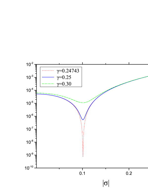
Figure 1: The exact value of $\sigma V_{F}^{\prime}/(\kappa^{2}M^{4})$ during inflation with the radiative corrections included as a function of the absolute value of the field $\sigma$ for $\alpha=0.01$ and $\gamma=0.24743,0.25,0.30$.

In Fig. 1 we plot $\sigma V_{F}^{\prime}/(\kappa^{2}M^{4})$ using the exact expression derived from Eq. (6) for $\alpha=0.01$ and $\gamma=0.24743$,$0.25,0.30$ with the radiative corrections included. For larger values of $|\sigma|$ than the ones presented in the graph $\sigma V_{F}^{\prime}$ is certainly positive according to our earlier discussion. We find a minimum at $|\sigma|\simeq 0.101$ which is very close to the $\gamma$-independent location

$$|\sigma_{\rm m}|=\sqrt{\beta/(1-7\alpha/2+2\alpha^{2})}$$ (29)

of the minimum of the approximate expression given in Eq. (28). The value of $\sigma V_{F}^{\prime}$ at the minimum, however, is not zero for $\gamma=0.25$ but for a slightly smaller value of $\gamma$ which is close to $\gamma=0.24743$ for $\alpha=0.01$. As $\alpha$ decreases the vanishing of $\sigma V_{F}^{\prime}$ occurs for values of $\gamma$ closer to $\gamma=0.25$. Thus, it is confirmed that the inflationary potential for $\gamma\geq 0.25$ is strictly monotonic.

For values of $|\sigma|$ close to $|\sigma_{\rm m}|$, where $\sigma V_{F}^{\prime}$ is minimized and is close to zero for $\gamma\simeq 0.25$, the effect of higher order terms in the expansion of the potential in powers of $\sigma^{2}$ may not be negligible. However, this will not affect the “observable” inflation if $|\sigma_{*}|$ is sufficiently smaller than $|\sigma_{\rm m}|$. We expect that this will be the case because of the enhanced flatness of the potential for $|\sigma|$ close to $|\sigma_{\rm m}|$.

We first consider the very important special case $\gamma=1/4$ which is amenable to simple analytic treatment. For this value of $\gamma$

$$1-x+\gamma x^{2}=\frac{1}{4}(2-x)^{2}$$ (30)

and

$$1+x-3\gamma x^{2}=\frac{1}{4}(2-x)(2+3x).$$ (31)

Let us also assume, as it can be verified a posteriori, that

$$x_{\rm{end}}\simeq\beta\ll 1.$$ (32)

Then,

$$N_{*}\simeq\frac{1}{\beta}\left(\frac{x_{*}}{2-x_{*}}\right)-\frac{1}{2}$$ (33)

and

$$n_{\rm s} \simeq 1-\beta\left(\frac{2-x_{*}}{x_{*}}\right)\left(1+\frac{3}{2}x_{*}\right)$$ (34)

$$\simeq 1-\left(1+\frac{3}{2}x_{*}\right)\left(N_{*}+\frac{1}{2}\right)^{-1}.$$

From the above equations we easily obtain

$$x_{*}\simeq\frac{2}{3}\left(\left(N_{*}+\frac{1}{2}\right)\left(1-n_{\rm s}\right)-1\right)$$ (35)

and

$$\beta\simeq\left(\frac{x_{*}}{2-x_{*}}\right)\left(N_{*}+\frac{1}{2}\right)^{-1}.$$ (36)

Thus, we are able to compute $x_{*}$ and $\beta=\alpha$ with $N_{*}$ and $n_{\rm s}$ as inputs. Finally, using the values of $\gamma$, $\beta=\alpha$ and $x_{*}$ we may derive the value of the coupling $\kappa$ and the absolute value $|\sigma_{*}|$ of the inflaton field at horizon exit of the pivot scale. In particular, it holds that

$$\kappa^{2}\simeq(4\gamma)\left(\frac{8\pi^{2}}{N_{\phi}}\right)\frac{\beta^{2}}{2-7\alpha+4\alpha^{2}}$$ (37)

and

$$\sigma_{*}^{2}\simeq(4\gamma)\frac{x_{*}\beta}{2-7\alpha+4\alpha^{2}}.$$ (38)

As $n_{\rm s}$ decreases with $N_{*}$ kept fixed both $x_{*}$ and $\beta$ increase (assuming $x_{*}<2$) and from the above equations both $\kappa$ and $|\sigma_{*}|$ also increase provided, of course, that $\beta=\alpha<0.3596<7/8$.

Throughout the subsequent discussion we make the choice $N_{*}=50$, in order to solve the horizon and flatness problems for reheat temperature $T_{\rm r}\sim 10^{9}~{}{\rm GeV}$, and also set $N_{\phi}=2$ and $A_{\rm s}=2.215\times 10^{-9}$ planckcosm .

Then, for $\gamma=1/4$ and $n_{\rm s}=0.96$ we obtain $x_{*}\simeq 0.68$, $\beta=\alpha\simeq 0.0102$, $\kappa\simeq 0.0461$, $|\sigma_{*}|\simeq 0.06$, $|\sigma_{\rm m}|\simeq 0.1028$, $\alpha_{\rm s}\simeq-5.28\times 10^{-4}$, and $M\simeq 2.086\times 10^{-3}$. If, instead, $n_{\rm s}=0.97$ we obtain $x_{*}\simeq 0.3433$, $\beta=\alpha\simeq 0.0041$, $\kappa\simeq 0.0184$, $|\sigma_{*}|\simeq 0.0267$, $|\sigma_{\rm m}|\simeq 0.0645$, $\alpha_{\rm s}\simeq-4.27\times 10^{-4}$, and $M\simeq 2.473\times 10^{-3}$. Finally, we may also consider the value $n_{\rm s}=0.95$ although at present it does not seem to be favored by the cosmological data. It gives $x_{*}\simeq 1.0167$, $\beta=\alpha\simeq 0.02047$, $\kappa\simeq 0.0944$, $|\sigma_{*}|\simeq 0.1058$, $|\sigma_{\rm m}|\simeq 0.1485$, $\alpha_{\rm s}\simeq-6.96\times 10^{-4}$, and $M\simeq 1.672\times 10^{-3}$.

Let us now turn to the more general case where $\gamma>1/4$. From Eq. (23) we obtain

$$x_{*}\simeq\frac{n_{\rm s}+2\beta-1+\sqrt{\left(1-n_{\rm s}-2\beta\right)^{2}+48\beta^{2}\gamma}}{12\beta\gamma}.$$ (39)

Also from Eq. (22), assuming again that $x_{\rm{end}}\simeq\beta$, we get

$$N_{*}\simeq\frac{1}{\beta\sqrt{4\gamma-1}}\left(\arctan\frac{1-2\beta\gamma}{\sqrt{4\gamma-1}}-\arctan\frac{1-2x_{*}\gamma}{\sqrt{4\gamma-1}}\right).$$ (40)

If the value of $x_{*}$ from Eq. (39) is used in Eq. (40) we obtain $N_{*}$ as a function of $\beta$ for a given value of $n_{\rm s}$. Thus, the value of $\beta$ can be determined (numerically) as the one which gives the desirable value of $N_{*}$. In the event that there are more than one such values we choose the smallest one because it leads to the smallest value of $|\sigma_{*}|$. The determination of the remaining parameters proceeds as in the previous case.

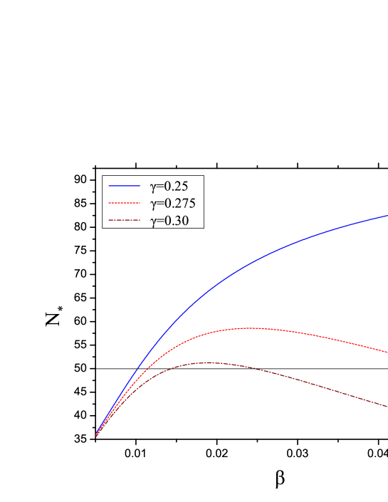
Figure 2: The number $N_{*}$ of e-foldings as a function of $\beta$ with $n_{\rm s}=0.96$ for $\gamma=$ $0.25,0.275,0.30$.

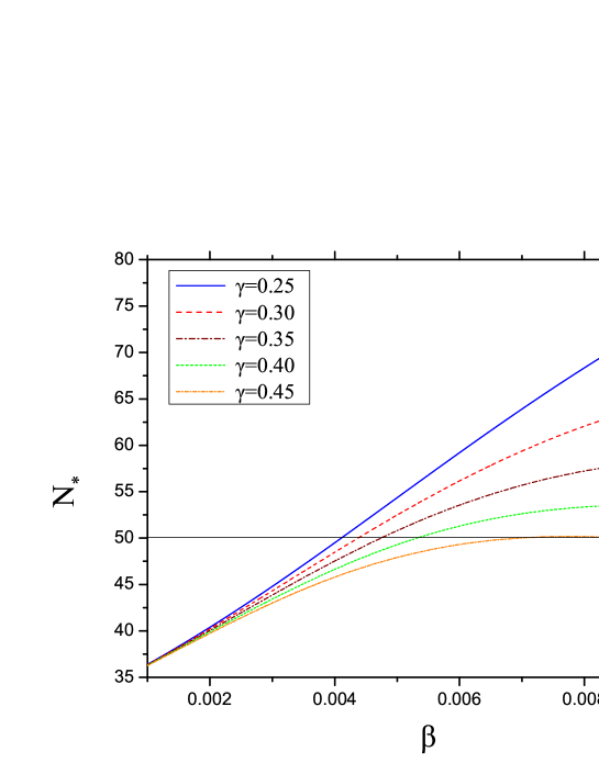
Figure 3: The number $N_{*}$ of e-foldings as a function of $\beta$ with $n_{\rm s}=0.97$ for $\gamma=$ $0.25,0.30,0.35,0.40,0.45$.

In Fig. 2 we plot the number of e-foldings $N_{*}$ as a function of the parameter $\beta$ for $\gamma=0.25,0.275,0.30$ assuming $n_{\rm s}=0.96$. Given our requirement that $N_{*}=50$, values of $\gamma\gtrsim 0.30$ should not be considered. The chosen value $N_{*}=50$ seems to be attained for each allowed value of $\gamma$ at two different values of $\beta$ out of which we accept the smallest one. We see that $\beta$ lies in the range $\sim 0.01-0.015$. Similarly, in Fig. 3 we plot $N_{*}$ as a function of $\beta$ for $\gamma=0.25,0.30,0.35,0.40,0.45$ assuming $n_{\rm s}=0.97$. We see that with $n_{\rm s}$ increasing the allowed range of values of $\gamma$ becomes larger while the range of the parameter $\beta$ is shifted towards smaller values. For $n_{\rm s}=0.97$ the range of $\beta$ is $\sim 0.004-0.007$.

Let us consider the case where $\gamma=0.30$, a value allowed for all values of $n_{\rm s}$ in the range $0.96-0.97$. If $n_{\rm s}=0.96$ we obtain $x_{*}\simeq 0.8587$, $\beta=\alpha\simeq 0.01437$, $\kappa\simeq 0.0718$, $\alpha_{\rm s}\simeq-6.75\times 10^{-4}$, $|\sigma_{*}|\simeq 0.0883$, $|\sigma_{\rm m}|\simeq 0.1231$, and $M\simeq 1.955\times 10^{-3}$. If, instead, $n_{\rm s}=0.97$ we get $x_{*}\simeq 0.3628$, $\beta=\alpha\simeq 0.00437$, $\kappa\simeq 0.0214$, $\alpha_{\rm s}\simeq-4.4\times 10^{-4}$, $|\sigma_{*}|\simeq 0.0311$, $|\sigma_{\rm m}|\simeq 0.0666$, and $M\simeq 2.461\times 10^{-3}$.

We also give results for $\gamma=0.45$ which is close to the largest allowed value of $\gamma$ for $n_{\rm s}=0.97$. We have $x_{*}\simeq 0.5323$, $\beta=\alpha\simeq 0.00694$, $\kappa\simeq 0.0419$, $\alpha_{\rm s}\simeq-5.6\times 10^{-4}$, $|\sigma_{*}|\simeq 0.0584$, $|\sigma_{\rm m}|\simeq 0.0843$, and $M\simeq 2.354\times 10^{-3}$.

One conclusion that can be drawn from Figs. 2 and 3 and is confirmed by the numerical results presented above is that given $n_{\rm s}$ the inflationary scenario with monotonic $V_{\rm{inf}}$ having the lowest value of $\beta=\alpha$, the smallest coupling $\kappa$, and the smallest inflaton field value $|\sigma_{*}|$ is obtained for the smallest value of $\gamma$, namely $\gamma=1/4$. This demonstrates the importance of this special case for which it just so happens that it can be treated fully analytically.

III The initial conditions

The above discussion of the hybrid inflationary scenario is certainly simplified since it is restricted to field values along the inflationary trajectory $\Phi=\bar{\Phi}=0$. The naturalness of the scenario, however, depends on the existence of field values which although initially are far from the inflationary trajectory they approach it during the subsequent evolution. We assume that the energy density $\rho$ of the universe is dominated by the F-term potential $V_{F}$ in Eq. (3). To evade the steep region of the potential generated by supergravity we require that all field values are well below unity in magnitude such that we are allowed to neglect, to a first approximation, terms of dimension higher than four in $V_{F}$. Let us start away from the inflationary trajectory and choose the initial energy density $\rho_{0}$ to satisfy the relation $\kappa^{2}M^{4}\ll\rho_{0}\lesssim 1.$ Moreover, we assume that $|\Phi|,|\bar{\Phi}|$ start somewhat below $|S|$. Then, $V_{F}\sim\kappa^{2}|S|^{2}\left(|\Phi|^{2}+|\bar{\Phi}|^{2}\right)$. We would like $\Phi,\bar{\Phi}$ to oscillate from the beginning as massive fields due to their coupling to $S$ and quickly approach zero. In contrast, $|S|$ should stay considerably larger than $|S_{c}|\simeq M$. Thus, initially it must certainly hold that ${m_{S}^{2}}\lesssim V_{F}\lesssim{m_{\Phi,{\bar{\Phi}}}^{2}}$ or $|\Phi|^{2}+|\bar{\Phi}|^{2}\lesssim 1\lesssim|S|^{2}$ which contradicts our assumption that $|S|<1$. Then we are left with the choice $\rho_{0}\sim\kappa^{2}M^{4}$. In this case $|S|$ remains larger than $|S_{\rm c}|$ provided ${m_{S}^{2}}\lesssim{\kappa^{2}M^{4}}$ or $|\Phi|^{2}+|\bar{\Phi}|^{2}\lesssim M^{4}$. We see that we are forced to start very close to the inflationary trajectory and severely fine tune the starting field configuration tet .

This severe fine tuning becomes more disturbing since the field configuration at the assumed onset of inflation should be homogeneous over dinstances $\sim H_{\rm{inf}}^{-1}$, where $H_{\rm{inf}}$ is the Hubble parameter $H$ at the onset of inflation. Homogeneity over a Hubble distance, however, is a justified assumption only if it concerns the end of the Planck era ($\rho_{0}\simeq 1$) where initial conditions should be set. Homogeneity over distances $\sim H_{\rm{inf}}^{-1}$ at the assumed onset of inflation is a natural consequence of homogeneity over distances $\sim{H_{0}}^{-1}$ at the end of the Planck era if during the intervening period the universe expands by at least a factor $H_{\rm{inf}}^{-1}/{H_{0}}^{-1}$ which corresponds to a minimum required number

$$N_{\rm{req}}=\frac{1}{2}\ln\frac{\rho_{0}}{\rho_{\rm{inf}}}$$ (41)

of e-foldings of expansion of the scale factor $R$. According to the expansion law $R\sim\rho^{-\frac{1}{3\gamma_{\rm e}}}$, however, the number of e-foldings is

$$N_{\rm{\gamma_{\rm e}}}=\frac{1}{3\gamma_{\rm e}}\ln\frac{\rho_{0}}{\rho_{\rm{inf}}}.$$ (42)

Typically, $\gamma_{\rm e}\gtrsim 1$ and consequently $N_{\rm{req}}>N_{\rm{\gamma_{\rm e}}}$. This means that the initial field configuration must be very homogeneous over $d_{\rm{hom}}$ Hubble lengths with

$$d_{\rm{hom}}\sim e^{N_{\rm{req}}-N_{\rm{\gamma_{\rm e}}}}=\left(\frac{\rho_{0}}{\rho_{\rm{inf}}}\right)^{\frac{3\gamma_{\rm e}-2}{6\gamma_{\rm e}}}\gg 1.$$ (43)

Such a homogeneity is hard to understand unless an early period of inflation took place at $\rho\sim 1$ initial ; pana1 ; pana2 with a number of e-foldings

$$N_{\rm{early}}\geq\frac{3\gamma_{\rm e}-2}{6\gamma_{\rm e}}\ln\frac{\rho_{0}}{\rho_{\rm{inf}}}+\frac{1}{3\gamma_{\rm e}}\ln\frac{\rho_{1}}{\rho_{2}}.$$ (44)

Here $\rho_{1}=\rho_{\rm{beg}}$ and $\rho_{2}=\rho_{\rm{end}}$ where $\rho_{\rm{beg}}$ ($\rho_{\rm{end}}$) is the energy density at the beginning (end) of the early inflation. Notice that in Eq. (44) $N_{\rm{early}}$ could be taken to be the number of e-foldings of expansion for any period during which $\rho$ varies from $\rho_{1}$ to $\rho_{2}$ with $\rho_{0}\geq\rho_{1}\geq\rho_{\rm{beg}}$ and $\rho_{\rm{end}}\geq\rho_{2}\geq\rho_{\rm{inf}}$. Setting $\rho_{1}=\rho_{0}$ and $\rho_{2}=\rho_{\rm{inf}}$ the right-hand-side (r.h.s) of Eq. (44) becomes $N_{\rm{req}}$. An early inflationary stage might also eliminate the requirement of severe fine tuning of the field configuration at $\rho=\rho_{0}$ since, in addition to the homogenization of space, it could alter the dynamics of the evolution of the universe during the period prior to (the later) inflation.

An inflation taking place at energy density $\rho_{\rm{early}}\gg\rho_{\rm{inf}}$, however, although eliminates existing inhomogeneities it generates new ones due to quantum fluctuations. Requiring that the gradient energy density resulting from these fluctuations not to exceed $\rho_{\rm{inf}}$ when $\rho\sim\rho_{\rm{inf}}$ gives an upper bound on the energy density $\rho_{\rm{early}}$ (towards the end) of the first stage of inflation pana2

$$\rho_{\rm{early}}\lesssim\left(6\pi\right)^{\frac{3\gamma_{\rm e}}{3\gamma_{\rm e}-1}}\rho_{\rm{inf}}^{\frac{3\gamma_{\rm e}-2}{2(3\gamma_{\rm e}-1)}}\qquad\left(\gamma_{\rm e}\gtrsim 1\right)$$ (45)

which is somewhat lower than unity and decreases with $\rho_{\rm{inf}}$.

For the role of the early inflation we are going to employ the “chaotic” D-term inflation of pana1 pana2 . Let $Z$ be a $G_{\rm{LR}}$-singlet chiral superfield with charge $-1$ under an “anomalous” $U(1)$ gauge symmetry. The D-term associated with it is

$$V_{D}=\frac{g^{2}}{2}\left({K_{Z}}Z-\xi\right)^{2}$$ (46)

with $K_{Z}$ denoting the derivative of the Kähler potential with respect to $Z$. If during some period of time $\left|{K_{Z}}{Z}\right|\ll\xi$ the D-term potential becomes approximately constant

$$V_{D}\simeq\frac{1}{2}g^{2}\xi^{2}$$ (47)

and on the condition that this constant dominates the energy density the universe experiences a period of quasi-exponential expansion. In the standard D-term inflation $\left|{K_{Z}}{Z}\right|$ is kept small because the scalar field $Z$ finds itself lying close to zero trapped in a wrong vacuum. In the “chaotic” D-term inflation, instead, $Z$ is not trapped in a wrong vacuum and its initial value does not have to be small. The version of “chaotic” D-term inflation that we consider here and which we are going to review briefly relies on a rather specific value of the the Fayet-Iliopoulos $\xi$ term pana2 .

Let us consider the double-well potential

$$V_{D}=\frac{g^{2}}{2}\left(\frac{\zeta^{2}}{2}-\xi\right)^{2}$$ (48)

involving the real scalar field $\zeta$ with canonically normalized kinetic term. This is the “anomalous” D-term potential of a field $Z$ with a minimal Kähler potential which is brought to the real axis ($Z=\mathsf{Re}Z=\frac{\zeta}{\sqrt{2}}$) by a gauge transformation under the “anomalous” $U(1)$ . For $|\zeta|\gg 1$, as well-known, the equation of motion

$$\frac{dv}{d\zeta}+\sqrt{3\left(\frac{1}{2}v^{2}+V\right)}+\frac{V^{\prime}}{v}=0$$ (49)

with

$$v\equiv\dot{\zeta}\equiv\frac{d\zeta}{dt}$$ (50)

admits the approximate inflationary slow-roll solution

$$v=-\sqrt{\frac{2}{3}}g\zeta.$$ (51)

For the specific value

$$\xi=\frac{1}{3},$$ (52)

however, the energy $E=\frac{1}{2}v^{2}+V$ calculated for the above solution becomes a “perfect square” and the approximate slow-roll solution becomes exact. Integration of this exact solution then leads to

$$\zeta=\zeta_{0}e^{-\sqrt{\frac{2}{3}}gt}$$ (53)

which demonstrates that $\zeta$ does not oscillate but vanishes only asymptotically with time. Moreover, the condition for inflationary expansion $-{\dot{H}}/{H^{2}}=3{E_{k}}/{E}<1$, where $E_{k}=v^{2}/2$ and $H=\sqrt{{E}/{3}}$, is violated only for $|\zeta|$ in the interval [$r_{-},r_{+}$] with $r_{\pm}=\sqrt{2}\pm 2/\sqrt{3}$.

Starting from a relatively large $\left|\zeta\right|$ the evolution of the field $\zeta$ approaches the solution in Eq. (53) giving rise to a “chaotic” inflationary expansion. After a short break of the inflationary expansion near the minimum of the potential a new inflationary expansion begins as $\zeta$ approaches the origin. This approach, however, is combined with a gradual departure from the non-oscillatory solution. Eventually, $\zeta$ will either stop before reaching the origin or cross the origin with a small speed. Then, a new inflationary expansion begins as $\zeta$ moves away from the origin. The duration of the inflationary stages at $\left|\zeta\right|\ll 1$ will, of course, depend on the accuracy with which the evolution of the field $\zeta$ follows the special solution in Eq. (53) which in turn depends on the duration of the inflationary stage at $\left|\zeta\right|\gg 1$.

The above discussion concentrates on the “anomalous” D-term which is assumed to be dominant during the initial stages of the evolution. This assumption certainly places constraints on the size of the initial values of all fields present in the model including the $Z$ field itself since they are all involved in the F-term potential. A noticeable contribution of $Z$ to the F-term potential is the exponential factor $e^{\frac{\zeta^{2}}{2}}$. As a consequence of the constraints on the initial value of $\zeta$ only a very short inflation at $\left|\zeta\right|\gg 1$ is allowed which necessitates the additional short inflationary stage at $\left|\zeta\right|\ll 1$ to complement the required expansion and solve the problem of the initial conditions.

To minimize the involvement of the $G_{\rm{LR}}$-singlet $Z$ in the F-term potential we assume that it does not enter the superpotential at all because of the charge assignments of the remaining fields under the “anomalous” $U(1)$ gauge symmetry. In particular, $S,\Phi,\bar{\Phi}$ are singlets under the “anomalous” $U(1)$. Moreover, we supplement the Kähler potential in Eq. (2) with the term

$$\delta K=|Z|^{2}-\xi.$$ (54)

Then, the F-term potential becomes

$$V_{F}=\kappa^{2}\left(V_{0}+|M^{2}-\Phi\bar{\Phi}|^{2}|Z|^{2}|S|^{2}\right)\exp(K+\delta K).$$ (55)

Minimization of the potential with respect to $Z$ at fixed $S$ satisfying $1\gg|S|>|S_{\rm c}|\simeq M$ and with $\Phi=\bar{\Phi}=0$ (which is again a stable choice) essentially amounts to minimizing the “anomalous” D-term provided that

$$\frac{1}{2}g^{2}\xi^{2}\gg\kappa^{2}M^{4}.$$ (56)

This gives $|Z|^{2}=\xi$ and leads to the F-term (hybrid) inflationary potential which is again approximated as in Eq. (10) but now with

$$\beta=\alpha-\xi$$ (57)

and

$$\gamma=\frac{\delta_{\phi}}{2\beta^{2}}\left(1-\frac{7}{2}\alpha+2\alpha^{2}+2\xi\right).$$ (58)

In the various scenarios concerning the “observable” inflation with $\gamma$, $N_{*}$ and $n_{\rm s}$ taken as inputs, the values of $\beta$, $x_{*}$, $\alpha_{\rm s}$ and $M$ remain the same, $\alpha$ is determined in terms of $\beta$ as $\alpha=\beta+\xi$, and $\kappa$ and consequently $|\sigma_{*}|$ increase slightly due the modified relation defining $\gamma$ given in Eq. (58). This slight change of $\kappa$ affects only the value of the slow-roll parameter $\epsilon$ which, however, does not lead to a detectable modification of the inflationary scenario since $\epsilon$ remains tiny.

The study of the initial conditions leading to the “observable” inflation necessitates departure from the inflationary trajectory which in turns means that we are no longer allowed to set $\Phi=\bar{\Phi}=0$. Using the $U_{\rm{B-L}}$ gauge symmetry we can rotate $\Phi$ to the real axis with $\bar{\Phi}$ remaining, in general, complex. Thus, we may set

$$\Phi=\frac{\varphi}{\sqrt{2}},\quad\bar{\Phi}=\frac{\bar{\varphi}_{1}+i\bar{\varphi}_{2}}{\sqrt{2}},$$ (59)

where $\varphi,\bar{\varphi}_{1},\bar{\varphi}_{2}$ are canonically normalized real scalar fields.

In order to keep the quantum fluctuations generated during the early inflationary stage under control we choose the initial energy density $\rho_{0}\sim 0.1$, somewhat smaller than 1. This is achieved by setting the coupling $g$ of the “anomalous” $U(1)$ gauge symmetry to the rather small value $g=0.04$ and choosing a moderately large initial value for the field $\zeta$. The D-term involving the fields $\Phi,\bar{\Phi}$ is taken to be

$$V_{d}=\frac{{g^{\prime}}^{2}}{2}\left(|\Phi|^{2}-|\bar{\Phi}|^{2}\right)^{2}$$ (60)

with $g^{\prime}=0.7$.

Due to its complexity the problem of the initial conditions will be treated only numerically. We solve the coupled system of differential equations describing the evolution of the real scalar fields $\zeta,\sigma,\varphi,{\bar{\varphi}_{1}},{\bar{\varphi}_{2}}$ with potential the complete F-term potential $V_{F}$ in Eq. (55) with the addition of the D-term potentials $V_{D}$, $V_{d}$ and the potential $V_{\rm{rad}}$ involving the radiative corrections. We also take account of the fact that $\sigma$ is not canonically normalized. As an independent parameter in all graphs we use the number of e-foldings of expansion

$$N_{\rm{exp}}\equiv\int_{0}^{t}Hdt$$ (61)

with $H$ being the Hubble parameter and $t$ the cosmic time starting from the point where the initial conditions are set. Throughout our discussion the initial time derivatives of all fields are assumed to be equal to zero.

We start by considering a choice of initial conditions which lead to the scenario of “observable” inflation with $n_{\rm s}=0.96$ and $\gamma=0.25$. The slightly modified such scenario due to the presence of the $\xi$ term has $\kappa\simeq 0.0542$ and $\sigma_{*}\simeq 0.0704$. The initial field values are chosen to be $\zeta=4.9,\sigma=0.3,\varphi=\bar{\varphi}_{1}=\bar{\varphi}_{2}=0.03$ resulting in an initial energy density $\rho_{0}\simeq 0.1311$. In Fig. 4 we plot the energy density $\rho$, in Fig. 5 the values of the fields $\sigma$ and $\zeta$, and finally in Fig. 6 the values of the field $\varphi$ as functions of $N_{\rm{exp}}$. For the period from $N_{\rm{exp}}=0$ to $N_{\rm{exp}}\simeq 2.5$ the system experiences a period of chaotic inflation with variable energy density during which the value of $\zeta$ varies from $\zeta=4.9$ to $\zeta\simeq 2.6$. Then, there is a break of the inflationary expansion until $N_{\rm{exp}}\simeq 3.7$ ($\zeta\simeq 0.26$) and a new inflation begins at almost constant energy density $\rho\simeq g^{2}\xi^{2}/2\simeq 8.89\times 10^{-5}$ during which $\zeta$ first approaches zero and then moves away from it. This lasts until $N_{\rm{exp}}\simeq 7.4$ ($\zeta\simeq 0.45$). Soon afterwards $\zeta$ moves towards its minimum at $\zeta=\sqrt{2\xi}\simeq 0.8165$ and oscillates around it. This era of matter domination with $\gamma_{\rm e}\simeq 1$ covers the period until the onset of the later inflation at $\rho\simeq 3\kappa^{2}M^{4}\simeq 1.67\times 10^{-13}$ and $N_{\rm{exp}}\simeq 14.07$. From that point on $\gamma_{\rm e}<2/3$.

The r.h.s. of Eq. (44) with $\rho_{0}=\rho_{1}\simeq 0.1311$, $\rho_{\rm{inf}}\simeq 1.67\times 10^{-13}$, $\rho_{2}=10^{-6}$, and $\gamma_{\rm e}=1$ acquires approximately the value $8.493$ while $N_{\rm{exp}}\simeq 8.739$ at $\rho=\rho_{2}$. We see that with $N_{\rm{early}}=N_{\rm{exp}}\simeq 8.739$ the inequality in Eq. (44) is satisfied. If instead we take $\rho_{2}=\rho_{\rm{inf}}\simeq 1.67\times 10^{-13}$ again with $\rho_{0}=\rho_{1}\simeq 0.1311$ the r.h.s of Eq. (44) becomes $N_{\rm{req}}\simeq 13.695$ and $N_{\rm{early}}$ equals $N_{\rm{exp}}\simeq 14.07$ at $\rho=\rho_{2}$. We see that in this case the inequality in Eq. (44) is more amply satisfied because as $\rho$ approaches $\rho_{\rm{inf}}$ the value of the parameter $\gamma_{\rm e}$ decreases gradually from $1$ to $2/3$. We conclude that the early inflation is able to provide the necessary homogenization required in order to allow the onset of the later inflation.

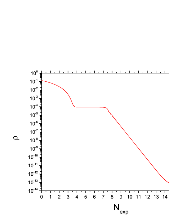
Figure 4: The evolution of the energy density $\rho$ as a function of $N_{\rm{exp}}$ for $n_{\rm s}=0.96$ and $\gamma=$ $0.25$ with an early inflationary stage.

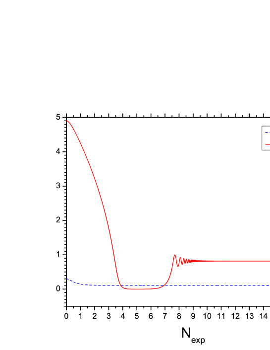
Figure 5: The evolution of the fields $\sigma$ and $\zeta$ as functions of $N_{\rm{exp}}$ for $n_{\rm s}=0.96$ and $\gamma=$ $0.25$ with an early inflationary stage.

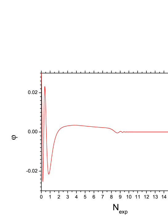
Figure 6: The evolution of the field $\varphi$ as a function of $N_{\rm{exp}}$ for $n_{\rm s}=0.96$ and $\gamma=$ $0.25$ with an early inflationary stage.

The field $\sigma$ drops to about $1/2$ its initial value during the first e-folding of expansion, to about $1/3$ during the second e-folding and it remains essentially frozen to a value well above $\sigma_{*}$ until the later inflation begins. The field $\varphi$ oscillates rapidly during the first stage of the early inflation with decreasing amplitude then remains more or less frozen during the second stage of the early inflation and starts oscillating again with decreasing amplitude after the end of the early inflation. Anologous behavior exhibit the fields $\bar{\varphi}_{1},\bar{\varphi}_{2}$.

We also provide initial conditions which lead to other scenarios of “observable” inflation with monotonic $V_{\rm{inf}}$. For $n_{\rm s}=0.95$ and $\gamma=0.25$ we have $\kappa\simeq 0.1104$, $\sigma_{*}\simeq 0.1238$ and initial field values $\zeta=4.54,\sigma=0.4,\varphi=\bar{\varphi}_{1}=\bar{\varphi}_{2}=0.03$. For $n_{\rm s}=0.96$ and $\gamma=0.30$ we have $\kappa\simeq 0.0841$, $\sigma_{*}\simeq 0.1035$ and initial field values $\zeta=4.75,\sigma=0.3,\varphi=\bar{\varphi}_{1}=\bar{\varphi}_{2}=0.026$. For $n_{\rm s}=0.97$ and $\gamma=0.25$ we have $\kappa\simeq 0.0216$, $\sigma_{*}\simeq 0.0314$ and initial field values $\zeta=4.95,\sigma=0.3,\varphi=0.08,\bar{\varphi}_{1}=\bar{\varphi}_{2}=0.07$. Finally, for $n_{\rm s}=0.97$ and $\gamma=0.45$ we have $\kappa\simeq 0.0492$, $\sigma_{*}\simeq 0.0686$ and initial field values $\zeta=4.85,\sigma=0.3,\varphi=\bar{\varphi}_{1}=\bar{\varphi}_{2}=0.037$.

In the case of a non-monotonic $V_{\rm{inf}}$ the choice of appropriate initial conditions becomes much more tricky because we must ensure that when $\rho\simeq\kappa^{2}M^{4}$ it holds that $|\sigma_{*}|<|\sigma|<|\sigma_{\rm{lmax}}|$ with $|\sigma_{\rm{lmax}}|$ being the value of $|\sigma|$ for which $V_{\rm{inf}}$ is a local maximum. In addition, when $\sigma=\sigma_{*}$ the time derivative of $\sigma$ should be close to the one predicted by the slow-roll approximation. It is obvious that the outcome is extremely sensitive to the initial field values. Moreover, we should be aware of the fact that quantum fluctuations during the early inflationary stage, which are not taken into account by our classical treatment, could play a crucial role.

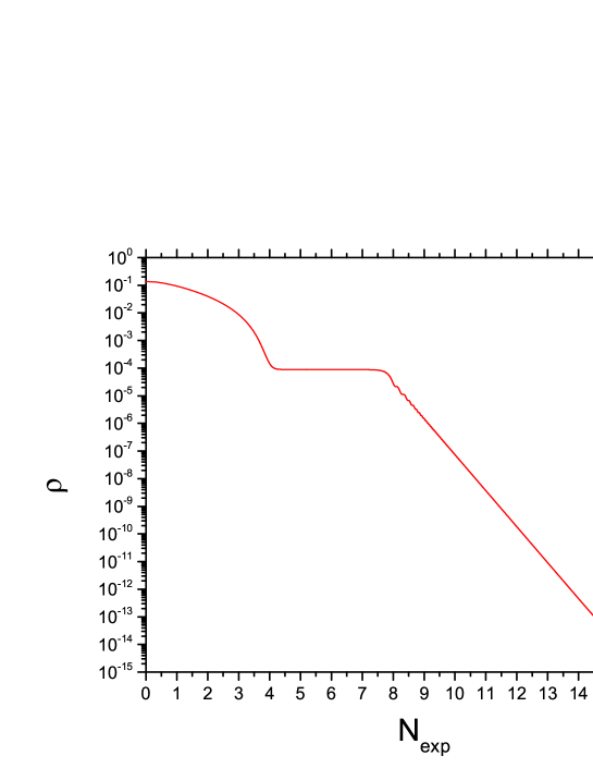
Figure 7: The evolution of the energy density $\rho$ as a function of $N_{\rm{exp}}$ in the scenario with $\beta=1/150$, $x_{*}=0.5$ and $\kappa=0.01$ (non-monotonic $V_{\rm{inf}}$) with an early inflationary stage.

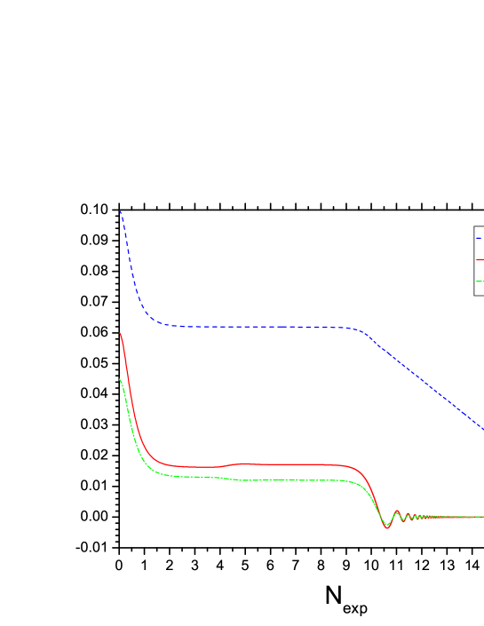
Figure 8: The evolution of the fields $\sigma$, $\varphi$, and $\bar{\varphi}_{1}$ as functions of $N_{\rm{exp}}$ in the scenario with $\beta=1/150$, $x_{*}=0.5$ and $\kappa=0.01$ (non-monotonic $V_{\rm{inf}}$) with an early inflationary stage.

Let us consider the scenario with non-monotonic $V_{\rm{inf}}$ having $\beta=1/150$, $x_{*}=0.5$ and $\kappa=0.01$ lps . For such a choice $n_{\rm s}\simeq 0.96$, $N_{*}\simeq 50$, $|\sigma_{*}|\simeq 0.01378$, $M\simeq 2.17\times 10^{-3}$, and $|\sigma_{\rm{lmax}}|\simeq 0.0197$. The initial field values are chosen to be $\zeta=5.15,\sigma=0.1,\varphi=0.06,\bar{\varphi}_{1}=\bar{\varphi}_{2}=0.045$ resulting in an initial energy density $\rho_{0}\simeq 0.1347$. In Fig. 7 we plot the energy density $\rho$ and in Fig. 8 the values of the fields $\sigma,\varphi$, and $\bar{\varphi}_{1}$ as functions of $N_{\rm{exp}}$. The required number of e-foldings of expansion in Eq. (41) with $\rho_{0}\simeq 0.1347$ and $\rho_{\rm{inf}}=3\kappa^{2}M^{4}\simeq 6.65\times 10^{-15}$ is $N_{\rm{req}}\simeq 15.32$ while the actual number is $N_{\rm{exp}}\simeq 15.54$. We conclude again that the early inflation is able to provide the necessary homogenization required in order to allow the onset of the later inflation. The fields $\sigma$, $\varphi$, $\bar{\varphi}_{1}$ (and also $\bar{\varphi}_{2}$) decrease sharply during the first e-folding and remain frozen until $N_{\rm{exp}}\simeq 10$. Then, $\varphi$, $\bar{\varphi}_{1}$ (and also $\bar{\varphi}_{2}$) perform damped oscillations with their amplitudes becoming soon very small while $\sigma$ suffers a gradual decrease in magnitude until the later inflation begins. When $\rho\simeq\kappa^{2}M^{4}\simeq 2.22\times 10^{-15}$ $\sigma$ is clearly below $\sigma_{\rm{lmax}}\simeq 0.0197$ and well above $\sigma_{*}\simeq 0.01378$ as required.

Comparing the cases of monotonic and non-monotonic inflationary potential we see that in the latter the initial ratio $|\sigma/\varphi|$ is considerably smaller. In the case of the non-monotonic potential, however, if the size of the initial value of the field $\varphi$ (and $\bar{\varphi}_{1}$, $\bar{\varphi}_{2}$) decreases somewhat, when the energy density falls to $\rho\simeq\kappa^{2}M^{4}\simeq 2.22\times 10^{-15}$ $\sigma$ remains well above $\sigma_{\rm{lmax}}\simeq 0.0197$ and eventually is trapped in the local minimum of the potential.

Our earlier discussion should have made clear that the problem of the initial conditions for inflation consists of two logically distinct components, namely the initial field values and the creation of a homogeneous region in space of appropriate size where the fields take these values. If we assume that this region already exists then it is possible to solve very simply the other part of the initial condition problem using the same “anomalous” D-term potential of Eq. (48) in which the $\xi$-term does not necessarily take the very specific value $\xi=1/3$ and the initial value of $|\zeta|$ is neither very large nor very small. We choose $\xi=0.5$ and $g=1$ in order to obtain initial energy density $\rho_{0}\sim 0.1$.

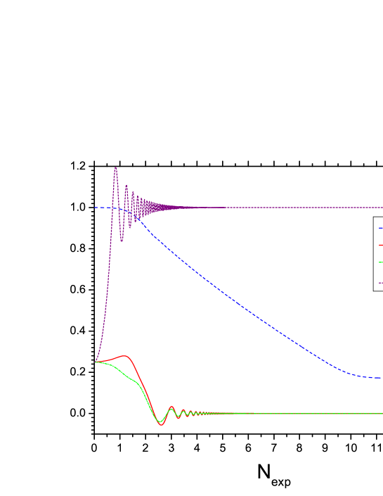
Figure 9: The evolution of the fields $\sigma$, $\varphi$, $\bar{\varphi}_{1}$, and $\zeta$ as functions of $N_{\rm{exp}}$ for $n_{\rm s}=0.96$ and $\gamma=0.25$ without an early inflationary stage.

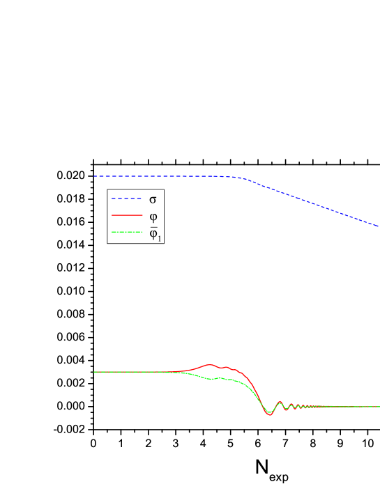
Figure 10: The evolution of the fields $\sigma$, $\varphi$, and $\bar{\varphi}_{1}$ as functions of $N_{\rm{exp}}$ in the scenario with $\beta=1/150$, $x_{*}=0.5$ and $\kappa=0.01$ (non-monotonic $V_{\rm{inf}}$) without an early inflationary stage.

As a demonstration let us consider the scenario of “observable” inflation with $n_{\rm s}=0.96$ and $\gamma=0.25$. Initially we set $\sigma=1$ and $\zeta=\varphi=\bar{\varphi}_{1}=\bar{\varphi}_{2}=0.25$ such that $\rho_{0}\simeq 0.1103$. In Fig. 9 we plot the evolution of the fields $\sigma$, $\varphi$, $\bar{\varphi}_{1}$, and $\zeta$ as functions of $N_{\rm{exp}}$. We see that $\zeta$ starts oscillating fast with decreasing amplitude around its minimum at $\zeta=\sqrt{2\xi}=1$ already from the first e-folding of expansion. Also $\varphi,\bar{\varphi}_{1}$ (and $\bar{\varphi}_{2}$) after the second e-folding perform fast dumped oscillations around zero and soon become very small in size. Finally, $\sigma$ after the first e-folding decreases continuously until the onset of inflation at $N_{\rm{exp}}\simeq 9.6$ reaching a value $\sigma\simeq 0.17$ considerably larger than $\sigma_{*}\simeq 0.07$.

We may also consider the scenario with non-monotonic $V_{\rm{inf}}$ having $\beta=1/150$, $x_{*}=0.5$ and $\kappa=0.01$. In this case we choose an initial value of $\sigma=0.02$ very close to the position of the local maximum of $V_{\rm{inf}}$ in order to minimize the sensitivity to the initial conditions. The initial values for the remaining fields are $\zeta=0.25$, and $\varphi=\bar{\varphi}_{1}=\bar{\varphi}_{2}=0.003\gg M^{2}$ leading to $\rho_{0}\simeq 0.1103$. The evolution of the fields $\sigma$, $\varphi$, and $\bar{\varphi}_{1}$ as functions of $N_{\rm{exp}}$ is presented in Fig. 10. We see that although the initial value of $\sigma$ is not much larger than $\sigma_{*}\simeq 0.01378$, $\sigma$ remains larger than $\sigma_{*}$ when inflation begins ($N_{\rm{exp}}\simeq 10.6$).

IV Summary

We investigated the possibility of having a viable scenario of SUSY hybrid inflation with scalar spectral index $n_{\rm s}\simeq 0.96-0.97$ and monotonic inflationary potential. This is achieved for values of the superpotential coupling $\kappa$ and the coefficient $\alpha$ of the first correction to the minimal Kähler potential involving the inflaton for which the quantity $\gamma$ in Eq. (12) lies in a certain interval. The lower endpoint of this interval is close to $0.25$ with the upper endpoint being an increasing function of $n_{\rm s}$.

We also provided a solution to the problem of the initial conditions leading to such inflationary scenarios which employs an additional early inflationary stage. This approach seems to be applicable to the case of a non-monotonic inflationary potential as well in the sense that it generates the necessary homogeneous region at the Planck scale where the fields are almost constant with values which are not unnaturally small in size. However, the extreme sensitivity to the choice of these initial field values justifies our preference for monotonic potentials.

References

(1)
G. Dvali, Q. Shafi, and R. Schaefer, Phys. Rev. Lett.
73, 1886 (1994).
(2)
E.J. Copeland, A.R. Liddle, D.H. Lyth, E.D. Stewart,
and D. Wands, Phys. Rev. D 49, 6410 (1994).
(3) C. Panagiotakopoulos, Phys. Lett. B 402, 257 (1997).
(4)
M. Bastero-Gil, S.F. King, and Q. Shafi, Phys. Lett.
B 651, 345 (2007).