Achievability Performance Bounds for Integer-Forcing Source Coding

Abstract

Integer-forcing source coding has been proposed as a low-complexity method for compression of distributed correlated Gaussian sources. In this scheme, each encoder quantizes its observation using the same fine lattice and reduces the result modulo a coarse lattice. Rather than directly recovering the individual quantized signals, the decoder first recovers a full-rank set of judiciously chosen integer linear combinations of the quantized signals, and then inverts it. It has been observed that the method works very well for “most” but not all source covariance matrices. The present work quantifies the measure of bad covariance matrices by studying the probability that integer-forcing source coding fails as a function of the allocated rate, where the probability is with respect to a random orthonormal transformation that is applied to the sources prior to quantization. For the important case where the signals to be compressed correspond to the antenna inputs of relays in an i.i.d. Rayleigh fading environment, this orthonormal transformation can be viewed as being performed by nature. The scheme is also studied in the context of a non-distributed system. Here, the goal is to arrive at a universal, yet practical, compression method using equal-rate quantizers with provable performance guarantees. The scheme is universal in the sense that the covariance matrix need only be learned at the decoder but not at the encoder. The goal is accomplished by replacing the random orthonormal transformation by transformations corresponding to number-theoretic space-time codes.

I Introduction

Integer-forcing (IF) source coding, proposed in [1], is a scheme for distributed lossy compression of correlated Gaussian sources under a minimum mean squared error distortion measure. Similar to its channel coding counterpart, in this scheme, all encoders use the same nested lattice codebook. Each encoder quantizes its observation using the fine lattice as a quantizer and reduces the result modulo the coarse lattice, which plays the role of binning. Rather than directly recovering the individual quantized signals, the decoder first recovers a full-rank set of judiciously chosen integer linear combinations of the quantized signals, and then inverts it. An appealing feature of integer-forcing source coding, not shared by previously proposed practical methods (e.g., Wyner-Ziv coding) for the distributed source coding problem, is its inherent symmetry, supporting equal distortion and quantization rates. A potential application of IF source coding is to distributed compression of signals received at several relays as suggested in [1] and further explored in [2].

Similar to IF channel coding, IF source coding works well for “most” but not all Gaussian vector sources. Following the approach of [3], in the present work we quantify the measure of bad source covariance matrices by considering a randomized version of IF source coding where a random orthogonal transformation is applied to the sources prior to quantization. Specifically, we derive bounds on the worst-case (with respect to a compound class of Gaussian sources) outage probability when the precoding matrices are drawn from the circular real ensemble (CRE); that is, they are uniformly distributed with respect to the Haar measure. While in general such a transformation implies joint processing at the encoders, we note that in some natural scenarios, including that of distributed compression of signals received at relays in an i.i.d. Rayleigh fading environment, the random transformation is actually performed by nature. In fact, it was already empirically observed in [1] that IF source coding performs very well in the latter scenario.

We then consider the performance of IF source coding when used in conjunction with judiciously chosen (deterministic) unitary precoding. Such precoding requires joint processing of the different sources prior to quantization and is thus precluded in a distributed setting. Nonetheless, the scheme has an important advantage with respect to traditional centralized source coding of correlated sources. Whereas the traditional approach requires utilizing the statistical characterization of the source at the encoder side, e.g., via the application of appropriate transform coding, the considered compression scheme, in contrast, applies a universal transformation, i.e., a transformation that is independent of the source statistics. Furthermore, no bit loading is needed. That is, the components of the output of the transformation are all quantized at the same rate and hence the operation of the encoder does not depend on the source statistics. This characteristic may be advantageous in scenarios where the complexity of the encoder should be kept to a minimum whereas larger computational resources are available in the reconstruction stage where of course knowledge of the statistics of the source has to be obtained and utilized in some manner. We refer the reader to [5] which describes a practical method by which the decoder may estimate the statistics of the source from the modulo-reduced quantized samples, whereas the encoder may remain oblivious to the source statistics.

For such a centralized application of IF source coding, we are able to derive stronger performance guarantees than those we derive for the distributed setting. Namely, in the centralized setting, we show that by employing transformations derived from algebraic number-theoretic constructions, successful source reconstruction can be guaranteed for any Gaussian source in the considered compound class. Thus, we need not allow for outage events. For general Gaussian sources, such guarantees require performing precoding jointly over space and time. In contrast, for the case of parallel (independent) Gaussian sources with different variances, space-only precoding suffices. This distinction closely mirrors the well-known results concerning transformations for achieving maximal diversity for communication over fading channels, as described in [6].

The rest of this paper is organized as follows. Section II formulates the problem of distributed compression of Gaussian sources in a compound vector source setting and provides some relevant background on IF source coding. Section III describes randomly precoded IF source coding and its empirical performance. Section IV derives upper bounds on the probability of failure of randomly-precoded IF as a function of the excess rate. In Section V, deterministic linear precoding is considered. A bound on the worst-case necessary excess rate is derived for any number of sources with any correlation matrix when space-time precoding derived from non-vanishing determinant codes is used. Further, we show that this bound can be significantly tightened for the case of uncorrelated sources.

II Problem Formulation and Background

In this section we provide the problem formulation and briefly recall the achievable rates of IF source coding as developed in [1]. We refer the reader to the latter for an introduction and overview of IF source coding.

II-A Distributed Compression of Gaussian Sources

We start by recalling the classical problem of distributed lossy compression of jointly Gaussian real random variables under a quadratic distortion measure. Specifically, we consider a distributed source coding setting with $K$ encoding terminals and one decoder. Each of the $K$ encoders has access to a vector of $n$ i.i.d. realizations of the random variable $x_{k}$, $k=1,...,K$. The random vector ${\bf x}=(x_{1},\ldots,x_{K})^{T}$ (corresponding to the different sources) is assumed to be Gaussian with zero mean and covariance matrix $\mathbf{K}_{\bf xx}\triangleq\mathbb{E}\left(\bf{x}\bf{x}^{T}\right)$.

Each encoder maps its observation $\bf{x}_{k}$ to an index using the encoding function

$$\mathcal{E}_{k}~{}:~{}\mathbb{R}^{n}\rightarrow\left\{1,...,2^{nR_{k}}\right\},$$ (1)

and sends the index to the decoder.

The decoder is equipped with $K$ decoding functions

$$\mathcal{D}_{k}~{}:~{}\left\{1,...,2^{nR_{1}}\right\}\times\cdots\times\left\{1,...,2^{nR_{K}}\right\}\rightarrow\mathbb{R}^{n},$$ (2)

where $k=1,...,K$. Upon receiving $K$ indices, one from each terminal, it generates the estimates

$$\hat{\bf{x}}_{k}=\mathcal{D}_{k}\left(\mathcal{E}_{1}({\bf x}_{1}),...,\mathcal{E}_{K}({\bf x}_{K})\right),~{}~{}k=1,...,K.$$ (3)

A rate-distortion vector $(R_{1},...,R_{K};d_{1},...,d_{K})$ is achievable if there exist encoding functions, $\mathcal{E}_{1},...,\mathcal{E}_{K}$, and decoding functions, $\mathcal{D}_{1},...,\mathcal{D}_{K}$, such that $\frac{1}{n}\mathbb{E}\left(\|{\bf x}_{k}-\hat{\bf x}_{k}\|^{2}\right)\leq d_{k}$, for all $k=1,...,K$.

We focus on the symmetric case where $d_{1}=\cdots=d_{K}=d$ and $R_{1}=\cdots=R_{K}=R/K$ where we denote the sum rate by $R$. The best known achievable scheme (for this symmetric setting; see [1], Section I) is that of Berger and Tung [7], for which the following (in general, suboptimal) sum rate is achievable

$$\sum_{k=1}^{K}R_{k} \geq\frac{1}{2}\log\det{\left(\mathbf{I}+\frac{1}{d}\mathbf{K}_{\bf xx}\right)}$$

$$\triangleq R_{\rm BT}.$$ (4)

As shown in [1], $R_{\rm BT}$ is a lower bound on the achievable rate of IF source coding. We will refer to $R_{\rm BT}$ as the Berger-Tung benchmark. To simplify notation, we note that $d$ can be “absorbed” into $\mathbf{K}_{\bf xx}$. Hence, without loss of generality, we assume throughout that $d=1$.

II-B Compound Source Model And Scheme Outage Formulation

Consider distributed lossy compression of a vector of Gaussian sources

$$\mathbf{x}\sim\mathcal{N}(0,\mathbf{K}_{\bf xx}).$$ (5)

We define the following compound class of Gaussian sources, having the same value of $R_{\rm BT}$, via their covariance matrix:

$$\mathcal{K}(R_{\rm BT})=\left\{\mathbf{K}_{\bf xx}\in\mathbb{R}^{K\times K}:\frac{1}{2}\log\det\left(\mathbf{I}+\mathbf{K}_{\bf xx}\right)=R_{\rm BT}\right\}.$$ (6)

We quantify the measure of the set of source covariance matrices by considering outage events, i.e., those events (sources) where integer forcing fails to achieve the desired level of distortion even though the rate exceeds $R_{\rm BT}$. More broadly, for a given quantization scheme, denote the necessary rate to achieve $d=1$ for a given covariance matrix $\mathbf{K_{xx}}$ as $R_{\rm scheme}(\mathbf{K_{xx}})$. Then, given a target rate $R>R_{\rm BT}$ and a covariance matrix $\mathbf{K_{xx}}\in\mathcal{K}(R_{\rm BT})$, a scheme outage occurs when $R_{\rm scheme}(\mathbf{K_{xx}})>R$.

To quantify the measure of “bad” covariance matrices, we follow [3] and apply a random orthonormal precoding matrix to the (vector of) source samples prior to encoding. As mentioned above, this amounts to joint processing of the samples and hence the problem is no longer distributed in general. Nonetheless, as in the scenario described in Section IV-A, in certain statistical settings, this precoding operation is redundant as it can be viewed as being performed by nature.

Applying a precoding matrix to the source vector, we obtain a transformed source vector

$$\tilde{\bf x}=\mathbf{P}{\bf x},$$ (7)

with covariance matrix

$$\mathbf{K}_{\tilde{x}\tilde{x}} =\mathbf{P}\mathbf{K}_{\bf xx}\mathbf{P}^{T}.$$ (8)

It follows that the achievable rate of a quantization scheme for the precoded source is $R_{\rm scheme}(\mathbf{K}_{\tilde{\bf x}\tilde{\bf x}})$. When $\mathbf{P}$ is drawn at random, the latter rate is also random. The worst-case (WC) scheme outage probability is defined in turn as

$$P^{\rm WC}_{\rm out,scheme}\left(R_{\rm BT},\Delta R\right)$$

$$=\sup_{\mathbf{K}_{\bf xx}\in\mathcal{K}(R_{\rm BT})}{\rm Pr}\left(R_{\rm scheme}(\mathbf{K}_{\tilde{\bf x}\tilde{\bf x}})>R_{\rm BT}+\Delta R\right),$$ (9)

where the probability is over the ensemble of precoding matrices considered and $\Delta R$ is the gap to the Berger-Tung benchmark.

In the sequel, we quantify the tradeoff between the quantization rate $R$ (or equivalently, between the excess rate $\Delta R=R-R_{\rm BT}$) and the outage probability $P^{\rm WC}_{\rm out,IF}\left(R_{\rm BT},\Delta R\right)$ as defined in (9).

II-C Integer-Forcing Source Coding

In a manner similar to IF equalization for channel coding, IF can be applied to the problem of distributed lossy compression. The approach is based on standard quantization followed by lattice-based binning. However, in the IF framework, the decoder first uses the bin indices for recovering linear combinations with integer coefficients of the quantized signals, and only then recovers the quantized signals themselves.

For our purposes, it suffices to state only the achievable sum rate of IF source coding. We refer the reader to [1] for the derivation and proofs.

Theorem 1 ( [1], Theorem 1).

For any distortion $d>0$ and any full-rank integer matrix $\mathbf{A}=[{\bf a}_{1}\cdots{\bf a}_{K}]^{T}\in\mathbb{Z}^{K\times K}$, there exists a (sequence of) nested lattice pair(s) $\Lambda\in\Lambda_{f}$ such that IF source coding can achieve any sum rate satisfying

$$R>R_{\rm IF}(\mathbf{K}_{\bf xx},d;\mathbf{A})\triangleq\frac{K}{2}\log\left(\max_{k=1,\ldots,K}{\bf a}_{k}^{T}\left(\mathbf{I}+\frac{1}{d}\mathbf{K}_{\bf xx}\right){\bf a}_{k}\right)$$ (10)

We further note that this sum rate is achieved via symmetric rate allocation, i.e., by allocating $R_{k}=R_{\rm IF}(\mathbf{K}_{\bf xx},d;\mathbf{A})/K$ bits to each of the $K$ encoders. Since we assume $d=1$, it follows that IF source coding can achieve any (sum) rate satisfying

$$R >R_{\rm IF}^{\rm opt}(\mathbf{K}_{\bf xx})$$

$$\triangleq R_{\rm IF}(\mathbf{K}_{\bf xx};\mathbf{A}^{\rm opt})$$

$$=\frac{K}{2}\log\left(\min_{\begin{subarray}{c}\mathbf{A}\in\mathbb{Z}^{K\times K}\\ \det{\mathbf{A}}\neq 0\end{subarray}}\max_{k=1,...,K}{\bf a}_{k}^{T}\left(\mathbf{I}+\mathbf{K}_{\bf xx}\right){\bf a}_{k}\right),$$ (11)

where $\mathbf{a}_{k}^{T}$ is the $k$th row of the integer matrix $\mathbf{A}$.

The matrix $\mathbf{I}+\mathbf{K}_{\bf xx}$ is symmetric and positive definite, and therefore it admits a Cholesky decomposition

$$\mathbf{I}+\mathbf{K}_{\bf xx}=\mathbf{F}\mathbf{F}^{T}.$$ (12)

With this notation, we have

$$R_{\rm IF}^{\rm opt}(\mathbf{K}_{\bf xx})=\frac{K}{2}\log\left(\min_{\begin{subarray}{c}\mathbf{A}\in\mathbb{Z}^{K\times K}\\ \det{\mathbf{A}}\neq 0\end{subarray}}\max_{k=1,...,K}\|\mathbf{F}^{T}\bf{a}_{k}\|^{2}\right).$$ (13)

Denote by $\Lambda(\mathbf{F}^{T})$ the $K$-dimensional lattice spanned by the matrix $\mathbf{F}^{T}$, i.e.,

$$\Lambda(\mathbf{F}^{T})\triangleq\left\{\mathbf{F}^{T}\bf{a}:~{}a\in\mathbb{Z}^{K}\right\}.$$ (14)

Then the problem of finding the optimal matrix $\mathbf{A}$ is equivalent to finding the shortest set of $K$ linearly independent vectors in $\Lambda(\mathbf{F}^{T})$. In other words, the rate per encoder achieved by IF source coding can be expressed using the $k$th successive minimum of the lattice $\Lambda(\mathbf{F}^{T})$, where we recall that in general, for a full-rank $K\times K$ matrix $\mathbf{G}$:

Definition 1.

(successive minima) Let $\Lambda(\mathbf{G})$ be a lattice spanned by the full-rank matrix $\mathbf{G}\in\mathbb{R}^{K\times K}$. For $k=1,...,K$, we define the $k$’th successive minimum as

$$\lambda_{k}(\mathbf{G})\triangleq\inf\left\{r:{\rm dim}\left({\rm span}\left(\Lambda(\mathbf{G})\cap\mathcal{B}_{K}(r)\right)\right)\geq k\right\}$$ (15)

where $\mathcal{B}_{K}(r)=\left\{{\bf x}\in\mathbb{R}^{K}:\|{\bf x}\|\leq r\right\}$ is the closed ball of radius $r$ around ${\bf 0}$. In words, the $k$-th successive minimum of a lattice is the minimal radius of a ball centered around ${\bf 0}$ that contains $k$ linearly independent lattice points.

Thus, (13) can be restated as saying that IF source coding can achieve any rate greater than

$$R_{\rm IF}^{\rm opt}(\mathbf{K}_{\bf xx}) =\frac{K}{2}\log\left(\lambda_{K}^{2}(\mathbf{F}^{T})\right).$$ (16)

Just as successive interference cancellation significantly improves the achievable rate of IF equalization in channel coding (see, e.g., [8]), an analogous scheme can be implemented in the case of IF source coding. Specifically, for a given full-rank integer matrix $\mathbf{A}$, let $\mathbf{L}$ be defined by the Cholesky decomposition

$$\mathbf{A}\left(\mathbf{I}+\mathbf{K}_{\bf xx}\right)\mathbf{A}^{T}=\mathbf{L}\mathbf{L}^{T}$$ (17)

and denote the $m$th element of the diagonal of $\mathbf{L}$ by $\ell_{m,m}$. Then, as shown in [9] and [10], the achievable rate of successive IF source coding (which we denote as IF-SUC) for this choice of $\mathbf{A}$ is given by

$$R_{\rm IF-SUC}(\mathbf{K}_{\bf xx};\mathbf{A})=K\cdot\max_{k=1,\ldots,K}R_{{\rm IF-SUC},k}(\mathbf{K}_{\bf xx};\mathbf{A}),$$ (18)

where

$$R_{{\rm IF-SUC},k}(\mathbf{K}_{\bf xx};\mathbf{A})=\frac{1}{2}\log\left(\ell_{k,k}^{2}\right).$$ (19)

We refer the reader to pages 36-37 in [9] for details. Finally, by optimizing over the choice of $\mathbf{A}$, we obtain

$$R_{{\rm IF-SUC}}^{\rm opt}(\mathbf{K}_{\bf xx}) \triangleq R_{{\rm IF-SUC}}(\mathbf{K}_{\bf xx};\mathbf{A}^{\rm opt}_{\rm SUC})$$

$$=\min_{\begin{subarray}{c}\mathbf{A}\in\mathbb{Z}^{K\times K}\\ \det{\mathbf{A}}\neq 0\end{subarray}}R_{\rm IF-SUC}(\mathbf{K}_{\bf xx};\mathbf{A}).$$ (20)

While the gap between $R_{\rm IF}$ (and even more so $R_{\rm IF-SUC}$) and $R_{\rm BT}$ is quite small for most covariance matrices, it can nevertheless be arbitrarily large. We next quantify the measure of bad covariance matrices by considering randomly-precoded IF source coding.

III CRE-Precoded IF Source Coding and its Empirical Performance

Recalling (11), and with a slight abuse of notation, the rate of IF source coding for a given precoding matrix $\mathbf{P}$ is denoted by

$$R_{\rm IF}^{\rm opt}(\mathbf{K}_{\bf xx},\mathbf{P})\triangleq R_{\rm IF}^{\rm opt}(\mathbf{P}\mathbf{K}_{\bf xx}\mathbf{P}^{T})$$

$$=\frac{K}{2}\log\left(\min_{\begin{subarray}{c}\mathbf{A}\in\mathbb{Z}^{K\times K}\\ \det{\mathbf{A}}\neq 0\end{subarray}}\max_{k=1,...,K}{\bf a}_{k}^{T}\left(\mathbf{I}+\mathbf{P}\mathbf{K}_{\bf xx}\mathbf{P}^{T}\right){\bf a}_{k}\right).$$ (21)

Since $\mathbf{K_{\bf xx}}$ is symmetric, it allows orthonormal diagonalization

$$\mathbf{I}+\mathbf{K_{\bf xx}}=\mathbf{U}\mathbf{D}\mathbf{U}^{T}.$$ (22)

When unitary precoding is applied, we have

$$\mathbf{I}+\mathbf{P}\mathbf{K_{xx}}\mathbf{P}^{T}=\mathbf{P}\mathbf{U}\mathbf{D}\mathbf{U}^{T}\mathbf{P}^{T}.$$ (23)

To quantify the measure of “bad” sources, we consider precoding matrices that are uniformly (Haar) distributed over the group of orthonormal matrices. Such a matrix ensemble is referred to as CRE and is defined by the unique distribution on orthonormal matrices that is invariant under left and right orthonornal transformations [11]. That is, given a random matrix $\mathbf{P}$ drawn from the CRE, for any orthonormal matrix $\grave{\mathbf{U}}$, both ${\mathbf{P}}\grave{\mathbf{U}}$ and $\grave{\mathbf{U}}{\mathbf{P}}$ are equal in distribution to ${\mathbf{P}}$. Since $\mathbf{P}\mathbf{U}^{T}$ is equal in distribution to ${\mathbf{P}}$ for CRE precoding, for the sake of computing outage probabilities, we may simply assume that $\mathbf{U}^{T}$ (and also $\mathbf{U}$) is drawn from the CRE.

For a specific choice of integer vector ${\bf a_{k}}$, we define (again, with a slight abuse of notation)

$$R_{\rm IF}(\mathbf{D},\mathbf{U};{\bf a}_{k}) \triangleq\frac{1}{2}\log\left({\bf a}_{k}^{T}\mathbf{U}\mathbf{D}\mathbf{U}^{T}{\bf a}_{k}\right)$$

$$=\frac{1}{2}\log\left(\|\mathbf{D}^{1/2}\mathbf{U}^{T}{\bf a}_{k}\|^{2}\right),$$ (24)

and correspondingly

$$R_{\rm IF}^{\rm opt}(\mathbf{D},\mathbf{U})\triangleq$$

$$\frac{K}{2}\log\left(\min_{\begin{subarray}{c}\mathbf{A}\in\mathbb{Z}^{K\times K}\\ \det{\mathbf{A}}\neq 0\end{subarray}}\max_{k=1,...,K}\|\mathbf{D}^{1/2}\mathbf{U}^{T}{\bf a}_{k}\|^{2}\right).$$ (25)

Let $\Lambda$ be the lattice spanned by $\mathbf{G}=\mathbf{D}^{1/2}\mathbf{U}^{T}$. Then (25) may be rewritten as

$$R_{\rm IF}^{\rm opt}(\mathbf{D},\mathbf{U})=\frac{K}{2}\log\left(\lambda_{K}^{2}(\Lambda)\right).$$ (26)

Let us denote the set of all diagonal matrices having the same value of $R_{\rm BT}$, i.e.,

$$\mathbb{D}(R_{\rm BT},K)=\{\mathbf{D}~{}:~{}\det\left(\mathbf{D}\right)=2^{2R_{\rm BT}}\}.$$ (27)

We may thus rewrite the worst-case outage probability of IF source coding, defined in (9), as

$$P^{\rm WC}_{\rm out,IF}\left(R_{\rm BT},\Delta R\right)$$

$$=\sup_{\mathbf{D}\in\mathbb{D}(R_{\rm BT},K)}{\rm Pr}\left(R_{\rm IF}^{\rm opt}(\mathbf{D},\mathbf{U})>R_{\rm BT}+\Delta R\right),$$ (28)

where the probability is with respect to the random selection of $\mathbf{U}$ that is drawn from the CRE.

To illustrate the worst-case performance of CRE-precoded IF, we present its empirical performance for the case of a two-dimensional compound Gaussian source vector, where the outage probability (28) is computed via Monte-Carlo simulation.

Figure 1 depicts the results for different values of $R_{\rm BT}$. Rather than plotting the worst-case outage probability, its complement is depicted, i.e., we plot the probability that the rate of IF falls below $R_{\rm BT}+\Delta R$. As can be seen from the figure, the WC outage probability (as a function of $\Delta R$) converges to a limiting curve as $R_{\rm BT}$ increases.

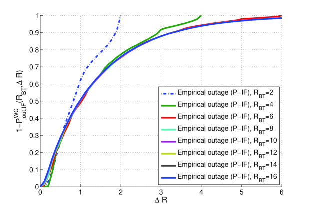
Figure 1: Empirical results for (the complement of) the worst-case outage probability of IF source coding when applied to a two-dimensional compound Gaussian source vector as a function of $\Delta R$, for various values of $R_{\rm BT}$.

Figure 2 depicts the results for the single (high) rate $R_{\rm BT}=16$. The required compression rate required to support a given worst-case outage probability constraint is marked, for several outage probabilities. We observe that:

• For $10\%$ worst-case outage probability, a gap of $\Delta R=3.292$ bits (or $1.646$ bits per source) is required.

• For $5\%$ worst-case outage probability, a gap of $\Delta R=4.293$ bits (or $2.1465$ bits per source) is required.

• For $1\%$ worst-case outage probability, a gap of $\Delta R=6.665$ bits (or $3.3325$ bits per source) is required.

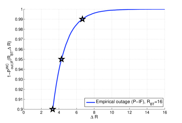
Figure 2: Zoom in on the empirical worst-case outage probability for a two-dimensional compound Gaussian source vector with $R_{\rm BT}=16$.

IV Upper Bounds on the Outage Probability for CRE-Precoded Integer-Forcing Source Coding

In this section we develop achievability bounds for randomly-precoded IF source coding. As the derivation is very much along the lines of the results for the analogous problem in channel coding as developed in [3], we refer to results from the latter in many points.

The next lemma provides an upper bound on the outage probability of precoded IF source coding as a function of $R_{\rm BT}$ and the rate gap $\Delta R$ (as well as the number of sources and $d_{\max}$ defined below). Denote

$$\mathbb{A}({\beta},\delta,K)=\left\{{\bf a}\in\mathbb{Z}^{K}:0<\|{\bf a}\|<\sqrt{\frac{{\beta}}{\delta}}\right\}.$$ (29)

Lemma 1.

For any $K$ Gaussian sources such that $\mathbf{D}\in\mathbb{D}(R_{\rm BT},K)$, and for $\mathbf{U}$ drawn from the CRE, we have

$${\rm Pr}\left(R_{\rm IF}^{\rm opt}(\mathbf{D},\mathbf{U})<R_{\rm BT}+\Delta R\right)$$

$$\leq\sum_{{\bf a}\in\mathbb{A}({\beta},1/d_{\max},K)}\frac{K\alpha(K)^{\frac{K-1}{2}}2^{-\frac{K-1}{K}(R_{\rm BT}+\Delta R)}}{\frac{\|{\bf a}\|^{K-1}}{2^{R_{\rm BT}}}{\sqrt{d_{\max}}}}$$ (30)

where $\displaystyle{d_{\max}=\max_{i}\mathbf{D}_{i,i}}$, the set ${\mathbb{A}({\beta},1/d_{\max},K)}$ is defined in (29), and where $\alpha(K)$ is defined in (35) below.

Proof.

Let $\Lambda^{*}$ denote the dual lattice of $\Lambda$ and note that it is spanned by the matrix

$$(\mathbf{G}^{T})^{-1}=\mathbf{D}^{-1/2}\mathbf{U}^{T}.$$ (31)

The successive minima of $\Lambda$ and $\Lambda^{*}$ are related by (Theorem 2.4 in [12])

$$\lambda_{1}(\Lambda^{*})^{2}\lambda_{K}(\Lambda)^{2}\leq\frac{K+3}{4}{\bar{\gamma}_{K}}^{2},$$ (32)

where

$$\bar{\gamma}_{K}=\max\{\gamma_{i}:1\leq i\leq K\}$$ (33)

with $\gamma_{K}$ denoting Hermite’s constant.

The tightest known bound for Hermite’s constant, as derived in [13], is

$$\gamma_{K}\leq\left(\frac{2}{\pi}\right)\Gamma\left(2+\frac{K}{2}\right)^{2/K}.$$ (34)

Since this is an increasing function of $K$, it follows that $\bar{\gamma}_{K}$ is smaller than the r.h.s. of (34). Combining the latter with the exact values of the Hermite constant for dimensions for which it is known, we define

$$\alpha(K)=\begin{cases}\frac{K+3}{4}\gamma_{K}^{2},&K=1-8,24\\ \frac{K+3}{4}\frac{2}{\pi}\Gamma\left(2+\frac{K}{2}\right)^{2/K},&{\rm otherwise}\end{cases}.$$ (35)

Therefore, we may bound the achievable rates of IF via the dual lattice as follows

$$R_{\rm IF}^{\rm opt}(\mathbf{D},\mathbf{U}) \leq\frac{K}{2}\log\left({\alpha(K)}\frac{1}{\lambda_{1}(\Lambda^{*})^{2}}\right).$$ (36)

Hence, we have

$${\rm Pr}\left(R_{\rm IF}^{\rm opt}(\mathbf{D},\mathbf{U})>R_{\rm BT}+\Delta R\right)$$

$$\leq{\rm Pr}\left(\frac{K}{2}\log\left(\alpha(K)\frac{1}{\lambda_{1}(\Lambda^{*})^{2}}\right)>R_{\rm BT}+\Delta R\right)$$

$$={\rm Pr}\left(\lambda_{1}(\Lambda^{*})^{2}<\alpha(K)2^{-\frac{2}{K}(R_{\rm BT}+\Delta R)}\right).$$ (37)

Denote

$${\beta}=\alpha(K)2^{-\frac{2}{K}(R_{\rm BT}+\Delta R)}.$$ (38)

We wish to bound (37), or equivalently, we wish to bound

$${\rm Pr}\left(\lambda_{1}^{2}(\Lambda^{*})<{{\beta}}\right)={\rm Pr}\left(\lambda_{1}(\Lambda^{*})<\sqrt{{\beta}}\right)$$ (39)

for a given matrix $\mathbf{D}\in\mathbb{D}(R_{\rm BT},K)$. Note that the event $\lambda_{1}(\Lambda^{*})<\sqrt{{\beta}}$ is equivalent to the event

$$\bigcup_{{\bf a}\in{\mathbb{Z}^{K}\setminus\{{\bf 0}\}}}||\mathbf{D}^{-1/2}\mathbf{U}^{T}\bf{a}||<\sqrt{{\beta}}.$$ (40)

Applying the union bound yields

$${\rm Pr}\left(\lambda_{1}(\Lambda^{*})<\sqrt{{\beta}}\right)\leq\sum_{{\bf a}\in\mathbb{Z}^{K}\setminus\{{\bf 0}\}}{\rm Pr}\left(||\mathbf{D}^{-1/2}\mathbf{U}^{T}{\bf a}||<\sqrt{{\beta}}\right).$$ (41)

Note that whenever $\frac{||{\bf a}||}{\sqrt{d_{\max}}}\geq\sqrt{{\beta}}$, we have

$${\rm Pr}\left(||\mathbf{D}^{-1/2}\mathbf{U}^{T}{\bf a}||<\sqrt{{\beta}}\right)=0.$$ (42)

Therefore, substituting $1/d_{\max}$ in (29), the set of relevant vectors ${\bf a}$ is

$${\mathbb{A}({\beta},1/d_{\max},K)}=\left\{{\bf a}\in\mathbb{Z}^{K}:0<||{\bf a}||<\sqrt{{\beta}d_{\max}}\right\}.$$ (43)

It follows from (41) and (42) that

$${\rm Pr}\left(\lambda_{1}(\Lambda^{*})<\sqrt{{\beta}}\right)\leq\sum_{{\bf a}\in{\mathbb{A}({\beta},1/d_{\max},K)}}{\rm Pr}\left(\|\mathbf{D}^{-1/2}\mathbf{U}^{T}{\bf a}\|<\sqrt{{\beta}}\right).$$ (44)

The rest of the proof follows the footsteps of Lemma 2 in [3] and is given in Appendix A. ∎

While Lemma 1 provides an explicit bound on the outage probability, in order to calculate it, one needs to go over all diagonal matrices in $\mathbb{D}(R_{\rm BT},K)$ and for each such diagonal matrix, sum over all the relevant integer vectors in $\mathbb{A}({\beta},1/d_{\max},K)$. Hence, the bound can be evaluated only for moderate compression rates and for a small number of sources. The following theorem, that may be viewed as the counterpart of Theorem 1 in [3], provides a looser, yet very simple closed-form bound. Another advantage for this bound is that it does not depend on the Berger-Tung achievable rate.

Theorem 2.

For any $K$ sources such that $\mathbf{D}\in\mathbb{D}(R_{\rm BT},K)$, and for $\mathbf{U}$ drawn from the CRE we have

$${\rm Pr}\left(R_{\rm IF}^{\rm opt}(\mathbf{D},\mathbf{U})>R_{\rm BT}+\Delta R\right)\leq c(K)2^{-\Delta R},$$ (45)

where

$$c(K)=K\alpha(K)^{\frac{K}{2}}(K+c_{\max})\frac{\pi^{K/2}}{\Gamma(K/2+1)},$$ (46)

$$\alpha(K)=\frac{K+3}{4}\frac{2}{\pi}\Gamma\left(2+\frac{K}{2}\right)^{2/K}$$ (47)

and

$$c_{\max}=\begin{cases}\left(2+\frac{\sqrt{K}}{2}\right)^{K}-\left(1-\frac{\sqrt{K}}{2}\right)^{K}&1\leq K<4\\ \left(1+\sqrt{K}\right)^{K}&K\geq 4\end{cases}.$$ (48)

Note that $c(K)$ is a constant that depends only on the number of sources $K$.

Proof.

See Appendix B. ∎

Similarly to the case of IF channel coding (cf., Section IV-C in [3]), analyzing Theorem 2 reveals that there are two main sources for looseness that may be further tightened:

• Union bound - While there is an inherent loss in the union bound, in fact, some terms in the summation (44) may be completely dropped. Specifically, using Corollary 1 in [3], the set $\mathbb{A}({\beta},1/d_{\max},K)$ appearing in the summation in (1) may be replaced by the smaller set $\mathbb{B}({\beta},1/d_{\max},K)$ where

$$\mathbb{B}({\beta},d,K)=$$

$$\left\{{\bf a}\in\mathbb{Z}^{K}:0<\|{\bf a}\|<\sqrt{\frac{{\beta}}{d}}\>{\rm and}\>\nexists 0<c<1\>{\rm s.t.}\>c{\bf a}\in\mathbb{Z}^{K}\right\}.$$ (49)

• Dual Lattice - Bounding via the dual lattice induces a loss reflected in (32). This may be circumvented for the case of a two-dimensional source vector by using IF-SUC, as accomplished in Lemma 2 and Theorem 3 which we present next.

Lemma 2.

For a two-dimensional Gaussian source vector such that $\mathbf{D}\in\mathbb{D}(R_{\rm BT},K)$, and for $\mathbf{U}$ drawn from the CRE, we have

$${\rm Pr}\left(R_{\rm IF-SUC}^{\rm opt}(\mathbf{D},\mathbf{U})>R_{\rm BT}+\Delta R\right)$$

$$\leq\sum_{{\bf a}\in\mathbb{B}({\beta},d_{\min},K)}\frac{2\sqrt{{\beta}}}{\|{\bf a}\|2^{R_{\rm BT}}\frac{1}{\sqrt{d_{\min}}}}$$ (50)

where $\displaystyle{d_{\min}=\min_{i}\mathbf{D}_{i,i}}$ and ${\mathbb{A}({\beta},d_{\min},K)}$ is defined in (29),

Proof.

See Appendix C. ∎

Theorem 3.

For a two-dimensional Gaussian source vector such that $\mathbf{D}\in\mathbb{D}(R_{\rm BT},K)$, and for $\mathbf{U}$ drawn from the CRE, we have

$${\rm Pr}\left(R_{\rm IF-SUC}^{\rm opt}(\mathbf{D},\mathbf{U})>R_{\rm BT}+\Delta R\right)\leq c^{\prime}(K)2^{-\Delta R},$$ (51)

where

$$c^{\prime}(K)=2\pi\left(5+3\sqrt{2}\right).$$ (52)

Proof.

See Appendix C. ∎

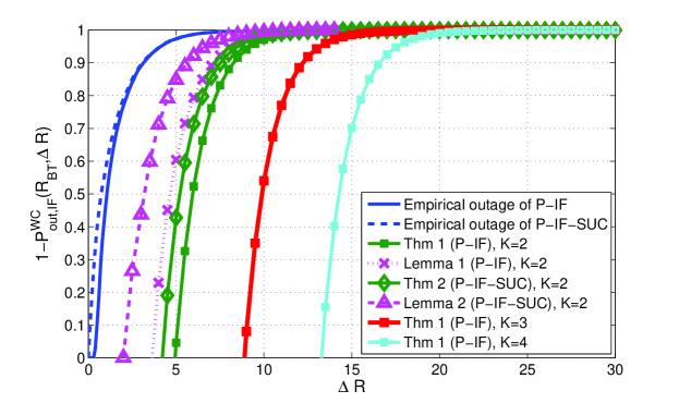
Figure 3: Upper bounds on the outage probability of IF source coding for various values of source dimension $K$.

Figure 3 depicts the bounds derived as well as results of a Monte Carlo evaluation of (9) for the case of a two-dimensional Gaussian and CRE precoding. When calculating the empirical curves and the lemmas, we assumed high quantization rates ($R_{\rm BT}=14$). The lemmas were calculated by going over a grid of values of $d_{1}$ and $d_{2}$ satisfying $d_{1}d_{2}=2^{2\cdot 14}$.

IV-A Application: Distributed Compression for Cloud Radio Access Networks

Since we described IF source coding as well as the precoding over the reals, we outline the application of IF source coding for the cloud radio access network (C-RAN) scenario assuming a real channel model. We then comment on the adaptation of the scheme to the more realistic scenario of a complex channel.

Consider the C-RAN scenario depicted in Figure 4 where $M$ transmitters send their data (that is modeled as an i.i.d. Gaussian source vector) over a $K\times M$ MIMO broadcast channel $\mathbf{H}\in\mathbb{R}^{K\times M}$. The data is received at $K$ receivers (relays) that wish to compress and forward it for processing (decoding) at a central node via rate-constrained noiseless bit pipes.

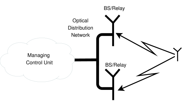
Figure 4: Cloud radio access network communication scenario. Two relays compress and forward the correlated signals they receive from several users.

As we wish to minimize the distortion at the central node subject to the rate constraints, this is a distributed lossy source coding problem. See depiction in Figure 4.

Here, the covariance matrix of the received signals at the relays is given by

$$\mathbf{K}_{\bf xx}=\text{$\mathsf{SNR}$}\mathbf{H}\mathbf{H}^{T}+\mathbf{I}.$$ (53)

We note that we can “absorb” the $\mathsf{SNR}$ into the channel and hence we set $\text{$\mathsf{SNR}$}=1$, so that

$$\mathbf{K}_{\bf xx}=\mathbf{H}\mathbf{H}^{T}+\mathbf{I}.$$ (54)

We further assume that the entries of the channel matrix $\mathbf{H}$ are Gaussian i.i.d., i.e. $\forall_{i,j}\mathbf{H}_{i,j}\sim\mathcal{N}(0,\sigma^{2})$. As mentioned in the introduction, the SVD of this matrix

$$\mathbf{H}=\mathbf{\tilde{U}}\mathbf{\tilde{\Sigma}}\mathbf{\tilde{V}}^{T}$$ (55)

satisfies that $\mathbf{\tilde{U}}$ and $\mathbf{\tilde{V}}$ belong to the CRE. We may therefore express the (random) covariance matrix as

$$\mathbf{K}_{\bf xx}=\mathbf{\tilde{U}}(\mathbf{\tilde{\Sigma}}+\mathbf{I})(\mathbf{\tilde{\Sigma}}+\mathbf{I})^{T}\mathbf{\tilde{U}}^{T},$$ (56)

where $\mathbf{\tilde{U}}$ is drawn from the CRE. It follows that the precoding matrix $\mathbf{P}$ is redundant (as we assumed that $\mathbf{P}$ is also drawn from the CRE). Thus, the analysis above holds also for the considered scenario.

Specifically, assuming the encoders are subject to an equal rate constraint, then for a given distortion level, the relation between the compression rate of IF source coding and the guaranteed outage probability (for meeting the prescribed distortion) is bounded using Theorem 2 above.

We note that just as precoded IF channel coding can be applied to complex channels as described in [3], so can precoded IF source coding be extended to complex Gaussian sources. In describing an outage event in this case we assume that the precoding matrix is drawn from the circular unitary ensemble (CUE). The bounds derived above (replacing $K$ with $2K$ in all derivations) for the relation between the compression rate of IF source coding and the worst-case outage probability hold for the C-RAN scenario over complex Gaussian channels $\mathbf{H}\in\mathbb{C}^{K\times M}$, where the CUE precoding can be viewed as been performed by nature.

V Performance Guarantees for Integer-Forcing Source Coding with Deterministic Precoding

In this section, we consider the performance of IF source coding when used in conjunction with judiciously chosen (deterministic) precoding. Worst-case performance will be measured in a stricter sense than in previous sections; namely, no outage is allowed. We begin by establishing an additive bound applicable for general Gaussian sources, in the form of a constant gap from the Berger-Tang benchmark. Similar to the bound established in [14] for IF channel coding (specifically, Theorem 5 in the latter), the derived gap depends only on the number of sources and the properties of the non-vanishing code which is used as the underlying universal transformation. We note that the derived bound on the gap is even larger than that in the channel coding counterpart and thus its applicability is limited. The reason for the difference in the derived gap is that unlike in the bound of [14], we were unable to use the transference theorem of Banaszczyk [15] and thus resorted to Minkowski’s theorem (as recalled in Appendix C, Theorem 6).

Then, in Section V-B, we consider the special case of independent Gaussian sources having different variances. Here, we use a very different approach for analysis, by which we are able to establish a much tighter bound on the gap to the Berger-Tung benchmark. The derived performance guarantees are tight enough to be useful in practical scenarios, at least for a small number sources.

V-A Additive Bound for General Sources

Similar to the case of channel coding, we can derive a worst-case additive bound for the gap to the Berger-Tung benchmark. Achieving this guaranteed performance requires joint algebraic number-theoretic based space-time precoding at the encoders. The following theorem is due to Or Ordentlich [16].

Theorem 4 (Ordentlich).

For any $K$ sources with covariance matrix $\mathbf{K}_{\bf xx}$ and Berger-Tung benchmark $R_{\rm BT}$, the excess rate with respect to the Berger-Tung benchmark (normalized per the number of time-extensions used) of space-time IF source coding with an NVD precoding matrix with minimum determinant $\delta_{\min}$ is bounded by

$$R_{\rm IF}-R_{\rm BT}\leq 2K^{3}\log(2K^{2})+K^{2}\log\frac{1}{\delta_{\min}}.$$ (57)

Proof.

See Appendix D. ∎

We note that the gap to the Berger-Tung benchmark is large (even larger than the one derived for channel coding IF in [14]) and is thus of limited applicability. Nevertheless, we first note that although the guaranteed gap is large, numerical evidence indicates that true gap is most likely much smaller. Hence, we believe the bound may be significantly tightened. Furthermore, if we relax the no outage restriction, the much tighter bounds of Section IV (using random precoding drawn from the CRE) are directly applicable.

V-B Uncorrelated Sources

For the special case of uncorrelated Gaussian sources, much tighter bounds (in comparison to Theorem 4) on the worst-case quantization rate of IF for a given distortion level may be obtained. First, space-time precoding may be replaced with precoding over space only. This allows to obtain a tighter counterpart to Theorem 4, as derived in Section 2.4.2 of [9].

We next derive yet tighter performance guarantees, also following ideas developed in [9], by numerically evaluating the performance of IF source coding over a “densely” quantized set of source (diagonal) covariance matrices belonging to the compound class, and then bounding the excess rate w.r.t. to the evaluated ones for any possible source vector in the compound class.

In the case of uncorrelated sources, the covariance matrix $\mathbf{K}_{\bf xx}$ is diagonal. Hence, (56) becomes

$$\mathbf{K}_{\bf xx} =\mathbf{\tilde{\Sigma}}\mathbf{\tilde{\Sigma}}^{T}$$

$$\triangleq\mathbf{S},$$ (58)

where

$$\mathbf{S}=\begin{bmatrix}s_{1}^{2}&0&\cdots&0\\ 0&s_{2}^{2}&\cdots&0\\ \vdots&0&\ddots&\vdots\\ 0&0&\cdots&s_{K}^{2}\end{bmatrix}.$$ (59)

We denote ${\bf s}=\mathop{\mathrm{diag}}(\mathbf{S})$. The compound set of sources may be parameterized by

$$\mathcal{S}(R_{\rm BT})=\left\{\mathbf{S}:\sum_{i=1}^{K}\frac{1}{2}\log\left(1+s_{i}^{2}\right)=R_{\rm BT}\right\}.$$ (60)

We note that we may associate with each diagonal element a “rate” corresponding to an individual source

$$R_{i}=\frac{1}{2}\log\left(1+s_{i}^{2}\right).$$ (61)

Thus, the compound class of sources may equivalently be represented by the set of rates

$$\mathcal{R}(R_{\rm BT})=\left\{\left(R_{1},R_{2},\ldots,R_{K}\right)\in\mathbb{R}^{K}:\sum_{i=1}^{K}R_{i}=R_{\rm BT}\right\}.$$ (62)

We define a “quantized” rate-tuple set as follows. The interval $[0,R_{\rm BT}]$ is divided into $N$ sub-intervals, each of length $\Delta=R_{\rm BT}/N$. Thus, the resolution is determined by the parameter $\Delta$. The quantized rate-tuples belong to the grid

$$\mathcal{R}^{\Delta}(R_{\rm BT})=\Bigl{\{}\left(R_{1}^{\Delta},R_{2}^{\Delta},\ldots,R_{K}^{\Delta}\right)\in\Delta\cdot R_{\rm BT}\cdot{\mathbb{Z}^{+}}^{K}:$$

$$\sum_{i=1}^{K}R_{i}^{\Delta}=R_{\rm BT}\Bigr{\}}.$$ (63)

We may similarly define the (non-uniformly) quantized set $\mathcal{S}^{\Delta}(R_{\rm BT})$ of diagonal matrices such that the diagonal entries satisfy $s_{i,\Delta}^{2}=2^{2R_{i}^{\Delta}}-1$, $i=1,\ldots,K$, where $\mathbf{R}^{\Delta}\in\mathcal{R}^{\Delta}(R_{\rm BT})$.

Theorem 5.

For any Gaussian vector of independent sources with covariance matrix $\mathbf{S}$ such that $\mathbf{S}\in\mathcal{S}(R_{\rm BT})$, the rate of IF source coding with a given precoding matrix $\mathbf{P}$ is upper bound by

$$R_{\rm IF}^{\rm opt}(\mathbf{S},\mathbf{P})\leq\max_{\mathbf{S}^{\Delta}\in\mathcal{S}^{\Delta}(R_{\rm BT})}R_{\rm IF}^{\rm opt}\left(\mathbf{S}^{\Delta},\mathbf{P}\right)+K\log\eta$$ (64)

where

$$\eta=\sqrt{\frac{2^{2\left(\frac{R_{\rm BT}}{K}\right)}-1}{2^{2\left(\frac{R_{\rm BT}}{K}-(K-1)\Delta R_{\rm BT}\right)}-1}}.$$ (65)

Proof.

Assume we have a covariance matrix $\mathbf{S}$ in the compound class. Hence, its associated rate-tuple satisfies $(R_{1},R_{2},\ldots,R_{K})\in\mathcal{R}(R_{\rm BT})$. Assume without loss of generality that

$$R_{1}\leq R_{2}\leq\ldots\leq R_{K}.$$ (66)

By (24), the rate of IF source coding associated with a specific integer linear combination vector $\mathbf{a}$ is

$$R_{{\rm IF},k}(\mathbf{S},\mathbf{P};\mathbf{A})=\frac{1}{2}\log\left({\bf a}_{k}^{T}\mathbf{P}\left(\mathbf{I}+\mathbf{S}\right)\mathbf{P}^{T}{\bf a}_{k}\right).$$ (67)

Denote

$${\bf v}={\bf a}_{k}^{T}\mathbf{P}.$$ (68)

We will need the following two lemmas, whose proofs appear in Appendices E and F, respectively.

Lemma 3.

For any diagonal covariance matrix $\mathbf{S}$, associated with a rate-tuple $(R_{1},R_{2},\ldots,R_{K})\in\mathcal{R}(R_{\rm BT})$, there exists a diagonal covariance matrix $\mathbf{S}^{\Delta}$, associated with a rate-tuple $(R^{\Delta}_{1},R^{\Delta}_{2},\ldots,R^{\Delta}_{K})\in\mathcal{R}^{\Delta}(R_{\rm BT})$, such that

$$s_{i}\leq\eta^{2}s_{i,\Delta}^{2}$$ (69)

for $1\leq i\leq K$, where $\eta$ is defined in (65).

Lemma 4.

Consider a Gaussian vector with a diagonal covariance matrix $\mathbf{S}$ and let $\mathbf{A}$ be an invertible integer matrix. Then for any $\beta\geq 1$, we have

$$R_{{\rm IF},k}(\beta^{2}\mathbf{S},\mathbf{P};\mathbf{A})\leq\log\left(\beta\right)+R_{{\rm IF},k}(\mathbf{S},\mathbf{P};\mathbf{A}).$$ (70)

Using Lemma 3, we denote by $\mathbf{S}^{\Delta}$ the covariance matrix associated with $\mathbf{S}$, and whose existence is guaranteed by the lemma. Recalling (21), we have

$$R_{\rm IF}^{\rm opt}({\mathbf{S}^{\Delta}},\mathbf{P})=\frac{K}{2}\log\left(\min_{\begin{subarray}{c}\mathbf{A}\in\mathbb{Z}^{K\times K}\\ \det{\mathbf{A}}\neq 0\end{subarray}}\max_{k=1,...,K}R_{\rm IF}({\mathbf{S}^{\Delta}},\mathbf{P};{\bf a}_{k})\right).$$ (71)

Denoting $\mathbf{A}^{\rm opt}_{\Delta}$ as the optimal integer matrix for the quantized source $\mathbf{S}^{\Delta}$, it follows that

$$R^{\rm opt}_{\rm IF}({\mathbf{S}},\mathbf{P}) =R_{\rm IF}({\mathbf{S}},\mathbf{P};\mathbf{A}^{\rm opt})$$

$$\leq R_{\rm IF}({\mathbf{S}},\mathbf{P};\mathbf{A}^{\rm opt}_{\Delta}),$$ (72)

where the inequality follows since $\mathbf{A}^{\rm opt}_{\Delta}$ is the optimal integer matrix for $\mathbf{S}^{\Delta}$ and not necessarily for $\mathbf{S}$. From (67) and by the definition of $\mathbf{v}$ in (68), we have

$$R_{{\rm IF},k}(\eta^{2}{\mathbf{S}^{\Delta}},\mathbf{P};\mathbf{A}^{\rm opt}_{\Delta}) =\frac{1}{2}\log\left(\sum_{i=1}^{K}{v}_{i}^{2}(1+\eta^{2}{s_{i,\Delta}^{2}})\right)$$

$$\geq\frac{1}{2}\log\left(\sum_{i=1}^{K}{v}_{i}^{2}(1+s_{i}^{2})\right)$$

$$=R_{{\rm IF},k}(\mathbf{S},\mathbf{P};\mathbf{A}^{\rm opt}_{\Delta}).$$ (73)

Using Lemma 4, we further have that

$$R_{{\rm IF},k}(\eta^{2}{\mathbf{S}^{\Delta}},\mathbf{P};\mathbf{A}^{\rm opt}_{\Delta})\leq\frac{1}{2}\log(\eta^{2})+R_{{\rm IF},k}({\mathbf{S}^{\Delta}},\mathbf{P};\mathbf{A}^{\rm opt}_{\Delta}).$$ (74)

Combining (73) and (74), we obtain

$$R_{{\rm IF},k}(\mathbf{S},\mathbf{P};\mathbf{A}^{\rm opt}_{\Delta}) \leq R_{\rm IF}(\eta^{2}{\mathbf{S}^{\Delta}},\mathbf{P};\mathbf{A}^{\rm opt}_{\Delta})$$

$$\leq\log(\eta)+R_{{\rm IF},k}({\mathbf{S}^{\Delta}},\mathbf{P};\mathbf{A}^{\rm opt}_{\Delta}).$$ (75)

We therefore have (75) we have

$$R_{\rm IF}({\mathbf{S}},\mathbf{P};\mathbf{A}^{\rm opt}_{\Delta}) =K\max_{k=1,...,K}R_{{\rm IF},k}({\mathbf{S}},\mathbf{P};\mathbf{A}^{\rm opt}_{\Delta})$$

$$\leq K\max_{k=1,...,K}\bigl{(}\log(\eta)+R_{{\rm IF},k}({\mathbf{S}^{\Delta}},\mathbf{P};\mathbf{A}^{\rm opt}_{\Delta})\bigr{)}$$

$$=K\log(\eta)+R_{\rm IF}(\mathbf{S}^{\Delta},\mathbf{P};\mathbf{A}^{\rm opt}_{\Delta}).$$ (76)

Thus, recalling (72), we conclude that

$$R_{\rm IF}({\mathbf{S}},\mathbf{P};\mathbf{A}^{\rm opt})\leq R_{\rm IF}(\mathbf{S}^{\Delta},\mathbf{P};\mathbf{A}^{\rm opt}_{\Delta})+K\log(\eta)$$ (77)

and therefore, for any $\mathbf{S}\in\mathcal{S}(R_{\rm BT})$, we have

$$R_{\rm IF}^{\rm opt}({\mathbf{S}},\mathbf{P})\leq\max_{\mathbf{S}^{\Delta}\in\mathbb{S}^{\Delta}}R_{\rm IF}^{\rm opt}(\mathbf{S}^{\Delta},\mathbf{P})+K\log(\eta).$$ (78)

This concludes the proof of the theorem.

∎

As an example for the achievable performance, Figure 5 gives the empirical worst-case performance for two and three (real) sources that is achieved when using IF source coding and a fixed precoding matrix over the grid $\mathcal{R}^{\Delta}(R_{\rm BT})$ for $\Delta=0.01$. The precoding matrix was taken from [6]. The explicit precoding matrix used for two sources is $\mathbf{P}=\mathbf{\rm cyclo_{2}}$ where

$$\mathbf{\rm cyclo_{2}}=\begin{bmatrix}-0.5257311121&-0.8506508083\\ -0.8506508083&0.5257311121\end{bmatrix},$$ (79)

and for three sources $\mathbf{P}=\mathbf{\rm cyclo_{3}}$ where

$$\mathbf{\rm cyclo_{3}}=\begin{bmatrix}-0.3279852776&-0.5910090485&-0.7369762291\\ -0.7369762291&-0.3279852776&0.5910090485\\ -0.5910090485&0.7369762291&-0.3279852776\end{bmatrix}.$$ (80)

Rather than plotting the gap from the Berger-Tung benchmark, we plot the efficiency $\frac{R_{IF}}{R_{\rm BT}}$, i.e., the ratio of the (worst-case) rate of IF source coding and $R_{\rm BT}$. We also plot the upper bound on $R_{\rm IF}(\mathbf{S},\mathbf{P})$ given by Theorem 5. As is apparent from Figure 5, the guaranteed efficiency approaches $1$ quite rapidly as the quantization rate grows.

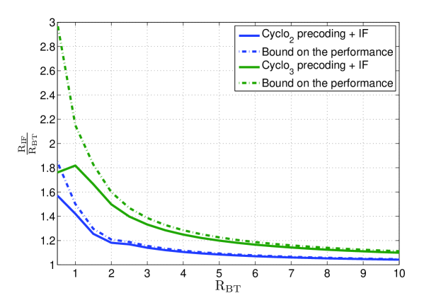
Figure 5: Empirical and guaranteed (upper bound) worst-case efficiency of IF source coding for two and three uncorrelated Gaussian sources, when using the precoding matrices $\mathbf{\rm cyclo_{2}}$ and $\mathbf{\rm cyclo_{3}}$ given in (79)-(80), respectively, and taking $\Delta=0.01$ for the calculation of Theorem 5.

VI Summary

It has been observed in previous works that integer-forcing source coding is a very effective method for compression of distributed Gaussian sources, for “most” but not all source covariance matrices. In the present work we have quantified the measure of bad covariance matrices by characterizing the probability that integer-forcing source coding fails as a function of the allocated rate, where the probability is with respect to a random orthonormal transformation that is applied to the sources prior to quantization. This characterization is directly applicable to the case where the signals to be compressed correspond to the antenna inputs of relays in an i.i.d. Rayleigh fading environment, as in such a scenario the transformation can be viewed as being done by nature.

Integer-forcing source coding is also useful in a non-distributed scenario, where the integer-forcing scheme offers a universal, yet practical, compression method using equal-rate quantizers. Specifically, quantization is performed after passing the sources through an algebraic number theoretic based space-time transformation, followed by a modulo operation. We have obtained constant-gap universal bounds on the maximal possible rate loss when integer-forcing source is used in such a scenario. Further, we have shown that when it is known that the sources are uncorrelated but may be of different variances, applying a space-only transformation is sufficient to attain universal performance guarantees and moreover that the resulting bound on the maximal possible rate loss is much smaller than for the general case. An interesting avenue for further research is to try to generalize the numerical bounding technique applied in Section  V-B to obtain tighter bounds for the performance of precoded integer-forcing source coding of general Gaussian sources.

Appendix A Proof of Theorem 1

Following the footsteps of Lemma 2 in [3] and adopting the same geometric interpretation described there, we may interpret ${\rm Pr}\left(\|\mathbf{D}^{-1/2}\mathbf{U}^{T}{\bf a}\|<\sqrt{{\beta}}\right)$ as the ratio of the surface area of an ellipsoid that is inside a ball with radius $\sqrt{{\beta}}$ and the surface area of the entire ellipsoid. The axes of this ellipsoid are defined by $x_{i}=\frac{\|{\bf a}\|}{\sqrt{d_{i}}}$.

Denote the vector ${\bf o}_{\|{\bf a}\|}$ as a vector drawn from the CRE with norm $\|{\bf a}\|$. Using Lemma 1 in [3] and since we assume that $\mathbf{U}^{T}$ is drawn from the CRE, we have that the right hand side of (44) is equal to

$$\sum_{{\bf a}\in{\mathbb{A}({\beta},1/d_{\max},K)}}{\rm Pr}\left(\|\mathbf{D}^{-1/2}{\bf o}_{\|{\bf a}\|}<\sqrt{{\beta}}\right)$$

$$=\sum_{{\bf a}\in{\mathbb{A}({\beta},1/d_{\max},K)}}\frac{\rm CAP_{\rm ell}(x_{1},\cdots,x_{K})}{L(x_{1},\cdots,x_{K})}$$ (81)

where

$${\rm CAP_{\rm ell}(x_{1},\cdots,x_{K})}<K\frac{\pi^{K/2}}{\Gamma(1+K/2)}\sqrt{{\beta}}^{K-1}\triangleq\overline{\rm CAP_{\rm ell}},$$ (82)

and

$${L(x_{1},\cdots,x_{K})} >\frac{\pi^{K/2}}{\Gamma(1+K/2)}\frac{\|{\bf a}\|^{K}}{\prod_{i=1}^{K}\sqrt{d_{i}}}\sum_{i=1}^{K}\frac{\sqrt{d_{i}}}{\|{\bf a}\|}$$ (83)

$$>\frac{\pi^{K/2}}{\Gamma(1+K/2)}\frac{\|{\bf a}\|^{K-1}{\sqrt{d_{\max}}}}{2^{R_{\rm BT}}}\triangleq\underline{L}.$$ (84)

Substituting (82) and (84) in (81), we obtain

$$\sum_{{\bf a}\in{\mathbb{A}({\beta},1/d_{\max},K)}}\frac{\rm CAP_{\rm ell}(x_{1},\cdots,x_{K})}{L(x_{1},\cdots,x_{K})}$$

$$<\sum_{{\bf a}\in{\mathbb{A}({\beta},1/d_{\max},K)}}\frac{\overline{\rm CAP_{\rm ell}}}{\underline{L}}$$

$$=\sum_{{\bf a}\in{\mathbb{A}({\beta},1/d_{\max},K)}}\frac{K{\sqrt{{\beta}}}^{K-1}}{\frac{\|{\bf a}\|^{K-1}}{2^{R_{\rm BT}}}{\sqrt{d_{\max}}}}.$$ (85)

Recalling (see (38)) that ${\beta}=\alpha(K)2^{-\frac{2}{K}(R_{\rm BT}+\Delta R)}$, we obtain

$${\rm Pr}\left(R_{\rm IF-SUC}^{\rm opt}(\mathbf{D},\mathbf{U})>R_{\rm BT}+\Delta R\right)$$

$$<\sum_{{\bf a}\in\mathbb{A}({\beta},1/d_{\max},K)}\frac{K\alpha(K)^{\frac{K-1}{2}}2^{-\frac{K-1}{K}(R_{\rm BT}+\Delta R)}}{\frac{\|{\bf a}\|^{K-1}}{2^{R_{\rm BT}}}{\sqrt{d_{\max}}}}.$$ (86)

Appendix B Proof of Theorem 2

To establish Theorem 2, we follow the footsteps of the proof of Theorem 2 in [3] to obtain

$$\sum_{{\bf a}\in{\mathbb{A}({\beta},1/d_{\max},K)}}{\rm Pr}\left(\|\mathbf{D}^{-1/2}\mathbf{U}^{T}{\bf a}\|<\sqrt{{\beta}}\right)$$

$$\leq\sum_{{\bf a}\in{\mathbb{A}({\beta},1/d_{\max},K)}}\frac{K{\sqrt{{\beta}}}^{K-1}}{\frac{\|{\bf a}\|^{K-1}}{2^{R_{\rm BT}}}{\sqrt{d_{\max}}}}$$ (87)

where $\mathbb{A}({\beta},1/d_{\max},K)$ and ${\beta}$ are defined in (29) and (38), respectively. Noting that

$$\mathbb{A}({\beta},1/d_{\max},K)\subseteq\left\{\mathbf{a}:\|\mathbf{a}\|\leq\left\lfloor\sqrt{{{\beta}}{d_{\max}}}\right\rfloor+1\right\},$$

the summation in (87) can be bounded as

$$\leq\sum^{\lfloor\sqrt{{\beta}d_{\max}}\rfloor}_{k=0}\sum_{k<\|{\bf a}\|\leq k+1}\frac{K{\sqrt{{\beta}}}^{K-1}}{\frac{k^{K-1}}{2^{R_{\rm BT}}}{\sqrt{d_{\max}}}}$$ (88)

We apply Lemma 1 in [17] (a bound for the number of integer vectors contained in a ball of a given radius). Using this bound while noting that when $\|{\bf a}\|=1$ there are exactly $K$ integer vectors, the right hand side of (88) may be further bounded as

$$\leq\frac{K{\sqrt{{\beta}}}^{K-1}2^{R_{\rm BT}}}{{\sqrt{d_{\max}}}}{\rm Vol}(\mathcal{B}_{K}(1))\times\left[K+\sum^{\lfloor\sqrt{{\beta}d_{\max}}\rfloor}_{k=1}\right.$$

$$\left.~{}~{}~{}~{}~{}~{}~{}\frac{\left(k+1+\frac{\sqrt{K}}{2}\right)^{K}-\left(\max\left(k-\frac{\sqrt{K}}{2},0\right)\right)^{K}}{k^{K-1}}\right]$$ (89)

where we note that (89) trivially holds when $\left\lfloor\sqrt{{{\beta}}{d_{\max}}}\right\rfloor=0$ since $\mathbb{A}({\beta},1/d_{\max},K)$ is the empty set in this case and hence the left hand side of (81) evaluates to zero.

The right hand side of (89) can further be rewritten as

$$\frac{K{\sqrt{{\beta}}}^{K-1}2^{R_{\rm BT}}}{{\sqrt{d_{\max}}}}{\rm Vol}(\mathcal{B}_{K}(1))\times\left[\underbrace{K}_{\rm I}+\underbrace{\sum^{\left\lfloor\frac{\sqrt{K}}{2}\right\rfloor}_{k=1}\frac{\left(k+1+\frac{\sqrt{K}}{2}\right)^{K}}{k^{K-1}}}_{\rm II}+\right.$$

$$\left.\underbrace{\sum^{\left\lfloor\sqrt{{{\beta}d_{\max}}}\right\rfloor}_{k=\left\lfloor\frac{\sqrt{K}}{2}\right\rfloor+1}\frac{\left[\left(k+1+\frac{\sqrt{K}}{2}\right)^{K}-\left(k-\frac{\sqrt{K}}{2}\right)^{K}\right]}{k^{K-1}}}_{\rm III}\right].$$ (90)

We search for $c_{1}$ and $c_{2}$ (independent of $k$) such that

$$\left(k+1+\frac{\sqrt{K}}{2}\right)^{K}\leq c_{1}k^{K-1}$$ (91)

for $1\leq k\leq\left\lfloor\frac{\sqrt{K}}{2}\right\rfloor$, and

$$\left[\left(k+1+\frac{\sqrt{K}}{2}\right)^{K}-\left(k-\frac{\sqrt{K}}{2}\right)^{K}\right]\leq c_{2}k^{K-1}$$ (92)

for $k\geq 1$, since it will then follow that

$$II+III \leq\sum^{\left\lfloor\sqrt{{{\beta}d_{\max}}}\right\rfloor}_{k=1}\max(c_{1},c_{2})$$

$$={\left\lfloor\sqrt{{{\beta}d_{\max}}}\right\rfloor}\max(c_{1},c_{2}).$$ (93)

We note that since (again assuming $\left\lfloor\sqrt{{{\beta}}{d_{\max}}}\right\rfloor\geq 1$)

$$K\leq\sum^{\left\lfloor\sqrt{{{\beta}}{d_{\max}}}\right\rfloor}_{k=1}K,$$ (94)

it will thus follow that

$$I+II+III \leq\sum^{\left\lfloor\sqrt{{{\beta}}{d_{\max}}}\right\rfloor}_{k=1}\left[K+\max(c_{1},c_{2})\right]$$

$$={\left\lfloor\sqrt{{{\beta}}{d_{\max}}}\right\rfloor}\left[K+\max(c_{1},c_{2})\right].$$ (95)

An explicit derivation for $c_{1}$ and $c_{2}$ appears in Appendix B of [3] (where $2N_{t}$ should be replaced with $K$), from which we obtain

$$c_{1} =\left(1+\sqrt{K}\right)^{K}$$

$$c_{2} =\left[\left(2+\frac{\sqrt{K}}{2}\right)^{K}-\left(1-\frac{\sqrt{K}}{2}\right)^{K}\right].$$ (96)

In is also shown in Appendix B of [3] that for $K\geq 4$, $c_{2}\leq c_{1}$ holds. For $1\leq K<4$ we observe that $c_{1}\leq c_{2}$. This is so since $K<4$ implies that $1-\frac{\sqrt{K}}{2}>0$, and hence indeed for $K<4$ we have

$$c_{2} =\left[\left(2+\frac{\sqrt{K}}{2}\right)^{K}-\left(1-\frac{\sqrt{K}}{2}\right)^{K}\right]$$

$$=\left(1+\sqrt{K}+1-\frac{\sqrt{K}}{2}\right)^{K}-\left(1-\frac{\sqrt{K}}{2}\right)^{K}$$

$$\geq(1+\sqrt{K})^{K}$$

$$=c_{1}.$$ (97)

Recalling now (95) and denoting

$$c_{\max}=\begin{cases}c_{2}~{}~{}~{}1\leq K<4\\ c_{1}~{}~{}~{}K\geq 4\end{cases},$$ (98)

it follows that

$$I+II+III \leq{\left\lfloor\sqrt{{{\beta}d_{\max}}}\right\rfloor}(K+c_{\max}).$$ (99)

Using (99) and substituting the volume of a unit ball ${\rm Vol}(\mathcal{B}_{K}(1))=\frac{\pi^{K/2}}{\Gamma(K/2+1)}$, it follows that right hand side of (89) is upper bounded by

$$\frac{K{\sqrt{{\beta}}}^{K-1}2^{R_{\rm BT}}}{{\sqrt{d_{\max}}}}\frac{\pi^{K/2}}{\Gamma(K/2+1)}\sqrt{{\beta}d_{\max}}(K+c_{\max})$$ (100)

$$=K{\sqrt{{\beta}}}^{K}2^{R_{\rm BT}}(K+c_{\max})\frac{\pi^{K/2}}{\Gamma(K/2+1)}.$$ (101)

Finally, we substitute ${\beta}$, as defined in (38), into (101) to obtain

$$\sum_{{\bf a}\in{\mathbb{A}({\beta},1/d_{\max},K)}}{\rm Pr}\left(\|\mathbf{D}^{-1/2}\mathbf{U}^{T}{\bf a}\|<\sqrt{{\beta}}\right)$$

$$\leq K\left(\alpha(K)2^{-\frac{2}{K}(R_{\rm BT}+\Delta R)}\right)^{K/2}2^{R_{\rm BT}}(K+c_{\max})$$

$$\leq K\left(\alpha(K)\right)^{K/2}2^{-(R_{\rm BT}+\Delta R)}2^{R_{\rm BT}}(K+c_{\max})$$

$$\leq K\left(\alpha(K)\right)^{K/2}(K+c_{\max})2^{-\Delta R}$$

$$=c(K)2^{-\Delta R},$$ (102)

where $c(K)$ is as defined in (48).

Appendix C Proof of Lemma 2 and Theorem 3

We first recall a theorem of Minkowski [18, Theorem 1.5] that upper bounds the product of the successive minima.

Theorem 6 (Minkowski).

For any lattice $\Lambda(\mathbf{F}^{T})$ that is spanned by a full rank $K\times K$ matrix $\mathbf{F}^{T}$

$$\prod_{m=1}^{K}\lambda_{m}^{2}(\mathbf{F}^{T})\leq K^{K}(\det{\mathbf{F}^{T}})^{2}.$$ (103)

To prove Theorem 3, we further need the following two lemmas.

Lemma 5.

For a Gaussian source vector with covariance matrix $\mathbf{K_{xx}}\in\mathcal{K}(R_{\rm BT})$, and for any full-rank integer matrix $\mathbf{A}$, the sum-rate of IF-SUC satisfies

$$\sum_{m=1}^{K}R_{{\rm IF-SUC},m}(\mathbf{K}_{\bf xx};\mathbf{A})=R_{\rm BT}+\log|\det(A)|,$$ (104)

where $R_{{\rm IF-SUC},m}(\mathbf{K}_{\bf xx};\mathbf{A})$ is defined in (19).

Proof.

$$\sum_{m=1}^{K}R_{{\rm IF-SUC},m}(\mathbf{K}_{\bf xx};\mathbf{A}) =\frac{1}{2}\sum_{m=1}^{K}\log(\ell_{m,m}^{2})$$

$$=\frac{1}{2}\log\left(\prod_{m=1}^{K}\ell_{m,m}^{2}\right)$$

$$=\frac{1}{2}\log\det(\mathbf{L}\mathbf{L}^{T})$$

$$=\frac{1}{2}\log\det\left(\mathbf{A}\left(\mathbf{I}+\frac{1}{d}\mathbf{K}_{\bf xx}\right)\mathbf{A}^{T}\right)$$

$$=R_{\rm BT}+\log|\det(A)|$$ (105)

∎

Theorem 3 in [19] shows that for successive IF (used for channel coding) there is no loss (in terms of achievable rate) in restricting $\mathbf{A}$ to the class of unimodular matrices. We note that same claim holds also in our framework (that of successive integer-source coding) by replacing $\mathbf{G}$, the matrix spanning the lattice which was defined in Theorem 3 as

$$\left(\mathbf{I}+\text{$\mathsf{SNR}$}\mathbf{H}\mathbf{H}^{T}\right)^{-1}=\mathbf{G}\mathbf{G}^{T}$$ (106)

with $\mathbf{F}$, as defined in (12), and noting that the optimal $\mathbf{A}$ can be expressed (in both cases) as

$$\mathbf{A}^{\rm opt}_{\rm SIC/SUC}=\min_{\begin{subarray}{c}\mathbf{A}\in\mathbb{Z}^{K\times K}\\ \det{\mathbf{A}}\neq 0\end{subarray}}\max_{k=1,...,K}\ell_{k,k}^{2},$$ (107)

where $\ell_{k,k}$ are the diagonal elements of the corresponding $\mathbf{L}$ matrix (derived from the Cholesky decomposition) in each case.

Having established that the optimal $\mathbf{A}$ is unimodular, it now follows that $\sum_{m=1}^{K}R_{{\rm IF-SUC},m}(\mathbf{K}_{\bf xx};\mathbf{A}^{\rm opt}_{\rm SUC})=R_{\rm BT}$.

We are now ready to prove the following lemma that is analogous to Theorem 3 in [20]. First, denote by

$$R_{{\rm IF},k}(\mathbf{K}_{\bf xx};\mathbf{A})\triangleq\frac{1}{2}\log\left({\bf a}_{k}^{T}\left(\mathbf{I}+\mathbf{K}_{\bf xx}\right){\bf a}_{k}\right)$$ (108)

the effective rate that of the $k$’th equation as appears in the definition of the achievable rate of integer-forcing source coding in (11). Then, we have the following.

Lemma 6.

For a Gaussian source vector with covariance matrix $\mathbf{K_{xx}}\in\mathcal{K}(R_{\rm BT})$, and for the optimal integer matrix $\mathbf{A}^{\rm opt}$, the sum-rate of IF is upper bounded as

$$\sum_{m=1}^{K}R_{{\rm IF},m}(\mathbf{K}_{\bf xx};\mathbf{A}^{\rm opt}) \leq R_{\rm BT}+\frac{K}{2}\log(K).$$ (109)

Proof.

$$\sum_{m=1}^{K}R_{{\rm IF},m}(\mathbf{K}_{\bf xx};\mathbf{A}^{\rm opt}) =\sum_{m=1}^{K}\frac{1}{2}\log\left(\lambda_{m}^{2}(\mathbf{F}^{T})\right)$$

$$=\frac{1}{2}\log\left(\prod_{m=1}^{K}\lambda_{m}^{2}(\mathbf{F}^{T})\right)$$

$$\leq\frac{1}{2}\log\left(K^{K}|\det(F)|^{2}\right)$$

$$=R_{\rm BT}+\frac{K}{2}\log\left(K\right).$$ (110)

where the inequality is due to Theorem 6 (Minkowski’s Theorem). ∎

Now, for the case of two sources we have by Lemma 5

$$R_{{\rm IF-SUC},1}(\mathbf{K}_{\bf xx};\mathbf{A}^{\rm opt}_{\rm SUC})+R_{{\rm IF-SUC},2}(\mathbf{K}_{\bf xx};\mathbf{A}^{\rm opt}_{\rm SUC})=R_{\rm BT},$$ (111)

or equivalently

$$R_{{\rm IF-SUC},2}(\mathbf{K}_{\bf xx};\mathbf{A}^{\rm opt}_{\rm SUC})=R_{\rm BT}-R_{{\rm IF-SUC},1}(\mathbf{K}_{\bf xx};\mathbf{A}^{\rm opt}_{\rm SUC}).$$ (112)

We further have by lemma 6 that

$$R_{{\rm IF},1}(\mathbf{K}_{\bf xx};\mathbf{A}^{\rm opt})+R_{{\rm IF},2}(\mathbf{K}_{\bf xx};\mathbf{A}^{\rm opt})\leq R_{\rm BT}+1.$$ (113)

We note that the (optimal) integer matrix $\mathbf{A}^{\rm opt}$ used for IF in (113) is in general different than the (optimal) matrix $\mathbf{A}^{\rm opt}_{\rm SUC}$ used for IF-SUC in (111)-(112). Nonetheless, when applying IF-SUC, one decodes first the equation with the lowest rate. Since for this equation SUC has no effect, it follows that the first row of $\mathbf{A}$ is the same in both cases and hence

$$R_{{\rm IF-SUC},1}(\mathbf{K}_{\bf xx};\mathbf{A}^{\rm opt}_{\rm SUC})=R_{{\rm IF},1}(\mathbf{K}_{\bf xx};\mathbf{A}^{\rm opt}).$$ (114)

Since source $1$ is decoded first, it follows that $R_{{\rm IF},1}>R_{{\rm IF},2}$ and hence

$$R_{{\rm IF},1}(\mathbf{K}_{\bf xx};\mathbf{A}^{\rm opt})\leq\frac{R_{\rm BT}+1}{2}.$$ (115)

Therefore,

$$R_{\rm IF-SUC}^{\rm opt}(\mathbf{K}_{\bf xx}) =2\max\left(R_{{\rm IF-SUC},1}(\mathbf{K}_{\bf xx};\mathbf{A}^{\rm opt}_{\rm SUC}),R_{{\rm IF-SUC},2}(\mathbf{K}_{\bf xx};\mathbf{A}^{\rm opt}_{\rm SUC})\right)$$

$$\leq 2\max\left(\frac{R_{\rm BT}+1}{2},R_{\rm BT}-R_{{\rm IF},1}(\mathbf{K}_{\bf xx};\mathbf{A}^{\rm opt})\right)$$

$$=\max\left(R_{\rm BT}+1,2R_{\rm BT}-2R_{{\rm IF},1}(\mathbf{K}_{\bf xx};\mathbf{A}^{\rm opt})\right).$$ (116)

Henceforth, we analyze the outage for $R_{\rm BT}>1$ and target rates that are no smaller than $R_{\rm BT}+1$, so that the inequality $2R_{\rm BT}-2R_{{\rm IF},1}(\mathbf{K}_{\bf xx})>R_{\rm BT}+1$ is satisfied. Thus, we consider excess rate values satisfying $\Delta R>1$. Our goal is to bound

$${\rm Pr}\left(R_{\rm IF-SUC}^{\rm opt}(\mathbf{K}_{\bf xx})\geq R_{\rm BT}+\Delta R\right)$$

$$={\rm Pr}\left(2R_{\rm BT}-2R_{{\rm IF},1}(\mathbf{K}_{\bf xx};\mathbf{A}^{\rm opt}_{\rm SUC})\geq R_{\rm BT}+\Delta R\right)$$

$$={\rm Pr}\left(R_{{\rm IF},1}(\mathbf{K}_{\bf xx};\mathbf{A}^{\rm opt})\leq\frac{R_{\rm BT}-\Delta R}{2}\right)$$

$$={\rm Pr}\left(\frac{1}{2}\log(\lambda_{1}^{2}(\mathbf{F}^{T}))\leq\frac{R_{\rm BT}-\Delta R}{2}\right)$$

$$={\rm Pr}\left(\lambda_{1}^{2}(\mathbf{F}^{T})\leq 2^{R_{\rm BT}-\Delta R}\right)$$ (117)

Let ${\beta}=2^{R_{\rm BT}-\Delta R}$. We wish to bound (117), or equivalently

$${\rm Pr}\left(\lambda_{1}^{2}(\mathbf{F}^{T})\leq{\beta}\right)={\rm Pr}\left(\lambda_{1}(\mathbf{F}^{T})\leq\sqrt{{\beta}}\right)$$ (118)

for a given matrix $\mathbf{D}$ corresponding to $\mathbf{K}_{\bf xx}$ (via the relation (22)). Note that the event $\lambda_{1}(\Lambda)<\sqrt{{\beta}}$ is equivalent to the event

$$\bigcup_{\bf{a}\in{\mathbb{Z}^{K}\setminus\{{\bf 0}\}}}||\mathbf{D}^{1/2}\mathbf{U}^{T}\bf{a}||<\sqrt{{\beta}}.$$ (119)

Applying the union bound yields

$${\rm Pr}\left(\lambda_{1}(\Lambda)<\sqrt{{\beta}}\right)\leq\sum_{{\bf a}\in{\mathbb{Z}^{K}\setminus\{{\bf 0}\}}}{\rm Pr}\left(||\mathbf{D}^{1/2}\mathbf{U}^{T}{\bf a}||<\sqrt{{\beta}}\right).$$ (120)

Using the same derivation as in Lemma 2 in [3], we get

$${\rm Pr}\left(R_{\rm IF-SUC}^{\rm opt}(\mathbf{D},\mathbf{U})\geq R_{\rm BT}+\Delta R\right)$$

$$\leq\sum_{{\bf a}\in\mathbb{A}({\beta},d_{\min},K)}\frac{K\sqrt{{\beta}}^{K-1}}{\|{\bf a}\|^{K-1}2^{R_{\rm BT}}\frac{1}{\sqrt{d_{\min}}}}.$$ (121)

Since we are analyzing the case of two sources, we have

$${\rm Pr}\left(R^{\rm opt}_{\rm IF-SUC}(\mathbf{D},\mathbf{U})\geq R_{\rm BT}+\Delta R\right)$$

$$\leq\sum_{{\bf a}\in\mathbb{A}({\beta},d_{\min},K)}\frac{2\sqrt{{\beta}}}{\|{\bf a}\|2^{R_{\rm BT}}\frac{1}{\sqrt{d_{\min}}}}.$$ (122)

This establishes Lemma 2.

Applying a similar argument as appears in Appendix B (as part of the proof of Theorem 2), and noting that $K<4$ implies that $c_{\max}=c_{2}$, we get

$${\rm Pr}\left(R^{\rm opt}_{\rm IF-SUC}(\mathbf{D},\mathbf{U})\geq R_{\rm BT}+\Delta R)\right)$$

$$\leq\frac{2{\beta}}{2^{R_{\rm BT}}}\left(2+3+3\sqrt{2}\right)\pi.$$ (123)

Finally, substituting ${\beta}$ as defined in (38), we obtain

$${\rm Pr}\left(R^{\rm opt}_{\rm IF-SUC}(\mathbf{D},\mathbf{U})\geq R_{\rm BT}+\Delta R\right)$$

$$\leq\frac{2\pi\cdot 2^{R_{\rm BT}-\Delta R}}{2^{R_{\rm BT}}}\left(2+3+3\sqrt{2}\right)$$

$$=2\pi\left(5+3\sqrt{2}\right)2^{-\Delta R}.$$ (124)

Appendix D Additive (Worst-Case) Bound for NVD Space-Time Precoded Sources

Combining space-time precoding and integer forcing in the context of channel coding was suggested in [21], as we next briefly recall. We then present the necessary modifications for the case of source coding.

We derive below an additive bound using a unitary precoding matrix satisfying a non-vanishing determinant (NVD) property. As the theory of NVD space-time codes has been developed over the complex field, it will prove convenient for us to employ complex precoding matrices. To this end, we may assume that we stack samples from two time slots where the samples stacked at the first time slot represent the real part of a complex number and the samples stacked at the second time slot represent the imaginary part of a complex number. Hence, we have

$$\mathbf{K}_{\hat{x}\hat{x}} =\mathbf{I}_{2\times 2}\otimes\mathbf{K}_{xx},$$ (125)

where $\otimes$ is the Kronecker product. We note that the Berger-Tung benchmark of this stacked source vector is

$$R_{\rm BT}(\mathbf{K}_{\hat{x}\hat{x}})=2R_{\rm BT}(\mathbf{K}_{{x}{x}}).$$ (126)

Next, in order to allow space-time precoding, we stack $T$ times the $K$ “complex” outputs of the $K$ sources and let $\bar{\boldsymbol{x}}_{c}\in\mathbb{R}^{2KT\times 1}$ denote the effective source vector. Its correlation matrix, which we refer to as the effective covariance matrix, takes the form

$$\mathcal{K} =\mathbf{I}_{T\times T}\otimes\mathbf{K}_{\hat{x}\hat{x}}.$$ (127)

We assume a precoding matrix, that in principle can be either deterministic or random, is applied to the effective source vector. We analyze performance for the case where the precoding matrix $\mathbf{P}_{st,c}$ is deterministic, specifically a precoding matrix induced by a perfect space-time block code, operating on the stacked source $\bar{\boldsymbol{x}}_{c}$ having covariance matrix as given in (127). An explanation on how to extract the precoding matrix from a space-time code can be found in Section IV in [14].

We denote the corresponding precoding matrix over the reals as $\mathbf{P}_{st}\in\mathbb{R}^{2KT\times 2KT}$. We denote

$$\mathbf{I}+\mathbf{P}_{st}\mathcal{K}\mathbf{P}_{st}^{H}=\mathcal{F}\mathcal{F}^{T}.$$ (128)

As we assume that the precoding matrix is unitary, the Berger-Tung benchmark (normalized by the total number of time extensions used) remains unchanged, i.e.,

$$\frac{1}{2T}\frac{1}{2}\log\det\left(\mathbf{I}+\mathbf{P}_{st}\mathcal{K}\mathbf{P}_{st}^{H}\right) =\frac{1}{2T}\frac{1}{2}\log\left(\det\mathcal{F}^{T}\right)^{2}$$

$$=R_{\rm BT}.$$ (129)

As noted above, we assume that the generating matrix of a perfect code [22, 23] is employed as a precoding matrix.

A space-time code is called perfect if:

• It is full rate;

• It satisfies the non-vanishing determinant (NVD) condition;

• The code’s generating matrix is unitary.

Let $\delta_{\min}$ denote the minimal non-vanishing determinant of this code. Such codes further use the minimal number of time extensions possible, i.e., $T=K$. Thus, we have a total of $K^{2}$ stacked complex samples. Subsisting $2K^{2}$ as the dimension (number of real samples jointly processed) in (16), the rate of IF source coding for the time-stacked samples is given by

$$R_{\rm IF}^{\rm opt}(\mathcal{K},\mathbf{P}_{st})=(2K^{2})\frac{1}{2}\log\left(\lambda_{2K^{2}}^{2}(\mathcal{F}^{T})\right).$$ (130)

To bound $\lambda_{2K^{2}}^{2}(\mathcal{F}^{T})$, we note that for every $2K^{2}$-dimensional lattice, we have

$$\lambda_{1}^{2(2K^{2}-1)}(\mathcal{F}^{T})\lambda_{2K^{2}}^{2}(\mathcal{F}^{T})\leq\prod_{m=1}^{2K^{2}}\lambda_{m}^{2}(\mathcal{F}^{T}).$$ (131)

Using Minkowski’s theorem (Theorem 6 in Appendix C), it follows that

$$\lambda_{2K^{2}}^{2}(\mathcal{F}^{T})\leq(2K^{2})^{2K^{2}}(\det{\mathcal{F}^{T}})^{2}\frac{1}{\lambda_{1}^{2(2K^{2}-1)}(\mathcal{F}^{T})}.$$ (132)

Hence, the rate of IF source coding (normalized by the number of time extensions) can be bounded as:

$$\frac{1}{2K}R_{\rm IF}^{\rm opt}(\mathcal{K},\mathbf{P}_{st})$$

$$=\frac{1}{2K}(2K^{2})\frac{1}{2}\log\left(\lambda_{2K^{2}}^{2}(\mathcal{F}^{T})\right)$$

$$\leq\frac{K}{2}\log\left((2K^{2})^{2K^{2}}(\det{\mathcal{F}^{T}})^{2}\frac{1}{\lambda_{1}^{2(2K^{2}-1)}(\mathcal{F}^{T})}\right)$$

$$=K^{3}\log(2K^{2})+\frac{K}{2}\log(\det({\mathcal{F}^{T}})^{2})-\frac{K(2K^{2}-1)}{2}\log(\lambda_{1}^{2}(\mathcal{F}^{T}))$$

$$=K^{3}\log(2K^{2})+2K^{2}R_{\rm BT}-\frac{K(2K^{2}-1)}{2}\log(\lambda_{1}^{2}(\mathcal{F}^{T})).$$ (133)

We next use the results derived in [14] for channel coding (using NVD precoding). We note that since the covariance matrix is positive semi-definite, it may be written as

$$\mathbf{K}_{{x}{x}}=\mathbf{H}\mathbf{H}^{T}.$$ (134)

The covariance matrix of the stacked source vector may be written as

$$\mathbf{K}_{\hat{x}\hat{x}}=\mathbf{\hat{H}}\mathbf{\hat{H}}^{T},$$ (135)

where we may take $\mathbf{\hat{H}}=\mathbf{I}_{2\times 2}\otimes\mathbf{H}$.

There are many such choices of $\mathbf{H}$ and any such choice corresponds to a channel matrix $\mathbf{\hat{H}}$ that can be viewed as the real representation of a complex channel matrix (which in the present case is real, i.e., has no imaginary part) in the context of [14]. The effective covariance matrix can similarly be rewritten as

$$\mathcal{K}=\mathcal{H}\mathcal{H}^{T},$$ (136)

where $\mathcal{H}=\mathbf{I}_{T\times T}\otimes\mathbf{\hat{H}}$.

Using the channel coding terminology of [14], we further define the minimum distance at the receiver $d_{\rm min}(\mathbf{H},L)$ as

$$d_{\rm min}(\mathbf{H},L)\triangleq\min_{\bf{a}\in{\rm QAM}^{K}(L)\backslash 0}\|\mathbf{H}{\bf a}\|,$$ (137)

where

$${\rm QAM}(L)\triangleq \{-L,-L+1,\ldots,L-1,L\}$$

$$+i\{-L,-L+1,\ldots,L-1,L\}.$$ (138)

Setting $\text{$\mathsf{SNR}$}=1$ and for $\mathbf{\hat{H}}\in\mathbb{R}^{2K\times 2K}$ (which is the real representation of $\mathbf{H}_{c}\in\mathbb{C}^{K\times K}$), Lemma 2 in [14] states that

$$\frac{1}{4K^{4}}\min_{{\bf a}\in\mathbb{Z}^{2K}\setminus 0}{\bf a}^{T}\left(\mathbf{I}+\mathbf{P}_{st}^{H}\mathcal{H}^{H}\mathcal{H}\mathbf{P}_{st}\right){\bf a}$$

$$\geq\frac{1}{4K^{4}}\min_{L=1,2,\cdots}\left(L^{2}+\text{$\mathsf{SNR}$}d_{\min}(\mathcal{H}\mathbf{P}_{st},L)\right).$$ (139)

Using Corollary 1 in [14], we get

$$\frac{1}{4K^{4}}\min_{{\bf a}\in\mathbb{Z}^{2K}\setminus 0}{\bf a}^{T}\left(\mathbf{I}+\mathbf{P}_{st}^{H}\mathcal{H}^{H}\mathcal{H}\mathbf{P}_{st}\right){\bf a}$$

$$\geq\frac{1}{4K^{4}}\min_{L=1,2,\cdots}\left(L^{2}+\left[\delta_{\min}^{\frac{1}{K}}2^{\frac{C_{\rm WI}}{K}}-2K^{2}L^{2}\right]^{+}\right)$$

$$\geq\frac{1}{4K^{4}}\min_{L=1,2,\cdots}\left(L^{2}+\left[\frac{\delta_{\min}^{\frac{1}{K}}2^{\frac{C_{\rm WI}}{K}}}{2K^{2}}-L^{2}\right]^{+}\right)$$

$$\geq\frac{1}{8K^{6}}\delta_{\min}^{\frac{1}{K}}2^{\frac{C_{\rm WI}}{K}},$$ (140)

where $C_{\rm WI}=\frac{1}{2}\log\det\left(\mathbf{I}+\mathbf{H}^{H}\mathbf{H}\right)$ is the mutual information of $\mathbf{H}$. Since $C_{\rm WI}$ is the rate of a $2K\times 2K$ real matrix (resulting from a $K\times K$ complex matrix), it equals $R_{\rm BT}(\mathbf{K}_{\hat{x}\hat{x}})$ defined in (126). Hence, we obtain

$$\min_{{\bf a}\in\mathbb{Z}^{2K}\setminus 0}{\bf a}^{T}\left(\mathbf{I}+\mathbf{P}_{st}^{H}\mathcal{H}^{H}\mathcal{H}\mathbf{P}_{st}^{H}\right){\bf a}\geq\frac{1}{2K^{2}}\delta_{\min}^{\frac{1}{K}}2^{\frac{2R_{\rm BT}}{K}}$$ (141)

which in turn yields

$$\lambda_{1}^{2}(\mathcal{F}^{T}) =\min_{{\bf a}\in\mathbb{Z}^{2K}\setminus 0}{\bf a}^{T}\left(\mathbf{I}+\mathbf{P}_{st}\mathcal{H}\mathcal{H}^{T}\mathbf{P}_{st}^{T}\right){\bf a}$$

$$\geq\frac{1}{2K^{2}}\delta_{\min}^{\frac{1}{K}}2^{\frac{2R_{\rm BT}}{K}}.$$ (142)

Finally, plugging the bound (142) into (133), we arrive at

$$\frac{1}{2K}R_{\rm IF}^{\rm opt}(\mathcal{K},\mathbf{P}_{st})$$

$$\leq 2K^{2}R_{\rm BT}+K^{3}\log(2K^{2})+\frac{K(2K^{2}-1)}{2}\log(2K^{2})$$

$$+\frac{K(2K^{2}-1)}{2K}\log(\frac{1}{\delta_{\min}})-\frac{K(2K^{2}-1)}{2K}2R_{\rm BT}$$

$$\leq R_{\rm BT}+2K^{3}\log(2K^{2})+K^{2}\log\frac{1}{\delta_{\min}}.$$ (143)

Appendix E Proof of Lemma 3

A Gaussian source component with a specific rate $R_{i}$ can be transformed to a different Gaussian source with rate $R_{i}^{\Delta}$ by appropriate scaling. Specifically, scaling each source component $i$ by

$$\alpha_{i}=\sqrt{\frac{2^{2R_{i}^{\Delta}}-1}{2^{2R_{i}}-1}}$$ (144)

results in parallel (uncorrelated) sources

$$\hat{{x}_{i}}=\alpha_{i}{x}_{i}$$ (145)

with variances

$$\hat{{s}}_{i}^{2}=\alpha_{i}^{2}{s}_{i}^{2}.$$ (146)

By (61), we therefore have

$$\hat{R}_{i} =\frac{1}{2}\log\left(1+\hat{s}_{i}^{2}\right)$$

$$=\frac{1}{2}\log\left(1+\alpha_{i}^{2}s_{i}^{2}\right)$$

$$=\frac{1}{2}\log\left(1+\frac{2^{2R_{i}^{\Delta}}-1}{2^{2R_{i}}-1}s_{i}^{2}\right)$$

$$=\frac{1}{2}\log\left(1+\frac{2^{2R_{i}^{\Delta}}-1}{2^{2R_{i}}-1}(2^{2R_{i}}-1)\right)$$

$$=\frac{1}{2}\log\left(1+2^{2R_{i}^{\Delta}}-1\right)$$

$$=R_{i}^{\Delta}.$$ (147)

We associate with any rate tuple $(R_{1},R_{2},\ldots,R_{M})\in\mathcal{R}(R_{\rm BT})$ a rate tuple $(R_{1}^{\Delta},R_{2}^{\Delta},\ldots,R_{M}^{\Delta})\in\mathcal{R}^{\Delta}(R_{\rm BT})$, according to the following transformation

$$R_{i}^{\Delta} =\left\lceil\frac{R_{i}}{\Delta R_{\rm BT}}\right\rceil\cdot\Delta R_{\rm BT},\quad i=1,2,\ldots,K-1,$$

$$R_{K}^{\Delta} =R_{K}-\sum_{i=1}^{K-1}(R_{i}^{\Delta}-R_{i}).$$ (148)

For $i=K$ we have

$$R_{K}^{\Delta}\geq R_{K}-(K-1)\Delta R_{\rm BT}.$$ (149)

It follows that the scaling factor needed to achieve $R_{K}^{\Delta}$ is bounded by

$$\alpha_{K}^{2} ={\frac{2^{2R_{K}^{\Delta}}-1}{2^{2R_{K}}-1}}$$

$$\geq\frac{2^{2\left(R_{K}-(K-1)\Delta R_{\rm BT}\right)}-1}{2^{2R_{K}}-1}$$

$$\geq\frac{2^{2\left(\frac{R_{\rm BT}}{K}-(K-1)\Delta R_{\rm BT}\right)}-1}{2^{2\left(\frac{R_{\rm BT}}{K}\right)}-1}.$$ (150)

where (150) follows since it is readily verified that the function $\frac{ax-1}{x-1}$ is monotonically increasing in $x$, for $x\geq 1$ and $0\leq a\leq 1$. Denoting $\eta=\frac{1}{\alpha_{k}}$, it follows from (150) that

$$\eta^{2}=\frac{2^{2\left(\frac{R_{\rm BT}}{K}\right)}-1}{2^{2\left(\frac{R_{\rm BT}}{K}-(K-1)\Delta R_{\rm BT}\right)}-1}.$$ (151)

Now for $1\leq i\leq K-1$ we have by (148) that $R_{i}^{\Delta}\geq R_{i}$. Hence, for such $i$ it trivially holds that (since $\eta\geq 1$)

$$s_{i}^{2} \leq s_{i,\Delta}^{2}$$ (152)

$$\leq\eta^{2}s_{i,\Delta}^{2}.$$ (153)

Thus, the lemma follows by observing that from (150) it follows that $s_{K}^{2}\leq\eta^{2}s_{K,\Delta}^{2}$ as well.

Appendix F Proof of Lemma 4

Recalling (68), we note that (67) can be written as

$$R_{{\rm IF},k}(\mathbf{S},\mathbf{P};\mathbf{A})=\frac{1}{2}\log\left(\sum_{i=1}^{K}{v}_{i}^{2}(1+s_{i}^{2})\right).$$ (154)

Therefore, when scaling the Gaussian input vector by a factor of $\beta\geq 1$, we have

$$R_{{\rm IF},k}(\beta^{2}\mathbf{S},\mathbf{P};\mathbf{A}) =\frac{1}{2}\log\left(\sum_{i=1}^{K}{v}_{i}^{2}(1+\beta^{2}s_{i}^{2})\right)$$

$$\leq\frac{1}{2}\log\left(\beta^{2}\sum_{i=1}^{K}{v}_{i}^{2}(1+s_{i}^{2})\right)$$

$$=\frac{1}{2}\log\left(\beta^{2}\right)+R_{{\rm IF},k}(\mathbf{S},\mathbf{P};\mathbf{A})$$

$$=\log\left(\beta\right)+R_{{\rm IF},k}(\mathbf{S},\mathbf{P};\mathbf{A}).$$ (155)

References

• [1] O. Ordentlich and U. Erez, “Integer-forcing source coding,” IEEE Transactions on Information Theory, vol. 63, no. 2, pp. 1253–1269, 2017.
• [2] L. G. Ordóñez, I. E. Aguerri, and M. Guillaud, “Integer forcing analog-to-digital conversion for massive MIMO systems,” in Signals, Systems and Computers, 2016 50th Asilomar Conference on, 2016, pp. 11–15.
• [3] E. Domanovitz and U. Erez, “Outage behavior of integer forcing with random unitary pre-processing,” IEEE Transactions on Information Theory, vol. 64, no. 4, pp. 2774–2790, 2018.
• [4] A. Edelman and N. R. Rao, Random matrix theory.   Cambridge University Press, 2005, vol. 14.
• [5] E. Romanov and O. Ordentlich, “Blind unwrapping of modulo reduced Gaussian vectors: Recovering MSBs from LSBs,” arXiv preprint arXiv:1901.10396, 2019.
• [6] F. Oggier and E. Viterbo, “Algebraic number theory and code design for Rayleigh fading channels,” Foundations and Trends in Communications and Information Theory, vol. 1, no. 3, pp. 333–415, 2004.
• [7] S. Tung, “Multiterminal source coding (Ph.D. Thesis),” IEEE Transactions on Information Theory, vol. 24, no. 6, pp. 787–787, November 1978.
• [8] J. Zhan, B. Nazer, O. Ordentlich, U. Erez, and M. Gastpar, “Integer-forcing architectures for MIMO: Distributed implementation and SIC,” in 2010 Conference Record of the Forty Fourth Asilomar Conference on Signals, Systems and Computers, Nov 2010, pp. 322–326.
• [9] O. Fischler, “Universal precoding for parallel Gaussian channels,” Master’s thesis, Tel Aviv University, Tel Aviv, 2014. [Online]. Available: https://www.eng.tau.ac.il/~uri/theses/fischler_msc.pdf
• [10] W. He and B. Nazer, “Integer-forcing source coding: Successive cancellation and source-channel duality,” in Information Theory (ISIT), 2016 IEEE International Symposium on, 2016, pp. 155–159.
• [11] M. Mehta, Random matrices and the statistical theory of energy level.   Academic Press, 1967.
• [12] J. Lagarias, J. Lenstra, H.W., and C. Schnorr, “Korkin-Zolotarev bases and successive minima of a lattice and its reciprocal lattice,” Combinatorica, vol. 10, no. 4, pp. 333–348, 1990.
• [13] H. Blichfeldt, “The minimum value of quadratic forms, and the closest packing of spheres,” Mathematische Annalen, vol. 101, no. 1, pp. 605–608, 1929.
• [14] O. Ordentlich and U. Erez, “Precoded integer-forcing universally achieves the MIMO capacity to within a constant gap,” IEEE Transactions on Information Theory, vol. 61, no. 1, pp. 323–340, 2015.
• [15] W. Banaszczyk, “New bounds in some transference theorems in the geometry of numbers,” Mathematische Annalen, vol. 296, no. 1, pp. 625–635, 1993.
• [16] O. Ordentlich, Private communication, 2017.
• [17] O. Ordentlich and U. Erez, “A simple proof for the existence of “good” pairs of nested lattices,” IEEE Transactions on Information Theory, vol. 62, no. 8, pp. 4439–4453, 2016.
• [18] D. Micciancio and S. Goldwasser, Complexity of lattice problems: a cryptographic perspective.   Springer Science & Busin Media, 2012, vol. 671.
• [19] O. Ordentlich, U. Erez, and B. Nazer, “Successive integer-forcing and its sum-rate optimality,” CoRR, vol. abs/1307.2105, 2013. [Online]. Available: http://arxiv.org/abs/1307.2105
• [20] ——, “The approximate sum capacity of the symmetric Gaussian K-user interference channel,” IEEE Transactions on Information Theory, vol. 60, no. 6, pp. 3450–3482, 2014.
• [21] E. Domanovitz and U. Erez, “Combining space-time block modulation with integer forcing receivers,” in Electrical Electronics Engineers in Israel (IEEEI), 2012 IEEE 27th Convention of, Nov 2012, pp. 1–4.
• [22] F. Oggier, G. Rekaya, J.-C. Belfiore, and E. Viterbo, “Perfect space–time block codes,” IEEE Transactions on information theory, vol. 52, no. 9, pp. 3885–3902, 2006.
• [23] P. Elia, K. Kumar, S. Pawar, P. Kumar, and H. feng Lu, “Explicit space time codes achieving the diversity multiplexing gain tradeoff,” IEEE Transactions on Information Theory, vol. 52, no. 9, pp. 3869–3884, Sept 2006.