Equilibria in the Tangle
Abstract
We analyse
the Tangle — a DAG-valued stochastic process
where new vertices get attached to the graph at Poissonian
times, and the attachment’s locations are chosen by means of
random walks on that graph.
These new vertices, also thought of as “transactions”,
are issued by many players (which are the nodes of the network),
independently.
The main application of this model is that it is used as
a base for the IOTA cryptocurrency system [1].
We prove existence
of “almost symmetric” Nash equilibria for the system where
a part of players tries to optimize their attachment strategies.
Then, we also present simulations that show that the “selfish”
players will nevertheless cooperate with the network by choosing
attachment strategies that are similar
to the “recommended” one.
Keywords: random walk, Nash equilibrium,
directed acyclic graph, cryptocurrency, tip selection, IOTA
AMS 2010 subject classifications:
Primary 91A15. Secondary 60J20, 68M14.
Department of Statistics, Institute of Mathematics,
Statistics and Scientific Computation, University of Campinas –
UNICAMP, rua Sérgio Buarque de Holanda 651,
13083–859, Campinas SP, Brazil
e-mails: popov@ime.unicamp.br
and serguei.popov@iota.org
Department of Applied Mathematics,
Institute of Mathematics and Statistics,
University of São Paulo –
USP, rua do Matão 1010, 05508–090,
São Paulo SP, Brazil
e-mail: olivia@ime.usp.br
and olivia.saa@iota.org
Institute of Computing – IC,
University of Campinas – UNICAMP,
av. Albert Einstein 1251,
13083–852, Campinas SP, Brazil
e-mail: ra144809@ic.unicamp.br
1 Introduction
In this paper we study the Tangle, a stochastic process on the space of (rooted) Directed Acyclic Graphs (DAGs). This process “grows” in time, in the sense that new vertices are attached to the graph according to a Poissonian clock, but no vertices/edges are ever deleted. When that clock rings, a new vertex appears and attaches itself to locations that are chosen with the help of certain random walks on the state of the process in the recent past (this is to model the network propagation delays); these random walks therefore play the key role in the model.
Random walks on random graphs can be thought of as a particular case of Random Walks in Random Environments: here, the transition probabilities are functions of the graph only, i.e., there are no additional variables, such as conductances111this refers to the well-known relation between reversible Markov chains and electric networks, see e.g. the classical book [7] etc., attached to the vertices and/or edges of the graph. Still, this subject is very broad, and one can find many related works in the literature. One can mention the internal DLA models (e.g. [13] and references therein), random walks on Erdös-Rényi graphs [5, 13], or random walks on the preferential attachment graphs [4], which most closely resembles the model of this paper.
The motivation for studying the particular model presented in this paper stems from the fact that it is applied in the IOTA cryptocurrency [1, 20]. The IOTA is an ambitious project started in 2015, it aims to provide a globally scalable system capable of processing payments and storing data. One of its distinguishing features is that it uses (nontrivial) DAGs as the primary ledger for the transactions’ data222we also cite [2, 3, 17, 22] which deal with other approaches to using DAGs as distributed ledgers. This is different from “traditional” cryptocurrencies such as the Bitcoin, where that data is stored in a sequence of blocks333that is, the underlying graph is essentially (after discarding finite forks), also known as blockchain. An important observation, which motivates the use of more general DAGs instead of blockchains is that the latter scale poorly. Indeed, it is not hard to see that the chain of blocks of finite size, which can only be produced at regular discrete time intervals, produces a throughput bottleneck and leads to high transaction fees that need to be paid to the miners (which is by design). Also, when the network is large, it is difficult for it to achieve consensus on which blocks are “valid” in the situations when the new blocks come too frequently. If one wants to remove the fees and allow the system to scale, the natural idea would thus be to eliminate the bottleneck and the miners.
This is, of course, easier said than done — it raises all sorts of new questions. Where should the next block/transaction/vertex be attached? Who will vet the transactions for consistency and why? How can it be secure against possible attacks? How will consensus be achieved? These questions do not have trivial answers. The paper [20] presented an idea for an architecture which could potentially resolve these issues. In that system, each transaction, represented by a vertex in the graph, would approve two previous transactions it selects using a particular class of random walks. To eliminate the transaction fees, it was necessary to first eliminate the miners — after all, if one wants to design a feeless system, there cannot be a dichotomy of “miners” who serve the “simple users”. This bifurcation of roles between the miners and transactors naturally leads to transaction fees because the miners have some kind of resource that others do not have and they will use this monopoly power to extract rents, in the form of transaction fees, or block rewards, or both. Therefore, to eliminate the fees, all the users would have to fend for themselves. The main principle of such a system would be “help others, and others will help you”.
You can help others by approving their transactions; others can help you by approving your transactions. Let us call “tips” the transactions which do not yet have any approvals; all new-coming transactions are tips at first. The idea is that, by approving a transaction, you also indirectly approve all its “predecessors”. It is intuitively clear that, to help the system progress, the incoming transactions must approve tips because this adds new information to the system. However, due to the network delays, it is not practical to impose that this must happen — how can one be sure that what one believes to be a tip has not already been approved by someone else maybe 0.1 seconds ago?
In any case, if everybody collaborates with everybody — only approving recent and “good” (non-contradicting) transactions, then we are in a good shape. On the other hand, for someone who only cares about themself, a natural strategy would just be to choose a couple of old transactions and approve them all the time without having to do the more cumbersome work of checking new transactions for consistency thereby adding new information to the system. If everybody behaves in this way, then no new transactions will be approved, and the network will effectively come to a halt. Thus, if we want it to work, we need to incentivize the participants to collaborate and approve each other’s recent transactions. Therefore, in some sense, it is all about the incentives. Everybody wants to be helped by others, but, not everybody cares about helping others themselves. To resolve this without having to introduce monetary rewards, we could instead think of a reward as simply not being punished by others. So, we need to slightly amend the above main principle — it now reads: “Help others, and the others will help you; however, if you choose not to help others, others will not help you either”. When a new transaction references two previous transactions, it is a statement of “I vouch for these transactions which have not been vouched for before, as well as all their predecessors, and their success is tied to my success”. It was suggested in [20] that the Markov Chain Monte Carlo (MCMC) tip selection algorithm (more precisely, the family of tip selection algorithms) would have these properties.
This paper mainly deals with the following question: what if some participants of the network are trying to minimize their costs by adopting a behavior different from the “default” one? How will the system behave in such circumstances? In other words, are there enough incentives for the participants to “behave well”? To address these kinds of questions, we first provide general arguments to prove existence of “almost symmetric” Nash equilibria for the system, see Section 3. Although one can hardly access the explicit form of these equilibria in a purely analytical way, simulations presented in Section 4 show that the “selfish” players will typically still choose attachment strategies that are similar to the default one, meaning that they would prefer cooperating with the network rather than simply using it).
Let us stress also that, in this paper, we consider only “selfish” players, i.e., those who only care about their own costs but still want to use the network in a legitimate way444i.e., want to issue valid transactions and have them confirmed by the rest of the network. We do not consider the case when there are “malicious” ones, i.e., those who want to disrupt the network even at a cost to themselves. We are going to treat several types of attacks against the network in the subsequent papers.
This paper is organized in the following way. In Section 2 we first introduce some notations and define the objects we are working with; then, in Section 2.1 we describe the “recommended” algorithm of how the nodes choose where to attach a new transaction, and then discuss some basic properties of it, also formulating an open problem about the asymptotic behavior of the total number of tips. Section 3 contains the main “theoretical” advances of this paper. There, we first discuss what is a “strategy” that could be used by a selfish player, and then (Section 3.1) make some further assumptions necessary to formulate our main results (which are placed in Section 3.2). Then, we prove these results in Section 3.3. Section 4 discusses some simulation results, mainly in the case where the selfish players try to use a very natural “greedy” attachment strategy (Section 4.1). In Section 5 one will find conclusions and some final remarks.
2 Description of the model
In the following we introduce the mathematical model describing the Tangle [20].
Let stand for the cardinality of (multi)set . Consider an oriented multigraph , where is the set of vertices555one can think of vertices as transactions and is the multiset of edges. For , we say that approves , if . For a vertex , let us denote by
the “incoming” and “outgoing” degrees of the vertex (counting the multiple edges). In the following, we refer to multigraphs simply as graphs. We use the notation for the set of the vertices approved by . We say that references if there is a sequence of sites such that for all , i.e., there is a directed path from to . If (i.e., there are no edges pointing to ), then we say that is a tip.
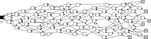
Let be the set of all directed acyclic graphs (also known as DAGs, that is, oriented graphs without cycles) with the following properties (see Figure 1).
-
•
The graph is finite and the multiplicity of any edge is at most two (i.e., there are at most two edges linking the same vertices).
-
•
There is a distinguished vertex such that for all , and . This vertex is called the genesis.
-
•
Any such that references ; that is, there is an oriented path666not necessarily unique from to .
We now describe the tangle as a continuous-time Markov process on the space . The state of the tangle at time is a DAG , where is the set of vertices and is the multiset of directed edges at time . The process’s dynamics are described in the following way:
-
•
The initial state of the process is defined by , .
-
•
The tangle grows with time, that is, and whenever .
-
•
For a fixed parameter , there is a Poisson process of incoming transactions; these transactions then become the vertices of the tangle.
-
•
Each incoming transaction chooses777the precise selection mechanism will be described below two vertices and (which, in general, may coincide), and we add the edges and . We say in this case that this new transaction was attached to and (equivalently, approves and ).
-
•
Specifically, if a new transaction arrived at time , then , and .
Let us write
for the “past” and the “future” with respect to (at time ). Note that these introduce a partial order structure on the tangle. Observe that, if is the time moment when was attached to the tangle, then for all . We also define the cumulative weight of the vertex at time by
| (1) |
that is, the cumulative weight of is one888its “own weight” plus the number of vertices that reference it. Observe that, for any , if approves then , and the inequality is strict if and only if there are vertices different from which also approve . Also note that the cumulative weight of any tip is equal to .
There is some data associated to each vertex (transaction), created at the moment when that transaction was attached to the tangle. The precise nature of that data is not relevant for the purposes of this paper, so we assume that it is an element of some (unspecified, but finite) set ; what is important, however, is that there is a natural way to say if the set of vertices is consistent with respect to the data they contain999one may think that the data refers to value transactions between accounts, and consistency means that no account has negative balance as a result, and/or the total balance has not increased. When it is necessary to emphasize that the vertices of contain some data, we consider the marked DAG to be , where is a function . We define to be the set of all marked DAGs , where .
A note on terminology: we reserve the term “node” for entities that participate in the system by issuing transactions (which are, by their turn, vertices of the tangle graph). That is, the “players” mentioned in Section 1 are nodes.
2.1 On attaching a new transaction to the Tangle
There is one very important detail that has not been explained, namely: how does a newly arrived transaction choose which two vertices in the tangle it will approve, i.e., what is the attachment strategy? Notice that, in principle, it would be good101010good in the sense described in Section 1 for the whole system if the new transactions always prefer to select tips as attachment places, since this way more transactions would be “confirmed”111111we discuss the exact meaning of this later; for now, think that “confirmed” means “referenced by many other transactions”. In any case, it is quite clear that the appropriate choice of the attachment strategy is essential for the correct functioning of the system, whatever this could mean.
It is also important to comment that the attachment strategy of a network node is something “internal” to it; what others can see, are the attachment choices of the node, but the mechanism behind them need not be publicly known. For this reason, an attachment strategy cannot be imposed in the protocol.
We now describe a possible choice of the attachment strategy, used to determine where the incoming transaction will be attached. It is also known as the recommended tip selection algorithm [20], since, due to reasons described above, the recommended nodes’ behavior is always to try to approve tips. We stress again, however, that approving only tips is not imposed in the protocol, since there is usually no way to know if a node “knew” if the transaction it approved was already approved by someone else before (also, there is no way to know which approving transaction was the first).
Let us denote by the set of all vertices that are tips at time , and let . To model the network propagation delays, we introduce a parameter , and assume that at time only is known to the entity that issued the incoming transaction. We then define the tip-selecting random walk, in the following way. It depends on a parameter (the backtracking probability) and on a function . The initial state of the random walk is the genesis 121212although in practical implementations one may start it in some place closer to the tips, and it is stopped upon hitting the set . It is important to observe that does not necessarily mean that is still a tip at time . Let be a monotone non-increasing function. The transition probabilities of the walkers are defined in the following way: the walk backtracks (i.e., jumps to a randomly chosen site it approves) with probability ; if approves , then the transition probability is proportional to , that is,
| (2) |
for we define the transition probabilities as above, but with . In words, the walker backtracks (i.e., moves one step away from the tips) with (total) probability , and advances one step towards the tips with (total) probability and relative weights as above. Note that the fact that guarantees that the random walk eventually reaches a tip131313more precisely, reaches a vertex that the node assumes to be a tip almost surely. In what follows, we will mostly assume that for some . We use the notation for the transition probabilities in this case. Intuitively, the smaller is the value of , the more random the walk is141414physicists would call the case of small high temperature regime, and the case of large low temperature regime (that is, stands for the inverse temperature). It is worth observing that the case and corresponds to the GHOST protocol of [23] (more precisely, to the obvious generalization of the GHOST protocol to the case when a tree is substituted by a DAG).
Now, to select two tips and where our transaction will be attached, just run two independent random walks as above, and stop when on the first hit . One can also require that should be different from ; for that, one may re-run the second random walk in the case its exit point happened to be the same as that of the first random walk. Observe that is a continuous-time transient Markov process on ; since the state space is quite large, it is difficult to analyse this process. In particular, for a fixed time , it is not easy to study the above random walk since it takes place on a random graph, e.g., can be viewed as a random walk in a random environment; it is common knowledge that random walks in random environments are notoriously hard to deal with.
Some motivation for choosing the attachment strategy in the above way is provided in [20]. Very briefly, it encourages the nodes to choose recent transactions for approval (since a transaction which approved a couple of old transactions, also known as lazy tip, is unlikely to be chosen by the above random walk, due to the large difference in cumulative weights in the argument of in (2)) and also gives protection against certain kinds of attacks (e.g., the double-spending attack).
Let be some number, typically close to . We say that a transaction is confirmed with confidence if, with probability at least , the large- random walk151515recall that the large- random walk is “more deterministic” ends in a tip which references that transaction. It may happen that a transaction does not get confirmed (even, possible, does not get approved a single time), and becomes orphaned forever. Let us define the event
We believe that the following statement holds true; however, we have only a heuristical argument in its favor, not a rigorous proof. In any case, it is mostly of theoretical interest, since, as explained below, in practice we will find ourselves in the situation where . We therefore state it as
Conjecture 2.1.
It holds that
| (3) |
Explanation..
First of all, it should be true that since is a tail event with respect to the natural filtration; however, it does not seem to be very easy to prove the 0–1 law in this context – recall that we are dealing with a transient Markov process on an infinite state space. Next, consider a tip which got attached to the tangle at time , and assume that it is still a tip at time ; also, assume that, among all tips, is “closest”, in some suitable sense, to the genesis.
Let us now think of the following question: what is the probability that will still be a tip at time ?
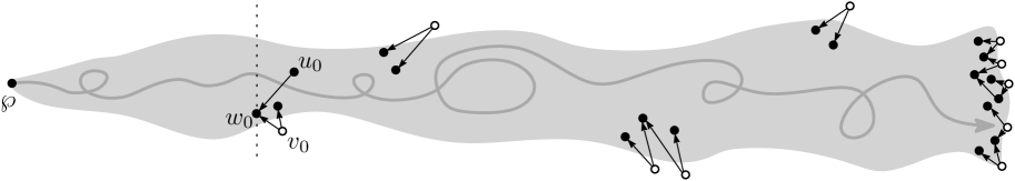
Look at Figure 2: during the time interval , new particles will arrive, and the corresponding walks will travel from the genesis looking for tips. Each of these walks will have to cross the dotted vertical segment on the picture, and with positive probability at least one of them will pass through , one of the vertices approved by . Assume that was already confirmed, i.e., it is connected to the right end of the tangle via some other transaction that approves . Then, it is clear (but not easy to prove!) that the cumulative weight of both and should be , and so, when in , the walk will jump to the tip with probability .
This suggests that the probability that (i.e., that still is tip at time ) is , and the Borel-Cantelli lemma161616to be precise, a bit more refined argument is needed since the corresponding events are not independent gives that the probability that will be eventually approved is less than or equal to depending on whether converges or diverges; the convergence (divergence) of the sum is equivalent to convergence (divergence) of the integral in (3) due to the monotonicity of the function . A standard probabilistic argument171717which is also not so easy to formalize in these circumstances would then imply that if the probability that a given tip remains orphaned forever is uniformly positive, then the probability that at least one tip remains orphaned forever is equal to . ∎
One may naturally think that it would be better to choose the function in such a way that, almost surely, every tip eventually gets confirmed. However, as explained in Section 4.1 of [20], there is a good reason to choose a rapidly decreasing function , because this defends the system against nodes’ misbehavior and attacks. The idea is then to assume that a transaction which did not get confirmed during a sufficiently long period of time is “unlucky”, and needs to be reattached181818in fact, the nodes of the network may adopt a rule that instructs to delete the transactions that are older than and still are tips from their databases to the tangle. Let us fix some : it stands for the time when an unlucky transaction is reissued (because there is already very little hope that it would be confirmed “naturally”). We call a transaction issued less than time units ago “unconfirmed”, and if a transaction was issued more than time units ago and was not confirmed, we call it “orphaned”. In the following, we assume that the system is stable, in the sense that the “recent” unconfirmed transactions do not accumulate and the time until a transaction is confirmed does not depend a lot on the moment when it appeared in the system191919simulations indicate that this is indeed the case when is small (cf. a recent paper [16]); however, it is not guaranteed to happen for large values of . We prefer not to elaborate on the exact mathematical definition of stability here, since it requires considering a certain compactification of the space of DAGs (which essentially amounts to considering DAGs with “genesis at minus infinity”), but, hopefully, the idea is intuitively clear anyway.
In that stable regime, let be the probability that a transaction is confirmed time units after it was issued for the first time; the number of times a transaction should be issued to achieve confirmation is then a Geometric random variable with parameter (and, therefore, with expected value ); so, the mean time until the transaction is confirmed is . Let us then recall the following remarkable fact belonging to the queuing theory, known as the Little’s formula (sometimes also referred to as the Little’s theorem or the Little’s identity):
Proposition 2.2.
Suppose that is the arrival rate, is the mean number of customers in the system, and is the mean time a customer spends in the system. Then .
Proof.
See e.g. Section 5.2 of [6]. To understand intuitively why this fact holds true, one may reason in the following way: assume that, while in the system, each customer pays money to the system with rate . Then, at large time , the total amount of money earned by the system would be (approximately) on one hand, and on the other hand. Dividing by and then sending to infinity, we obtain . ∎
Little’s formula then implies202020in the language of queuing systems, a reissued transaction is a customer which goes back to the server after an unsuccessful service attempt the following (recall that is the rate of the incoming transactions flow, not counting reattachments)
Proposition 2.3.
The average number of unconfirmed transactions212121we regard all reattachments as a single trasaction, and if one of the reattachments is confirmed, the transaction is considered confirmed in the system is equal to .
Proof.
Indeed, apply Proposition 2.2 with (think of a transaction which was reattached as a customer which returns to the server after an insuccessful service attempt; this way, the incoming flow of customers still has rate ). As observed before, the mean time spent by a customer in the system is equal to . ∎
When the tangle contains data, this, in principle, can make transactions incompatible between each other. In this case one may choose more sophisticated methods of tip selection. As we already mentioned222222recall the discussion around right after (2), selecting tips with larger values of provides better defense against attacks and misbehavior; however, smaller values of make the system more stable with respect to the transactions’ confirmation times. An example of “mixed-” strategy is the following. Define the “model tip” as a result of the random walk with large , then select two tips and with random walks with small , but check that
is consistent.
3 Selfish nodes and Nash equilibria
Now, we are going to study the situation when some participants of the network are “selfish” and want to use a customized attachment strategy, in order to improve the confirmation time of their transactions (possibly at the expense of the others).
For a finite set let us denote by the set of all probability measures on , that is
Let
be the union of the sets of all probability measures on the pairs of (not necessarily distinct) vertices of DAGs belonging to . Then, a general mixed attachment strategy is a map
| (4) |
with the property for any ; that is, for any with data attached to the vertices (which corresponds to the state of the tangle at a given time) there is a corresponding probability measure on the set of pairs of the vertices. Note also that in the above we considered ordered pairs of vertices, which, of course, does not restrict the generality.
Let be a fixed number. We now assume that, for a large , there are nodes that follow the default tip selection algorithm, and “selfish” nodes that try to minimize their “cost”, whatever it could mean232323for example, the cost may be the expected confirmation time of a transaction (conditioned that it is eventually confirmed), the probability that it was not approved during certain (fixed) time interval, etc.; below in (6) we provide the exact definition of the cost function we are working with in this paper. Assume that all nodes issue transactions with the same rate , independently. The overall rate of “honest” transactions in the system is then equal to , and the overall rate of transactions issued by selfish nodes equals . We also justify the assumption that the number of selfish nodes is large by observing that
-
•
a small number of nodes that do not want to disrupt the system but just want to obtain some advantages for themselves (like e.g. faster confirmations times) are unlikely to “globally” influence the system in any considerable way, even if they do obtain those advantages for themselves;
-
•
however, when it becomes known that it is possible to obtain advantages by deviating from the “recommended” behavior, it is reasonable to expect that a large number of independent entities would try to do it.
3.1 Some further assumptions and definitions
Let us now recall that, in practice, the nodes are computers running a specialized software, so they are selecting the places to attach their transactions in some algorithmic way, using limited physical resourses. In such situation, it is unrealistic to assume that a general strategy as in (4) could be implemented “directly”, since the space is infinite; for the same reason, even working with simple attachment strategies (which are maps that take an element of as an input and produce a deterministic pair of its vertices as an output) is unrealistic.
Therefore, it looks like a good idea to restrict the strategy space we are working with. First, we consider the following simplifying assumption (which is, by the way, also quite reasonable, since, in practice, one would hardly use the genesis as the starting vertex for the random walks due to runtime issues):
Assumption L. There is such that the attachment strategies of all nodes (including those that use the default attachment strategy) only depend on the restriction of the tangle to the last transactions that they see.
Observe that, under the above assumption, the set of all such strategies can be thought of as a compact convex subset of , where is sufficiently large.
In this section we use a different approach to model the network propagation delays: instead of assuming that an incoming transaction does not have information about the state of the tangle during last units of time, we rather assume that it does not have information about the last transactions attached to the tangle, where is some fixed positive number (so, effectively, the strategies would depend on subgraphs induced by transactions, although the results of this section do not rely on this assumption). Clearly, these two approaches are quite similar in spirit; however, the second one permits us to avoid certain technical difficulties related to randomness of the number of unseen transactions in the first case. Also, it will be more natural and convenient to pass from continuous to discrete time.
Now, even with the restrictions as above, it is still unrealistic to work with the simple strategies of the sort “choose a fixed pair of transactions for each possible restriction of the tangle to the set of last transactions”, because implementing it in practive would require effectively dealing with sets indexed by all possible restrictions, and the size of the latter set clearly grows exponentially in . Instead, as hinted in the beginning of this subsection, we think of different “attachment methods” as simple strategies. Formally, let be the set of all possible sub-DAGs of with vertices, and be the set of all probability measures on the vertices’ pairs of elements of . Clearly, the set is finite. An attachment method is then a map
it is thought of as a (randomized) polynomial-time polynomial-memory algorithm which takes the last transactions and returns a pair of those transactions which would serve as attachment’s locations. Then, the available simple strategies are attachment methods
where is some (unspecified) index set. It is also important to observe that this approach does not restricts generality. We then denote by the set of all mixed strategies of the form , where is a random variable on . Observe also that the set of simple strategies can be thought of as a subset of (which we assume also to be compact), where is sufficiently large, and would be then its convex hull.
Let be the attachment strategies used by the selfish nodes. To evaluate the “goodness” of a strategy, one has to choose and then optimize some suitable observable (that stands for the “cost”); as usual, there are several “reasonable” ways to do this. We decided to choose the following one, for definiteness and also for technical reasons (to guarantee the continuity of a certain function used below); one can probably extend our arguments to other reasonable cost functions. Assume that a transaction was attached to the tangle at time , so for all . Fix some (typically large) . Let be the moments when the subsequent (after ) transactions were attached to the tangle. For let be the event that the default tip-selecting walk242424i.e., the one used by nodes following the default attachment strategy on stops in a tip that does not reference . We then define the random variable
| (5) |
to be the number of times that the “subsequent” tip selection random walks do not reference (in the above, is the indicator function of an event ). Intuitively, the smaller is the value of , the bigger is the chance that is quickly confirmed.
Next, assume that are the transactions issued by the th (selfish) node. We define
| (6) |
to be the mean cost of the th node given that are the attachment strategies of the selfish nodes.
Definition 3.1.
We say that a set of strategies is a Nash equilibrium if
for any and any .
Observe that, since the nodes are indistinguishable, the fact that is a Nash equilibrium implies that so is for any permutation .
3.2 Main results
From now on, we assume that vertices contain no data, i.e., the set is empty; this is not absolutely necessary because, with the data, the proof will be essentially the same; however, the notations would become much more cumbersome. Also, there will be no reattachments; again, this would unnecessarily complicate the proofs (one would have to work with decorated Poisson processes). In fact, we are dealing with a so-called random-turn game here, see e.g. Chapter 9 of [15] for other examples.
Consider, for the moment, the situation when all nodes use the same attachment strategy (i.e., there are no selfish nodes). The restriction of the tangle on the last transactions then becomes a Markov chain on the state space . We now make the following technical assumption on that Markov chain:
Assumption D. The above Markov chain is irreducible and aperiodic.
It is important to observe that Assumption D is not guaranteed to hold for every natural attachment strategy; however, still, this is not a very restrictive assumption in practice because every finite Markov chain may be turned into an irreducible and aperiodic one by an arbitrarily small perturbation of the transition matrix.
Then, we are able to prove the following
Theorem 3.2.
Under Assumptions L and D, the system has at least one Nash equilibrium.
Symmetric games do not always have symmetric Nash equilibria, as shown in [9]. Also, even when such equilibria exist in the class of mixed strategies, they may be “inferior” to asymmetric pure equilibria; for example, this happens in the classical “Battle of the sexes” game (see e.g. Section 7.2 of [15]).
Now, the goal is to prove that, if the number of selfish nodes is large, then for any equilibrium state the costs of distinct nodes cannot be significantly different. Let us recall the notations we use: are the strategies of the selfish nodes, and , , are the mean costs of the selfish nodes, defined in (6). Now, we have the following
Theorem 3.3.
For any there exists (depending on the default attachment strategy) such that, for all and any Nash equilibrium it holds that
| (7) |
for all .
Now, let us define the notion of approximate Nash equilibrium:
Definition 3.4.
For a fixed , we say that a set of strategies is an -equilibrium if
for any and any .
The motivation for introducing this notion is that, if is very small, then, in practice, -equilibria are essentially indistinguishable from the “true” Nash equilibria.
Theorem 3.5.
For any there exists (depending on the default attachment strategy) such that, for all and any Nash equilibrium it holds that is an -equilibrium, where
| (8) |
(that is, all selfish nodes use the same “averaged” strategy defined above). The costs of all selfish nodes are then equal to
that is, the average cost in the Nash equilibrium.
In other words, for large one can essentially assume that all selfish nodes follow the same attachment strategy. This result will be important in Section 4, because it makes it possible to use (practical) simulations in order to find the Nash equilibria of systems with large number of selfish players.
3.3 Proofs
First, we need the following technical result:
Lemma 3.6.
Let be the transition matrix of an irreducible and aperiodic discrete-time Markov chain on a finite state space . Let be a continuous map from a compact set to the set of all stochastic matrices on (equipped by the distance inherited from the usual matrix norm on the space of all matrices on ). Fix , denote , and let be the (unique) stationary measure of . Then is also continuous (as a function of ).
Proof.
In the following we give a (rather) probabilistic proof of this fact via the Kac’s lemma, although, of course, a purely analytic proof is also possible. Irreducibility and aperiodicity of imply that, for some and
| (9) |
for all , where is the transition matrix in steps. Now, (9) implies that
| (10) |
for all and all .
Being a stochastic process on , let us define
(with the convention ) to be the hitting time of the site by the stochastic process . Now, let and be the probability and the expectation with respect to the Markov chain with transition matrix starting from . We now recall the Kac’s lemma (cf. e.g. Theorem 1.22 of [8]): for all it holds that
| (11) |
Now, (10) readily implies that, for all and ,
| (12) |
for some positive constants which do not depend on . This in its turn implies that the series
converges uniformly in and so is uniformly bounded from above252525and, of course, it is also bounded from below by ; also, the Uniform Limit Theorem (see e.g. Section D.6.2 of [19]) implies that is continuous in . Therefore, for any , (11) implies that is also a continuous function of . ∎
Proof of Theorem 3.2..
The authors were unable to find a result available in the literature that implies Theorem 3.2 directly; nevertheless, its proof is quite standard and essentially follows Nash’s original paper [18] (see also [10]). There is only one technical difficulty, which we intend to address via the above preparatory steps: one needs to prove the continuity of the cost function.
Denote by the invariant measure of the Markov chain given that the (selfish) nodes use the “strategy vector” . Then, the idea is to use Lemma 3.6 with , the transition matrix obtained from the default attachment strategy, and is the transition matrix obtained from the strategy (observe that nodes using the strategies , is the same as one node with strategy issuing transactions times faster). Assumption D together with Lemma 3.6 then imply that is a continuous function of .
Let be the expectation with respect to the following procedure: take the “starting” graph according to , then attach to it a transaction according to the strategy , and then keep attaching subsequent transactions according to the strategy (instead of and we may also use the strategy vectors; and would be then their averages). Let also be the random variable defined as in (5) for an arbitrary transaction issued by the th node. Then, the Ergodic Theorem for Markov chains (see e.g. Theorem 1.23 of [8]) implies that
| (13) |
It is not difficult to see that the above expression is a polynomial of the ’s coefficients (i.e., the corresponding probabilities) and -values, and hence it is a continuous function on the space of strategies . Using this, the rest of the proof is standard, it is obtained as a consequence of the Kakutani’s fixed point theorem [14], also with the help of the Berge’s Maximum Theorem (see e.g. Chapter E.3 of [19]). ∎
Proof of Theorem 3.3..
Without restricting generality we may assume that
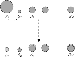
so we then need to proof that , where . Now, the main idea of the proof is the following: if is considerably larger than , then the owner of the first node may decide to adopt the strategy used by the second one. This would not necessarily decrease his costs to the former costs of the second node since a change in an individual strategy leads to changes in all costs; however, when is large, the effects of changing the strategy of only one node would be small, and (if the difference of and were not small) this would lead to a contradiction to the assumption that was a Nash equilibrium.
So, let us denote , the strategy vector after the first node adopted the strategy of its “more successful” colleague, see Figure 3.
Let
be the two “averaged” strategies. In the following, we are going to compare (the “old” cost of the second node) with (the “new” cost of the first node, after it adopted the second node’s strategy). We need the following
Lemma 3.7.
For any measure on and any strategy vectors and such that for all , we have
| (14) |
for all .
Proof.
Let us define the event
and observe that, by the union bound, the probability that it occurs is at most . Then, using the fact that (since, on , the first node does not “contribute” to ), write
where we also used that . This concludes the proof of Lemma 3.7. ∎
We continue proving Theorem 3.3. First, by symmetry, we have
| (15) |
Also, it holds that
| (16) |
by Lemma 3.7. Then, similarly to the proof of Theorem 3.2, we can obtain that the function
is continuous; since it is defined on a compact, it is also uniformly continuous. That is, for any there exist such that if , then
Choose . We then obtain from the above that
| (17) |
Proof of Theorem 3.5..
To begin, we observe that the proof of the second part is immediate, since, as already noted before, for an external observer, the situation where there are nodes with strategies is indistinguishable from the situation with one node with averaged strategy.
Now, we need to prove that, for any fixed it holds that
| (19) |
for all large enough (the claim would then follow by symmetry). Recall that we have
| (20) | ||||
| (21) | ||||
| and | ||||
| (22) | ||||
where
4 Simulations
In this section we investigate Nash equilibria between selfish nodes via simulations. As discussed in Section 1, this is motivated by the following important question: since the choice of an attachment strategy is not enforced, there may indeed be nodes which would prefer to “optimise” their strategies in order to decrease the mean confirmation time of their transactions. So, can this lead to a situation where the corresponding Nash equilibrium is “bad for everybody”, effectively leading to the system’s malfunctioning?
Due to Theorem 3.5 we may assume that all selfish nodes use the same attachment strategy. Even then, it is probably unfeasible to calculate that strategy exactly; instead, we resort to simulations, which indeed will show that the equilibrium strategy of the selfish nodes will not be much different from the (suitably chosen) default strategy, at least in the (very natural) situation below. But, before doing that, let us explain the intuition behind this fact. Naively, a reasonable strategy for a selfish node would be the following:
-
(1)
Calculate the exit distribution of the tip-selecting random walk.
-
(2)
Find the two tips where this distribution attains its “best”272727i.e., the maximum and the second-to-maximum values.
-
(3)
Approve these two tips.
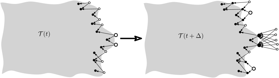
However, this strategy fails when other selfish nodes are present. To understand this, look at Figure 4: many selfish nodes attach their transactions to the two “best” tips. As a result, the “neighborhood” of these two tips becomes “overcrowded”: there is so much competition between the transactions issued by the selfish nodes, that the chances of them being approved soon actually decrease282828the “new” best tips are not among them, as shown on Figure 4 on the right.
To illustrate this fact, several simulations have been done. All the results depicted here were generated using (2) as the transition probabilities, with , and a network delay of second. Also, a transaction will be reattached if the two following criteria are met:
-
(1)
the transaction is older than 20 seconds
-
(2)
the transaction is not referenced by the tip selected by a random walk with 292929here, when the random walk must choose among transactions with the same weight, it will choose randomly, with equal probabilities.
This way, we guarantee not only that the unconfirmed transactions will be eventually confirmed, but also that all transactions that were never reattached are referenced by most of the tips. Note that when the reattachment is allowed in the simulations, if a new transaction references an old, already reattached transaction together with its newly reissued counterpart, there will be a double spending. Even though the odds of that are low (since when a transaction is re-emitted, it will be old enough to be almost never chosen by the random walk algorithm), a specific procedure was included in the simulations in order to not allow double spendings.
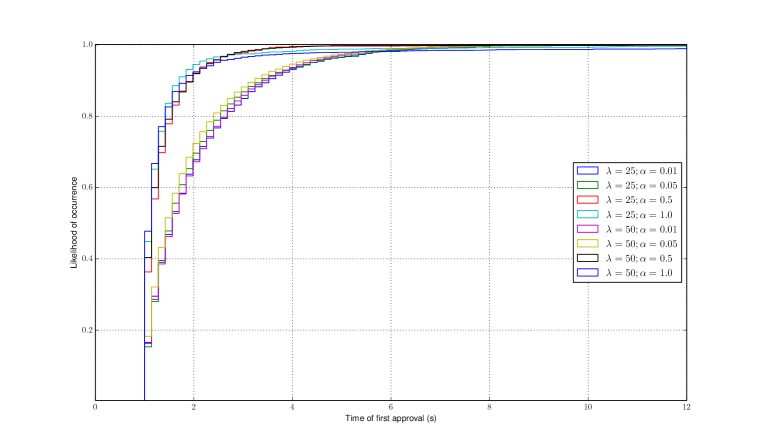
The average costs were simulated as defined at equations (5) and (6), so a certain value of had to be chosen. Since the value of is related to the time of approval of (whenever the transaction is indeed approved before ), we want to be sufficiently large, in order to capture the effect of most of the approvals. Figure 5 depicts the typical cumulative distribution of the time of the first approval, for several values of and . Note that roughly 95 of the transactions will be approved before s, and almost its totality will be approved before s. For that reason, in both cases ( and ), the mean cost was calculated over the transactions attached during a time interval of approximately 10s ( for and for ), so almost the totality of approvals will be “seen” by the average cost.
4.1 One dimensional Nash equilibria
In this section, we will study the Nash equilibria of the tangle problem, considering the following strategy space:
where the simple strategies and are the default tip selection strategy and the “greedy” strategy (defined in the beginning of this section) correspondingly; that is, where , . The goal is to find the Nash equilibria relative to the costs defined in the last section (equations (6) and (5)). The selfish nodes will try to optimise their transaction cost with respect to .
By Theorem 3.5, each Nash equilibrium in this form will be equivalent to another Nash equilibrium with “averaged” strategies, i.e.:
Now, suppose that we have a fixed fraction of selfish nodes, that choose a strategy among the possible . The non-selfish nodes will not be able to choose their strategy, so they will be restricted, as expected, to . Note that, since they cannot choose their strategy, they will not “play” the game. Since the costs are linear over , such mixed strategy game will be equivalent303030this way, we deal with just one variable () instead of two ( and ) and none of the parameters of the system is lost to a game where only a fraction of the nodes chooses over , and the rest of the nodes chooses over . Note that this equivalence does not contradict the theorems proved in the last sections, that state:
-
•
all the nodes will have the same average costs when the system is at a Nash equilibrium;
-
•
any Nash equilibrium has an equivalent Nash equilibrium with “averaged” strategies, where all the nodes will have the same strategies.
From now on, we will refer (unless stated otherwise) to this second pure strategy game. Figure 6(a) represents a typical graph of average costs of transactions issued under and , as a function of the fraction , for a low and two different values of . As already demonstrated, when in equilibrium, the selfish nodes should issue transactions with the same average costs. That means that the system should reach equilibrium in one of the following states:
-
(1)
some selfish nodes choose and the rest choose (), all of them with the same average costs;
-
(2)
all selfish nodes choose ();
-
(3)
all selfish nodes choose ().
(a) (b)
If the two curves on the graphs do not intersect, the equilibrium should be clearly at state (2) or (3), depending on which of the average costs is larger. If the two curves on the graphs intercept each other, we will also have the intersection point as a Nash equilibrium candidate. We call the vector of strategies on equilibrium and the fraction of nodes that will issue transactions under when the system is in . We define and , meaning that and will be deviations from , that result from one node switching strategies, from to and from to , respectively. We also define and as strategy vectors related to and . Note on Figure 7 that this kind of Nash equilibrium candidate may not be a real equilibrium. In the first example (7(a)), when the system is at point and a node switches strategies from to (moving from to ), the cost actually decreases, so cannot be a Nash equilibrium. On the other hand, the second example (7(b)) shows a Nash equilibrium at point , since deviations to and will increase costs.
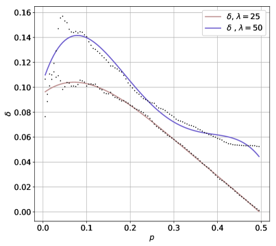
Now, let us re-examine Figure 6(a). Here, the Nash equilibrium will occur at the point , since we have a situation as on Figure 7(b). That point is easily found at Figure 6(b), when . Note that the Nash equilibrium for a larger will be at a smaller than the Nash equilibrium for a smaller . This was already expected, since, for a larger , the tips will be naturally more “overcrowded”, so the effect depicted at Figure 4 will be amplified. Thus, the Nash equilibrium for the higher cases must occur with a smaller proportion of transactions issued with the pure strategy .
Let us now again consider the mixed strategy game. In the case when all the nodes are allowed to choose between the two pure strategies ( and ), the Nash equilibrium will be indeed at (as expected, since in this case ). If just a fraction of the nodes is selfish, then the Nash equilibrium will occur when . Now, if , the costs of the nodes will not coincide313131that is the case for the range of studied parameters. In that case, the average cost of transactions under will always be smaller than the average cost of transactions under , meaning that the Nash equilibrium will be met at . Summing up, the Nash equilibrium , in these cases, will be met at:
(a) (b)
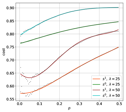
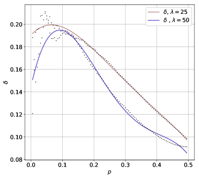
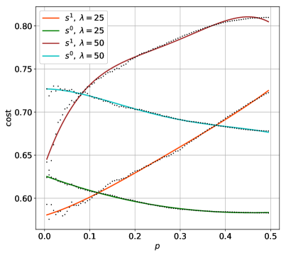
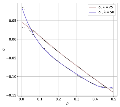
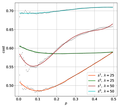
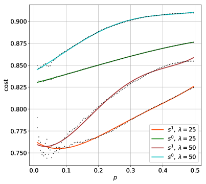
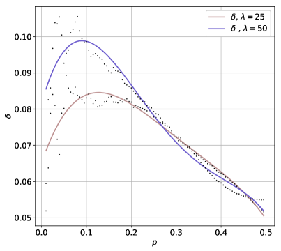
Figure 8(a) represents a typical graph of average costs of transactions under and transactions under as a function of fraction , for a higher . In that case, even though the average costs of transactions under and transactions under do not coincide for any reasonable (meaning that, here, the Nash equilibrium will be met at ), the typical difference between the possible pure strategies (that, from now on, we will call absolute gains) will be low, as depicted on Figure 8(b).
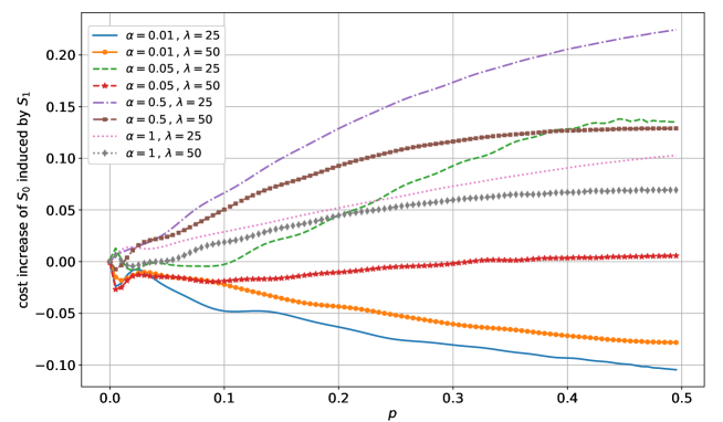
Figure 9 shows the average cost increase imposed on the nodes following the default strategy by the nodes issuing transactions under . Let be the non-greedy nodes costs depicted in Figure 8(a). The cost increase is calculated as , so it will be the relative difference of the cost of a non-selfish node in the presence of a fraction of selfish transactions and the cost of a non-selfish node when there are no selfish transactions at all. This difference is low, meaning that the presence of selfish nodes do not harm the efficiency of the non-selfish nodes. Note that this difference is small for all reasonable values of , but even for the larger simulated values of , the difference is still less than 25%. An interesting phenomenon, as shown in the same graph, is that the average cost increase imposed on the non-greedy nodes may actually be negative. For low values of , just a small fraction of the transactions under will share the approved tips with the transactions under . This fraction of transactions will approve overcrowded tips, and will have their costs increased. All the other transactions under will have their sites less crowded, since an increase in will mean a decrease in competition over these transactions. Finally, on average, the honest nodes will have their costs decreased.
(a) (b)
(a) (b)
5 Conclusions and future work
In the first part of this paper, we prove the existence of (“almost symmetric”) Nash equilibria for a game in the tangle where a part of players tries to optimise their attachment strategies. In the second part of the paper, we numerically determine, for a simple space strategy and some range of parameters, where these equilibria are located.
Our results show that the studied selfish strategy outperform the non-selfish ones by a reasonable order of magnitude. The data show a 25% (in the most extreme scenario) difference in the nodes gains, which in some situations, may be large enough. Nevertheless, the computational cost of a selfish strategy is intrinsically larger than the computational cost of the non-selfish strategies, since the selfish strategy uses the probability distribution of the tips, which is costly to calculate for a random walk with backtracking. They will also have to monitor the tangle, to know its parameters (like , etc) and act accordingly. Also, even a extreme scenario, where almost half of the transactions were issued by a selfish node, is not enough to harm the non-selfish ones in a meaningful way.
On the other hand, our results raise further questions. The obtained data exhibit a deep qualitative dependence on the parameter of the simulation. This parameter is related to the randomness of the random walk: a low implies a high randomness; a higher implies a low randomness, meaning that the walk will be almost deterministic. Further simulations will be done in order to study the effect of that variable in the equilibria. Also, we only studied equilibria for a given cost, relative to the probability of confirmation of the transactions in a certain interval of time. Since this probability depends heavily on the interval of time chosen (because the probability distribution of the confirmations is far from uniform), another time intervals, that will have another practical meaning, must be analysed.
Finally, the equilibrium in the multidimensional strategy space should be studied in a more quantitative and analytic way, since it should depend strongly on and ; and until now it was studied in just a narrow range of parameters. Further research will also be done in order to optimise the default tip selection strategy in a way that minimises this cost imposed by the selfish strategies. Through implementing research methods and techniques from the cross-reactive fields of measure theory, game theory, and graph theory, progress towards resolving the tangle-related open problems has been well under way and will continue to be under investigation.
As already mentioned, in this paper we consider only “selfish” players, i.e., those who only care about their own costs but still want to use the network in a legitimate way. We do not consider at all the case when there are “malicious” ones, i.e., those who want to disrupt the network even at a cost to themselves. We are going to treat several types of attacks against the network in the subsequent papers. Some preview of this ongoing work is available in [21].
Acknowledgements
The authors thank Alon Gal, Gur Huberman, Bartosz Kumierz, John Licciardello, Andreas Penzkofer, Samuel Reid, and Clara Shikhelman for valuable comments and suggestions. The authors are also grateful to the anonymous reviewers for carefully reading the first version of this paper and providing valuable comments and suggestions.
References
- [1] http://www.iota.org/
-
[2]
Baird, L. (2016).
The Swirlds hashgraph consensus algorithm: fair,
fast, Byzantine fault tolerance.
http://www.swirlds.com/downloads/SWIRLDS-TR-2016-01.pdf - [3] Churyumov, A. (2016). Byteball: a decentralized system for storage and transfer of value. https://byteball.org/Byteball.pdf
- [4] Cooper, C., Frieze, A. (2007). The cover time of the preferential attachment graph. J. Comb. Theory B 97 (2), 269–290.
- [5] Cooper, C., Frieze, A., Pett, S. (2017). The covertime of a biased random walk on . arXiv:1708.04908
- [6] Cooper, R.B. (1981). Introduction to Queueing Theory (2nd ed.). North Holland.
- [7] Doyle, P.G., Snell, J.L. (1984). Random walks and electric networks. Carus Mathematical Monographs 22, Mathematical Association of America, Washington.
- [8] Durrett, R. (2012). Essentials of Stochastic Processes (2nd. ed.) Springer.
- [9] Fey, M. (2012). Symmetric games with only asymmetric equilibria. Games Econ. Behavior 75 (1), 424–427.
- [10] Fink, A.M. (1964). Equilibrium in a stochastic -person game. J. Sci. Hiroshima Univ. Ser. A-I Math. 28 (1), 89–93.
- [11] Frieze, A., Krivelevich, M., Michaeli, P., Peled, R. (2017). On the trace of random walks on random graphs. arXiv:1508.07355
- [12] Iacobelli, G., Figueiredo, D.R., Neglia, G. (2017). Transient and slim versus recurrent and fat: random walks and the trees they grow. arXiv:1711.02913
- [13] Jerison, D., Levine, L., Sheffield, S. (2014). Internal DLA and the Gaussian free field. Duke Math. J. 163 (2), 267–308.
- [14] Kakutani, S. (1941). A generalization of Brouwer’s fixed point theorem. Duke Math. J. 8 (3), 457–459.
- [15] Karlin, A.R., Peres, Y. (2017). Game Theory, Alive. American Mathematical Society.
-
[16]
Kuśmierz, B., Gal, A. (2018).
Probability of being left behind and probability of becoming
permanent tip in the Tangle.
https://www.iota.org/research/academic-papers -
[17]
Lerner, S.D. (2015).
DagCoin: a cryptocurrency without blocks.
https://bitslog.wordpress.com/2015/09/11/dagcoin/ - [18] Nash, J.F. (1950). Equilibrium points in -person games. Proc. Natl. Acad. Sci. 36 (1), 48–49.
- [19] Ok, E.A. (2007). Real Analysis with Economics Applications. Princeton University Press.
- [20] Popov, S. (2015). The tangle. https://iota.org/IOTAWhitepaper.pdf
-
[21]
Popov, S. (2018).
Local modifiers in the Tangle.
https://www.iota.org/research/academic-papers -
[22]
Sompolinsky, Y., Lewenberg, Y., Zohar, A.
(2016).
SPECTRE:
Serialization of proof-of-work events: confirming transactions via
recursive elections.
https://eprint.iacr.org/2016/1159.pdf - [23] Sompolinsky, Y., Zohar, A. (2013). Secure high-rate transaction processing in Bitcoin. https://eprint.iacr.org/2013/881.pdf