Simulation of low-depth quantum circuits as complex undirected graphical models

Abstract

Near term quantum computers with a high quantity (around 50) and quality (around 0.995 fidelity for two-qubit gates) of qubits will approximately sample from certain probability distributions beyond the capabilities of known classical algorithms on state-of-the-art computers, achieving the first milestone of so-called quantum supremacy. This has stimulated recent progress in classical algorithms to simulate quantum circuits. Classical simulations are also necessary to approximate the fidelity of multiqubit quantum computers using cross entropy benchmarking. Here we present numerical results of a novel classical simulation algorithm to calculate output probabilities of universal random circuits with more qubits and depth than previously reported. For example, circuits with $5\times 9$ qubits of depth 40, $7\times 8$ qubits of depth 30, and $10\times(\kappa>10)$) qubits of depth 19 are all easy to sample by calculating around one thousand measurements in a single workstation. Cross entropy benchmarking with around one million measurements for these circuits is now also possible in a computer cluster. The algorithm is related to the “Feynman path” method to simulate quantum circuits. For low-depth circuits, the algorithm scales exponentially in the depth times the smaller lateral dimension, or the treewidth, as explained in Boixo et. al. Boixo et al. (2016), and therefore confirms the bounds in that paper. In particular, circuits with $7\times 7$ qubits and depth 40 remain currently out of reach. Follow up work on a supercomputer environment will tighten this bound.

I Introduction

Quantum computers offer the promise to perform a number of computational tasks believed to be impossible for classical computers. Prominent examples are quantum simulations Feynman (1982); Aspuru-Guzik et al. (2005); Hastings et al. (2015); Wecker et al. (2015); O’Malley et al. (2016); Reiher et al. (2017); Babbush et al. (2017); Jiang et al. (2017) and factoring large numbers Shor (1999). Given the progress in classical computation, surpassing the capabilities of state-of-the-art algorithms and computers is no small feat. Therefore, in the path to more practical “quantum supremacy” breakthroughs, it is reasonable to focus first on more specific milestones better suited for near-term quantum computers with a high quantity (around 50) and quality (around 0.995 two qubit gate fidelity) of qubits. Sampling from the output distribution of certain families of quantum circuits has been identified as a promising venue for a first milestone of quantum supremacy Aaronson and Arkhipov (2011); Bremner et al. (2016a, b); Gao et al. (2017); Hangleiter et al. (2017); Kapourniotis and Datta (2017). Universal random circuits Boixo et al. (2016) (or more general chaotic quantum evolutions Neill et al. (2017)) are particularly well-suited for near term devices. On the one hand, we note that an important characteristic of these types of sampling problems is that they are hypersensitive to perturbations Schack and Caves (1993); Scott et al. (2006) and, therefore, approximate classical algorithms are unlikely to work. On the other hand, this also implies that an experimental implementation will not be successful unless the qubits being used are very coherent and all operations have high fidelity (and very fine-tuned control). Nevertheless, the same hypersensitivity to perturbations makes this type of demonstration of quantum supremacy a good benchmark for multiqubit fidelity of universal computers using cross entropy benchmarking Boixo et al. (2016); Neill et al. (2017). A successful implementation of a first milestone of quantum supremacy would demonstrate the basic building blocks for a large-scale quantum computer within the operational range of the surface code Barends et al. (2014); Fowler et al. (2012).

The prospect of a near-term demonstration of quantum supremacy has also stimulated recent progress in classical algorithms to simulate quantum circuits De Raedt et al. (2007); Boixo et al. (2016); Zulehner and Wille (2017); Häner and Steiger (2017); Pednault et al. (2017). The most efficient algorithms previously reported to simulate generic circuits (without symmetries that allow for faster compressions Viamontes et al. (2009); Zulehner and Wille (2017) or “emulations”) apply gates to a vector state, implemented as highly optimized matrix-vector multiplications De Raedt et al. (2007); Boixo et al. (2016); Häner and Steiger (2017); Pednault et al. (2017). Benchmarking results for a highly optimized algorithm of this type were reported in Ref. Boixo et al. (2016) for $6\times 7$ qubits and depth 27 taking 989 seconds and performed in the Edison supercomputer. More recently, Ref. Häner and Steiger (2017) reported a simulation using 8192 nodes and 0.5 petabytes of memory for a quantum circuit (in the same ensemble) with $5\times 9$ qubits and depth 25 on the new Cori II supercomputer in 552 seconds (and $6\times 7$ qubits in 80 seconds). Finally, Ref. Pednault et al. (2017) recently reported simulations of a circuit with $7\times 7$ qubits and depth 27 and another circuit of $7\times 8$ qubits and depth 23, along two days in the IBM Blue Gene/Q supercomputer. Computing time in a supercomputer at that scale is scarce and expensive.

We generalize the simulation of a quantum circuit by mapping it onto an undirected graphical model, which we compute using the variable elimination algorithm, developed in the context of exact inference Dechter (1998); Murphy (2012, 2012). In some cases a circuit amplitude can be mapped directly to the partition function of an Ising model with imaginary temperature Boixo et al. (2016), which can be computed exactly with the same method. This is related to the Feynman path method Bernstein and Vazirani (1997), the tensor network method Markov and Shi (2008), and similar approaches Aaronson and Chen (2016). The algorithm is explained in Sec. IV, and we provide pseudocode in App. A. We are mostly interested in sampling output probabilities, but the same method can be used to calculate many amplitudes at once or calculating observables exactly. The quantum circuits implemented with superconducting qubits, which is our main focus, use controlled-phase gates (and controlled-Z gates in particular) as the predominant two-qubit gate Martinis and Geller (2014); Barends et al. (2014). We exploit the fact that controlled-phase gates are diagonal in the computational basis (this is also used in the algorithms referred above). The cost of this algorithm is exponential in $\min(O(d\ell),O(n))$ for depth $d$, minimum lateral dimension $\ell$ and total number of qubits $n$. More optimally, the cost is exponential in the treewidth, which is upper bounded by $\min(O(d\ell),O(n))$, and was estimated in Ref. Boixo et al. (2016) (see also Sec. IV.2).

II Numerical results

In the simplest implementation, we compute one-by-one the exact probabilities assigned by a quantum circuit ${\mathcal{U}}$ to a chosen set of outputs. One use case is cross entropy benchmarking Boixo et al. (2016); Neill et al. (2017), where we need to compute the probabilities assigned by ${\mathcal{U}}$ to the bit-strings measured in an experiment, see App. B. In other use cases, such as estimating the value of an observable, or simulating sampling from the output distribution, the error scales as $t^{-1/2}$, where $t$ is the number of output probabilities computed (see App. C). If the time per amplitude is small enough (for instance, around 100 seconds or less), then we can obtain enough probabilities in a single workstation in a reasonable time (for instance, 1000 probabilities in around one day). The sampling is also trivially parallelizable across machines. The algorithm can be modified to sample sets of probabilities in a single run, see Eq. (6). It can also be modified to calculate an observable exactly, but the computational cost might change. This algorithm is not useful in all cases. For instance, Ref. Boixo et al. (2016) numerically verified that the output distribution of low-depth universal random circuits approaches the entropy of the Porter-Thomas (or exponential) distribution to within its standard deviation of order $2^{-n/2}$. It would require to compute a number of output probabilities of order $2^{n}$ to verify this property. We also note that for enough depth a direct evolution of the wave vector is likely to become more efficient, as it is easier to optimize.

In what follows we report the time per probability (or amplitude) in a single workstation. We use as a reference a machine with 2$\times$ 14-core Intel E5-2690 V4 processors @ 2.6GHz, 35MB Cache and 128GB DDR4 2400MHz RAM. We use single precision complex numbers, as the relative error per probability is negligible for the sizes computed (less then $10^{-5}$). The computation of a single probability can also be distributed among several machines as the size of the computation grows. We leave this and other optimizations (such as reusing part of the computation when calculating many probabilities) for follow up work.

We are interested in circuits in a 2D lattice, as they are available experimentally Martinis and Geller (2014); Barends et al. (2014). We will use the following set of gates:

1. We use controlled-phase (CZ) gates as two-qubit gates.

2. For a concrete example we use single qubit gates in the set $\{{\rm H},{\rm X}^{1/2},{\rm Y}^{1/2},{\rm T}\}$. The gate ${\rm H}$ is a Hadamard, ${\rm X}^{1/2}$ (${\rm Y}^{1/2}$) is a $\pi/2$ rotation around the ${\rm X}$ (${\rm Y}$) axis of the Bloch sphere, and the non-Clifford T gate is the diagonal matrix $\{1,e^{i\pi/4}\}$.

We use the rules for the layout of gates described in Boixo et al. (2016). We are also particularly interested in superconducting qubits, and it is currently not possible to perform two CZ gates simultaneously in two neighboring qubits Barends et al. (2014, 2015); Kelly et al. (2015); Barends et al. (2016). This restriction was used for the circuits.

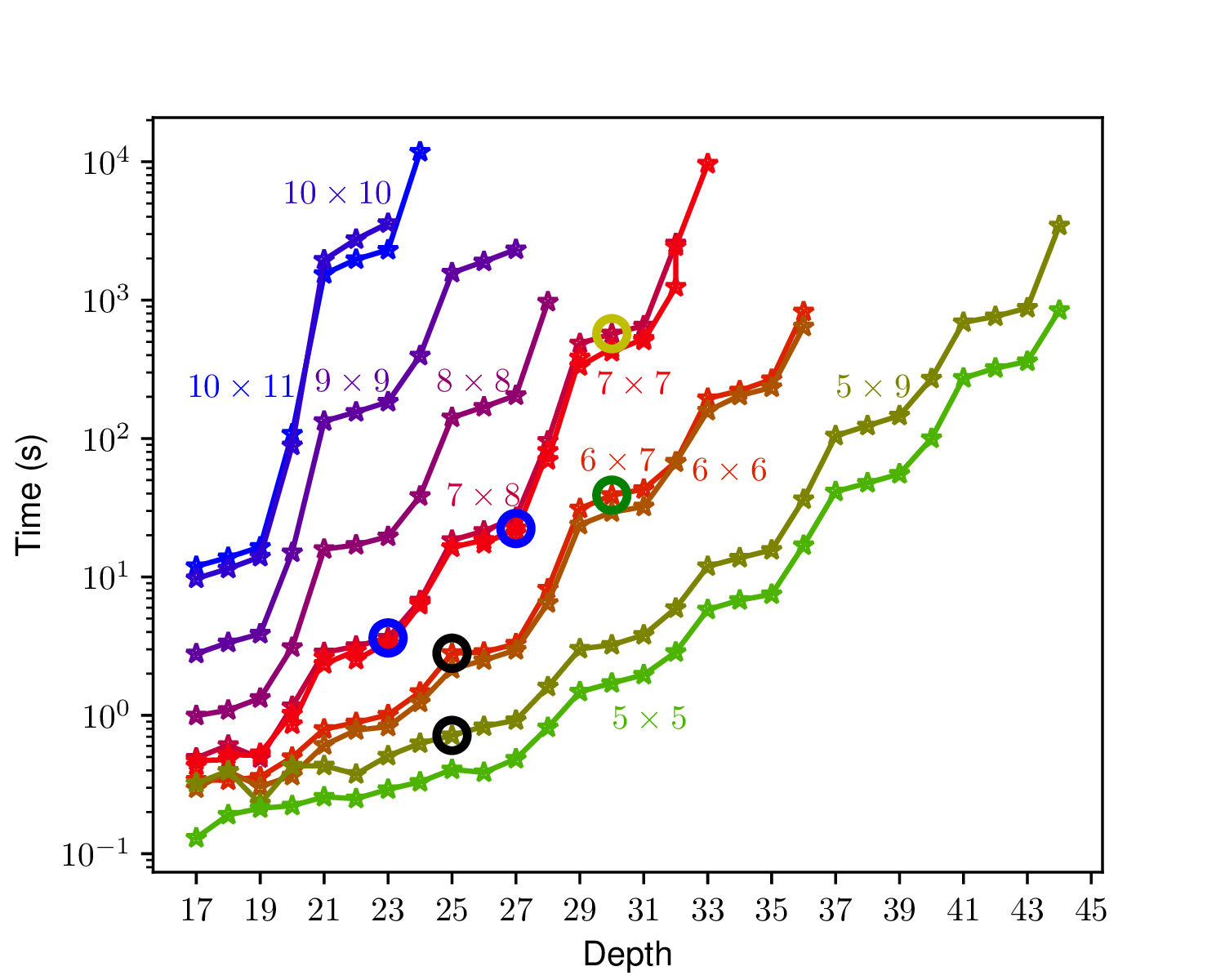
Figure 1: Time per output probability for a typical instance as a function of depth on a single workstation, using TensorFlow as the engine for the computation and a vertical elimination ordering (see Sec. IV.1). Different colors corresponds to different circuit sizes, from $5\times 5$ (and $5\times 9$) qubits, to $10\times 10$ ($10\times 11$). The green circle marker corresponds to the circuits simulated in Ref. Boixo et al. (2016), black circles to Ref. Häner and Steiger (2017), and blue circles to Ref. Pednault et al. (2017). The yellow circle is the circuit used in Fig. 3.

Figure 1 shows the time per output probability for typical instances of different circuit sizes as a function of depth on a single workstation. Different colors correspond to different circuit sizes, from $5\times 5$ (and $5\times 9$) qubits, to $10\times 10$ ($10\times 11$). Here we use a vertical variable elimination ordering, which in essence processes the “Feynman path” or worldline of each qubit in sequence (see Sec. IV.1). The processing time (and required memory) of each computation grows exponentially with depth. The exponential growth is also faster for larger circuits. More specifically, we process the worldline of the qubits ordered first along the smaller lateral dimension $\ell$. The cost of computing probabilities for circuits with $5\times 9$ qubits, with $\ell=5$, is similar to the cost of circuits with $5\times 5$ qubits. The same is true for circuits of sizes $7\times 7$ and $7\times 8$ with $\ell=7$, and also sizes $10\times 10$ and $10\times 11$ (or larger) with $\ell=10$. In this implementation the computational graph of the algorithm was constructed in python and processed with TensorFlow version 1.3.0 Abadi et al. (2016). For each size depicted, the computation becomes memory limited (128 GB RAM) after the highest depth shown (depths around $31$ to $33$ for $7\times 7$ qubits depending on the instance).

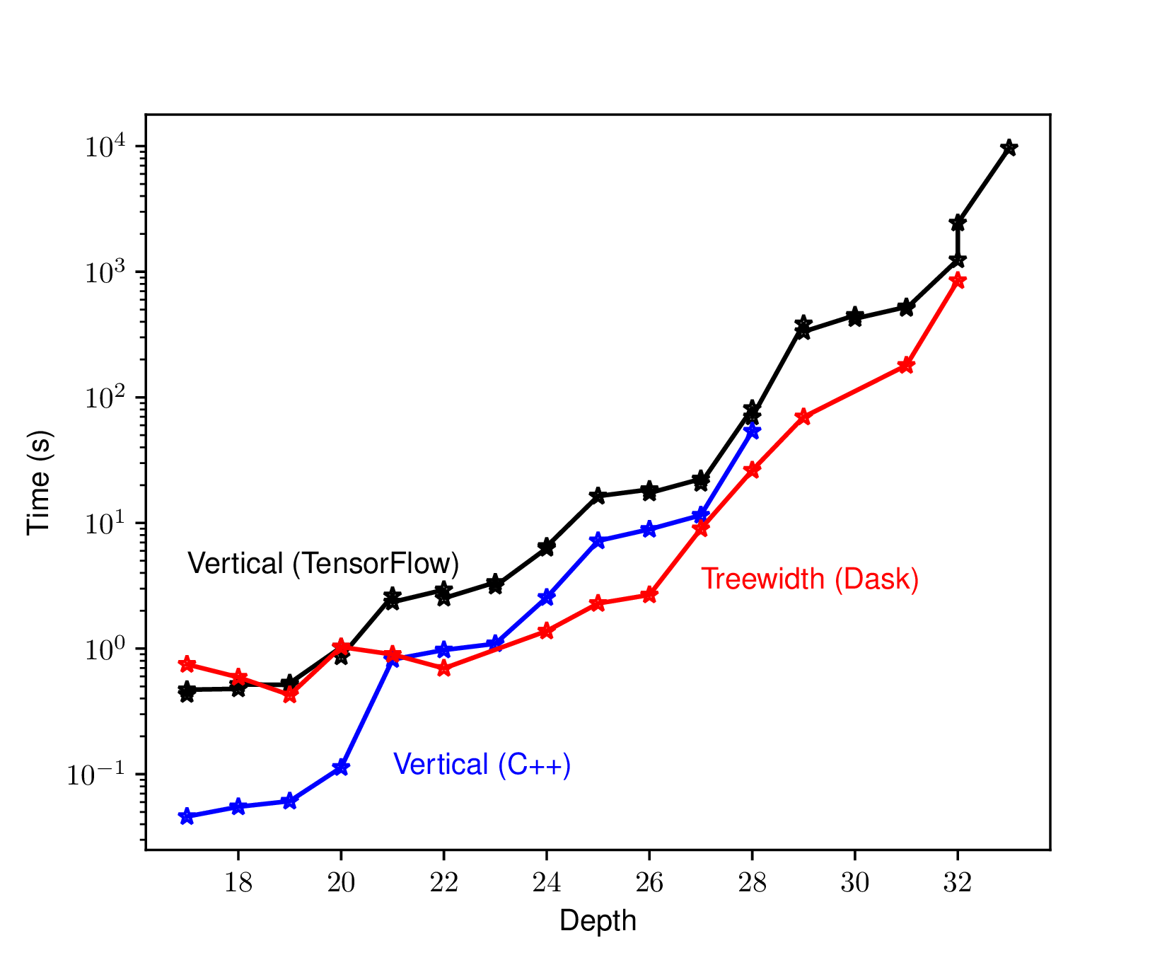
Figure 2: Timings per output probability for typical instances at different depths using different implementations of the graphical model variable elimination algorithm. We compare a TensorFlow implementation and a C++ implementation using the vertical variable elimination ordering (see Sec. IV.1), and an implementation using the Dask python package using a variable ordering obtained by running QuickBB Gogate and Dechter (2004) for a day to find a treewidth decomposition at each depth (see Sec. IV.2).

Figure 2 compares the run times per output probability as a function of depth for three different implementations. One is the implementation with a TensorFlow Abadi et al. (2016) backend using the same vertical variable elimination ordering as in Fig. 1. This implementation is efficient and portable to the different architectures in which TensorFlow is available, including distributed environments. A second implementation is a native C++ implementation. The C++ implementation is faster, although the run times are similar, and is probably less portable and harder to distribute across machines. Finally we also show an implementation using a variable ordering obtained by running QuickBB Gogate and Dechter (2004) for a day to find a treewidth decomposition at each depth. The tensors obtained by this variable elimination ordering are worse aligned than in the vertical ordering, and can not be processed by the off-the-shelf TensorFlow binary. Therefore we used the python module Dask Das in this case (Dask was slower than TensorFlow in the vertical ordering for our current implementation). Not taking into account the time required to find a better variable elimination ordering, the treewidth ordering is faster. In all three cases further optimizations are possible, and the run times reported are merely indicative. All three implementations are memory (RAM) limited after the last depth shown in the figure.

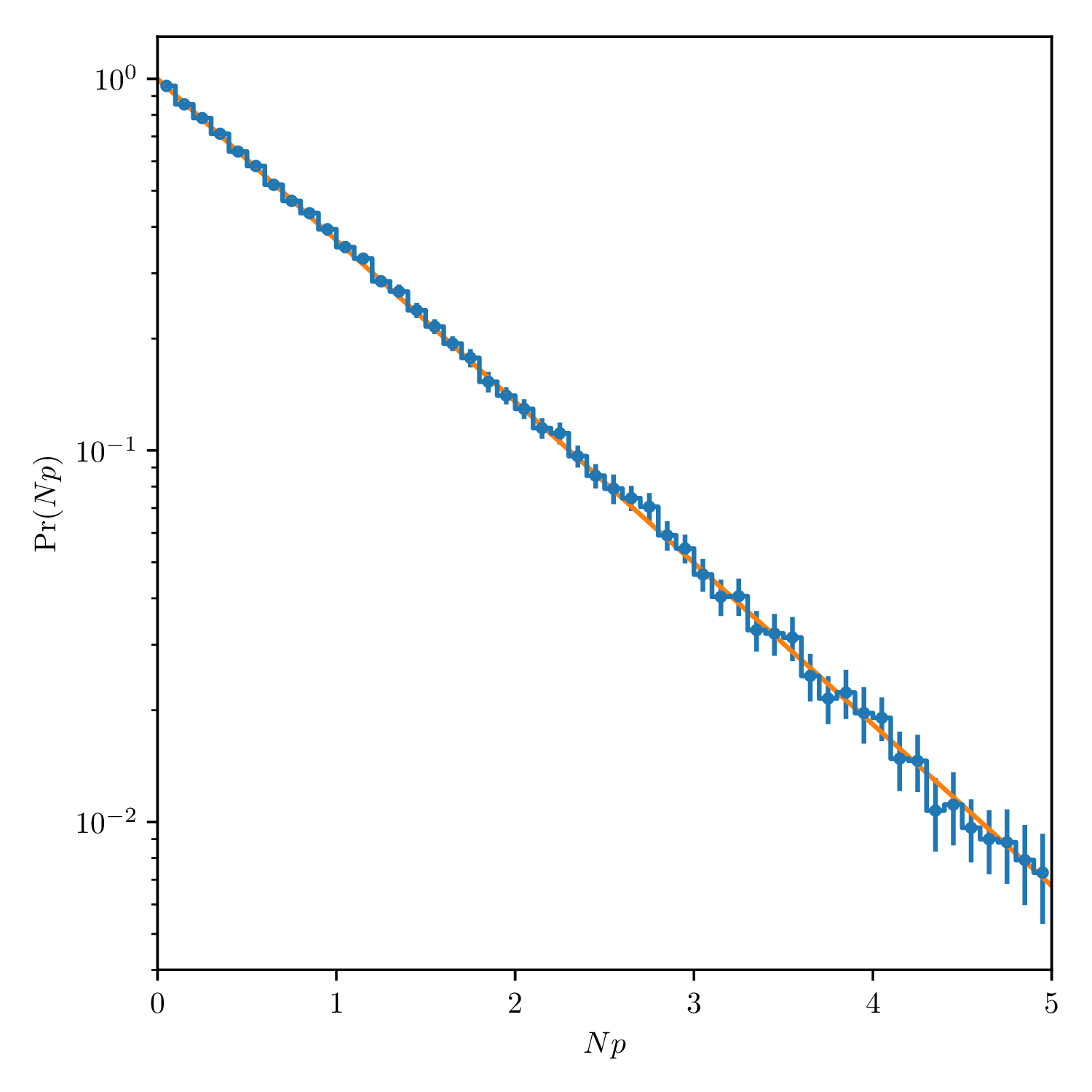
Figure 3: Histogram (blue) of the output probabilities for a circuit with $7\times 8$ qubits and depth 30. We calculated 200 thousand exact probabilities. Error bars were obtained by bootstrapping. We see that the probabilities obey the exponential or Porter-Thomas distribution (red) Boixo et al. (2016).

As an illustration, we calculated 200 thousand output probabilities of a universal random circuit with $7\times 8$ qubits and depth 30. We show in Fig. 3 that the distribution obeys the exponential or Porter-Thomas distribution. We also used these probabilities to estimate the entropy of the output distribution of this circuit. We obtain an entropy of $\log(2^{7\times 8})-0.422\pm 0.007$, while the analytical value for a Porter-Thomas distribution is $\log(2^{7\times 8})-0.4228$ Boixo et al. (2016).

III Circuit simulation as an undirected graphical model

The basic principle of the algorithm can be seen as a mapping of a quantum circuit to an undirected graphical model with complex factors. This is equivalent to the interaction graph of the Ising model detailed in Ref. Boixo et al. (2016). The evaluation is carried out using an algorithm developed in the context of exact inference for undirected graphical models Dechter (1998); Murphy (2012); Bishop and ligne) (2006), but in the present case the factors are complex. A similar algorithm was used to find an exact ground state of a classical Ising model in Boixo et al. (2014). We now explain in detail how the undirected graphical model is constructed.

III.1 Feynman path method

We represent a quantum circuit by a product of unitary matrices $U^{(t)}$ corresponding to different clock cycles $t$. We introduce the following notation for the amplitude of a particular bit-string after the final cycle of the circuit,

$$\langle x|{\mathcal{U}}|0\ldots 0\rangle=\sum_{\{b^{t}\}}\prod_{t=0}^{d-1}\mathinner{\langle{b^{t+1}}|}U^{(t)}\mathinner{|{b^{t}}\rangle},\quad\mathinner{|{b^{d}}\rangle}=\mathinner{|{x}\rangle}.$$ (1)

Here $\mathinner{|{b^{t}}\rangle}=\otimes_{j=1}^{n}\mathinner{|{b^{t}_{j}}\rangle}$ and $\mathinner{|{b^{t}_{j}}\rangle}$ corresponds to the states $\mathinner{|{0}\rangle}$ or $\mathinner{|{1}\rangle}$ of the $j$-th qubit. The expression (1) can be viewed as a Feynman path integral with individual paths $\{b^{0},\ldots,b^{d}\}$ formed by a sequence of the computational basis states of the $n$-qubit system. The initial condition for each path corresponds to $b^{0}_{j}=0$ for all qubits and the final point corresponds to $\mathinner{|{b^{d}}\rangle}=\mathinner{|{x}\rangle}$.

Assuming that a ${\rm T}$ gate is applied to qubit $j$ at the cycle $t$, the indices of the matrix $\mathinner{\langle{b^{t+1}}|}U^{(t)}\mathinner{|{b^{t}}\rangle}$ will be equal to each other, i.e. $b_{j}^{t+1}=b^{t}_{j}$. A similar property applies to the ${\rm CZ}$ gate as well. The state of a qubit can only flip under the action of the gates ${\rm H}$, ${\rm X}^{1/2}$ or ${\rm Y}^{1/2}$. We refer to these as non-diagonal gates as they contain two nonzero elements in each row and column (unlike ${\rm T}$ and ${\rm CZ}$). This observation allows us to rewrite the path integral representation in a more economic fashion.

Through the circuit, a sequence of non-diagonal gates are applied to qubit $j$. We denote the length of this sequence as $d_{j}$. In a given path the qubit $j$ goes through the sequence of Boolean states $\{b_{j}^{k}\}_{k=0}^{d_{j}},$ where, as before, we have $b_{j}^{k}\in\{0,1\}$. The value of $b_{j}^{k}$ in the sequence determines the state of the qubit immediately after the action of the $k$-th non-diagonal gate. The last element in the sequence is fixed by the assignment of bits in the bit-string $x$,

$$b_{j}^{d_{j}}=x_{j}\;,\quad j\in[1,n]\;.$$ (2)

Therefore, an individual path in the path integral can be encoded by the set of $\sum_{j=1}^{n}d_{j}$ binary variables $\{b_{j}^{k}\}$ with $j\in[1,n]$ and $k\in[0,d_{j}]$ for a given $j$.

III.2 Undirected graphical model

Equation (1) is a sum of products of factors defined by the gates of the quantum circuit. A quantum circuit ${\mathcal{U}}$ is given as a sequence of gates ${\mathcal{U}}=U_{g}\cdots U_{1}$. In expression (1), each gate $U$ will contribute factors defined by a complex pseudo-Boolean function $\psi_{U}$. A diagonal one-qubit gate is expressed as

$$U=\sum_{b\in\{0,1\}}\psi_{U}(b)\mathinner{|{b}\rangle}\mathinner{\langle{b}|}\quad\quad\textrm{(diagonal)}\;,$$ (3)

where $\psi_{U}(b)$ is a complex function of one Boolean variable. Next consider a non-diagonal one-qubit gate, for example ${\rm H}$, ${\rm X}^{1/2}$, ${\rm Y}^{1/2}$, and so on,

$$U=\sum_{b,b^{\prime}\in\{0,1\}}\psi_{U}(b^{\prime},b)\mathinner{|{b^{\prime}}\rangle}\mathinner{\langle{b}|}\quad\quad\textrm{(non-diagonal)}\;,$$ (4)

where $\psi_{U}(b,b^{\prime})$ is a complex function of two Boolean variables. For example, for a Hadamard gate $\psi_{\rm H}(1,1)=-1/\sqrt{2}$, while all other entries are $1/\sqrt{2}$. A diagonal two-qubit gate, such as ${\rm CZ}$, can be written as

$$U={\rm CZ}=\sum_{b,b^{\prime}\in\{0,1\}}\psi_{\rm CZ}(b,b^{\prime})\mathinner{|{b,b^{\prime}}\rangle}\mathinner{\langle{b,b^{\prime}}|}\;,$$ (5)

where $\psi_{\rm CZ}(b_{1},b_{2})$ is also a function of two Boolean variables, with $\psi_{\rm CZ}(1,1)=-1$ and all the other entries equal $1$.

For circuits where the only two-qubit gate is a ${\rm CZ}$, the expression (1) is a sum of products of factors defined by complex functions of one or two Boolean variables

$$\langle x|{\mathcal{U}}|0\ldots 0\rangle=\sum_{\{b_{j}^{k}\}}\delta(b_{n}^{d_{n}},x_{n})\cdots\psi_{\nu}(b_{\nu_{1}}^{\nu^{\prime}_{1}},b_{\nu_{2}}^{\nu^{\prime}_{2}})\cdots\\ \cdots\psi_{\mu}(b_{\mu}^{\mu^{\prime}})\cdots\psi_{1}(b_{1}^{1},b_{1}^{0})\cdots\delta(b_{2}^{0},0)\delta(b_{1}^{0},0)$$ (6)

where $\{b_{j}^{k}\}$ are the classical Boolean variables introduced above. The delta functions set the values of the Boolean variables corresponding to the initial and final bit-strings. If we omit some or all the delta functions, we would compute sets of amplitudes at once. We show below how the method is extended to more general gates or gates acting on more qubits.

In order to compute expression $\eqref{eq:psi_x}$, it is convenient to interpret it as an undirected graphical model by defining the graph $G$ where each variable $b_{j}^{k}$ corresponds exactly to one vertex in $G$ and each function $\psi$ results in a clique between the vertices corresponding to the variables of $\psi$. As explained above, the subscript $j\in[1,n]$ enumerates the qubits, and the superscript $k$ enumerates new variables introduced along each qubit worldline, one new variable for each qubit acted upon by a non-diagonal gate. After the vertices of the graph $G$ have been defined in this way, gates do not introduce any further vertices, rather they (might) introduce edges between vertices. Multiple gates might be represented by the same edge or edges, and act upon the same vertex or vertices. Explicit rules on how gates are represented are given below.

A quantum circuit representation of a diagonal one-qubit gate and the corresponding graphical model are

$$\lx@xy@svg{\hbox{\raise 0.0pt\hbox{\kern 0.0pt\hbox{\ignorespaces\ignorespaces\ignorespaces\hbox{\vtop{\kern 0.0pt\offinterlineskip\halign{\entry@#!@&&\entry@@#!@\cr&&&&\crcr}}}\ignorespaces{\hbox{\kern 0.0pt\raise 0.0pt\hbox{\hbox{\kern-3.0pt\raise 0.0pt\hbox{\hbox{\kern 3.0pt\raise 0.0pt\hbox{$\textstyle{}$}}}}}}}{\hbox{\kern 10.00002pt\raise 0.0pt\hbox{\hbox{\kern-2.14583pt\raise 5.0pt\hbox{$\textstyle{b}$}}}}}\ignorespaces\ignorespaces\ignorespaces\ignorespaces{}{\hbox{\lx@xy@droprule}}\ignorespaces{}{\hbox{\lx@xy@droprule}}{\hbox{\lx@xy@droprule}}{\hbox{\kern 20.00003pt\raise 0.0pt\hbox{\hbox{\kern 3.00003pt\raise-3.41666pt\hbox{$\textstyle{U}$}}}}}\ignorespaces\ignorespaces\ignorespaces\ignorespaces{\hbox{\lx@xy@droprule}}\ignorespaces\ignorespaces\ignorespaces{\hbox{\lx@xy@droprule}}\ignorespaces\ignorespaces\ignorespaces{\hbox{\lx@xy@droprule}}\ignorespaces\ignorespaces\ignorespaces{\hbox{\lx@xy@droprule}}\ignorespaces\ignorespaces\ignorespaces\ignorespaces{}{\hbox{\lx@xy@droprule}}\ignorespaces{}{\hbox{\lx@xy@droprule}}{\hbox{\lx@xy@droprule}}{\hbox{\kern 43.91814pt\raise 0.0pt\hbox{\hbox{\kern-2.14583pt\raise 5.0pt\hbox{$\textstyle{b}$}}}}}\ignorespaces\ignorespaces\ignorespaces\ignorespaces{}{\hbox{\lx@xy@droprule}}\ignorespaces{}{\hbox{\lx@xy@droprule}}{\hbox{\lx@xy@droprule}}{\hbox{\kern 53.91815pt\raise 0.0pt\hbox{\hbox{\kern-3.0pt\raise 0.0pt\hbox{\hbox{\kern 3.0pt\raise 0.0pt\hbox{$\textstyle{\ignorespaces\ignorespaces\ignorespaces\ignorespaces}$}}}}}}}\ignorespaces\ignorespaces\ignorespaces\ignorespaces{}{\hbox{\lx@xy@droprule}}\ignorespaces{}{\hbox{\lx@xy@droprule}}{\hbox{\lx@xy@droprule}}\ignorespaces}}}}\ignorespaces\quad\quad\Longrightarrow\quad\quad\leavevmode\hbox to10.96pt{\vbox to23.64pt{\text{[drawing]}}}\;. \textstyle{b} \textstyle{U} \textstyle{b} b \textstyle{b} \textstyle{U} \textstyle{b} b$$ (9)

The quantum circuit and graphical model of a non-diagonal one-qubit gate are

$$\lx@xy@svg{\hbox{\raise 0.0pt\hbox{\kern 0.0pt\hbox{\ignorespaces\ignorespaces\ignorespaces\hbox{\vtop{\kern 0.0pt\offinterlineskip\halign{\entry@#!@&&\entry@@#!@\cr&&&&\crcr}}}\ignorespaces{\hbox{\kern 0.0pt\raise 0.0pt\hbox{\hbox{\kern-3.0pt\raise 0.0pt\hbox{\hbox{\kern 3.0pt\raise 0.0pt\hbox{$\textstyle{}$}}}}}}}{\hbox{\kern 10.00002pt\raise 0.0pt\hbox{\hbox{\kern-2.14583pt\raise 5.0pt\hbox{$\textstyle{b}$}}}}}\ignorespaces\ignorespaces\ignorespaces\ignorespaces{}{\hbox{\lx@xy@droprule}}\ignorespaces{}{\hbox{\lx@xy@droprule}}{\hbox{\lx@xy@droprule}}{\hbox{\kern 20.00003pt\raise 0.0pt\hbox{\hbox{\kern 3.00003pt\raise-3.41666pt\hbox{$\textstyle{U}$}}}}}\ignorespaces\ignorespaces\ignorespaces\ignorespaces{\hbox{\lx@xy@droprule}}\ignorespaces\ignorespaces\ignorespaces{\hbox{\lx@xy@droprule}}\ignorespaces\ignorespaces\ignorespaces{\hbox{\lx@xy@droprule}}\ignorespaces\ignorespaces\ignorespaces{\hbox{\lx@xy@droprule}}\ignorespaces\ignorespaces\ignorespaces\ignorespaces{}{\hbox{\lx@xy@droprule}}\ignorespaces{}{\hbox{\lx@xy@droprule}}{\hbox{\lx@xy@droprule}}{\hbox{\kern 43.91814pt\raise 0.0pt\hbox{\hbox{\kern-2.91582pt\raise 5.0pt\hbox{$\textstyle{b^{\prime}}$}}}}}\ignorespaces\ignorespaces\ignorespaces\ignorespaces{}{\hbox{\lx@xy@droprule}}\ignorespaces{}{\hbox{\lx@xy@droprule}}{\hbox{\lx@xy@droprule}}{\hbox{\kern 53.91815pt\raise 0.0pt\hbox{\hbox{\kern-3.0pt\raise 0.0pt\hbox{\hbox{\kern 3.0pt\raise 0.0pt\hbox{$\textstyle{\ignorespaces\ignorespaces\ignorespaces\ignorespaces}$}}}}}}}\ignorespaces\ignorespaces\ignorespaces\ignorespaces{}{\hbox{\lx@xy@droprule}}\ignorespaces{}{\hbox{\lx@xy@droprule}}{\hbox{\lx@xy@droprule}}\ignorespaces}}}}\ignorespaces\quad\quad\Longrightarrow\quad\quad\leavevmode\hbox to40.18pt{\vbox to25.19pt{\text{[drawing]}}}\;. \textstyle{b} \textstyle{U} \textstyle{b^{\prime}} b b^{\prime} \textstyle{b} \textstyle{U} \textstyle{b^{\prime}} b b^{\prime}$$ (12)

The circuit and graphical model for a two-qubit diagonal gate are

$$\begin{aligned} \lx@xy@svg{\hbox{\raise 0.0pt\hbox{\kern 0.0pt\hbox{\ignorespaces\ignorespaces\ignorespaces\hbox{\vtop{\kern 0.0pt\offinterlineskip\halign{\entry@#!@&&\entry@@#!@\cr&&&&\\&&&&\\}}}\ignorespaces{\hbox{\kern 0.0pt\raise 0.0pt\hbox{\hbox{\kern-3.0pt\raise 0.0pt\hbox{\hbox{\kern 3.0pt\raise 0.0pt\hbox{$\textstyle{}$}}}}}}}{\hbox{\kern 10.00002pt\raise 0.0pt\hbox{\hbox{\kern-2.14583pt\raise 5.0pt\hbox{$\textstyle{b}$}}}}}\ignorespaces\ignorespaces\ignorespaces\ignorespaces{}{\hbox{\lx@xy@droprule}}\ignorespaces{}{\hbox{\lx@xy@droprule}}{\hbox{\lx@xy@droprule}}{\hbox{\kern 20.00003pt\raise 0.0pt\hbox{\hbox{\kern 5.0pt\raise-3.41666pt\hbox{$\textstyle{\hphantom{U}}$}}}}}\ignorespaces\ignorespaces{\hbox{\kern 25.00003pt\raise-17.91664pt\hbox{\hbox{\kern 0.0pt\raise-3.41666pt\hbox{$\textstyle{U}$}}}}}\ignorespaces\ignorespaces\ignorespaces\ignorespaces{\hbox{\lx@xy@droprule}}\ignorespaces\ignorespaces\ignorespaces{\hbox{\lx@xy@droprule}}\ignorespaces\ignorespaces\ignorespaces{\hbox{\lx@xy@droprule}}\ignorespaces\ignorespaces\ignorespaces{\hbox{\lx@xy@droprule}}\ignorespaces\ignorespaces\ignorespaces\ignorespaces{}{\hbox{\lx@xy@droprule}}\ignorespaces{}{\hbox{\lx@xy@droprule}}{\hbox{\lx@xy@droprule}}{\hbox{\kern 47.91808pt\raise 0.0pt\hbox{\hbox{\kern-2.14583pt\raise 5.0pt\hbox{$\textstyle{b}$}}}}}\ignorespaces\ignorespaces\ignorespaces\ignorespaces{}{\hbox{\lx@xy@droprule}}\ignorespaces{}{\hbox{\lx@xy@droprule}}{\hbox{\lx@xy@droprule}}{\hbox{\kern 57.91809pt\raise 0.0pt\hbox{\hbox{\kern-3.0pt\raise 0.0pt\hbox{\hbox{\kern 3.0pt\raise 0.0pt\hbox{$\textstyle{\ignorespaces\ignorespaces\ignorespaces\ignorespaces}$}}}}}}}\ignorespaces\ignorespaces\ignorespaces\ignorespaces{}{\hbox{\lx@xy@droprule}}\ignorespaces{}{\hbox{\lx@xy@droprule}}{\hbox{\lx@xy@droprule}}{\hbox{\kern 0.0pt\raise-35.83328pt\hbox{\hbox{\kern-3.0pt\raise 0.0pt\hbox{\hbox{\kern 3.0pt\raise 0.0pt\hbox{$\textstyle{}$}}}}}}}{\hbox{\kern 10.00002pt\raise-35.83328pt\hbox{\hbox{\kern-2.91582pt\raise 5.0pt\hbox{$\textstyle{b^{\prime}}$}}}}}\ignorespaces\ignorespaces\ignorespaces\ignorespaces{}{\hbox{\lx@xy@droprule}}\ignorespaces{}{\hbox{\lx@xy@droprule}}{\hbox{\lx@xy@droprule}}{\hbox{\kern 20.00003pt\raise-35.83328pt\hbox{\hbox{\kern 5.0pt\raise-3.41666pt\hbox{$\textstyle{\hphantom{U}}$}}}}}\ignorespaces\ignorespaces\ignorespaces\ignorespaces{}{\hbox{\lx@xy@droprule}}\ignorespaces{}{\hbox{\lx@xy@droprule}}{\hbox{\lx@xy@droprule}}{\hbox{\kern 47.91808pt\raise-35.83328pt\hbox{\hbox{\kern-2.91582pt\raise 5.0pt\hbox{$\textstyle{b^{\prime}}$}}}}}\ignorespaces\ignorespaces\ignorespaces\ignorespaces{}{\hbox{\lx@xy@droprule}}\ignorespaces{}{\hbox{\lx@xy@droprule}}{\hbox{\lx@xy@droprule}}{\hbox{\kern 57.91809pt\raise-35.83328pt\hbox{\hbox{\kern-3.0pt\raise 0.0pt\hbox{\hbox{\kern 3.0pt\raise 0.0pt\hbox{$\textstyle{\ignorespaces\ignorespaces\ignorespaces\ignorespaces}$}}}}}}}\ignorespaces\ignorespaces\ignorespaces\ignorespaces{}{\hbox{\lx@xy@droprule}}\ignorespaces{}{\hbox{\lx@xy@droprule}}{\hbox{\lx@xy@droprule}}\ignorespaces}}}}\ignorespaces\end{aligned}\quad\quad\Longrightarrow\quad\quad\begin{aligned} \leavevmode\hbox to22.53pt{\vbox to42.84pt{\text{[drawing]}}}\;.\end{aligned} \textstyle{b} \textstyle{U} \textstyle{b} \textstyle{b^{\prime}} \textstyle{b^{\prime}} b b^{\prime} \textstyle{b} \textstyle{U} \textstyle{b} \textstyle{b^{\prime}} \textstyle{b^{\prime}} b b^{\prime}$$ (13)

Finally, the corresponding quantum circle and graphical model for a two-qubit non-diagonal gate are

$$\begin{aligned} \lx@xy@svg{\hbox{\raise 0.0pt\hbox{\kern 0.0pt\hbox{\ignorespaces\ignorespaces\ignorespaces\hbox{\vtop{\kern 0.0pt\offinterlineskip\halign{\entry@#!@&&\entry@@#!@\cr&&&&\\&&&&\\}}}\ignorespaces{\hbox{\kern 0.0pt\raise 0.0pt\hbox{\hbox{\kern-3.0pt\raise 0.0pt\hbox{\hbox{\kern 3.0pt\raise 0.0pt\hbox{$\textstyle{}$}}}}}}}{\hbox{\kern 10.00002pt\raise 0.0pt\hbox{\hbox{\kern-3.54582pt\raise 6.80444pt\hbox{$\textstyle{b_{0}}$}}}}}\ignorespaces\ignorespaces\ignorespaces\ignorespaces{}{\hbox{\lx@xy@droprule}}\ignorespaces{}{\hbox{\lx@xy@droprule}}{\hbox{\lx@xy@droprule}}{\hbox{\kern 20.00003pt\raise 0.0pt\hbox{\hbox{\kern 5.0pt\raise-3.41666pt\hbox{$\textstyle{\hphantom{U}}$}}}}}\ignorespaces\ignorespaces{\hbox{\kern 25.00003pt\raise-17.91664pt\hbox{\hbox{\kern 0.0pt\raise-3.41666pt\hbox{$\textstyle{U}$}}}}}\ignorespaces\ignorespaces\ignorespaces\ignorespaces{\hbox{\lx@xy@droprule}}\ignorespaces\ignorespaces\ignorespaces{\hbox{\lx@xy@droprule}}\ignorespaces\ignorespaces\ignorespaces{\hbox{\lx@xy@droprule}}\ignorespaces\ignorespaces\ignorespaces{\hbox{\lx@xy@droprule}}\ignorespaces\ignorespaces\ignorespaces\ignorespaces{}{\hbox{\lx@xy@droprule}}\ignorespaces{}{\hbox{\lx@xy@droprule}}{\hbox{\lx@xy@droprule}}{\hbox{\kern 47.91808pt\raise 0.0pt\hbox{\hbox{\kern-6.32353pt\raise 6.80444pt\hbox{$\textstyle{\;\;b_{0}^{\prime}}$}}}}}\ignorespaces\ignorespaces\ignorespaces\ignorespaces{}{\hbox{\lx@xy@droprule}}\ignorespaces{}{\hbox{\lx@xy@droprule}}{\hbox{\lx@xy@droprule}}{\hbox{\kern 57.91809pt\raise 0.0pt\hbox{\hbox{\kern-3.0pt\raise 0.0pt\hbox{\hbox{\kern 3.0pt\raise 0.0pt\hbox{$\textstyle{\ignorespaces\ignorespaces\ignorespaces\ignorespaces}$}}}}}}}\ignorespaces\ignorespaces\ignorespaces\ignorespaces{}{\hbox{\lx@xy@droprule}}\ignorespaces{}{\hbox{\lx@xy@droprule}}{\hbox{\lx@xy@droprule}}{\hbox{\kern 0.0pt\raise-35.83328pt\hbox{\hbox{\kern-3.0pt\raise 0.0pt\hbox{\hbox{\kern 3.0pt\raise 0.0pt\hbox{$\textstyle{}$}}}}}}}{\hbox{\kern 10.00002pt\raise-35.83328pt\hbox{\hbox{\kern-3.54582pt\raise 6.80444pt\hbox{$\textstyle{b_{1}}$}}}}}\ignorespaces\ignorespaces\ignorespaces\ignorespaces{}{\hbox{\lx@xy@droprule}}\ignorespaces{}{\hbox{\lx@xy@droprule}}{\hbox{\lx@xy@droprule}}{\hbox{\kern 20.00003pt\raise-35.83328pt\hbox{\hbox{\kern 5.0pt\raise-3.41666pt\hbox{$\textstyle{\hphantom{U}}$}}}}}\ignorespaces\ignorespaces\ignorespaces\ignorespaces{}{\hbox{\lx@xy@droprule}}\ignorespaces{}{\hbox{\lx@xy@droprule}}{\hbox{\lx@xy@droprule}}{\hbox{\kern 47.91808pt\raise-35.83328pt\hbox{\hbox{\kern-6.32353pt\raise 6.80444pt\hbox{$\textstyle{\;\;b_{1}^{\prime}}$}}}}}\ignorespaces\ignorespaces\ignorespaces\ignorespaces{}{\hbox{\lx@xy@droprule}}\ignorespaces{}{\hbox{\lx@xy@droprule}}{\hbox{\lx@xy@droprule}}{\hbox{\kern 57.91809pt\raise-35.83328pt\hbox{\hbox{\kern-3.0pt\raise 0.0pt\hbox{\hbox{\kern 3.0pt\raise 0.0pt\hbox{$\textstyle{\ignorespaces\ignorespaces\ignorespaces\ignorespaces}$}}}}}}}\ignorespaces\ignorespaces\ignorespaces\ignorespaces{}{\hbox{\lx@xy@droprule}}\ignorespaces{}{\hbox{\lx@xy@droprule}}{\hbox{\lx@xy@droprule}}\ignorespaces}}}}\ignorespaces\end{aligned}\quad\quad\Longrightarrow\quad\quad\begin{aligned} \leavevmode\hbox to66.2pt{\vbox to45.42pt{\text{[drawing]}}}\;.\end{aligned} \textstyle{b_{0}} \textstyle{U} \textstyle{\;\;b_{0}^{\prime}} \textstyle{b_{1}} \textstyle{\;\;b_{1}^{\prime}} b_{0} b_{1} b_{0}^{\prime} b_{1}^{\prime} \textstyle{b_{0}} \textstyle{U} \textstyle{\;\;b_{0}^{\prime}} \textstyle{b_{1}} \textstyle{\;\;b_{1}^{\prime}} b_{0} b_{1} b_{0}^{\prime} b_{1}^{\prime}$$

As an example, consider a quantum circuit with two qubits such as

$$\begin{aligned} \lx@xy@svg{\hbox{\raise 0.0pt\hbox{\kern 0.0pt\hbox{\ignorespaces\ignorespaces\ignorespaces\hbox{\vtop{\kern 0.0pt\offinterlineskip\halign{\entry@#!@&&\entry@@#!@\cr&&&&\\&&&&\\}}}\ignorespaces{\hbox{\kern 0.0pt\raise 0.0pt\hbox{\hbox{\kern-18.88887pt\raise-2.5pt\hbox{$\textstyle{\mathinner{|{0}\rangle}}$}}}}}{\hbox{\kern 2.4375pt\raise 0.0pt\hbox{\hbox{\kern 3.00003pt\raise-3.41666pt\hbox{$\textstyle{H}$}}}}}\ignorespaces\ignorespaces\ignorespaces\ignorespaces{\hbox{\lx@xy@droprule}}\ignorespaces\ignorespaces\ignorespaces{\hbox{\lx@xy@droprule}}\ignorespaces\ignorespaces\ignorespaces{\hbox{\lx@xy@droprule}}\ignorespaces\ignorespaces\ignorespaces{\hbox{\lx@xy@droprule}}\ignorespaces\ignorespaces\ignorespaces\ignorespaces{}{\hbox{\lx@xy@droprule}}\ignorespaces{}{\hbox{\lx@xy@droprule}}{\hbox{\lx@xy@droprule}}{\hbox{\kern 27.73682pt\raise 0.0pt\hbox{\hbox{\kern-1.27777pt\raise-2.47217pt\hbox{$\textstyle{\bullet}$}}}}}\ignorespaces\ignorespaces\ignorespaces\ignorespaces{}{\hbox{\lx@xy@droprule}}\ignorespaces{}{\hbox{\lx@xy@droprule}}{\hbox{\lx@xy@droprule}}\ignorespaces\ignorespaces\ignorespaces\ignorespaces{}{\hbox{\lx@xy@droprule}}\ignorespaces{}{\hbox{\lx@xy@droprule}}{\hbox{\lx@xy@droprule}}{\hbox{\kern 40.35556pt\raise 0.0pt\hbox{\hbox{\kern 3.00003pt\raise-3.41666pt\hbox{$\textstyle{H}$}}}}}\ignorespaces\ignorespaces\ignorespaces\ignorespaces{\hbox{\lx@xy@droprule}}\ignorespaces\ignorespaces\ignorespaces{\hbox{\lx@xy@droprule}}\ignorespaces\ignorespaces\ignorespaces{\hbox{\lx@xy@droprule}}\ignorespaces\ignorespaces\ignorespaces{\hbox{\lx@xy@droprule}}\ignorespaces\ignorespaces\ignorespaces\ignorespaces{}{\hbox{\lx@xy@droprule}}\ignorespaces{}{\hbox{\lx@xy@droprule}}{\hbox{\lx@xy@droprule}}{\hbox{\kern 48.91808pt\raise 0.0pt\hbox{\hbox{\kern-12.99998pt\raise 0.0pt\hbox{$\textstyle{\lx@xy@svgnested{\hbox{\raise 0.0pt\hbox{\kern 22.0pt\hbox{\ignorespaces\ignorespaces\ignorespaces\ignorespaces\hbox{\ignorespaces\ignorespaces\ignorespaces\ignorespaces\ignorespaces\ignorespaces{\ignorespaces}\ignorespaces\ignorespaces\ignorespaces\ignorespaces\ignorespaces\ignorespaces\ignorespaces{\ignorespaces\ignorespaces}\ignorespaces\ignorespaces\ignorespaces{}{}\ignorespaces\ignorespaces\ignorespaces{}\ignorespaces\hbox{\hbox{\kern 0.0pt\raise 0.0pt\hbox{{{}{}{{{}{}{}{}{{{{{}}}{{{}}{{{}}{{{}}{{{}}{{{}}{{{}}{{{}}{{{}}}{{}}{{}}{{{}}}{{}}{{}}{{{}}}{{}}{{}}{{{}}}{{}}{{}}{{{}}}{{}}{{}}{{{}}}{{}}{{}}{{{}}}}}}}}}}}}}}}{{}{}{}{}\lx@xy@spline@}{}}}}}\ignorespaces\ignorespaces\ignorespaces{\hbox{\lx@xy@drawline@}}\ignorespaces{}\ignorespaces{}}}}}}$}}}}}\ignorespaces\ignorespaces\ignorespaces\ignorespaces{\hbox{\lx@xy@droprule}}\ignorespaces\ignorespaces\ignorespaces{\hbox{\lx@xy@droprule}}\ignorespaces\ignorespaces\ignorespaces{\hbox{\lx@xy@droprule}}\ignorespaces\ignorespaces\ignorespaces{\hbox{\lx@xy@droprule}}\ignorespaces\ignorespaces\ignorespaces\ignorespaces{}{\hbox{\lx@xy@droprule}}\ignorespaces{}{\hbox{\lx@xy@droprule}}{\hbox{\kern 0.0pt\raise-25.83327pt\hbox{\hbox{\kern-18.88887pt\raise-2.5pt\hbox{$\textstyle{\mathinner{|{0}\rangle}}$}}}}}{\hbox{\kern 2.4375pt\raise-25.83327pt\hbox{\hbox{\kern 3.00003pt\raise-3.41666pt\hbox{$\textstyle{H}$}}}}}\ignorespaces\ignorespaces\ignorespaces\ignorespaces{\hbox{\lx@xy@droprule}}\ignorespaces\ignorespaces\ignorespaces{\hbox{\lx@xy@droprule}}\ignorespaces\ignorespaces\ignorespaces{\hbox{\lx@xy@droprule}}\ignorespaces\ignorespaces\ignorespaces{\hbox{\lx@xy@droprule}}\ignorespaces\ignorespaces\ignorespaces\ignorespaces{}{\hbox{\lx@xy@droprule}}\ignorespaces{}{\hbox{\lx@xy@droprule}}{\hbox{\lx@xy@droprule}}{\hbox{\kern 27.73682pt\raise-25.83327pt\hbox{\hbox{\kern-1.27777pt\raise-2.47217pt\hbox{$\textstyle{\bullet}$}}}}}\ignorespaces\ignorespaces\ignorespaces\ignorespaces{}{\hbox{\lx@xy@droprule}}\ignorespaces{}{\hbox{\lx@xy@droprule}}{\hbox{\lx@xy@droprule}}\ignorespaces\ignorespaces\ignorespaces\ignorespaces{}{\hbox{\lx@xy@droprule}}\ignorespaces{}{\hbox{\lx@xy@droprule}}{\hbox{\lx@xy@droprule}}{\hbox{\kern 40.35556pt\raise-25.83327pt\hbox{\hbox{\kern 3.00003pt\raise-3.41666pt\hbox{$\textstyle{H}$}}}}}\ignorespaces\ignorespaces\ignorespaces\ignorespaces{\hbox{\lx@xy@droprule}}\ignorespaces\ignorespaces\ignorespaces{\hbox{\lx@xy@droprule}}\ignorespaces\ignorespaces\ignorespaces{\hbox{\lx@xy@droprule}}\ignorespaces\ignorespaces\ignorespaces{\hbox{\lx@xy@droprule}}\ignorespaces\ignorespaces\ignorespaces\ignorespaces{}{\hbox{\lx@xy@droprule}}\ignorespaces{}{\hbox{\lx@xy@droprule}}{\hbox{\lx@xy@droprule}}{\hbox{\kern 48.91808pt\raise-25.83327pt\hbox{\hbox{\kern-12.99998pt\raise 0.0pt\hbox{$\textstyle{\lx@xy@svgnested{\hbox{\raise 0.0pt\hbox{\kern 22.0pt\hbox{\ignorespaces\ignorespaces\ignorespaces\ignorespaces\hbox{\ignorespaces\ignorespaces\ignorespaces\ignorespaces\ignorespaces\ignorespaces{\ignorespaces}\ignorespaces\ignorespaces\ignorespaces\ignorespaces\ignorespaces\ignorespaces\ignorespaces{\ignorespaces\ignorespaces}\ignorespaces\ignorespaces\ignorespaces{}{}\ignorespaces\ignorespaces\ignorespaces{}\ignorespaces\hbox{\hbox{\kern 0.0pt\raise 0.0pt\hbox{{{}{}{{{}{}{}{}{{{{{}}}{{{}}{{{}}{{{}}{{{}}{{{}}{{{}}{{{}}{{{}}}{{}}{{}}{{{}}}{{}}{{}}{{{}}}{{}}{{}}{{{}}}{{}}{{}}{{{}}}{{}}{{}}{{{}}}{{}}{{}}{{{}}}}}}}}}}}}}}}{{}{}{}{}\lx@xy@spline@}{}}}}}\ignorespaces\ignorespaces\ignorespaces{\hbox{\lx@xy@drawline@}}\ignorespaces{}\ignorespaces{}}}}}}$}}}}}\ignorespaces\ignorespaces\ignorespaces\ignorespaces{\hbox{\lx@xy@droprule}}\ignorespaces\ignorespaces\ignorespaces{\hbox{\lx@xy@droprule}}\ignorespaces\ignorespaces\ignorespaces{\hbox{\lx@xy@droprule}}\ignorespaces\ignorespaces\ignorespaces{\hbox{\lx@xy@droprule}}\ignorespaces\ignorespaces\ignorespaces\ignorespaces{}{\hbox{\lx@xy@droprule}}\ignorespaces{}{\hbox{\lx@xy@droprule}}\ignorespaces}}}}\ignorespaces\end{aligned} \textstyle{\mathinner{|{0}\rangle}} \textstyle{H} \textstyle{\bullet} \textstyle{H} \textstyle{\mathinner{|{0}\rangle}} \textstyle{H} \textstyle{\bullet} \textstyle{H} \textstyle{\mathinner{|{0}\rangle}} \textstyle{H} \textstyle{\bullet} \textstyle{H} \textstyle{\mathinner{|{0}\rangle}} \textstyle{H} \textstyle{\bullet} \textstyle{H}$$ (14)

where the vertical line symbolizes a controlled-Z gate (which is diagonal) and the final boxes represent a measurement. The undirected graphical model corresponding to this circuit is

$$\begin{aligned} \leavevmode\hbox to66.73pt{\vbox to38.28pt{\text{[drawing]}}}\;.\end{aligned}$$ (15)

This example is worked out explicitly in App. D.

The same method can be applied to calculate the expectation value of an operator $O$ given by $\mathinner{\langle{0}|}{\mathcal{U}}^{\dagger}O{\mathcal{U}}\mathinner{|{0}\rangle}$. For a local operator we simplify this expression by writing the circuit unitary ${\mathcal{U}}$ in terms of gates ${\mathcal{U}}_{\alpha}$, and canceling terms ${\mathcal{U}}_{\alpha}^{\dagger}{\mathcal{U}}_{\alpha}=1$ whenever possible. The operator results in factors in an expression equivalent to Eq. (6), following exactly the same procedure. Alternatively, the expectation value of an observable can be estimated by sampling output probabilities and using Monte Carlo integration, see App. C.

IV Variable elimination algorithm

The evaluation of a sum of products of factors such as expression $\eqref{eq:psi_x}$ can be done directly by an algorithm developed in the context of exact inference for undirected graphical models, known as the bucket elimination algorithm Dechter (1998); Kask et al. (2001) or the variable elimination algorithm Murphy (2012). In our case, though, the factors have complex values, and it does not correspond to a probabilistic model. The graphical model of some circuits can also be interpreted directly as an Ising model at imaginary temperature Boixo et al. (2016), see App. F, similar to the relation between undirected graphical models or random Markov fields and Ising models at real temperature.

The variable elimination algorithm is usually explained by first considering the case where the graphical model is one dimensional. This would correspond to the worldline of a quantum circuit with a single qubit. In this case we would have to evaluate expressions of the form

$$\sum_{b^{d_{0}},\cdots,b^{0}}\psi_{d_{0}}(b^{{d_{0}}},b^{{d_{0}}-1})\cdots\psi_{2}(b^{2},b^{1})\psi_{1}(b^{1},b^{0})$$

$$=\sum_{b^{d_{0}},b^{{d_{0}}-1}}\psi(b^{{d_{0}}},b^{{d_{0}}-1})\cdots\sum_{b^{1}}\psi_{2}(b^{2},b^{1})\sum_{b^{0}}\psi_{1}(b^{1},b^{0})$$

$$=\sum_{b^{d_{0}},b^{{d_{0}}-1}}\psi(b^{{d_{0}}},b^{{d_{0}}-1})\cdots\sum_{b^{1}}\psi_{2}(b^{2},b^{1})\tau_{1}(b^{1})$$ (16)

$$=\sum_{b^{d_{0}},b^{{d_{0}}-1}}\psi(b^{{d_{0}}},b^{{d_{0}}-1})\cdots\sum_{b^{2}}\psi_{2}(b^{3},b^{2})\tau_{2}(b^{2})$$ (17)

$$=\sum_{b^{d_{0}}}\tau_{d_{0}}(b^{d_{0}})\;.$$

That is, we evaluate a one dimensional undirected graphical model by using the distributive property and eliminating variables from left to right (or right to left). A variable is eliminated by performing the corresponding sum and storing the corresponding factor in memory, as in the step from Eq. (16) to Eq. (17). The same algorithm applies to trees, and is known as belief propagation in the context of graphical models Pearl (1982). It is also closely related to the Bethe Peierls iterative method Bethe (1935) or the cavity method in physics Mézard et al. (1987). The cost of this algorithm is linear.

In more general cases we obtain factors that grow in size after eliminating a variable. For example

$$\sum_{b_{j}}\psi(b_{i},b_{j})\psi(b_{j},b_{k})\tau(b_{j},b_{l})=\tau(b_{i},b_{k},b_{l})\;.$$ (18)

The size of a factor or tensor stored in memory is exponential in the number of variables or indexes. The size of the factors obtained through variable elimination depends on the order of elimination. Consequently, the cost of this algorithm can vary exponentially for different variable elimination orders.

IV.1 Vertical variable elimination ordering for low-depth circuits

For circuits with low depth and low dimension a simple strategy for the order of variable elimination is to process one qubit at a time, eliminating all variables in one worldline sequentially before moving to a neighboring qubit. As an example, we consider again the circuits of Ref. Boixo et al. (2016), which are defined in a two dimensional lattice of qubits. As explained in Sec. III, the mapping of a circuit output amplitude to an undirected graphical model results in a graph defined on vertices corresponding to Boolean classical variables $b_{j}^{k}$, where the index $j$ enumerates the qubits, and the superscript $k$ enumerates new variables along the so-called worldline of a qubit $j$ in the time direction. We assume that the qubit index $j$ is ordered so that sequential values correspond to neighboring qubits in the underlying two dimensional lattice. Processing the variables first along the worldline direction, which we call the vertical ordering of variable elimination, corresponds to eliminating variables in the lexicographical order of the pairs $(j,k)$. That is, we eliminate all $b_{j}^{k}$ variables corresponding to qubit $j$ sequentially along the $k$ index before moving to the variables corresponding to qubit $j+1$.

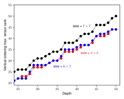
Figure 4: Treewidth for circuits from Ref. Boixo et al. (2016) with $6\times 6$, $7\times 6$, and $7\times 7$ qubits as a function of the circuit depth using a vertical elimination ordering, one circuit instance in each case. There are small variations between instances of the same size.

Figure 4 shows the size of the maximun tensor rank as a function of the circuit depth for an instance of each size $6\times 6$, $6\times 7$, and $7\times 7$ using a vertical elimination ordering. More exactly, we plot the size of the tensor minus 1, to make it directly comparable to the standard definition of treewidth used in Fig. 5. There are small variations between instances of the same size, which explains that in this particular case the instance of size $6\times 7$ has a larger tensor size for some depths in this ordering than the instance of size $7\times 7$.

IV.2 Numerical estimation of the treewidth for some quantum circuits

The size of the factors obtained by variable elimination from a given ordering can be analyzed graphically. We start with the undirected graph corresponding to the original expression, where each variable corresponds to a vertex. To simulate the elimination of a variable, we add an edge between all vertices connected to the vertex (variable) being eliminated. The cliques obtained in this process correspond to factors obtained through variable elimination. The size of the largest clique is called the induced width. Note that different orderings in the vertex elimination process, which correspond to different orderings of variable elimination, can result in different cliques. The treewidth is defined as the minimum width over all variable orderings. Determining the treewidth is in general NP-complete, but heuristic algorithms, such as QuickBB Gogate and Dechter (2004), can be used to obtain an approximation.

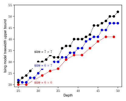
Figure 5: Numerical upper bound for the treewidth of the undirected graphical model corresponding to circuits from Ref. Boixo et al. (2016) with $6\times 6$, $6\times 7$, and $7\times 7$ qubits as a function of the circuit depth.

For a circuit in a 2D lattice of qubits with two-qubit gates restricted to nearest neighbors, as in Ref. Boixo et al. (2016), the treewidth of the corresponding undirected graphical model is proportional to $\min(O(d\ell),O(n))$, where $\ell$ is the minimum lateral dimension. Figure 5 shows numerical upper bounds for the treewidth as a function of depth (see also Ref. Boixo et al. (2016)). The upper bounds were obtained by running the QuickBB algorithm Gogate and Dechter (2004). This algorithm also returns the corresponding variable elimination order, which was used in Fig. 2 and also to calculate the probabilities plotted in Fig. 3.

V Conclusion

We generalize the simulation of a quantum circuit by mapping it onto an undirected graphical model, which we compute using the variable elimination algorithm, developed in the context of exact inference Dechter (1998); Bishop and ligne) (2006); Murphy (2012). This is particularly convenient for circuits of low depth Markov and Shi (2008); Boixo et al. (2016); Aaronson and Chen (2016), and with predominantly diagonal two-qubit gates. We are able to sample the output distribution of quantum circuits in a single workstation for cases that previously required a supercomputer. We also show how to perform cross entropy benchmarking and how to estimate the value of an observable. The computation of many amplitudes is embarrassingly parallelizable across machines. The cost of this algorithm is exponential in $\min(O(d\ell),O(n))$ for depth $d$, minimun lateral dimension $\ell$ and total number of qubits $n$. More optimally, the cost is exponential in the treewidth of the graph, as estimated in Ref. Boixo et al. (2016). Follow up work will study potential improvements to this algorithm, such as implementation in a supercomputer and code optimization, and possible space-time tradeoffs Aaronson and Chen (2016).

Appendix A Pseudocode

In this section we give pseudocode for the quantum circuit simulation algorithm presented in the main text Murphy (2012). As seen in Eq. (6), an output amplitude of a quantum circuit is expressed as a sum of products of factors. Each factor is a complex valued function or tensor defined in one or two Boolean variables or indexes. The variable elimination algorithm performs the sum of Eq. (6) eliminating one variable at a time, see Eq. (18). Larger tensors are created in the process. In what follows we assume that all Boolean variables have been given an appropriate order for variable elimination, see Secs. IV.1 and IV.2.

The basic objects of the computation are tensors. Tensors are complex functions defined on Boolean variables. Variables are associated with vertices in the undirected graphical model as explained in Sec. III.2. Tensors implement two operations. One is a multiplication across tensors, tensor1 * tensor2, implemented with broadcasting semantics, as in the NumPy python library. This means that the product of tensors is done elementwise. If an index or variable in tensor_a is missing in tensor_b then, in effect, this index is added to tensor_b with dimension 1 (the value of tensor_b is determined by the pre-existing indexes). The other operation, tensor.reduce_sum(), computes the sum of elements across the first dimension of the tensor. For simplicity, we assume that the indexes of all tensors are initially ordered from low to high. This will also be an invariant of the algorithm.

The bucket elimination algorithm Dechter (1998); Kask et al. (2001) keeps track of the order of the operations involved. More explicitly, we use the bucket elimination algorithm to build a computational graph that will be processed by TensorFlow or Dask. A bucket is a list of tensors. The ordered list buckets has one bucket per variable. In this way each bucket is associated to a variable. An invariant of the algorithm is that each tensor in a bucket acts upon the variable associated with the bucket, and all other variables have higher order.

First we initialize each bucket with the tensors in Eq. (6), corresponding to the gates, initialization and measurement of a circuit output amplitude:

⬇

for tensor in initial_factors:

buckets[tensor.indexes[0]].append(tensor)

Note that this obeys the invariant given above, because of the assumption that the variables or indexes in each tensor are ordered from low to high.

Each bucket in the buckets list is processed in order. Processing a bucket implements the elimination of the variable associated with that bucket, as in Eq. (18). As noted above, we assume that variables have initially been ordered with the chosen variable elimination order. Processing the buckets list one by one then implements the correct order. Processing a bucket can return a tensor without indexes, corresponding to a scalar, when all tensors in the bucket had only one variable (this has to be the variable associated with the bucket). Typically this only happens in the last bucket, and this scalar corresponds to the amplitude that we want to calculate. In some cases, for circuits of very small depth, the circuit can be decomposed into disjoint tensors, and the corresponding scalars are multiplied together.

⬇

result = None

for bucket in buckets:

if not empty(bucket):

tensor = bucket.process_bucket()

if rank(tensor) > 0:

first_index = tensor.indexes[0]

to_bucket = buckets[first_index]

to_bucket.append(tensor)

else:

if result:

result *= tensor

else:

result = tensor

return result

The processing of a bucket consists on two steps: first all tensors in the bucket are broadcasted together, and then the first variable is summed over, as in Eq. (18). By the invariants of the algorithm, the variable summed over is the one associated to the bucket.

⬇

def process_bucket(bucket):

result = bucket.tensors[0]

for tensor in bucket.tensors[1:]:

result *= tensor

# reduce

return result.reduce_sum()

Appendix B Cross entropy benchmarking

We now review cross entropy benchmarking, a technique to estimate the fidelity of an experimental quantum circuit implementation using the exact probabilities amplitudes calculated by a quantum circuit simulation algorithm Boixo et al. (2016); Neill et al. (2017).

The cross-entropy between a probability distribution $p_{A}$ and the ideal output probability $p_{\mathcal{U}}$ is defined as $S(p_{A},p_{\mathcal{U}})=-\sum_{x}p_{A}(x)\log p_{\mathcal{U}}(x)$. As explained in Ref. Boixo et al. (2016), the cross-entropy with an uncorrelated distribution $p_{\rm unc}$ averaged over quantum circuits is almost constant, ${\rm H}_{0}={\mathbb{E}}_{\mathcal{U}}[S(p_{\rm unc},p_{U})]$. In the following we make the averaging over circuits ${\mathcal{U}}$ implicitly.

We write the output of an experimental quantum circuit implementation with fidelity $\alpha$ as

$$\rho=\alpha\,{\mathcal{U}}\mathinner{|{0}\rangle}\!\mathinner{\langle{0}|}{\mathcal{U}}^{\dagger}+(1-\alpha)\sigma_{\mathcal{U}}\;.$$ (19)

The state ${\mathcal{U}}\mathinner{|{0}\rangle}$ corresponds to the ideal output of circuit ${\mathcal{U}}$, without any errors, while $\sigma_{\mathcal{U}}$ represents the output of the implementation of ${\mathcal{U}}$ after any experimental errors. The experimental output probability for a bit-string $x$ is $p_{\rm exp}(x)=\mathinner{\langle{x}|}\rho\mathinner{|{x}\rangle}=\alpha\,p_{\mathcal{U}}(x)+(1-\alpha)\mathinner{\langle{x}|}\sigma_{\mathcal{U}}\mathinner{|{x}\rangle}$. From the arguments presented in Ref. Boixo et al. (2016), almost any error in a random universal circuit of sufficient depth results in an output probability which is uncorrelated with the ideal probability distribution, and therefore we assume that $\mathinner{\langle{x}|}\sigma_{\mathcal{U}}\mathinner{|{x}\rangle}$ is uncorrelated with $p_{\mathcal{U}}(x)$. We have

$${\rm H}_{0}-S(p_{\rm exp},p_{\mathcal{U}})$$ (20)

$$={\rm H}_{0}+\sum_{j}\big{(}\alpha p_{\mathcal{U}}(x_{j})$$

$$\quad\quad+(1-\alpha)\mathinner{\langle{x_{j}}|}\sigma_{\mathcal{U}}\mathinner{|{x_{j}}\rangle}\big{)}\log p_{\mathcal{U}}(x_{j})$$ (21)

$$={\rm H}_{0}-\alpha{\rm H}(p_{\mathcal{U}})-(1-\alpha){\rm H}_{0}$$ (22)

$$=\alpha({\rm H}_{0}-{\rm H}(p_{\mathcal{U}}))\;.$$ (23)

Therefore

$$\alpha={{\rm H}_{0}-S(p_{\rm exp},p_{\mathcal{U}})\over{\rm H}_{0}-{\rm H}(p_{\mathcal{U}})}$$ (24)

is an estimate of the experimental fidelity. Note that ${\rm H}_{0}$ and ${\rm H}(p_{\mathcal{U}})$ can be calculated numerically, see Sec. II and App. C. Furthermore, for universal random circuits in the Porter-Thomas regime we have ${\rm H}_{0}=\log(2^{n})+\gamma$ and ${\rm H}(p_{\mathcal{U}})=\log(2^{n})-1+\gamma$, where $\gamma$ is Euler’s constant Boixo et al. (2016).

In order to estimate the fidelity $\alpha$ of an experimental implementation, we take a large sample $S_{\rm exp}=\{x_{1}^{\rm exp},\ldots,x_{m}^{\rm exp}\}$ of bit-strings $x$ in the computational basis ($m\sim 10^{3}-10^{6}$). From the central limit theory we have (see App. C)

$$-\frac{1}{m}\sum_{j=1}^{m}\log p_{U}(x_{j}^{\rm exp})$$ (25)

$$=-\sum_{x}p_{\rm exp}(x)\log p_{\mathcal{U}}(x)+O(1/\sqrt{m})$$ (26)

$$=S(p_{\rm exp},p_{\mathcal{U}})+O(1/\sqrt{m})\;.$$ (27)

In conclusion, using the algorithm presented in the main text to calculate the $m$ ideal output probabilities $\{p_{\mathcal{U}}(x^{\rm exp})\}$, we can use Eqs. (25) and (24) to obtain an estimate of $\alpha$.

Appendix C Random circuit sampling with a set of probabilities

Assume that we are asked to perform the following computational task: sample a set of bit-strings $S$ from the output distribution $\{p_{\mathcal{U}}(x)\}$ defined by a quantum circuit ${\mathcal{U}}$. In order to simulate sampling from the output distribution $\{p_{\mathcal{U}}(x)\}$ using the algorithm above, we start with a set $T=\{x_{j}\}$ of bit-strings selected uniformly at random. We denote the size of $T$ as $t$. We then calculate the probabilities $\{p_{\mathcal{U}}(x_{j})\}$ corresponding to the circuit ${\mathcal{U}}$ and sample from the set $T$ according to the normalized probabilities $\tilde{p}_{\mathcal{U}}(x_{j})$

$$\tilde{p}_{\mathcal{U}}(x_{j}) ={p_{\mathcal{U}}(x_{j})\over\sum_{j\in T}p_{\mathcal{U}}(x_{j})}=\frac{2^{n}}{t}\left(1+O\left({1\over\sqrt{t}}\right)\right)p_{\mathcal{U}}(x_{j})\;.$$ (28)

Note that by standard arguments in Monte Carlo integration, and given that the variance of the relevant distribution for random circuits is a constant $\sim 1$ Boixo et al. (2016), we can approximate any function defined over the output probabilities of the circuit using the set $T$ up to an error $\sim 1/\sqrt{t}$.

In particular, if we take a sample $S$ of size $m$ from $T$ according to the probabilities $\{\tilde{p}_{\mathcal{U}}(x_{j})\}$ we would get an estimate of the cross entropy of this sample

$$-\frac{1}{m}\sum_{j\in S}\log p_{\mathcal{U}}(x_{j})$$

$$=-\sum_{j\in T}\tilde{p}_{\mathcal{U}}(x_{j})\log p_{\mathcal{U}}(x_{j})+O\left(\frac{1}{\sqrt{m}}\right)$$

$$=-\frac{2^{n}}{t}\left(1+O\left({1\over\sqrt{t}}\right)\right)\sum_{j\in T}p_{\mathcal{U}}(x_{j})\log p_{\mathcal{U}}(x_{j})+O\left(\frac{1}{\sqrt{m}}\right)$$

$$=H({\mathcal{U}})+O\left({1\over\sqrt{t}}\right)H({\mathcal{U}})+O\left(\frac{1}{\sqrt{m}}\right)\;,$$ (29)

where $H({\mathcal{U}})$ is the entropy of the output distribution defined by circuit ${\mathcal{U}}$. That is, according to the cross entropy difference (see Eq. (24) and Ref. Boixo et al. (2016)), our simulation is sampling from the ideal circuit with high fidelity, because we obtain the correct entropy.

A more detailed calculation shows that the cross entropy obtained this way is distributed according to

$$H({\mathcal{U}})-\xi\sqrt{2/t}\,H({\mathcal{U}})+\zeta\sqrt{(\pi^{2}/6-1)/m}\\ +\xi\zeta\frac{n^{2}}{\sqrt{2tm(\pi^{2}/6-1)}}\;,$$ (30)

where $\xi$ and $\zeta$ and independent random variables that obey the normal distribution $N(0,1)$.

Note that the error or order $1/\sqrt{m}$ comes from simulating a sample of size $S$ out of the set $T$ of output probabilities that have been calculated. This error is avoided if we estimate an observable directly from $T$.

Appendix D Simulation example

In this appendix we consider the specific example of the quantum circuit

$$\begin{aligned} \lx@xy@svg{\hbox{\raise 0.0pt\hbox{\kern 0.0pt\hbox{\ignorespaces\ignorespaces\ignorespaces\hbox{\vtop{\kern 0.0pt\offinterlineskip\halign{\entry@#!@&&\entry@@#!@\cr&&&&\\&&&&\\}}}\ignorespaces{\hbox{\kern 0.0pt\raise 0.0pt\hbox{\hbox{\kern-18.88887pt\raise-2.5pt\hbox{$\textstyle{\mathinner{|{0}\rangle}}$}}}}}{\hbox{\kern 2.4375pt\raise 0.0pt\hbox{\hbox{\kern 3.00003pt\raise-3.41666pt\hbox{$\textstyle{H}$}}}}}\ignorespaces\ignorespaces\ignorespaces\ignorespaces{\hbox{\lx@xy@droprule}}\ignorespaces\ignorespaces\ignorespaces{\hbox{\lx@xy@droprule}}\ignorespaces\ignorespaces\ignorespaces{\hbox{\lx@xy@droprule}}\ignorespaces\ignorespaces\ignorespaces{\hbox{\lx@xy@droprule}}\ignorespaces\ignorespaces\ignorespaces\ignorespaces{}{\hbox{\lx@xy@droprule}}\ignorespaces{}{\hbox{\lx@xy@droprule}}{\hbox{\lx@xy@droprule}}{\hbox{\kern 27.73682pt\raise 0.0pt\hbox{\hbox{\kern-1.27777pt\raise-2.47217pt\hbox{$\textstyle{\bullet}$}}}}}\ignorespaces\ignorespaces\ignorespaces\ignorespaces{}{\hbox{\lx@xy@droprule}}\ignorespaces{}{\hbox{\lx@xy@droprule}}{\hbox{\lx@xy@droprule}}\ignorespaces\ignorespaces\ignorespaces\ignorespaces{}{\hbox{\lx@xy@droprule}}\ignorespaces{}{\hbox{\lx@xy@droprule}}{\hbox{\lx@xy@droprule}}{\hbox{\kern 40.35556pt\raise 0.0pt\hbox{\hbox{\kern 3.00003pt\raise-3.41666pt\hbox{$\textstyle{H}$}}}}}\ignorespaces\ignorespaces\ignorespaces\ignorespaces{\hbox{\lx@xy@droprule}}\ignorespaces\ignorespaces\ignorespaces{\hbox{\lx@xy@droprule}}\ignorespaces\ignorespaces\ignorespaces{\hbox{\lx@xy@droprule}}\ignorespaces\ignorespaces\ignorespaces{\hbox{\lx@xy@droprule}}\ignorespaces\ignorespaces\ignorespaces\ignorespaces{}{\hbox{\lx@xy@droprule}}\ignorespaces{}{\hbox{\lx@xy@droprule}}{\hbox{\lx@xy@droprule}}{\hbox{\kern 48.91808pt\raise 0.0pt\hbox{\hbox{\kern-12.99998pt\raise 0.0pt\hbox{$\textstyle{\lx@xy@svgnested{\hbox{\raise 0.0pt\hbox{\kern 22.0pt\hbox{\ignorespaces\ignorespaces\ignorespaces\ignorespaces\hbox{\ignorespaces\ignorespaces\ignorespaces\ignorespaces\ignorespaces\ignorespaces{\ignorespaces}\ignorespaces\ignorespaces\ignorespaces\ignorespaces\ignorespaces\ignorespaces\ignorespaces{\ignorespaces\ignorespaces}\ignorespaces\ignorespaces\ignorespaces{}{}\ignorespaces\ignorespaces\ignorespaces{}\ignorespaces\hbox{\hbox{\kern 0.0pt\raise 0.0pt\hbox{{{}{}{{{}{}{}{}{{{{{}}}{{{}}{{{}}{{{}}{{{}}{{{}}{{{}}{{{}}{{{}}}{{}}{{}}{{{}}}{{}}{{}}{{{}}}{{}}{{}}{{{}}}{{}}{{}}{{{}}}{{}}{{}}{{{}}}{{}}{{}}{{{}}}}}}}}}}}}}}}{{}{}{}{}\lx@xy@spline@}{}}}}}\ignorespaces\ignorespaces\ignorespaces{\hbox{\lx@xy@drawline@}}\ignorespaces{}\ignorespaces{}}}}}}$}}}}}\ignorespaces\ignorespaces\ignorespaces\ignorespaces{\hbox{\lx@xy@droprule}}\ignorespaces\ignorespaces\ignorespaces{\hbox{\lx@xy@droprule}}\ignorespaces\ignorespaces\ignorespaces{\hbox{\lx@xy@droprule}}\ignorespaces\ignorespaces\ignorespaces{\hbox{\lx@xy@droprule}}\ignorespaces\ignorespaces\ignorespaces\ignorespaces{}{\hbox{\lx@xy@droprule}}\ignorespaces{}{\hbox{\lx@xy@droprule}}{\hbox{\kern 0.0pt\raise-25.83327pt\hbox{\hbox{\kern-18.88887pt\raise-2.5pt\hbox{$\textstyle{\mathinner{|{0}\rangle}}$}}}}}{\hbox{\kern 2.4375pt\raise-25.83327pt\hbox{\hbox{\kern 3.00003pt\raise-3.41666pt\hbox{$\textstyle{H}$}}}}}\ignorespaces\ignorespaces\ignorespaces\ignorespaces{\hbox{\lx@xy@droprule}}\ignorespaces\ignorespaces\ignorespaces{\hbox{\lx@xy@droprule}}\ignorespaces\ignorespaces\ignorespaces{\hbox{\lx@xy@droprule}}\ignorespaces\ignorespaces\ignorespaces{\hbox{\lx@xy@droprule}}\ignorespaces\ignorespaces\ignorespaces\ignorespaces{}{\hbox{\lx@xy@droprule}}\ignorespaces{}{\hbox{\lx@xy@droprule}}{\hbox{\lx@xy@droprule}}{\hbox{\kern 27.73682pt\raise-25.83327pt\hbox{\hbox{\kern-1.27777pt\raise-2.47217pt\hbox{$\textstyle{\bullet}$}}}}}\ignorespaces\ignorespaces\ignorespaces\ignorespaces{}{\hbox{\lx@xy@droprule}}\ignorespaces{}{\hbox{\lx@xy@droprule}}{\hbox{\lx@xy@droprule}}\ignorespaces\ignorespaces\ignorespaces\ignorespaces{}{\hbox{\lx@xy@droprule}}\ignorespaces{}{\hbox{\lx@xy@droprule}}{\hbox{\lx@xy@droprule}}{\hbox{\kern 40.35556pt\raise-25.83327pt\hbox{\hbox{\kern 3.00003pt\raise-3.41666pt\hbox{$\textstyle{H}$}}}}}\ignorespaces\ignorespaces\ignorespaces\ignorespaces{\hbox{\lx@xy@droprule}}\ignorespaces\ignorespaces\ignorespaces{\hbox{\lx@xy@droprule}}\ignorespaces\ignorespaces\ignorespaces{\hbox{\lx@xy@droprule}}\ignorespaces\ignorespaces\ignorespaces{\hbox{\lx@xy@droprule}}\ignorespaces\ignorespaces\ignorespaces\ignorespaces{}{\hbox{\lx@xy@droprule}}\ignorespaces{}{\hbox{\lx@xy@droprule}}{\hbox{\lx@xy@droprule}}{\hbox{\kern 48.91808pt\raise-25.83327pt\hbox{\hbox{\kern-12.99998pt\raise 0.0pt\hbox{$\textstyle{\lx@xy@svgnested{\hbox{\raise 0.0pt\hbox{\kern 22.0pt\hbox{\ignorespaces\ignorespaces\ignorespaces\ignorespaces\hbox{\ignorespaces\ignorespaces\ignorespaces\ignorespaces\ignorespaces\ignorespaces{\ignorespaces}\ignorespaces\ignorespaces\ignorespaces\ignorespaces\ignorespaces\ignorespaces\ignorespaces{\ignorespaces\ignorespaces}\ignorespaces\ignorespaces\ignorespaces{}{}\ignorespaces\ignorespaces\ignorespaces{}\ignorespaces\hbox{\hbox{\kern 0.0pt\raise 0.0pt\hbox{{{}{}{{{}{}{}{}{{{{{}}}{{{}}{{{}}{{{}}{{{}}{{{}}{{{}}{{{}}{{{}}}{{}}{{}}{{{}}}{{}}{{}}{{{}}}{{}}{{}}{{{}}}{{}}{{}}{{{}}}{{}}{{}}{{{}}}{{}}{{}}{{{}}}}}}}}}}}}}}}{{}{}{}{}\lx@xy@spline@}{}}}}}\ignorespaces\ignorespaces\ignorespaces{\hbox{\lx@xy@drawline@}}\ignorespaces{}\ignorespaces{}}}}}}$}}}}}\ignorespaces\ignorespaces\ignorespaces\ignorespaces{\hbox{\lx@xy@droprule}}\ignorespaces\ignorespaces\ignorespaces{\hbox{\lx@xy@droprule}}\ignorespaces\ignorespaces\ignorespaces{\hbox{\lx@xy@droprule}}\ignorespaces\ignorespaces\ignorespaces{\hbox{\lx@xy@droprule}}\ignorespaces\ignorespaces\ignorespaces\ignorespaces{}{\hbox{\lx@xy@droprule}}\ignorespaces{}{\hbox{\lx@xy@droprule}}\ignorespaces}}}}\ignorespaces\end{aligned} \textstyle{\mathinner{|{0}\rangle}} \textstyle{H} \textstyle{\bullet} \textstyle{H} \textstyle{\mathinner{|{0}\rangle}} \textstyle{H} \textstyle{\bullet} \textstyle{H} \textstyle{\mathinner{|{0}\rangle}} \textstyle{H} \textstyle{\bullet} \textstyle{H} \textstyle{\mathinner{|{0}\rangle}} \textstyle{H} \textstyle{\bullet} \textstyle{H}$$ (31)

We calculate the output amplitude for input $\mathinner{|{00}\rangle}$ and output $\mathinner{|{00}\rangle}$. The corresponding graphical model is

$$\begin{aligned} \leavevmode\hbox to107.8pt{\vbox to65.12pt{\text{[drawing]}}}\;.\end{aligned} b_{0}^{0} b_{0}^{1} b_{0}^{2} b_{1}^{0} b_{1}^{1} b_{1}^{2} b_{0}^{0} b_{0}^{1} b_{0}^{2} b_{1}^{0} b_{1}^{1} b_{1}^{2}$$ (32)

Because the input and output is specified, we have $b_{0}^{0}$ $=$ $b_{0}^{2}$ $=$ $b_{1}^{0}$ $=$ $b_{1}^{2}$ $=$ 0. Then the graph can be simplified to

$$\begin{aligned} \leavevmode\hbox to22.44pt{\vbox to65.12pt{\text{[drawing]}}}\;.\end{aligned} b_{0}^{1} b_{1}^{1} b_{0}^{1} b_{1}^{1}$$ (33)

The treewidth of this graph is 2, because it is a clique with two vertices. In the next step we can eliminate the variables $b_{0}^{1}$ and $b_{1}^{1}$ in any order.

More explicitly, the amplitude $\mathinner{\langle{00}|}C\mathinner{|{00}\rangle}$, where $C$ is the circuit in Fig. (31), is

$$\mathinner{\langle{00}|}C\mathinner{|{00}\rangle}=\sum_{b_{0}^{1},b_{1}^{1}}\psi_{\rm H}(0,b_{0}^{1})\psi_{\rm CZ}(b_{0}^{1},b_{1}^{1})\psi_{\rm H}(b_{0}^{1},0)\\ \psi_{\rm H}(0,b_{1}^{1})\psi_{\rm H}(b_{1}^{1},0)\;.$$ (34)

The function $\psi_{\rm H}$ corresponds to a Hadamard gate and is given by the table

0	0	$1/\sqrt{2}$
0	1	$1/\sqrt{2}$
1	0	$1/\sqrt{2}$
1	1	$-1/\sqrt{2}$

The function $\psi_{\rm CZ}$ corresponds to a controlled-Z gate and is given by the table

0	0	$1$
0	1	$1$
1	0	$1$
1	1	$-1$

We can rewrite Eq. (34) as

$$\mathinner{\langle{00}|}C\mathinner{|{00}\rangle}=\sum_{b_{0}^{1},b_{1}^{1}}\tau_{1}(b_{0}^{1},b_{1}^{1})$$ (35)

where the table for the function $\tau_{1}$ is

0	0	$1/4$
0	1	$1/4$
1	0	$1/4$
1	1	$-1/4$

If we now sum over the variable $b_{1}^{1}$ we obtain

$$\mathinner{\langle{00}|}C\mathinner{|{00}\rangle}=\sum_{b_{0}^{1}}\tau_{2}(b_{0}^{1})$$ (36)

where the function $\tau_{2}$ is

0	$1/2$
1	0

Finally, summing $b_{0}^{1}$ we obtain

$$\mathinner{\langle{00}|}C\mathinner{|{00}\rangle}=1/2\;.$$ (37)

Appendix E Relation to tensor network contraction

Variable elimination on the undirected graph representing a quantum circuit is related to the simulation of a quantum circuit by contracting tensor networks Markov and Shi (2008). In a tensor network graphical representation, gates correspond to vertices (tensors) and qubits connecting gates (indexes in the tensors) are represented by edges. Therefore, a two-qubit gate is represented as a node with four edges, two for input and two for output. For instance, the tensor network corresponding to the example of Eq. (14) is

$$\leavevmode\hbox to123.64pt{\vbox to38.28pt{\text{[drawing]}}}\;.$$ (38)

The operation of contracting a network of tensors is analogous to the variable elimination in Sec. IV. The indexes in common are summed over or contracted, and the size of the resulting tensor in memory is exponential in the number of remaining indices. Graphically, the contraction of two tensors is represented by eliminating the edges (indexes) that the corresponding two vertices (tensors) have in common, and replacing both vertices with a single vertex with the remaining edges (indexes). As in variable elimination, the cost also depends in the order in which indexes are eliminated.

Reference Markov and Shi (2008) relates the minimum cost of the tensor contraction to the treewidth of the corresponding line graph. The line graph $G^{\prime}$ corresponding to the graph $G$ representing the tensor network is defined with a vertex for every edge in $G$. If two edges are incident in the same vertex (tensor) in $G$, then we add an edge in $G^{\prime}$ between the corresponding two vertices of $G^{\prime}$. In this way a two-qubit gate (a tensor with four indexes) results in a clique between four vertices in the line graph. For instance, the line graph corresponding to the tensor network in (38) is

$$\leavevmode\hbox to95.19pt{\vbox to38.28pt{\text{[drawing]}}}\;.$$ (39)

It follows that the line graph of the tensor network for a quantum circuit is analogous to the undirected graphical model detailed above. The main difference is that diagonal two-qubit (and single-qubit) gates are treated more efficiently in the undirected graphical model obtained directly from the quantum circuit factor representation. In the line graph obtained from a tensor network a diagonal gate results in a clique with four vertices, but in the original graphical model is represented only by an edge and does not introduce new vertices. This can be seen comparing the examples in Fig. 32, with treewidth 2, and (39), which has treewidth 4. Because the cost is exponential in the treewidth, this optimization results in a smaller exponent for the computation.

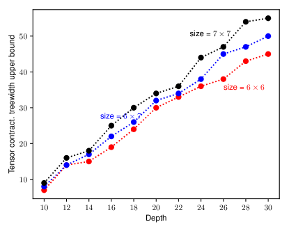
Figure 6: Numerical upper bound for the treewidth of the line graph which gives the tensor contraction complexity Markov and Shi (2008) of circuits from Ref. Boixo et al. (2016) with $6\times 6$, $6\times 7$, and $7\times 7$ qubits as a function of the circuit depth.

Figure 6 shows numerical upper bounds for the treewidth of the line graph as a function of depth for the circuits in Ref. Boixo et al. (2016). The upper bounds were also obtained by running the QuickBB algorithm Gogate and Dechter (2004). Now that the treewidth has been reduced by almost a factor of two in the undirected graphical model which is drawn directly from the quantum circuit, Fig. 5, instead of using the line graph of the tensor network, Fig. 6. This is due to the fact that in these circuits all two-qubit gates are controlled-Z gates.

Appendix F The partition function for random circuits

We review the direct mapping of random circuits to a partition function of an Ising model at imaginary temperature from Ref. Boixo et al. (2016). Previous algorithms for mapping universal quantum circuits to partition functions of complex Ising models use polynomial reductions to a universal gate set Lidar (2004); Geraci and Lidar (2010); De las Cuevas et al. (2011), which make them less efficient.

We encode each individual Feynman path by the set of $L$ binary variables or spins $s=\{s_{j}^{k}\}$ with $j\in[1\mathrel{{.}\,{.}}\nobreak n]$, $k\in[0\mathrel{{.}\,{.}}\nobreak d_{j}]$ and $s_{j}^{k}\in\{1,-1\}$. One can easily see from the explicit form of the non-diagonal gates in our example that the absolute values of the probability amplitudes associated with different paths are all the same and equal to $2^{-L/2}$. Using this fact we write the path integral (1) in the following form

$$\langle x|{\mathcal{U}}|0\ldots 0\rangle=2^{-L/2}\sum_{s}{\rm exp}\left(\frac{i\pi}{4}H_{s}(x)\right)\;.$$ (40)

Here ${\rm exp}(i\pi H_{s}(x)/4)$ is a phase factor associated with each path that depends explicitly on the end-point condition (2).

The value of the phase $\pi H_{s}/4$ is accumulated as a sum of discrete phase changes that are associated with individual gates. For the $k$-th non-diagonal gate applied to qubit $j$ we introduce the coefficient $\alpha_{j}^{k}$ such that $\alpha_{j}^{k}=1$ if the gate is ${\rm X}^{1/2}$ and $\alpha_{j}^{k}=0$ if the gate is ${\rm Y}^{1/2}$. Thus, the total phase change accumulated from the application of ${\rm X}^{1/2}$ and ${\rm Y}^{1/2}$ gates equals

$$\frac{i\pi}{4}H_{s}^{{\rm X}^{1/2}}(x) =\frac{i\pi}{2}\sum_{j=1}^{n}\sum_{k=0}^{d_{j}}\alpha_{j}^{k}\frac{1+s_{j}^{k-1}s_{j}^{k}}{2}\;,$$ (41)

$$\frac{i\pi}{4}H_{s}^{{\rm Y}^{1/2}}(x) =i\pi\sum_{j=1}^{n}\sum_{k=0}^{d_{j}}(1-\alpha_{j}^{k})\frac{1-s_{j}^{k-1}}{2}\frac{1+s_{j}^{k}}{2}\;\;.$$

As mentioned above, the dependence on $x$ arises due to the boundary condition (2). Note that we have omitted constant phase terms that do not depend on the path $s$.

We now describe the phase change from the action of gates ${\rm T}$ and ${\rm CZ}$. We introduce coefficients $d(j,t)$ equal to the number of non-diagonal gates applied to qubit $j$ over the first $t$ cycles (including the $0$-th cycle of Hadamard gates). We also introduce coefficients $\tau_{j}^{t}$ such that $\tau_{j}^{t}=1$ if a ${\rm T}$ gate is applied at cycle $t$ to qubit $j$ and $\tau_{j}^{t}=0$ otherwise. Then the total phase accumulated from the action of the ${\rm T}$ gates equals

$$\frac{i\pi}{4}H_{s}^{T}(x)=\frac{i\pi}{4}\sum_{j=1}^{n}\sum_{t=0}^{d}\tau_{j}^{t}\frac{1-s_{j}^{d(j,t)}}{2}\;.$$ (42)

For a given pair of qubits $(i,j)$, we introduce coefficients $z_{ij}^{t}$ such that $z_{ij}^{t}=1$ if a ${\rm CZ}$ gate is applied to the qubit pair during cycle $t$ and $z_{ij}^{t}=0$ otherwise. The total phase accumulated from the action of the ${\rm CZ}$ gates equals

$$\frac{i\pi}{4}H_{s}^{{\rm CZ}}(x)\\ =i\pi\sum_{i=1}^{n}\sum_{j=1}^{i-1}\sum_{t=0}^{d}z_{ij}^{t}\frac{1-s_{i}^{d(i,t)}}{2}\frac{1-s_{j}^{d(j,t)}}{2}.$$ (43)

One can see from comparing (40) with (41)-(43) that the wavefunction amplitudes $\langle x|U|0\ldots 0\rangle$ take the form of a partition function of a classical Ising model with energy $H_{s}$ for a state $s$ and purely imaginary inverse temperature $i\pi/4$. The total phase for each path takes 8 distinct values (mod 2$\pi$) equal to $[0,\pi/4\mathrel{{.}\,{.}}\nobreak 7\pi/4]$. The interaction graph of this Ising model is the undirected graphical model introduced in Sec. III.

Note that if a quantum circuit uses only Clifford gates (not ${\rm T}$ gates), the total phase for each spin configuration in the partition function (mod 2$\pi$) is restricted to $[0,\pi/2,\pi,3\pi/2]$. In these case, the corresponding partition function can be calculated efficiently in polynomial time Gottesman (1998); Fujii and Morimae (2017); Goldberg and Guo (2014).

References

• Boixo et al. (2016) S. Boixo, S. V. Isakov, V. N. Smelyanskiy, R. Babbush, N. Ding, Z. Jiang, J. M. Martinis,  and H. Neven, arXiv:1608.00263  (2016).
• Feynman (1982) R. P. Feynman, Int. J. Theor. Phys. 21, 467 (1982).
• Aspuru-Guzik et al. (2005) A. Aspuru-Guzik, A. D. Dutoi, P. J. Love,  and M. Head-Gordon, Science 309, 1704 (2005).
• Hastings et al. (2015) M. B. Hastings, D. Wecker, B. Bauer,  and M. Troyer, QIC 15, 1 (2015).
• Wecker et al. (2015) D. Wecker, M. B. Hastings, N. Wiebe, B. K. Clark, C. Nayak,  and M. Troyer, Phys. Rev. A 92, 062318 (2015).
• O’Malley et al. (2016) P. O’Malley, R. Babbush, I. Kivlichan, J. Romero, J. McClean, R. Barends, J. Kelly, P. Roushan, A. Tranter, N. Ding, et al., Phys. Rev. X 6, 031007 (2016).
• Reiher et al. (2017) M. Reiher, N. Wiebe, K. M. Svore, D. Wecker,  and M. Troyer, PNAS , 201619152 (2017).
• Babbush et al. (2017) R. Babbush, N. Wiebe, J. McClean, J. McClain, H. Neven,  and G. K. Chan, arXiv:1706.00023  (2017).
• Jiang et al. (2017) Z. Jiang, K. J. Sung, K. Kechedzhi, V. N. Smelyanskiy,  and S. Boixo, arXiv:1711.05395  (2017).
• Shor (1999) P. W. Shor, SIAM review 41, 303 (1999).
• Aaronson and Arkhipov (2011) S. Aaronson and A. Arkhipov, in STOC (ACM, 2011) pp. 333–342.
• Bremner et al. (2016a) M. J. Bremner, A. Montanaro,  and D. J. Shepherd, Phys. Rev. Lett. 117, 080501 (2016a).
• Bremner et al. (2016b) M. J. Bremner, A. Montanaro,  and D. J. Shepherd, arXiv:1610.01808  (2016b).
• Gao et al. (2017) X. Gao, S.-T. Wang,  and L.-M. Duan, Physical Review Letters 118, 040502 (2017).
• Hangleiter et al. (2017) D. Hangleiter, M. Kliesch, M. Schwarz,  and J. Eisert, QST 2, 015004 (2017).
• Kapourniotis and Datta (2017) T. Kapourniotis and A. Datta, arXiv:1703.09568  (2017).
• Neill et al. (2017) C. Neill, P. Roushan, K. Kechedzhi, S. Boixo, S. V. Isakov, V. Smelyanskiy, R. Barends, B. Burkett, Y. Chen, Z. Chen, B. Chiaro, A. Dunsworth, A. Fowler, B. Foxen, R. Graff, E. Jeffrey, J. Kelly, E. Lucero, A. Megrant, J. Mutus, M. Neeley, C. Quintana, D. Sank, A. Vainsencher, J. Wenner, T. C. White, H. Neven,  and J. M. Martinis, arXiv:1709.06678  (2017).
• Schack and Caves (1993) R. Schack and C. M. Caves, Phys. Rev. Lett. 71, 525 (1993).
• Scott et al. (2006) A. J. Scott, T. A. Brun, C. M. Caves,  and R. Schack, J. Phys. A: Math. Gen. 39, 13405 (2006).
• Barends et al. (2014) R. Barends, J. Kelly, A. Megrant, A. Veitia, D. Sank, E. Jeffrey, T. C. White, J. Mutus, A. G. Fowler, B. Campbell,  and others, Nature 508, 500 (2014).
• Fowler et al. (2012) A. G. Fowler, M. Mariantoni, J. M. Martinis,  and A. N. Cleland, Phys. Rev. A 86, 032324 (2012).
• De Raedt et al. (2007) K. De Raedt, K. Michielsen, H. De Raedt, B. Trieu, G. Arnold, M. Richter, T. Lippert, H. Watanabe,  and N. Ito, Computer Physics Communications 176, 121 (2007).
• Zulehner and Wille (2017) A. Zulehner and R. Wille, arXiv preprint arXiv:1707.00865  (2017).
• Häner and Steiger (2017) T. Häner and D. S. Steiger, arXiv:1704.01127  (2017).
• Pednault et al. (2017) E. Pednault, J. A. Gunnels, G. Nannicini, L. Horesh, T. Magerlein, E. Solomonik,  and R. Wisnieff, arXiv:1710.05867  (2017).
• Viamontes et al. (2009) G. F. Viamontes, I. L. Markov,  and J. P. Hayes, Quantum circuit simulation (Springer Science & Business Media, 2009).
• Dechter (1998) R. Dechter, in Learning in graphical models (Springer, 1998) pp. 75–104.
• Murphy (2012) K. P. Murphy, Machine learning: a probabilistic perspective, Adaptive computation and machine learning series (MIT Press, Cambridge, MA, 2012).
• Bernstein and Vazirani (1997) E. Bernstein and U. Vazirani, SIAMCOMP 26, 1411 (1997).
• Markov and Shi (2008) I. L. Markov and Y. Shi, SICOMP 38, 963 (2008).
• Aaronson and Chen (2016) S. Aaronson and L. Chen, arXiv:1612.05903  (2016).
• Martinis and Geller (2014) J. M. Martinis and M. R. Geller, Physical Review A 90 (2014), 10.1103/PhysRevA.90.022307.
• Barends et al. (2015) R. Barends, L. Lamata, J. Kelly, L. García-Álvarez, A. G. Fowler, A. Megrant, E. Jeffrey, T. C. White, D. Sank, J. Y. Mutus, B. Campbell, Y. Chen, Z. Chen, B. Chiaro, A. Dunsworth, I.-C. Hoi, C. Neill, P. J. J. O’Malley, C. Quintana, P. Roushan, A. Vainsencher, J. Wenner, E. Solano,  and J. M. Martinis, Nat. Comm. 6, 7654 (2015).
• Kelly et al. (2015) J. Kelly, R. Barends, A. G. Fowler, A. Megrant, E. Jeffrey, T. C. White, D. Sank, J. Y. Mutus, B. Campbell, Y. Chen,  and others, Nature 519, 66 (2015).
• Barends et al. (2016) R. Barends, A. Shabani, L. Lamata, J. Kelly, A. Mezzacapo, U. Las Heras, R. Babbush, A. Fowler, B. Campbell, Y. Chen, et al., Nature 534, 222 (2016).
• Abadi et al. (2016) M. Abadi, P. Barham, J. Chen, Z. Chen, A. Davis, J. Dean, M. Devin, S. Ghemawat, G. Irving, M. Isard, et al., in OSDI, Vol. 16 (2016) pp. 265–283.
• Gogate and Dechter (2004) V. Gogate and R. Dechter, in Proc CUAI (2004) pp. 201–208.
• (38) “Dask,” https://dask.pydata.org/en/latest/, accessed: 12-13-2017.
• Bishop and ligne) (2006) C. Bishop and S. S. e. ligne), Pattern recognition and machine learning, Vol. 4 (Springer New York, 2006).
• Boixo et al. (2014) S. Boixo, T. F. Rønnow, S. V. Isakov, Z. Wang, D. Wecker, D. A. Lidar, J. M. Martinis,  and M. Troyer, Nature Physics 10, 218 (2014).
• Kask et al. (2001) K. Kask, R. Dechter, J. Larrosa,  and F. Cozman, Artif. Intel 125, 131 (2001).
• Pearl (1982) J. Pearl, Reverend Bayes on inference engines: A distributed hierarchical approach (UCLA, 1982).
• Bethe (1935) H. A. Bethe, Proceedings of the Royal Society of London. Series A, Mathematical and Physical Sciences 150, 552 (1935).
• Mézard et al. (1987) M. Mézard, G. Parisi,  and M. Virasoro, Spin glass theory and beyond: An Introduction to the Replica Method and Its Applications, Vol. 9 (World Scientific Publishing Co Inc, 1987).
• Lidar (2004) D. A. Lidar, New J. Phys 6, 167 (2004).
• Geraci and Lidar (2010) J. Geraci and D. A. Lidar, New J. Phys 12, 075026 (2010).
• De las Cuevas et al. (2011) G. De las Cuevas, M. Van den Nest, M. Martin-Delgado, et al., New J. Phys. 13, 093021 (2011).
• Gottesman (1998) D. Gottesman, arXiv:quant-ph/9807006  (1998).
• Fujii and Morimae (2017) K. Fujii and T. Morimae, New J. Phys. 19, 033003 (2017).
• Goldberg and Guo (2014) L. A. Goldberg and H. Guo, arXiv:1409.5627  (2014).