One-Pass Graphic Approximation of Integer Sequences

Abstract

A variety of network modeling problems begin by generating a degree sequence drawn from a given probability distribution. If the randomly generated sequence is not graphic, we give a new approach for generating a graphic approximation of the sequence. This approximation scheme is fast, requiring only one pass through the sequence, and produces small probability distribution distances for large sequences.

1 Introduction

Model creation of real-world complex networks, such as social and biological interactions, remains an important area of research. The modeling and simulation of these systems often requires developing realistic graph models for the underlying networks embedded in these systems. A common first step in the creation of these graph models is to construct a graph with a given degree sequence. If we can construct a graph from an integer sequence, we say that the sequence is graphic.

One problem from the random modeling of graphs is selecting a graphic degree sequence from some given probability distribution. More specifically, how do we deal with a randomly drawn integer sequence that is not graphic? There have been two approaches to this problem. The first is to simply discard the sequence and repeatedly select a new sequence until a graphic sequence is found. This is the approach used by the NetworkX [1] graph library. A disadvantage to this approach is that for some probability distributions, the chance of selecting a graphic sequence is small. Thus the NetworkX library places an upper limit on the number of attempts to generate a graphic sequence before abandoning the task. This is potentially a computationally expensive task for very large sequences selected from a sequence with a small probability of being graphic.

In response to this difficulty, a second approach, suggested by Mihail and Vishoi [2], is to find the closest graphic sequence to the original non-graphic degree sequence using a given distance measure. Using a distance measure that they called the discrepancy, Mihail and Vishoi provided a polynomial-time algorithm for finding these graphic approximations by reducing this problem to maximum cardinality matching; unfortunately, their algorithm is not practical for many cases. They posed the question whether a practical algorithm for determining nearest graphical sequence under the discrepancy measure could be found. This question was answered by Hell and Kirkpatrick [3] who introduced two algorithms for computing a minimal discrepancy graphic sequence in lower polynomial time.

When Mihail and Vishoi considered this problem, they posed a couple of natural questions. The first is ”What is a natural notion of distance between two degree sequences?”, and the second is ”Are there efficient algorithms to approximate a non-graphic sequence with a graphic sequence whose distance is small?” We examine both of these questions and make a new contribution to the problem by introducing a new approach that requires only one pass through the sequence in order to give a graphic approximation. Further, we suggest that that minimizing distances between probability distributions, specifically the total variation distance, is a more appropriate approach to this problem. Finally, we show that under the total variation distance, the quality of the result from our approximation algorithm for many sequences improves as the size of the sequences increases.

2 Basic Results

Before introducing the algorithm, we need some preliminary definitions and results. A degree sequence $\alpha=\left(\alpha_{1},\alpha_{2},...,\alpha_{n}\right)$ is a set of non-negative integers such that $\alpha_{1}\geq\alpha_{2}\geq...\geq\alpha_{n}\geq 0$. As a notational convenience, if a value $a$ is represented $r$ times in a sequence we represent that subsequence as $a^{r}$, i.e.,

$$\left(\underbrace{a,...,a}_{r}\right)=\left(a^{r}\right).$$ (1)

If there exists a graph $G$ whose node degrees match the sequence $\alpha$, then $\alpha$ is said to be graphic; else, the sequence is called non-graphic.

If a sequence $\alpha$ has an even sum $s$ where $s\leq|\alpha|(|\alpha|-1)$, then we say that the sequence is potentially graphic. It is straightforward to see that any sequence that violates this condition is not graphic. Conversely, if this condition is met, then there exists some sequence having length $|\alpha|$ and sum $s$ that is graphic (this follows from Chen [4], Lemma 1). The minimal requirement for graphic approximation of a non-graphic sequence is that original sequence must be potentially graphic.

A tool we use to work with degree sequences is the partial ordering called majorization. A degree sequence $\alpha$ majorizes (or dominates) the integer sequence $\beta$, denoted by $\alpha\succcurlyeq\beta$, if for all $k$ from $1$ to $n$

$$\sum_{i=1}^{k}\alpha_{i}\geq\sum_{i=1}^{k}\beta_{i},$$ (2)

and if the sums of the two sequences are equal. If $\alpha\succcurlyeq\beta$ and there exists an index $k$ where $\sum_{i=1}^{k}\alpha_{i}>\sum_{i=1}^{k}\beta_{i}$, then we say that $\alpha$ strictly majorizes $\beta$, denoted as $\alpha\succ\beta$.

Over the set of integer partitions $\mathcal{L}_{p}$ for some positive integer $p$, majorization forms the lattice $(\mathcal{L}_{p},\succcurlyeq)$ [5] where the meet operator is defined as follows:

$$\begin{split}(\alpha\wedge\beta)_{k}&=\min\{\sum_{i=1}^{k}\alpha_{i},\sum_{i=1}^{k}\beta_{i}\}-\sum_{i=1}^{k-1}(\alpha\wedge\beta)_{i}\\ &=\min\{\sum_{i=1}^{k}\alpha_{i},\sum_{i=1}^{k}\beta_{i}\}-\min\{\sum_{i=1}^{k-1}\alpha_{i},\sum_{i=1}^{k-1}\beta_{i}\},\end{split}$$ (3)

For our purposes, the usefulness of comparing degree sequences using majorization stems from the following result which shows that every sequence that is majorized by a graphical sequence must also be graphical.

Theorem 1 (Ruch and Gutman [6], Theorem 1).

If the degree sequence $\alpha$ is graphic and $\alpha\succcurlyeq\beta$, then $\beta$ is graphic.

This result establishes the location of the graphic sequences in the lattice $(\mathcal{L}_{p},\succcurlyeq)$. If the integer $p$ is even, then there will be a small number of elements at the bottom of the partition lattice $\mathcal{L}_{p}$ that are graphic, while the remaining majority of the partitions will be non-graphic [7]. It also shows that the graphic sequences form a semi-lattice in $\mathcal{L}_{p}$.

A degree sequence which has precisely one labeled realization is called a threshold sequence and the resulting realization is called a threshold graph [8]. The following theorem shows that the threshold sequences sit at the top of the semi-lattice of graphic sequences.

Theorem 2 ([8], Theorem 3.2.2).

A graphic degree sequence $\alpha$ is threshold if and only if there does not exist a graphic sequence $\beta$ such that $\beta\succ\alpha$.

This next theorem provides a decomposition result that we can use to recognize threshold graphs (and, by extension, threshold sequences).

Theorem 3 ([8], Theorem 1.2.4).

A graph $G$ is threshold if and only if it can be constructed from a one-vertex by repeatedly adding either an isolated or dominating vertex.

3 A One-Pass Approximation Scheme

Our approximation scheme for the sequence $\alpha$ first involves creating a graphic sequence $T$ with the same length and sum as $\alpha$ and that has several desirable features. This sequence $T$ is defined as follows:

For the value $m=\min\{k|s\leq k\cdot(k-1)\}$,

$$T(n,s)=\begin{cases}\left(0^{n}\right)&\text{if $s=0$,}\\ \left(\gamma_{1},...,\gamma_{m},0^{n-m}\right)\text{ where $\gamma=T(m,s)$}&\text{if $n>m$,}\\ \left(n-1,\gamma_{1}+1,...,\gamma_{n-1}+1\right)\text{ where $\gamma=T(n-1,s-2\cdot(n-1))$}&\text{if $n\leq m$.}\\ \end{cases}$$

By comparing the definition of $T$ with Theorem 3, we see that $T(n,s)$ defines graphic threshold sequence. Thus, $T(n,s)$ is a maximal graphic sequence in the majorization lattice (Theorem 2). At the same time, from the definition, this sequence contains the minimum possible number of non-zero elements for a graphic sequence.

Additionally, an advantage in using the sequence $T$ is that we do not have to store or pre-compute this sequence. We can quickly compute any index of $T(n,s)$ in constant time as shown by the following result.

Theorem 4.

The sequence $T(n,s)=\left((p+1)^{q},p^{p+1-q},q,0^{n-p+2}\right)$ where

$$p=\left\lfloor\frac{\sqrt{4s+1}-1}{2}\right\rfloor,$$ (4)

and

$$q=\frac{s-p(p+1)}{2}.$$ (5)

Proof.

We show this result by induction. For the base step, if $s=2$ then we have the sequence $\left(1^{2},0^{n-2}\right)$ which matches the above definition.

For the inductive step, we assume that for all sums $<s$, the above result holds. Take the sequence $\gamma=T(n,s)$ where without a loss of generality we assume that $\gamma_{n}>0$. By reducing the sequence by removing the value $\gamma_{1}$ and subtracting one from the remaining values, we create the new sequence $\gamma^{\prime}=\left(\gamma_{2}-1,...,\gamma_{n}-1\right)$ whose sum is $s^{\prime}=s-2n$. From the inductive hypothesis, this new sequence can be written as $\gamma^{\prime}=\left((p^{\prime}+1)^{q^{\prime}},p^{\prime p^{\prime}+1-q},q^{\prime}\right)$ where $p^{\prime}=n-2$. By adding back the value $\alpha_{1}$ along with adding one to the values in $\gamma^{\prime}$, we can now write $\gamma$ as $\gamma=\left((p+1)^{q},p^{p+1-q},q\right)$ where $p=p^{\prime}+1$, $q=q^{\prime}+1$, and $s^{\prime}=s-2(p+1)$.

We now consider the values for $p$ and $q$ in $\gamma$. The value of the parameter $q$ can be computed as follows:

$$\begin{split}q&=q^{\prime}+1=\frac{s^{\prime}-p^{\prime}(p^{\prime}+1)}{2}+1\\ &=\frac{(s-2(p+1))-(p-1)p}{2}+1=\frac{s-p(p+1)}{2}\\ \end{split}$$ (6)

The parameter $p=\left\lfloor\frac{\sqrt{4s+1}-1}{2}\right\rfloor$ is equivalent to computing the integer $p$ where $p(p+1)\leq s<(p+1)(p+2)$. Equation 6 establishes that $p(p+1)\leq s$. The second part of the inequality holds as follows:

$$\begin{split}s&=s^{\prime}+2(p+1)=s^{\prime}+2(p^{\prime}+2)=s^{\prime}+2p^{\prime}+4\\ &<s^{\prime}+4p^{\prime}+6=(p^{\prime}+1)(p^{\prime}+2)+4p^{\prime}+6\\ &=(p^{\prime}+2)(p^{\prime}+3)=(p+1)(p+2)\\ \end{split}$$ (7)

Thus the premise is established.

∎

We apply this result to create the approximation algorithm. The idea is to take the meet operation between the original non-graphic sequence $\alpha$ and the sequence $T$, where the length and sum of $\alpha$ and $T$ are equal. Since $\alpha\wedge T\preccurlyeq T$, then by Theorem 1 the resulting sequence will be graphic. Also, since we are able to compute each value of $T$ in constant time, we only need one-pass through the sequence $\alpha$ to create the graphic approximation for a run-time of $O(n)$. The full algorithm is shown in Algorithm 1.

Input: $\alpha$ - a potentially graphic sequence where $\alpha_{1}\geq\alpha_{2}\geq...\geq\alpha_{n}\geq 0$,

s - sum of sequence $\alpha$

Output: $\beta$ - a graphic sequence

$p\leftarrow\left\lfloor\frac{\sqrt{4s+1}-1}{2}\right\rfloor$

$q\leftarrow\frac{s-p(p+1)}{2}$

$\beta\leftarrow\left(0^{|\alpha|}\right)$, $as\leftarrow 0$, $bs\leftarrow 0$, $ts\leftarrow 0$

for $i\leftarrow 1$ to $|\alpha|$ do

       $as\leftarrow as+\alpha[i]$

       $ti\leftarrow 0$

       if $i\leq q$ then

             $ti\leftarrow p+1$

            

      else if $i>q\And i\leq p+1$ then

             $ti\leftarrow p$

            

      else if $i=p+2$ then

             $ti\leftarrow q$

            

       $ts\leftarrow ts+ti$

       $\beta[i]\leftarrow\min\{as,ts\}-bs$

       $bs\leftarrow bs+\beta[i]$

      

end for

return $\beta$

Algorithm 1 Graphic Sequence Approximation Algorithm

We point out a couple of practical points about this algorithm. While a degree sequence is being generated, it can be sorted simultaneously by using a binned sort. The sorted sequence can be tested whether it is graphic or not in an additional $O(\sqrt{s})$ steps [9]. If the sequence is not graphic, this approximation scheme only requires one more pass through the sequence to produce a graphic sequence. In addition, if the sequence sum $s$ is not even, then we can use this approximation scheme for the sum $s-1$ to produce a graphic sequence.

4 Comparing the Resulting Sequences

Mihail and Vishoi originally suggested the discrepancy metric for measuring the distance between the original sequence and its approximation. The discrepancy, $\Delta$ measures differences between individual values in the two sequences, i.e., for the sequences $\alpha$ and $\beta$,

$$\Delta(\alpha,\beta)=\sum_{i}|\alpha_{i}-\beta_{i}|.$$ (8)

As mentioned before, there are several polynomial-time algorithms that can find minimal discrepancy graphic approximations [2, 3].

For the problem of drawing a graphic sequence from a probability distribution, we suggest that a better measure to minimize between two sequences is the distance between the probability distributions of the two sequences. We write the sequence $\alpha=\left(1^{r_{1}},2^{r_{2}},...,(n-1)^{r_{n-1}}\right)$ where all $i$ where $0\leq r_{i}\leq n-1$, and so we are interested in a minimal matching to the vector $\left(r_{1},r_{2},...,r_{n-1}\right)$ by the probability distribution of the approximation sequence. The probability of an individual value $i$ being chosen is $P(\alpha)_{i}=r_{i}/n$, and we denote the probability distribution of a sequence $\alpha$ as $P(\alpha)=\left(r_{1}/n,r_{2}/n,...,r_{n-1}/n\right)$. For measuring probability distances for creating approximations, we use the total variation distance. This distance measures the largest possible probability difference for an event between two distributions $P$ and $Q$ and is defined as

$$TV(P,Q)=\sup_{\omega\in\Omega}|P_{\omega}-Q_{\omega}|.$$ (9)

For the general case of this problem, the time needed to compute a minimum total variation graphic sequence for a given non-graphic sequence is an open problem. We show that for many useful distributions, the distribution arising from the approximation sequence created by Algorithm 1 will asymptotically approach a minimal total distance. In particular, this applies to sequences where the sum $s$ of the sequence is $\sqrt{s}=o(n)$. These sequences include many commonly used distributions, such as power-law distributions.

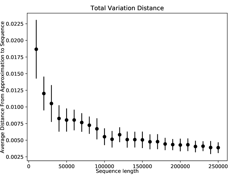
Figure 1: This figure represents the average difference between a non-graphic sequence selected from a power-law distribution with exponent of 2 and its approximation created from Algorithm 1. Each point represents the average distance for 30 sequences created at a given length. The error bars represent one standard deviation.

Theorem 5.

Let $\mathcal{F}$ be a family of integer sequences where for any $\alpha\in\mathcal{F}$ whose sum is $s$ and length is $n$, then $s=o(n^{2})$. For $\alpha\in\mathcal{F}$,

$$\lim_{n\rightarrow\infty}TV(P(\alpha),P(\alpha\wedge T(n,s)))=0.$$ (10)

Proof.

From the definition of the sequence $T$, the number of non-zero entries it contains is $m$. From the definition of the meet operation, the values for the sequence $T\wedge\alpha$ will be equal to $\alpha_{i}$ for all indices $i>m$. It follows from Theorem 4, that a simple upper bound on $m$ is $\sqrt{s}$. Thus an upper bound on the possible change in the probability of any one value in the distribution is

$$\sup_{\omega}|P(\alpha)_{\omega}-P(\alpha\wedge T(n,s))_{\omega}|\leq\frac{m}{n}<\frac{\sqrt{s}}{n}.$$ (11)

Since $s=o(n^{2})$, then it follows

$$\lim_{n\rightarrow\infty}TV(P(\alpha),P(\alpha\wedge T(n,s)))\leq\lim_{n\rightarrow\infty}\frac{\sqrt{s}}{n}=0,$$ (12)

completing the argument. ∎

This convergent behavior is shown in Figure 1. In this example, for each point, 30 non-graphic sequences with even sum were drawn from a power-law distribution with exponent 2 and the average distance to their approximation was computed. We see that the average total variation distance between the original sequences and their approximations approach zero as the sequence length grows.

5 Conclusions

We give a simple and extremely fast method for approximating a non-graphic sequence with a graphic one. This approach is particularly well-suited for large sequences, since only one-pass through the sequence is needed, and the probability distances are reduced as the sequences become larger. This presents a practical algorithm for large network modeling applications.

References

- [1] A. A. Hagberg, D. A. Schult, and P. J. Swart (2008). “Exploring network structure, dynamics, and function using NetworkX”. In Proceedings of the 7th Python in Science Conference (SciPy2008), pp. 11–15. Pasadena, CA USA.
- [2] M. Mihail and N. Vishnoi (2002). “On generating graphs with prescribed degree sequences for complex network modeling applications”. In Proceedings of the 3rd Workshop on Approximation and Randomization Algorithms in Communication Networks (ARACNE), pp. 1–11.
- [3] P. Hell and D. Kirkpatrick (2009). “Linear-time certifying algorithms for near-graphical sequences”. Discrete Math. 309 (18), 5703–5713. http://dx.doi.org/10.1016/j.disc.2008.05.005.
- [4] Y. C. Chen (1988). “A short proof of Kundu’s -factor theorem”. Discrete Math. 71 (2), 177–179. http://dx.doi.org/10.1016/0012-365X(88)90070-2.
- [5] T. Brylawski (1973). “The lattice of integer partitions”. Discrete Math. 6, 201–219. http://dx.doi.org/10.1016/0012-365X(73)90094-0.
- [6] E. Ruch and I. Gutman (1979). “The branching extent of graphs”. Journal of Combinatorics, Information, & System Sciences 4 (4), 285–295.
- [7] B. Pittel (1999). “Confirming two conjectures about the integer partitions”. Journal of Combinatorial Theory, Series A 88 (1), 123–135. http://dx.doi.org/10.1006/jcta.1999.2986.
- [8] N. Mahadev and U. Peled (1995). Threshold Graphs and Related Topics. North Holland. Annals of Discrete Mathematics 56.
- [9] B. Cloteaux (2015). “Is this for real? Fast graphicality testing”. Computing in Science & Engineering 17 (6), 91–95. http://dx.doi.org/10.1109/MCSE.2015.125.