Viscoelastic subdiffusion in a random Gaussian environment

Abstract

Viscoelastic subdiffusion governed by a fractional Langevin equation is studied numerically in a random Gaussian environment modeled by stationary Gaussian potentials with decaying spatial correlations. This anomalous diffusion is archetypal for living cells, where cytoplasm is known to be viscoelastic and a spatial disorder also naturally emerges. We obtain some first important insights into it within a model one-dimensional study. Two basic types of potential correlations are studied: short-range exponentially decaying and algebraically slow decaying with an infinite correlation length, both for a moderate (several $k_{B}T$, in the units of thermal energy), and strong (5-10 $k_{B}T$) disorder. For a moderate disorder, it is shown that on the ensemble level viscoelastic subdiffusion can easily overcome the medium’s disorder. Asymptotically, it is not distinguishable from the disorder-free subdiffusion. However, a strong scatter in single-trajectory averages is nevertheless seen even for a moderate disorder. It features a weak ergodicity breaking, which occurs on a very long yet transient time scale. Furthermore, for a strong disorder, a very long transient regime of logarithmic, Sinai-type diffusion emerges. It can last longer and be faster in the absolute terms for weakly decaying correlations as compare with the short-range correlations. Residence time distributions in a finite spatial domain are of a generalized log-normal type and are reminiscent also of a stretched exponential distribution. They can be easily confused for power-law distributions in view of the observed weak ergodicity breaking. This suggests a revision of some experimental data and their interpretation.

I Introduction

The research field of anomalous diffusion and transport Shlesinger (1974); Scher and Montroll (1975); Bouchaud and Georges (1990); ben Avraham and Havlin (2000); Hughes (1995); Bouchaud et al. (1990); Bouchaud (1992); Metzler and Klafter (2000); Klafter et al. (2011); Goychuk (2012a); Metzler et al. (2014) currently flourishes getting ever more experimental support and manifestations in such diverse research areas as transport processes in living cells and polymeric solutions Mason and Weitz (1995); Amblard et al. (1996); Saxton and Jacobsen (1997); Waigh (2005); Seisenberger et al. (2001); Caspi et al. (2002); Weiss et al. (2004); Tolic-Norrelykke et al. (2004); Banks and Fradin (2005); Barkai et al. (2012); Bruno et al. (2011, 2009); Golding and Cox (2006); Guigas et al. (2007); Szymanski and Weiss (2009); Höfling and Franosch (2013); Jeon et al. (2011); Luby-Phelps (2013); Pan et al. (2009); Wong et al. (2004); Harrison et al. (2013); Parry et al. (2014); Robert et al. (2010); Bruno et al. (2011, 2009); Goychuk et al. (2014a, b); Goychuk (2015a); Tabei et al. (2013); Weigel et al. (2011); Weiss (2013); Santamaria-Holek et al. (2007); Bertseva et al. (2012), colloidal systems Mason and Weitz (1995); Waigh (2005); Evers et al. (2013); Hanes et al. (2013), dust plasmas Nunomura et al. (2006), organic photoconductors Schubert et al. (2013), conformational diffusion in proteins Yang et al. (2003); Kou and Xie (2004); Goychuk and Hänggi (2004); Kneller and Hinsen (2004); Min et al. (2005); Calandrini et al. (2010); Calligari et al. (2011, 2015); Goychuk (2015b); Hu et al. (2016), self-diffusion in lipid bilayers Kneller et al. (2011); Jeon et al. (2012, 2016), diffusion of proteins on DNA strands Kong et al. (2016); Kong and Houten (2017); Liu et al. (2017), to name just a few. Differently from normal diffusion, $\alpha=1$, the variance of the diffusing particle positions, $\langle\delta x^{2}(t)\rangle\propto t^{\alpha}$, often grows sublinearly, $\alpha<1$, or superlinearly, $\alpha>1$, in time, with some power law exponent $\alpha$. Accordingly, anomalous diffusion is classified into the subdiffusion, $\alpha<1$, and the superdiffusion, $\alpha>1$. This classification is, however, not complete. For example, Sinai diffusion Sinai (1982); Bouchaud and Georges (1990); ben Avraham and Havlin (2000) is characterized by a logarithmically slow growth, $\langle\delta x^{2}(t)\rangle\propto\ln^{4}t$. This is clearly a sub-diffusion, which sometimes is named ultraslow Bouchaud and Georges (1990); ben Avraham and Havlin (2000). The research field of anomalous diffusion remains rather controversial because one and the same phenomena are often described by very different theories Goychuk (2012a); Goychuk and Hänggi (2011), such as continuous time random walks (CTRWs) with a divergent mean residence time in local traps Shlesinger (1974); Scher and Montroll (1975); Bouchaud and Georges (1990); ben Avraham and Havlin (2000); Hughes (1995); Metzler and Klafter (2000), and generalized Langevin dynamics with sub-Ohmic memory friction Weiss (1999); Pottier (2003); Kupferman (2004); Goychuk (2009, 2012a). Such different theories of fractional diffusion and transport can look at first very similar Goychuk and Hänggi (2011). However, a deeper analysis reveals fundamental differences in ergodic vs. weakly non-ergodic behavior Bouchaud (1992); Metzler et al. (2014), major features of nonlinear diffusion and transport in tilted periodic potentials Goychuk et al. (2006); Heinsalu et al. (2006); Goychuk (2009, 2012a); Goychuk and Hänggi (2011), as well as in response to external time-periodic modulations Barbi et al. (2005); Sokolov and Klafter (2006); Heinsalu et al. (2007a, 2009); Goychuk (2007, 2012a, 2014).

The pertinent diffusion in cytosol of biological cells is three-dimensional, and one in the cell plasma membrane is two-dimensional. However, the insights obtained from simplified one-dimensional theoretical models proved their usefulness over the years of research Shlesinger (1974); Scher and Montroll (1975); Bouchaud and Georges (1990); ben Avraham and Havlin (2000); Hughes (1995); Metzler and Klafter (2000). Hence, in this paper we will concentrate on a very simplified, minimal 1d model, which, nevertheless, is rich and complex enough. It suits well for getting such important insights and is based on two theoretical approaches to anomalous diffusion, which are especially important in view of their profound dynamical origin. One is based on the Bogolyubov-Ford-Kac-Mazur-Kubo-Zwanzig Bogolyubov (1945); Ford et al. (1965); Kubo (1966); Zwanzig (1973) generalized Langevin equation (GLE)

$$m\ddot{x}+\int_{0}^{t}\eta(t-t^{\prime})\dot{x}(t^{\prime})dt^{\prime}=f(x,t)+\xi(t),$$ (1)

for the particle position $x(t)$ with an algebraically decaying memory kernel $\eta(t)\propto t^{-\alpha}$ Wang and Tokuyama (1999); Lutz (2001); Pottier (2003); Goychuk and Hänggi (2007); Goychuk (2009, 2012a). Another one relies on normal, memory-less Langevin diffusion in random potentials Bouchaud and Georges (1990); Bouchaud et al. (1990). In Eq. (1), $m$ is the mass of the particle, $f(x,t)=-\partial U(x,t)/\partial x$ is an external force acting on the particle, which can be random, both in space and in time, and $\xi(t)$ is an equilibrium thermal noise with zero mean value. It has a Gaussian statistics and hence is named Gaussian. As any zero-mean stationary Gaussian process, it is completely characterized by its autocorrelation function (ACF), $\langle\xi(t)\xi(t^{\prime})\rangle$. This one is related to the memory kernel $\eta(t)$ by the classical fluctuation-dissipation relation (FDR), $\langle\xi(t)\xi(t^{\prime})\rangle=k_{B}T\eta(|t-t^{\prime}|)$ Kubo (1966); Zwanzig (1973); Weiss (1999), named also the second fluctuation-dissipation theorem (FDT) by Kubo Kubo (1966). Here, $T$ is temperature and $k_{B}$ is the Boltzmann constant. Standard Langevin equation presents a particular memory-less case with $\eta(t)=2\eta_{0}\delta(t)$, where $\eta_{0}$ is a viscous friction coefficient, yielding $\eta_{0}\dot{x}$ for the friction term in (1).

There are many studies of GLE dynamics, both potential-free and in some regular potentials, as well as of normal Langevin dynamics in random potentials. However, viscoelastic GLE subdiffusion in random potentials presents currently a practically unexplored topic despite its obvious relevance for diffusion processes in cytosol of living cells and other inhomogeneous viscoelastic media. Only in a parabolic weakly corrugated trapping potential such a diffusion was partially addressed recently Duan and Liang (2012). This is the main purpose of this paper to do the first systematic study of viscoelastic GLE subdiffusion in stationary Gaussian potentials $U(x)$ with decaying correlations. We shall investigate two such models of general interest: (i) with exponentially decaying correlations (Ornstein-Uhlenbeck process in space), and (ii) algebraically decaying correlations possessing no effective correlation length.

Starting from classical works by Bogolyubov Bogolyubov (1945), Ford, Kac, Mazur Ford et al. (1965), and Zwanzig Zwanzig (1973), the GLE (1) has repeatedly been derived Lindenberg and Seshardi (1981); Ford et al. (1988); Kupferman (2004); Weiss (1999); Goychuk (2012a) from a fully dynamical system, where the environment is modeled by a large system of harmonic oscillators forming a thermal bath. The only non-dynamical element, which enters this theory, is that the initial positions and momenta of those oscillators are canonically distributed at a given fixed temperature. In this respect, this dynamical theory of Brownian motion presents a precursor and companion of molecular dynamics Alder and Wainwright (1957, 1967), in a very simplified, model fashion. It is also easy to generalize towards quantum-mechanical Brownian motion Magalinskii (1959); Caldeira and Leggett (1983); Ford et al. (1988); Weiss (1999) and to nonlinear models of coupling between the Brownian particle and its linear environment Lindenberg and Seshardi (1981); Weiss (1999). The influence of the environment in this approach is fully characterized by its spectral density Caldeira and Leggett (1983); Ford et al. (1988); Weiss (1999), $J(\omega)$. It yields the memory kernel as Weiss (1999); Goychuk (2012a) $\eta(t)=(2/\pi)\int_{0}^{\infty}d\omega J(\omega)\cos(\omega t)/\omega$. Here, a very insightful basic model is $J(\omega)=\eta_{\alpha}|\sin(\pi\alpha/2)|\omega^{\alpha}\exp(-\omega/\omega_{c})$Caldeira and Leggett (1983); Ford et al. (1988); Weiss (1999). In accordance with it, the environment is customarily classified by the low-frequency behavior of $J(\omega)$ as Ohmic ($\alpha=1$), sub-Ohmic ($0<\alpha<1$) and super-Ohmic ($\alpha>1$) Weiss (1999). Here, $\eta_{\alpha}$ is a fractional friction coefficient and $\omega_{c}$ is a frequency cutoff. It must be present in any condensed medium beyond the continuous medium approximation, which is, however, often used. This spectral model yields Goychuk (2012a); Siegle et al. (2011)

$$\eta(t) = \eta_{\alpha}\frac{|\sin(\pi\alpha/2)|}{\pi/2}\Gamma(\alpha){\rm Re}(it+1/\omega_{c})^{-\alpha}$$

$$= \eta_{\alpha}\frac{|\sin(\pi\alpha/2)|}{\pi/2}\frac{\Gamma(\alpha)\omega_{c}^{\alpha}}{(1+\omega_{c}^{2}t^{2})^{\alpha/2}}\cos[\alpha\arctan(\omega_{c}t)],\;$$

where $\Gamma(z)$ is special gamma-function. Asymptotically, in the limit $t\to\infty$, and for the potential-free diffusion, this model yields $\langle\delta x^{2}(t)\rangle\propto t^{\alpha}$, for $0<\alpha<2$. It covers both sub- and super-diffusion. For $\alpha>2$, diffusion is ballistic Weiss (1999), $\langle\delta x^{2}(t)\rangle\propto t^{2}$. In the singular limit, with unbounded energy spectrum, $\omega_{c}\to\infty$, and in neglecting quantum effects, the Ohmic model leads exactly Weiss (1999) to the standard classical Langevin equation with viscous friction and thermal white Gaussian noise, which are related by the FDR.

By the same token, the sub-Ohmic model in the singular limit $\omega_{c}\to\infty$ leads to a subdiffusive fractional Langevin equation (FLE) Mainardi and Pironi (1996); Lutz (2001); Pottier (2003); Kupferman (2004); Goychuk and Hänggi (2007); Goychuk (2012a). It is a GLE (1) with an algebraically decaying memory kernel, $\eta(t)=\eta_{\alpha}t^{-\alpha}/\Gamma(1-\alpha)$. The corresponding frictional term with memory in Eq. (1) can be abbreviated as $\eta_{\alpha}d^{\alpha}x/dt^{\alpha}$ Caputo (1967); Gorenflo and Mainardi (1997); Mathai and Haubold (2017) using the notion of Caputo fractional derivative, $\frac{{\rm d}^{\alpha}x}{{\rm d}t^{\alpha}}:=\int_{0}^{t}(t-t^{\prime})^{-\alpha}\dot{x}(t^{\prime})dt^{\prime}/\Gamma(1-\alpha)$. Thermal noise entering this FLE is a fractional Gaussian noise (fGn) Mandelbrot and van Ness (1968). This model of subdiffusion and its further generalizations emerge naturally in the context of anomalous diffusion in complex viscoelastic media such as complex liquids, including dense polymeric solutions, dust plasmas, colloids, etc., with a prominent application to anomalous diffusion in cytosol of biological cells, as well as in intrinsic conformational dynamics of proteins.

Likewise, the super-Ohmic model with $1<\alpha<2$ leads to a superdiffusive GLE with a sign-changing and mostly negative memory kernel Mainardi and Pironi (1996); Goychuk (2012a); Siegle et al. (2011). Its integral is always positive and tends to zero with the upper limit of integration (vanishing integral friction). Its absolute value also decays algebraically slow asymptotically. All these features can be understood from Eq. (I). For $1<\alpha<2$, the sign changes at $t_{c}=\tan(\pi/(2\alpha))/\omega_{c}$. The limit $\omega_{c}\to\infty$ is singular, $t_{c}\to 0+$, and for $t>0$, $\eta(t)=-\eta_{\alpha}t^{-\alpha}/|\Gamma(1-\alpha)|$. It must be handled with care because $\eta(t)$ is not a function but distribution in this limit. Then, the corresponding integral term in (1) can be short-handed Mainardi and Pironi (1996); Goychuk (2012a); Siegle et al. (2011) as $\eta_{\alpha}\sideset{{}_{0}}{{}_{t}}{\mathop{\hat{D}}^{\alpha-1}}\dot{x}(t)$ using the notion of fractional Riemann-Liouville derivative Mathai and Haubold (2017), $\sideset{{}_{0}}{{}_{t}}{\mathop{\hat{D}}^{\gamma}}v(t):=\frac{1}{\Gamma(1-\gamma)}\frac{d}{dt}\int_{0}^{t}dt^{\prime}\frac{v(t^{\prime})}{(t-t^{\prime})^{\gamma}}$, with $\gamma=\alpha-1$ and $v=\dot{x}$.

Such a related FLE, describing, however, an asymptotically normal diffusion, captures hydrodynamic memory effects by Boussinesq and Basset Landau and Lifshitz (1987). It takes the form of Eq. (1) with the frictional term abbreviated as $\eta_{0}\dot{x}+\eta_{\alpha}\sideset{{}_{0}}{{}_{t}}{\mathop{\hat{D}}^{\alpha-1}}\dot{x}(t)$ and two corresponding FDR-related noise terms Mainardi and Pironi (1996). These memory effects lead to a famous long tail in the velocity ACF of Brownian particles even in simple fluids Alder and Wainwright (1967); Mainardi and Pironi (1996); Siegle et al. (2011); Goychuk (2012a). Experimental manifestations of such effects for Brownian particles were found quite recently Huang et al. (2011); Franosch et al. (2011).

The GLE approach naturally provides a dynamical underpinning and justification of the mathematical model of fractional Brownian motion (fBm) by Kolmogorov Kolmogorov (1940, 1991), Mandelbrot and van Ness Mandelbrot and van Ness (1968) within the FLE description upon neglecting the inertial effects. This dynamical origin and consistency with thermodynamics and equilibrium statistical physics for undriven dynamics make this approach superior to many others in the field of anomalous diffusion Goychuk (2012a). One of its special advantages is that it allows to study nonlinear anomalous dynamics in external multistable potentials. For example, such bistable subdiffusive dynamics was studied in Ref. Goychuk (2009) with a prominent result that the residence time distributions (RTDs) in the potential wells are of the stretched exponential type. In fact, no genuine rate description is possible. This is due to the presence of slow fluctuations in the medium such that relatively fast escape events from one potential well to another can occur on the background of very sluggish, quasi-static fluctuations of the environment. Such fluctuations make the whole setup very different from one of the classical rate theory. The latter one assumes that the intrawell relaxation occurs much faster than the escape events. This basic assumption is fundamentally broken for viscoelastic subdiffusive escape, where the slow modes of viscoelastic environment result into a time-modulation of the escape rate formed by the relatively faster relaxation modes. However, a characteristic time scale of transitions nevertheless exists. It is clearly seen in the distribution of the logarithmically-transformed residence times, where the maximum of distribution is well reproduced Goychuk (2009, 2012a, 2015b) from a rate expression of the non-Markovian rate theory Grote and Hynes (1980); Hänggi et al. (1990). It depends in the Arrhenius manner on the height of potential barrier.

Next, the viscoelastic GLE subdiffusion in a washboard potential was shown to be insensitive asymptotically to the presence of potential Goychuk (2009). It approaches gradually a free-subdiffusion limit Goychuk (2009, 2012a); Goychuk and Hänggi (2011) for any barrier height. This astounding feature is in a sharp contrast with both the intuition and well-known results on normal diffusionHänggi et al. (1990) and fractional Fokker-Planck (FFP) dynamics Goychuk et al. (2006); Heinsalu et al. (2006) in washboard potentials. It was also demonstrated for diffusion and transport in other tilted periodic potentials including ratchets potentials with broken space inversion symmetry Goychuk (2012a); Goychuk and Hänggi (2011). Within a quantum-mechanical setting, it has been proven exactly, however, for strictly sinusoidal potentials only Weiss (1999); Chen and Lebowitz (1992). In fact, it is not caused by quantum-mechanical effects at all, as one might possibly believe, and it is not restricted by sinusoidal potentials only Goychuk (2012a). In this respect, it is also important to mention that the potential-free viscoelastic diffusion is ergodic: the ensemble and single-trajectory averages coincide Goychuk (2009), in a sharp contrast e.g. with continuous time random walk (CTRW) semi-Markovian subdiffusion He et al. (2008); Lubelski et al. (2008); Metzler et al. (2014). However, imposing a periodic potential makes it transiently non-ergodic Goychuk (2009). These earlier results are very important to understand some of the key findings of this study.

Another important approach to anomalous diffusion is based on normal diffusion in random potentials Bouchaud and Georges (1990); Bouchaud et al. (1990); Hughes (1995). Such a description naturally emerge in inhomogeneous disordered materials, including viscoelastic cytosol of living cells as well. This is also a very rich and versatile approach. For example, the model of exponentially distributed energy disorder with root-mean-square (rms) amplitude of fluctuations $\sigma$ leads in a mean-field approximation to CTRW subdiffusion with a power law RTD, $\psi(\tau)\propto\tau^{-1-\alpha},0<\alpha=k_{B}T/\sigma<1$, in local traps Hughes (1995). It is featured by divergent mean residence times (MRTs) Scher and Montroll (1975); Shlesinger (1974) and is (weakly) nonergodic Bouchaud (1992); Bel and Barkai (2005); Lubelski et al. (2008); He et al. (2008); Barkai et al. (2012); Sokolov et al. (2009): The ensemble and trajectory averages are radically different.

However, in random potentials presenting stationary Gaussian processes in space such a diffusion is asymptotically normal for any decaying correlations in spaceGoychuk and Kharchenko (2014), i. e. $\alpha(t)\to 1$, for $t\to\infty$. Here, a prominent result by de Gennes, Bässler, and Zwanzig holds on the renormalized normal diffusion coefficient, $D_{\rm ren}=D_{0}\exp[-\sigma^{2}/(k_{B}T)^{2}]$, where $D_{0}$ is the potential-free diffusion coefficient Gennes (1975); Bässler (1987, 1993); Zwanzig (1988). The same renormalization is valid for FFP dynamics in such potentials, $\langle\delta x^{2}(t)\rangle\propto D_{\rm ren}t^{\alpha}$, where $D_{0}$ must be treated as fractional diffusion coefficient, see in Appendix A. The corresponding temperature dependence is often measured in disordered materials Hecksher et al. (2008) and the Gaussian model of energy disorder is physically well justified in many cases, e.g. for diffusion of electrons and holes in organic photoconductors Bässler (1993); Dunlap et al. (1996), colloidal particles in random laser fields Evers et al. (2013); Bewerunge and Egelhaaf (2016); Hanes et al. (2013) and regulatory proteins on DNA tracks Gerland et al. (2002); Lässig (2007); Slutsky et al. (2004); Bénichou et al. (2009); Goychuk and Kharchenko (2014). However, for a sufficiently strong disorder $\sigma>2k_{B}T$ long subdiffusive transients occur on a mesoscale Romero and Sancho (1998); Khoury et al. (2011); Simon et al. (2013); Goychuk and Kharchenko (2014) with a time-dependent sub-diffusion exponent $\alpha(t)\propto\log(t)$ Goychuk et al. (2017). For $\sigma>(4-5)k_{B}T$, this mesoscale subdiffusion can reach even the macroscale Goychuk and Kharchenko (2014), and $\alpha(t)$ can be nearly constant for a very long time Goychuk and Kharchenko (2014); Goychuk et al. (2017). Remarkably, in this regime it exhibits the same temperature dependence, $\alpha\propto k_{B}T/\sigma$, as in the case of exponential disorder, despite a very different physical mechanism Goychuk et al. (2017). Such transient subdiffusion also exhibits a strong scatter in single-trajectory averagesGoychuk and Kharchenko (2014) featuring a weak ergodicity breaking Lubelski et al. (2008); He et al. (2008); Barkai et al. (2012); Metzler et al. (2014); Krapf et al. (2018); Dean et al. (2016).

Gaussian disorder characterized by a stationary random force $f(x)$ or a random drift coefficient Sinai (1982) is generally very different from the stationary potential disorder. It is also very important in applicationsBouchaud and Georges (1990). Here, the simplest model is given Bouchaud and Georges (1990) by the uncorrelated force disorder, $\langle f(x)f(x^{\prime})\rangle\propto\delta(x-x^{\prime})$, which leads to a logarithmically slow subdiffusion Sinai (1982); Bouchaud and Georges (1990), $\langle\delta x^{2}(t)\rangle\propto\log^{a}(t)$ with $a=4$ Bouchaud and Georges (1990). It is named Sinai diffusion. The corresponding Gaussian potential $U(x)$ is a non-stationary random process. It presents an unbounded Brownian motion (Wiener process) occurring in space, rather than time. If the potential presents a fBm in space, a generalized Sinai diffusion with $a\neq 4$ emerges Oshanin et al. (2013). Astoundingly, a generalized Sinai diffusion emerges also transiently in stationary correlated Gaussian potentials for a sufficiently strong disorder, $\sigma>5k_{B}T$. This has been shown recently for four different models of disorder correlations in Ref. Goychuk et al. (2017), where also the genuine mechanism of the discussed transient subdiffusion has been clarified using a scaling theory argumentation.

This paper is devoted to overdamped viscoelastic subdiffusion in random environments modeled by stationary random potentials with Gaussian statistics. The rest of the paper is organized as follows. In Sec. II, we formulate the model and the numerical approach. In Sec. III, we present the main results and their discussion. Finally, in Sec. IV, the main conclusions will be drawn.

II Model and numerical approach

We consider one-dimensional viscoelastic subdiffusion governed by the following overdamped subdiffusive FLE Goychuk (2012a); Kharchenko and Goychuk (2013); Goychuk (2015b)

$$\eta_{0}\frac{{\rm d}x}{{\rm d}t}+\eta_{\alpha}\frac{{\rm d}^{\alpha}x}{{\rm d}t^{\alpha}}=f(x)+\xi_{0}(t)+\xi_{\alpha}(t),$$ (3)

where $0<\alpha<1$. The particles are moving in a random potential $U(x)$ yielding static random force $f(x)=-dU(x)/dx$. They are also subjected to thermal Gaussian forces $\xi_{0}(t)$ and $\xi_{\alpha}(t)$, as well as a memoryless Stokes friction with the friction coefficient $\eta_{0}$ and a friction with memory or frequency-dependent friction, which is characterized by the fractional friction coefficient $\eta_{\alpha}$, as detailed in the Introduction. Thermal noises and the corresponding frictional parts are related by the FDT relations $\langle\xi_{0}(t)\xi_{0}(t^{\prime})\rangle=2k_{B}T\eta_{0}\delta(t-t^{\prime})$, and $\langle\xi_{\alpha}(t)\xi_{\alpha}(t^{\prime})\rangle=k_{B}T\eta_{\alpha}|t-t^{\prime}|^{-\alpha}/\Gamma(1-\alpha)$, correspondingly. This ensures statistical equilibrium description in the absence of driving forces Kubo (1966). The both noises, $\xi_{\alpha}(t)$ and $\xi_{0}(t)$, present singular stochastic processes with infinite variance. In the language of spectral bath functions, this description corresponds to $J(\omega)=\eta_{0}\omega+\eta_{\alpha}|\sin(\pi\alpha/2)|\omega^{\alpha}$, i.e. a mixture of Ohmic and sub-Ohmic thermal baths Weiss (1999), in the singular limit $\omega_{c}\to\infty$. In the case of cytosol or complex polymeric liquids, the Stokes friction accounts for the water component of solution, whereas the friction with memory is caused by various dissolved polymers forming e.g. actin meshwork. We neglect the inertial effects in anomalous dynamics, which can also be easily included Goychuk (2009, 2012a), because we wish to arrive at a largest possible time scale accessible in numerical simulations. Moreover, very often such effects can indeed be neglected on physical grounds, see Appendix B for a justification. Hydrodynamic memory effects are also neglected, as usually.

The solution of Eq. (3) for free subdiffusion, $f(x)=0$, yields Kharchenko and Goychuk (2013)

$$\langle\delta x^{2}(t)\rangle=2D_{0}tE_{1-\alpha,2}[-(t/\tau_{0})^{1-\alpha}],$$ (4)

where $E_{a,b}(z):=\sum_{0}^{\infty}z^{n}/\Gamma(an+b)$ is generalized Mittag-Leffler function Mathai and Haubold (2017), $D_{0}=k_{B}T/\eta_{0}$ is a normal diffusion coefficient, and $\tau_{0}=(\eta_{0}/\eta_{\alpha})^{1/(1-\alpha)}$ is a transient time constant. Initially, for $t\ll\tau_{0}$, diffusion is normal, $\langle\delta x^{2}(t)\rangle\approx 2D_{0}t$, and asymptotically, $t\gg\tau_{0}$, it is anomalously slow, $\langle\delta x^{2}(t)\rangle\sim 2D_{\alpha}t^{\alpha}/\Gamma(1+\alpha)$, with anomalous diffusion coefficient $D_{\alpha}=k_{B}T/\eta_{\alpha}$. In the particular case of $\alpha=1/2$, Eq. (4) yields

$$\langle\delta x^{2}(t)\rangle = 2D_{1/2}\Bigg{\{}2\sqrt{\frac{t}{\pi}}$$ (5)

$$+ \sqrt{\tau_{0}}\left[e^{t/\tau_{0}}{\rm erfc}\left(\sqrt{\frac{t}{\tau_{0}}}\right)-1\right]\Bigg{\}},$$

which is used to test numerical solutions below.

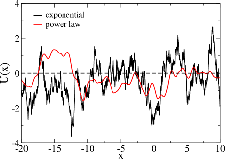
Figure 1: (Color online) Realizations of random potentials (energy in units of $\sigma$, and coordinate in units of $\lambda$) for exponential and power law correlations. The lattice grid size is $\Delta x=0.02$. In the case of power-law correlations, $\gamma=0.8$.

We consider stationary zero-mean random Gaussian potentials, which are completely characterized by the normalized stationary autocorrelation function, $g(x)=\langle U(x_{0}+x)U(x_{0})\rangle/\langle U^{2}(x)\rangle$, and the rms of fluctuations, $\sigma=\langle U^{2}(x)\rangle^{1/2}$. Two models of correlations are considered: (i) exponential, $g(x)=\exp(-|x|/\lambda)$, and (ii) power law decaying, $g(x)=1/(1+x^{2}/\lambda^{2})^{\gamma/2}$. In the first case, $\lambda$ is the correlation length, $\lambda_{\rm corr}=\int_{0}^{\infty}g(x)dx$, and in the second case $\lambda_{\rm corr}\to\infty$, for $0<\gamma<1$, as e.g. for diffusion of proteins on biological DNAs Peng et al. (1992); ben Avraham and Havlin (2000); Goychuk et al. (2017). Then, $\lambda$ is just a scaling parameter, which is convenient to use to scale distance in numerics. Furthermore, the time will be scaled in the units of $\tau_{r}=(\lambda^{2}\eta_{\alpha}/\sigma)^{1/\alpha}$, $k_{B}T$ in units of $\sigma$, and normal friction coefficient $\eta_{0}$ in units of $\eta_{\alpha}\tau_{r}^{1-\alpha}$.

II.1 Numerical approach

II.1.1 Random potential generation

Random Gaussian potentials are generated on a lattice evenly spaced with a grid size $\Delta x\ll\lambda$, using a spectral method in accordance with the numerical algorithm detailed in Ref. Simon et al. (2012). It requires to use a periodic boundary condition imposed on $U(x)$ with a very large period $L$. The method is based on the fact the power spectrum $S(k)$ of the random process $U(x)$ is obtained by the Fourier transform of its ACF (Wiener-Khinchine theorem). Moreover, it characterizes the absolute values of the amplitudes of the Fourier components $\hat{U}_{k}$ of $U(x)$ in the wave number space, $\langle\hat{U}_{k}\hat{U}_{k^{\prime}}^{*}\rangle=LS(k)\delta_{k,k^{\prime}}$ Papoulis (1991). First, $S(k)$ is obtained from $g(x)$ by a fast Fourier transform (FFT). Next, Fourier transform of a Gaussian process is a Gaussian process Papoulis (1991). This allows to calculate the random wave amplitudes $\hat{U}_{k}$ from a set of independent Gaussian variables based on $S(k)$ and using another FFT. Finally, numerical inversion of the random wave components $\hat{U}_{k}$ to the coordinate space is done with inverse FFT. This yields the random realizations of $U(x)$. The method uses two direct and one inverse FFTs. The quality of the algorithm is checked and controlled by calculating numerically the ACF of the generated $U(x)$ and comparing it with the original ACF. It is impressively good. The readers are referred to Ref. Simon et al. (2012) for further detail.

In our numerics we fix $\Delta x=0.02$, and $L=2^{19}\approx 10^{4}$. Samples of random potentials with different correlations are presented in Fig. 1. Notice a very rough character of the potential fluctuations for exponential correlations. There are many minima and maxima present within a correlation length. This is because this is a singular model of correlations. As a matter of fact, the corresponding force fluctuation $\langle\delta f^{2}(x)\rangle^{1/2}=\sqrt{2/(\Delta x\lambda)}\sigma$ diverges in the limit of $\Delta x\to 0$. This is a crucial point: $\Delta x$ must be finite, on physical grounds in any such singular model Goychuk et al. (2017). Otherwise, local static forces acting on the particle can take very large values for a vanishing $\Delta x\to 0$. Any stochastic Langevin simulation in such a situation is damned to fail, if the time step $\Delta t$ in simulations is not chosen appropriately small: $\Delta t\to 0$ with $\Delta x\to 0$. The smaller $\Delta x$, the smaller $\Delta t$ must be used for Langevin simulations of such singular models of disorder Goychuk and Kharchenko (2014). The model of a delta-correlated potential is physically a model with $U(x)$ values uncorrelated on the lattice sites. However, because of continuity of potential it remains correlated between the sites of the lattice, anyway Goychuk et al. (2017). This is actually the case, where the potential fluctuations have the wildest character, and do not exhibit a local bias, which otherwise is always present because of correlations. In our numerics, we connect the lattice values of potential by parabolic splines, i.e. the potential is locally parabolic and $f(x)$ is piece-wise linear. Notice also that the power-law correlated potential is much smoother and it does not display the discussed singularity in the limit $\Delta x\to 0$.

II.1.2 Approximation of the memory kernel

Our numerical approach to integrate the FLE dynamics is based on approximation of the power-law memory kernel by a sum of exponentials,

$$\eta(t)=\sum_{i=1}^{N}k_{i}\exp(-\nu_{i}t),$$ (6)

i.e. using a Prony series expansion Goychuk (2009); McKinley et al. (2009). Eq. (6) presents a particular case of more general Prony series Prony (1795); Hauer et al. (1990); Park and Schapery (1999); Schapery and Park (1999), $s(t)=\sum_{i=1}^{N}k_{i}\exp(-\nu_{i}t)\cos(\omega_{i}t+\delta_{i})$, used to approximate any empirical signal $s(t)$ using $N$ decaying wave-forms, with decay rates $\nu_{i}$, frequencies $\omega_{i}$, and phase shifts $\delta_{i}$. It presents a further generalization of Fourier series and has been introduced originally by Prony in 1795 Prony (1795). The expansions of viscoelastic memory kernels like one in Eq. (6) naturally emerge in the theory of polymer dynamics and polymeric melts Doi and Edwards (1986). For example, for the Rouse model of a polymer consisting of $N$ monomers Doi and Edwards (1986), $\nu_{i}=i^{p}\nu_{l}$ with $p=2$ and $k_{i}=const$, in terms of some smallest $\nu_{l}$ in the hierarchy of relaxation rates $\nu_{i}$. This yields McKinley et al. (2009) $\eta(t)\propto 1/t^{1/p}$, e.g. $\alpha=1/2$ for $p=2$, in the range of $\tau_{l}\ll t\ll\tau_{h}$, with $\tau_{h}=1/\nu_{l}$, and $\tau_{l}=N^{p}/\nu_{l}=\nu_{0}$. Notice that it is $\nu_{0}$ which plays a fundamental role being related to the overdamped dynamics of one monomer in the Rouse chain Doi and Edwards (1986). It determines the lower time cutoff of the power law dependence $\eta(t)\propto t^{-\alpha}$. Accordingly, $\nu_{l}=\nu_{0}/N^{p}$. The larger $N$, the larger is the upper time cutoff $\tau_{h}=N^{p}/\nu_{0}$, whereas $\tau_{l}$ remains unchanged. Notice that the both time cutoffs naturally emerge in the dynamics of polymeric melts. They always exist.

The polymeric scaling of the relaxation rates $\nu_{i}$ is not unique. Another way is to choose a fractal scaling, $\nu_{i}=\nu_{0}/b^{i-1}$, with the spring constants $k_{i}=C_{\alpha}(b)\nu_{i}^{\alpha}/\Gamma(1-\alpha)\propto\nu_{i}^{\alpha}$, where $C_{\alpha}(b)$ is some constant, which depends on $\alpha$ and $b$ Palmer et al. (1984); Hughes (1995); Goychuk (2009, 2012a). It is used e.g. in a phenomenological temporary network model of polymeric melts Larson (1999). Already for a rather crude scaling with $b=10$, the accuracy of this approximation between two memory cutoffs, $\tau_{l}=1/\nu_{0}$ and $\tau_{h}=\tau_{l}b^{N-1}$, reaches several percents for $\alpha=0.5$ Goychuk (2009). The great advantage of the fractal scaling over the polymeric one is that it is requires a much smaller number $N$ of viscoelastic modes in the memory kernel approximation. Indeed, for having the same range $\tau_{h}/\tau_{l}$ of power law scaling within the polymeric scaling as within the fractal scaling with $N$ terms one needs

$$M=b^{(N-1)/p}\;$$ (7)

terms in (6). For example, for $\alpha=0.5$ and $p=2$ this would give $M=10^{5}$ (!) instead of $N=11$ within the fractal scaling with $b=10$, or $N=35$ with $b=2$. This clearly establishes superiority of the fractal scaling in numerics Goychuk (2012a). It allows for a numerically very efficient approach to integrate FLE Goychuk (2009, 2012a). Notice that $\nu_{0}$ can be chosen somewhat smaller (to avoid numerical instability) than the inverse time step $1/\Delta t$ in the numerical simulation, and even $N\sim 10-20$ is typically sufficient in numerical simulations with $b=10$. For the scaling with $b=2$, the accuracy of the memory kernel approximation improves to $0.01\%$ Goychuk and Kharchenko (2013). Then, however, one should also increase $N$ accordingly, which would provide an extra time burden in the numerics. Accuracy of several percents is normally sufficient.

II.1.3 Markovian embedding

Next, we introduce a subset of auxiliary variables $x_{i}$ Goychuk (2009) corresponding to the viscoelastic modes of the environment. Physically, they can be interpreted as coordinates of some auxiliary Brownian quasi-particles modeling viscoelastic Maxwellian modes of the environment and elastically coupled with spring constants $k_{i}$ to the central Brownian particle Goychuk (2012a). The fractional Gaussian noise $\eta_{\alpha}(t)$ in this approach is approximated by a sum of Ornstein-Uhlenbeck processes with autocorrelation times $1/\nu_{i}$. Very important and even crucial in applications is that this Maxwell-Langevin approach to viscoelastic subdiffusive dynamics allows for a straightforward Markovian embedding Goychuk (2012a):

$$\eta_{0}\dot{x}=f(x)-\sum_{i=1}^{N}k_{i}(x-x_{i})+\sqrt{2k_{B}T\eta_{0}}\zeta_{0}(t),$$ (8a)

$$\eta_{i}\dot{x}_{i}=k_{i}(x-x_{i})+\sqrt{2k_{B}T\eta_{i}}\zeta_{i}(t),$$ (8b)

where $\zeta_{i}(t)$ are $N+1$ uncorrelated white Gaussian noises, $\langle\zeta_{i}(t)\zeta_{j}(t^{\prime})\rangle=\delta_{ij}\delta(t-t^{\prime})$, and $\eta_{i}=k_{i}/\nu_{i}$ are frictional coefficients of auxiliary Brownian particles. This Markovian dynamics in the space of $N+1$ dimensions can be propagated using well-established algorithms like stochastic Euler or stochastic Heun methods Gard (1988) without principal difficulties, with a well controlled numerical accuracy. By excluding the auxiliary variables $x_{i}$ in Eq. (8a), (8b) it is easy to show that the resulting GLE for the coordinate $x$ has indeed the memory kernel, which is presented by the sum of exponentials (6), and the correlated noise term, which is the sum of corresponding Ornstein-Uhlenbeck processes. For this, one has to first rewrite (8b) in terms of the viscoelastic force $u_{i}=k_{i}(x_{i}-x)$, and formally solve the resulting equation for $u_{i}$. This yields

$$u_{i}(t)=-\int_{0}^{t}k_{i}e^{-\nu_{i}(t-t^{\prime})}\dot{x}(t^{\prime})dt^{\prime}+\chi_{i}(t)$$ (9)

with

$$\chi_{i}(t) = u_{i}(0)e^{-\nu_{i}t}$$

$$+ \sqrt{2k_{B}Tk_{i}\nu_{i}}\int_{0}^{t}e^{-\nu_{i}(t-t^{\prime})}\zeta_{i}(t^{\prime})dt^{\prime}.$$

Each noise component $\chi_{i}(t)$ depends on $u_{i}(0)$, and all the noise components are mutually independent. Indeed, considering $u_{i}(0)$ as independent random Gaussian variables with $\langle u_{i}(0)\rangle=0$ and $\langle u_{i}^{2}(0)\rangle=k_{i}k_{B}T$, one can show that $\chi_{i}(t)$ present wide sense stationary Gaussian stochastic processes with $\langle\chi_{i}(t)\chi_{j}(t^{\prime})\rangle=k_{B}Tk_{i}\delta_{ij}e^{-\nu_{i}|t-t^{\prime}|}$. Substituting (9) in (8a) establishes the stated equivalence Goychuk (2009, 2012a), provided that the initial $x_{i}(0)$ in (8b) are random Gaussian variables such that, $\langle x_{i}(0)\rangle=x(0)$, $\langle[x_{i}(0)-x(0)]^{2}\rangle=k_{B}T/k_{i}$. The considered Markovian embedding is exact, when the memory kernel is exactly the sum of exponentials (6).

The whole idea of Markovian embedding is very natural and sound in view of a dynamical origin of GLE dynamics: Instead of considering huge many thermal bath oscillators one replaces them by a handful of overdamped stochastic Brownian oscillators, with a nice physical interpretation in terms of a generalized Maxwell-Langevin theory of viscoelasticity Goychuk (2012a). The efficiency of the resulting numerical approach has a proven record Goychuk (2009, 2010, 2012a); Kharchenko and Goychuk (2012); Goychuk and Kharchenko (2013); Goychuk et al. (2014a, b); Goychuk (2015a). Upon a modification, this method can also be used for Markovian embedding of superdiffusive FLE dynamics Siegle et al. (2010, 2011). Clearly, it can be also considered as an independent approach to anomalous dynamics without any relation to FLE.

In any particular case, one has to choose the embedding parameters appropriately, considering a trade-off between the numerical accuracy and feasibility of simulations on the required time scale. The accuracy is controlled by comparison with the exact results like one in Eqs. (4), (5). In our simulations below we use for $\alpha=0.5$, $b=10$, $\eta_{0}=0.1$, $\nu_{0}=10^{3}$, $N=12$, $C_{0.5}(10)=1.3$, which warrants $3-5\%$ accuracy in numerics. The rms of potential $\sigma$ is fixed in simulations, whereas temperature varies in units of $\sigma/k_{B}$. The time-step of integration was chosen $\Delta t=5\times 10^{-5}$, and the maximal time was $t_{\rm max}=2\times 10^{5}$. Stochastic Heun method (see in Appendix C) was used with double precision on high-performance graphical processors Tesla K20. In the ensemble trajectory simulations, $n=10^{4}$ particles were initially uniformly distributed within $[0,L]$ spatial interval with 10 different potential realizations in each case ($10^{5}$ particles in the ensemble averaging). Random potentials were generated as described above, in accordance with Simon et al. (2012), and simulations were run with periodic boundary conditions. It took typically about 5 days of computational time for each ensemble-averaged curve presented below. The results were first tested against the exact analytical result in Eq. (5) in the absence of random potential. The numerical results coincide in this case with the analytical result within the width of the plotted curves like in Fig. 2, a in Ref. Goychuk (2009), and especially, Figs. 5, 6 in Ref. Goychuk (2012a), Fig. 2 of Goychuk and Kharchenko (2013) and inset of Fig. 1 in Ref. Kharchenko and Goychuk (2013).

III Results and Discussion

III.1 Ensemble averaging

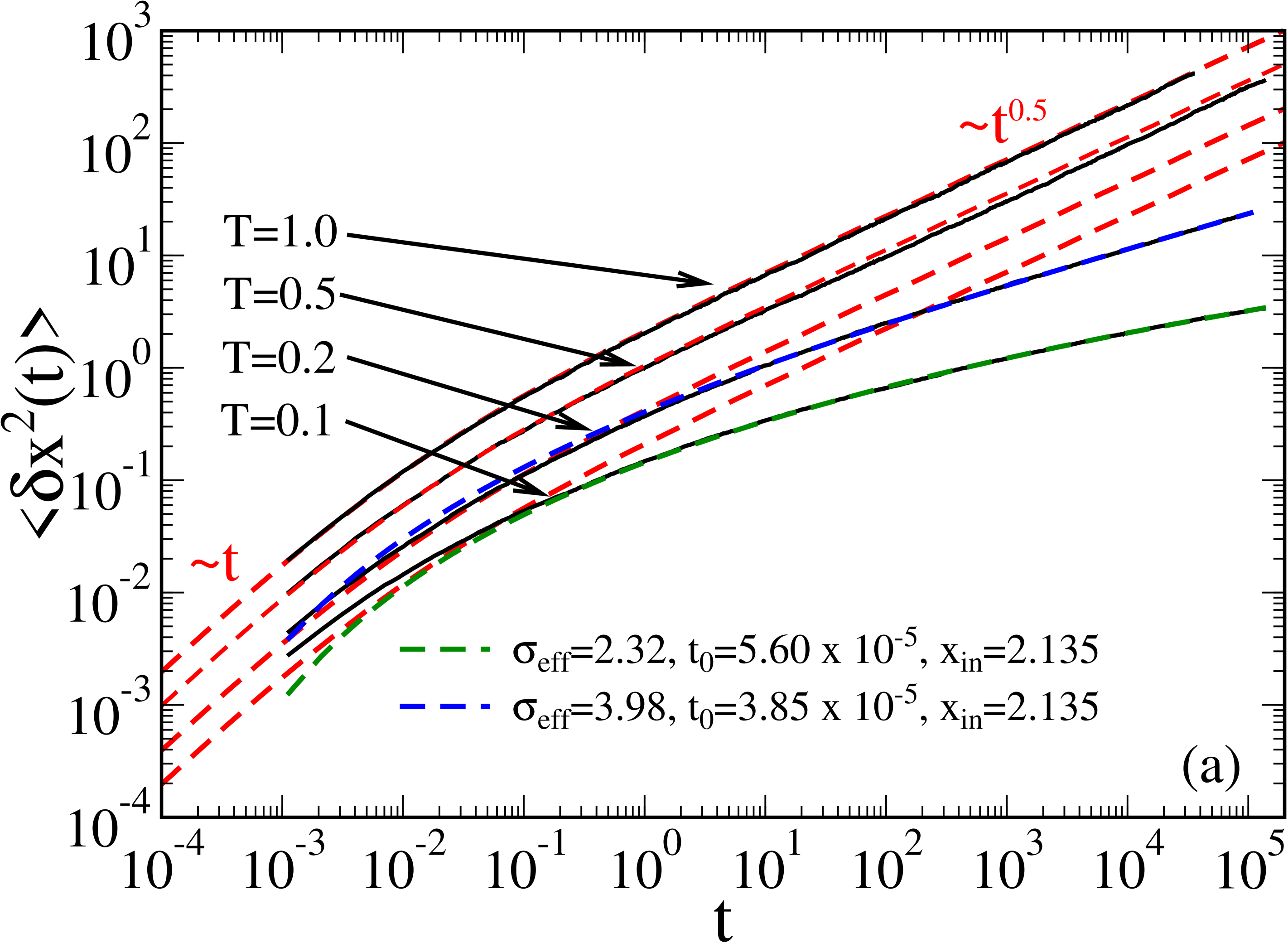
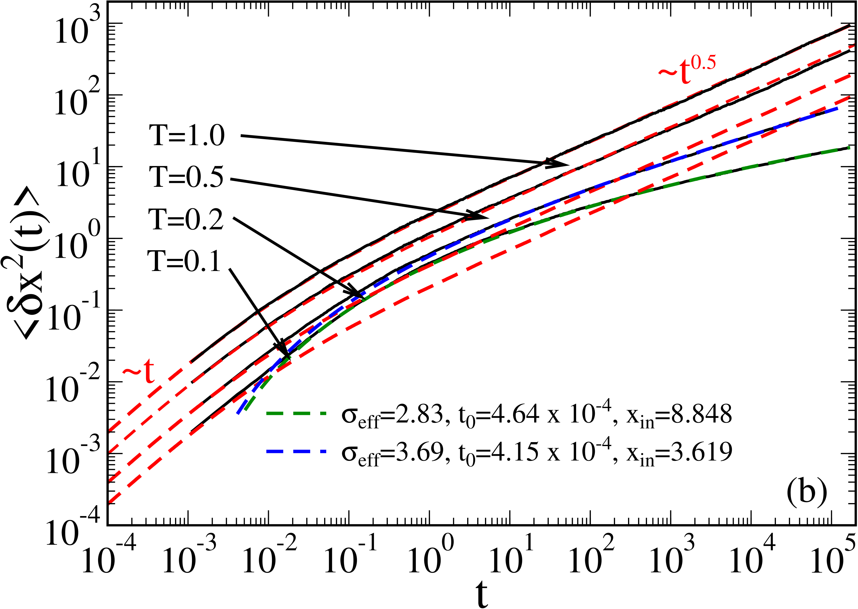
Figure 2: (Color online) Ensemble-averaged mean squared displacement versus time in units of $\tau_{r}=(\lambda^{2}\eta_{\alpha}/\sigma)^{1/\alpha}$ for different values of $k_{B}T$ in units of the disorder strength $\sigma$ for (a) exponential decay of correlations and (b) power-law decay with $\gamma=0.8$. The fit of the numerical results (full black lines) is performed for $T=0.2$ with the expression (12) and for $T=0.1$ using (11). The fitting parameters are shown in the plot. Dashed red lines depict exact results for free subdiffusion in accordance with Eq. (5): $\alpha=0.5$, $\eta_{0}=0.1$ and $\tau_{0}=0.01$.

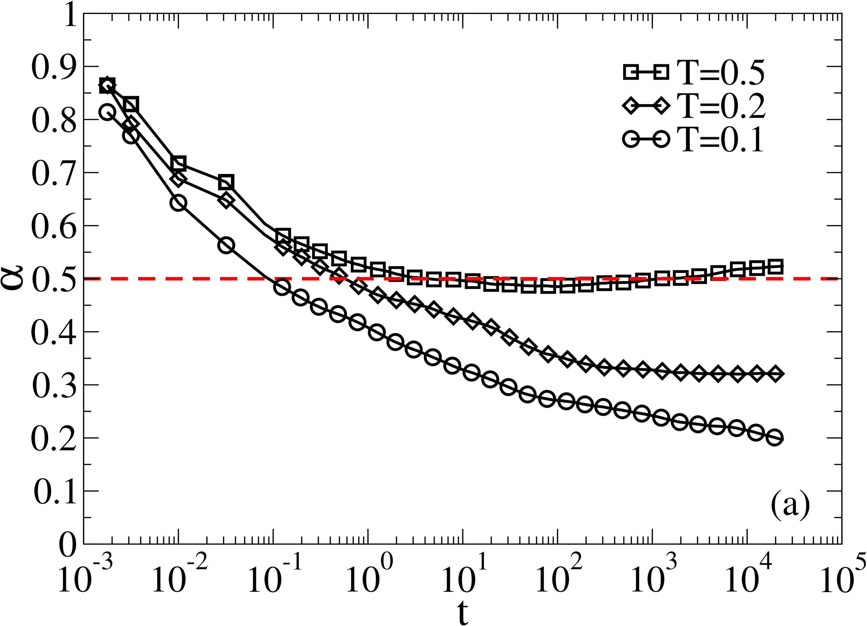
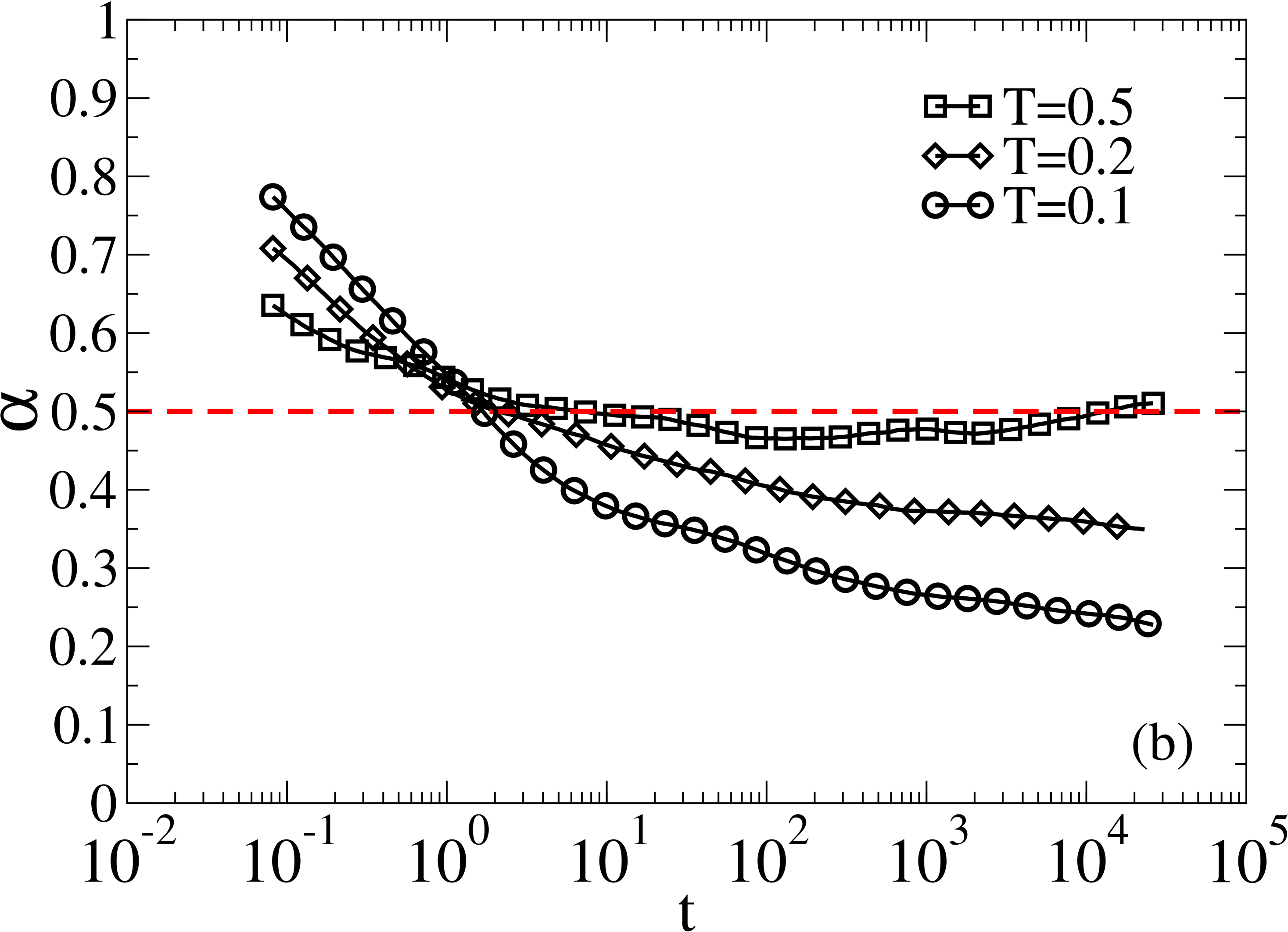
Figure 3: (Color online) Time-dependent power law exponent $\alpha(t)$ for an assumed subdiffusive law $\langle\delta x^{2}(t)\rangle\propto t^{\alpha(t)}$ obtained as the logarithmic derivative of the traces in Fig. 2, for different temperatures in the case of (a) exponential correlations, (b) power law correlations with $\gamma=0.8$.

We first concentrate on the ensemble averaging. The results are shown in Fig. 2 for the exponentially decaying correlations in part (a) and for the power-law decaying correlations with $\gamma=0.8$ in part (b), for several different values of temperature starting from $T=1$ and ending with $T=0.1$. The first striking feature for both types of correlations is that random potential practically does not matter for $T=1$ and the results are not different from the exact result of potential-free subdiffusion depicted by a broken red line in accordance with Eq. (5). This is not a trivial feature at all, even if it could be expected from the earlier results on viscoelastic subdiffusion in periodic potentials Goychuk (2009, 2012a). However, intuition says that a combination of slowness caused viscoelastic effects with sluggishness caused by random potential should result into an ultraslow behavior. This intuition is wrong. Very differently from memoryless diffusion in stationary Gaussian potentials, which is asymptotically normal and exponentially suppressed by disorder, viscoelastic subdiffusion is not suppressed asymptotically by disorder at all, on the ensemble level. This result is very surprising indeed because another fractional dynamics in such random potentials, namely fractional Fokker-Planck dynamics, predicts a very different result, see in Appendix A, $\langle\delta x^{2}(t)\rangle=2D_{\alpha}\exp[-\sigma^{2}/(k_{B}T)^{2}]t^{\alpha}/\Gamma(1+\alpha)$, i.e. the renormalization factor is the same for as for normal diffusion. Especially in the case exponential correlations this result of viscoelastic fractional subdiffusion is very surprising even for $T=1$, as soon one realizes that in this case the amplitude of potential fluctuations can largely exceed $k_{B}T$ well within a distance of the correlation length, see in Fig. 1. However, with the lowering temperature the influence of potential becomes visible already for $T=0.5$, although the potential-free asymptotics is almost reached at the end point of simulations in Fig. 2, and the influence is really small, barely detectable. For $T=0.1$, it becomes very distinct, and the corresponding transient regime lasts indeed very long: No slightest signature of an asymptotic regime is even present in Fig. 2 for $T=0.1$. The corresponding asymptotics is simply impossible to reach numerically. Instead of a power-law subdiffusion, one clearly detects a nominally ultra-slow logarithmic diffusion of the Sinai type:

$$\langle\delta x^{2}(t)\rangle\approx x_{\rm in}^{2}\left[(k_{B}T/\sigma_{\rm eff})\ln(t/t_{0})\right]^{4}$$ (11)

with three fitting parameters: $\sigma_{\rm eff}$, $x_{\rm in}^{2}$, and $t_{0}$, two of which can be combined in the only one, $x_{\rm in}^{2}/\sigma_{\rm eff}^{4}$, in this case. It describes numerics nicely over about $7$ time decades for both types of correlations. For a larger $T=0.2$, numerics are fitted well by a more complex, yet only three parameters dependence Goychuk et al. (2017)

$$\langle\delta x^{2}(t)\rangle=x_{\rm in}^{2}\left\{e^{[(k_{B}T/\sigma_{\rm eff})\ln(t/t_{0})]^{2}}-1\right\}^{2}\;.$$ (12)

It follows from a scaling consideration assuming that a typical time to travel a certain distance $x$ is defined in an Arrhenius manner by the largest potential barrier met on the pathway and the fact that this largest barrier scales as Zhang (1986); Hanes and Egelhaaf (2012); Goychuk et al. (2017)

$$\delta U_{\rm max}\sim 2\sigma\sqrt{2\ln(x/x_{\rm in})}$$ (13)

with the distance. Indeed, let us estimate a typical time $t$ it takes for a particle to travel the distance $x$ starting at $x_{0}$. It is reasonable to assume that on the intermediate time scales, where the presence of potential is very essential, this time is defined, like in the case of normal diffusion, by the largest barrier met on the particle’s way, $t=t_{0}\exp[|\delta U_{\rm max}(x)|/(k_{B}T)]$, where $t_{0}$ is a prefactor. From this scaling ansatz, upon taking (13) into account, we obtain the estimate in (12) with $\sigma_{\rm eff}=2\sqrt{2}\sigma$. Given a very crude character of this estimate, $\sigma_{\rm eff}$ should be considered as a fitting parameter. Like for memoryless diffusion, this result holds also for viscoelastic subdiffusion because a typical mean time to overcome a potential barrier does scale in Arrhenius manner with its height Goychuk (2009, 2012a). Namely this kind of behavior dominates in the transient regime, where the influence of potential on viscoelastic subdiffusion is very essential. Sinai diffusion in Eq. (11) just follows from Eq. (12) as the lowest order expansion in $k_{B}T/\sigma_{\rm eff}$. The fitted values of $\sigma_{\rm eff}$ agree actually fairly well with the theoretical value $\sigma_{\rm eff}=2\sqrt{2}\sigma\approx 2.83\sigma$ Goychuk et al. (2017). The agreement of the fitted values with theoretical value of $x_{\rm in}=\pi\lambda/\sqrt{\gamma}\approx 3.51\lambda$ for $\gamma=0.8$ Goychuk et al. (2017) is also rather good for power law correlated potentials, see especially for $T=0.2$. For singular model with exponential correlations, which predicts $x_{\rm in}=\pi\sqrt{\lambda\Delta x/2}\approx 0.315\sqrt{\lambda}$ for $\Delta x=0.02$, the agreement worsens. Nevertheless, scaling argumentation of Refs. Bouchaud and Georges (1990); Goychuk et al. (2017) works surprisingly good, given its very rough character, also for viscoelastic subdiffusion in random potentials. Notice that in power-law correlated potentials, Sinai-like subdiffusion is essentially faster in absolute terms than one in exponentially correlated potentials. The reason becomes immediately clear from Fig. 1. This is because power-law correlated disorder is much smoother, and the maximal barrier met on the same distance is essentially smaller than in the case of exponential correlations. Furthermore, an interesting transient effect on the ensemble level is that viscoelastic subdiffusion in random potential can be even faster than the potential-free subdiffusion, see for power law correlations and $T=0.1$ in Fig. 2, b. This is because of an alternating local bias felt by each separate particle Goychuk et al. (2017). Such a local bias and the resulting random drift are responsible e.g. for the Golosov phenomenon in the case of genuine Sinai diffusion Golosov (1984); Bouchaud and Georges (1990). Golosov phenomenon describes at the first look paradoxical effect that in an environment with random bias two particles starting nearby do not diffuse strongly apart being subjected to one and the same local bias in the environment Golosov (1984); Bouchaud and Georges (1990). The observed phenomenon is different. However, it has precisely the same physical origin: a strong local bias which alternates randomly its direction. Single-trajectory averages, see below, do not show such a paradoxical feature. Then, subdiffusion is always suppressed by random potential.

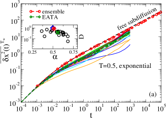
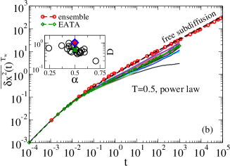
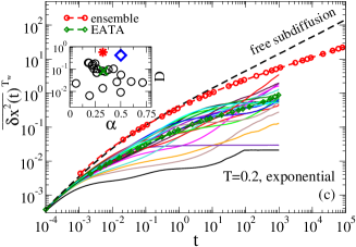
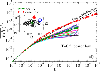
Figure 4: (Color online) Single-trajectory, time-averaged mean squared displacement for two values of temperature $T=0.5$ and $T=0.2$, and two types of correlations shown in each panel. The trajectories time length was ${\cal T}_{\rm w}=10^{5}$. 20 trajectory averages were made for particles starting from different locations. They are depicted with solid lines. The results of the ensemble-averaged, as well as ensemble-averaged time-averaged (EATA), and potential-free subdiffusion are also depicted for comparison. Insets show the distribution of the scaled subdiffusion coefficient $D$ and power law exponent $\alpha$ for single-trajectory fits with dependence $Dt^{\alpha}$. The green cross therein corresponds to the averaged values of $D$ and $\alpha$, while the red star to the ensemble-averaged result. The result of free subdiffusion is depicted for comparison as a blue diamond in each inset. Remarkably, the ensemble average is only slightly suppressed by the random potential even for $T=0.2$ in the case of power law correlations at the end point of simulations, see in the panel d, whereas transiently it is even faster. However, single-trajectory averages are suppressed essentially stronger. Generally, scatter in single-trajectory averages is visibly stronger for exponential correlations.

An alternative to Eq. (12) way to represent the results is to introduce a time-dependent exponent $\alpha(t)$ of power-law subdiffusion

$$\langle\delta x^{2}(t)\rangle\approx x_{\rm in}^{2}[t/t_{0}]^{\alpha(t)}\;.$$ (14)

Its behavior is depicted Fig. 3. For Sinai-like diffusion at $T=0.1$ and $T=0.2$, $\alpha(t)$ declines in time. It should reach a minimum Goychuk et al. (2017) and then logarithmically slow grow, $\alpha(t)\propto\log(t)$, as Eq. (12) predicts, Goychuk et al. (2017) for a possibly very long period of intermediate times, until the assumptions which lead to (12) remain valid. Indeed, in the course of time, when the unity becomes negligible in Eq. (12), it reduces to Eq. (14) with

$$\alpha(t)=2(k_{B}T/\sigma_{\rm eff})^{2}\ln(t/t_{0}).$$ (15)

For $T=0.2$ and exponential correlations, the minimum is indeed reached at $\alpha_{\rm min}\approx 0.32$ in Fig. 3, a, which is approximately the same value as for normal diffusion in this potential Goychuk et al. (2017). However, it is still not achieved in Fig. 3, b, for $T=0.2$ in the case of power law correlations. Furthermore, for $T=0.1$, it is not achieved for the both types of correlations. Unfortunately, the regime of logarithmically growing $\alpha(t)$ is numerically not achievable in our simulations even for exponential correlations and $T=0.2$. To find it, one should probably propagate the dynamics by a factor of 100 longer. This is clearly not feasible computationally at present. This behavior is in contrast with one of the major features of memoryless diffusion in the studied random potentials Goychuk et al. (2017), where such a long-lasting intermediate regime was clearly detected, for both exponential and power-law potential correlations. This is because in the case viscoelastic subdiffusion various transient regimes last much longer. However, computationally it is much more demanding and the corresponding time scale is difficult to reach.

III.2 Single-trajectory averages

Single-trajectory averages He et al. (2008); Lubelski et al. (2008); Barkai et al. (2012); Metzler et al. (2014)

$$\overline{\delta x^{2}(t)}^{{\cal T}_{w}}=\frac{1}{{\cal T}_{w}-t}\int_{0}^{{\cal T}_{w}-t}\Big{[}\delta x(t|t^{\prime})\Big{]}^{2}dt^{\prime}$$ (16)

of the mean-squared displacement $\delta x(t|t^{\prime})=x(t+t^{\prime})-x(t^{\prime})$ over the maximal time window ${\cal T}_{w}$ present a great interest, especially for experimentalists who often simply do not have a possibility to deal with macroscopically many particles. To avoid a trivial statistical scatter in Eq. (16), the maximal time $t$ should be much smaller than ${\cal T}_{w}$. In the numerical results depicted in Fig. 4 it is just 1%. Remarkably, even for $T=0.5$ the scatter in single-trajectory averages is strong. It is clearly more pronounced in the case of exponential correlations for the reason, which is already obvious. Interesting, fitting the single-trajectory averages as $\overline{\delta x^{2}(t)}^{{\cal T}_{w}}=Dt^{\alpha}$, with a trajectory-specific scaled anomalous diffusion coefficient $D$ and corresponding power exponent $\alpha$, gives the corresponding values broadly scattered, see in insets in Fig. 4. The mean value $\bar{\alpha}$ of this trajectory-specific $\alpha$ is depicted by a green cross in the corresponding insets. For power law correlations (part b), $\bar{\alpha}\approx 0.50$ is the the same as for the ensemble-averaged curve (red star) and free subdiffusion (blue diamond), while for the exponential correlations in the part a it is slightly different, $\bar{\alpha}\approx 0.56$. This is an interesting feature. For example, in Ref. Golding and Cox (2006) single-trajectory averages for subdifusing mRNA molecules are scattered around the same $\alpha=0.70$ (different from $\alpha=0.5$ fixed in our numerics here). Moreover, in Ref. Magdziarz et al. (2009) it has been shown that the data in Ref. Golding and Cox (2006) are more consistent with a fractional Brownian motion than a CTRW subdiffusion. Indeed, we see in the inset of our Fig. 4, a that $D$ is scattered over a range of about 40 between the minimal and maximal values, whereas in experiment the scattering range is about 100. Taking into account that the size of mRNA is also distributed Golding and Cox (2006) and the results of Ref. Magdziarz et al. (2009), it is indeed looks likely that viscoelastic subdiffusion in a random environment is better suited to explain subdiffusion in bacterial cytoplasm than CTRW.

For a stronger disorder of $\sigma=5\;{k_{B}T}$ in Fig. 4, c,d, $\alpha$ is scattered stronger and its mean value is smaller, $\bar{\alpha}=0.33$ in the part c and $\bar{\alpha}=0.303$ in the part d, which correlate the corresponding fitting values of the ensemble-averaged subdiffusion, $0.325$ and $0.36$, correspondingly, see also the corresponding end points in Fig. 3. These values are not related to $\alpha$ of free subdiffusion and have a very different origin, the same as for normal diffusion in such potentials Goychuk et al. (2017), see also above. The scatter of $D$ becomes also more pronounced.

Notice also that while the ensemble-average of single-trajectory averages, EATA, in figure 4 gradually converges to the ensemble-averaged result, in the case $T=0.5$, some of the single-trajectory averages can look yet very different. In this respect, one should mention that many experimental data on subdiffusion in living cells seem to clearly point out on the viscoelastic mechanism of this subdiffusion upon use of several strict criteria Robert et al. (2010); Szymanski and Weiss (2009); Weiss (2013); Magdziarz et al. (2009). However, other researchers doubt it because single trajectory averages reveal essential non-ergodic features Weigel et al. (2011); Tabei et al. (2013). A tentative resolution of this paradox is that the discussed biologically related anomalous diffusion is viscoelastic subdiffusion in a random, inhomogeneous and fluctuating environment. It seems almost obvious, on physical grounds. Differently from Ref. Tabei et al. (2013), we model this fact by imposing a random potential on viscoelastic subdiffusion, rather than subordinating physical time to a random clock of CTRW. Indeed a typical mesh size of random actin meshwork in eukaryotes cytosol and model polymeric fluids is $0.1-1$ $\mu$m depending on the actin concentration Wong et al. (2004). Let us take it to be $\lambda\approx 0.308$ $\mu$m and associate it with the correlation length of random potential. Furthermore, let us consider diffusion of globular proteins of the radius $R=2.5$ nm (a typical one) in such a system. Actin meshwork is charged and globular proteins are also typically charged Wong and Pollack (2010); Grosberg et al. (2002); Messina (2009). This will cause a screened (by mobile ions) electrostatic interaction. The strength can be variable depending on the mesh size, the screening length, and the size of particle. The whole problem is highly nontrivial and given the complexity of electrostatic interactions in soft matter Wong and Pollack (2010); Grosberg et al. (2002); Messina (2009) it does not seem to be even properly approached at the moment. Nevertheless, given a typical strength of electrostatic interactions in soft matter it is not unreasonable to take $\sigma=(2-5)\;k_{B}T$ as a first reasonable guess in our estimate. Indeed, distribution of binding energy of regulatory proteins to DNA tracks has also the same typical range Lässig (2007); Gerland et al. (2002); Bénichou et al. (2009). The subdiffusion coefficient of a particle of radius 2.5 nm in cytosol should be about the same as for a gold nanoparticle of the same radius in HeLa cells in Ref. Guigas et al. (2007). It is estimated to be $D_{\alpha}\approx 0.644\;{\rm\mu m^{2}/s^{1/2}}$ in our notations (see Table I in Ref. Goychuk (2012b)). The inertial effects in such a case are completely negligible and the time scale parameter $\tau_{r}$ is estimated to be $\tau_{r}\approx 5.48$ ms, see in Appendix B. Hence, the maximal time in our Fig. 4 is about $5.48$ s for single trajectory averages. In accordance with our results, for $\sigma=2\;k_{B}T$ they would be broadly scattered on this time scale as in Fig. 4, a, b, even if the averaging time window ${\cal T}_{w}$ would be 548 s long. However, the ensemble average would be almost independent of the presence of random potential, like in Fig. 2 for $T=0.5$. This is a first crude idea to resolve some current controversies. However, a further quantitative analysis of the available experimental data from the discussed perspective of viscoelastic subdiffusion in random potentials is required and welcome.

III.3 Escape time distribution

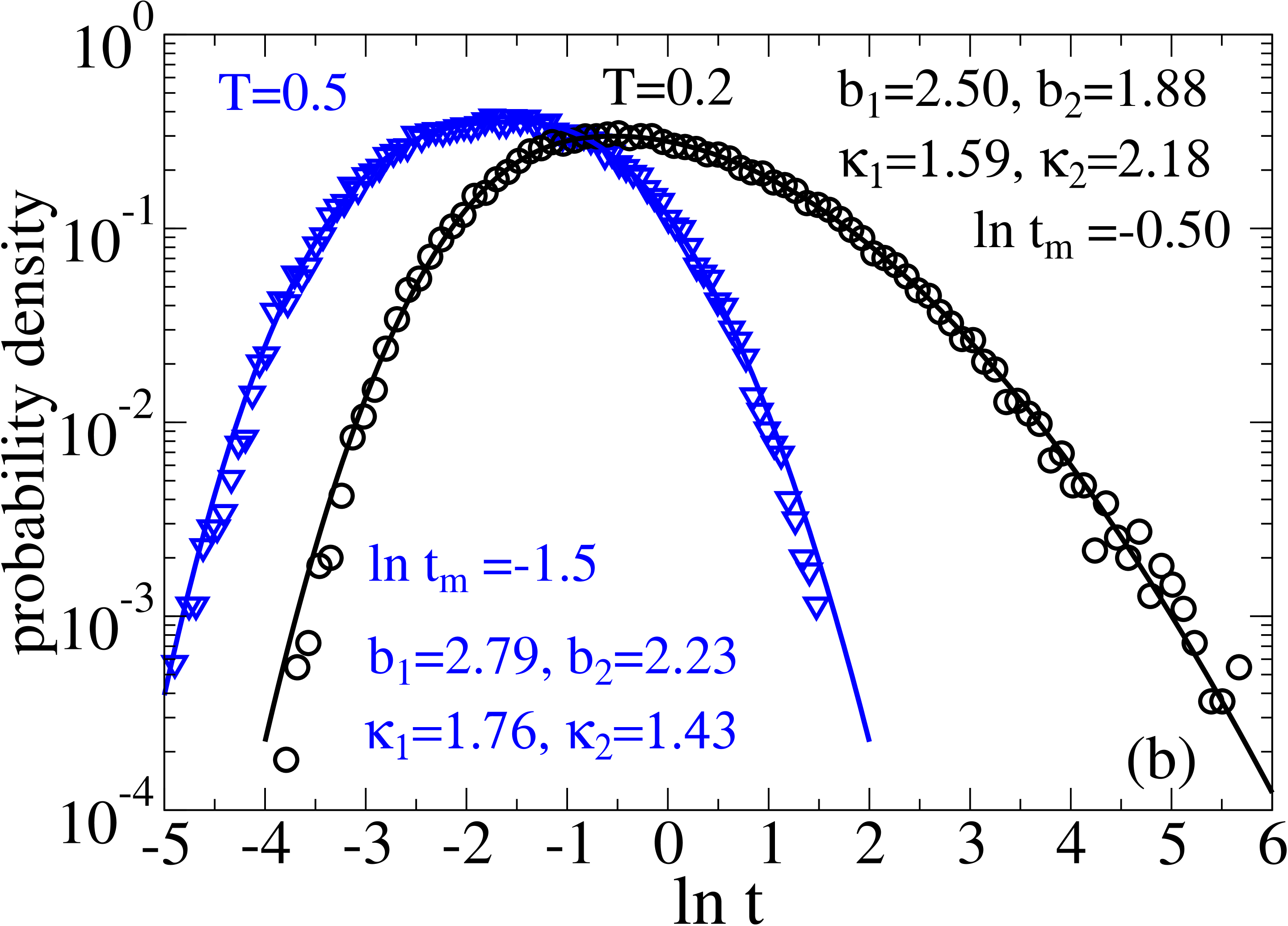
Figure 5: (Color online) Probability density function of log-transformed first escape times, $z=\ln t$, from the interval $[-\lambda,\lambda]$ for two temperatures $T=0.5$ (in blue) and $T=0.2$ (in black). The cases in the different panels are: (a) exponential correlations, (b) power-law correlations with $\gamma=0.8$. The symbols represent simulations data, the lines correspond to a fit with the probability density (17). Parameters are shown in the panels. With decreasing temperature the distributions become broader and the parameter $b_{2}$ smaller. In (c), probability densities of the original non-transformed time variable are plotted which correspond to the part (a). In this case, $\psi(t)$ seems to show some parts with power law dependencies. Especially confusing is the case of $T=0.2$, where the part of distribution with negative exponent $-1.3$ (indicated in red), in a conjunction with $\alpha(t)\approx\alpha_{\rm min}\approx 0.32$ in Fig. 3, a and broad scatter of single trajectory averages in Fig. 4, c can be erroneously interpreted within a CTRW theory with divergent mean residence time.

The success of the scaling argumentation extended from normal to subdiffusive viscoelastic dynamics in stationary Gaussian potentials suggests that the escape time distributions should also be similar. We consider escape of the particles out of $[-\lambda,\lambda]$ spatial interval, which are initially located at its center. The distribution of logarithmically transformed escape times, $z=\ln t$, is plotted in Fig. 5. Indeed, a generalized log-normal distribution of Ref. Goychuk et al. (2017)

$$\psi(t) = \frac{C}{t}\Big{[}e^{-|\ln(t/t_{m})/\kappa_{1}|^{b_{1}}}\theta(t_{m}-t)$$ (17)

$$+e^{-|\ln(t/t_{m})/\kappa_{2}|^{b_{2}}}\theta(t-t_{m})\Big{]},$$

where $C=b_{1}b_{2}/[b_{2}\kappa_{1}\Gamma(1/b_{1})+b_{1}\kappa_{2}\Gamma(1/b_{2})]$ is a normalization constant, $b_{1,2}>1$, and $\kappa_{1,2}>0$, fits excellently to the numerical data for the both considered models of correlations. General features are similar to those of memoryless diffusion. The escape density has a maximum at $\ln t_{m}$ value of the logarithmically transformed time variable. Furthermore, escape in the power-law correlated potentials occurs much faster than in the exponentially correlated potentials. The exponent $b_{2}$ is strongly temperature dependent. With lowering temperature it becomes smaller and closer to one. However, all the moments of RTD remain finite. Notice that this generalized log-normal distribution can sometimes be easily mistaken for a power law, if to plot it in doubly logarithmic coordinates for the original non-transformed time variable as e.g. in Fig. 5, c, in the case of exponential correlations. It is also reminiscent of a stretched exponential distribution Goychuk (2009). This is why to know the moments of experimental distributions is important, as well as using other representations of experimental data, upon a transformation of random variable, like in our Fig. 5, a, b. This would allow a new look on the existing experimental data, such as e.g. in Ref. Wong et al. (2004), in the light of our model. Indeed, it is very tempting to interpret $\psi(t)\propto 1/t^{1.3}$ in Fig. 5, c for $T=0.2$ in conjunction with $\alpha(t)\approx\alpha_{\rm min}\approx 0.32$ in Fig. 3, a, and a strong scatter of single-trajectory averages in Fig. 4, c within the traditional CTRW theory with divergent mean residence time, like done in Ref. Wong et al. (2004). However, real physics in our particular case is very different. In our work, these results are produced by viscoelastic subdiffusion in a random Gaussian potential. Unlike the case of CTRW subdiffusion Metzler et al. (2014), single-trajectory averages have in the studied case of viscoelastic subdiffusion an averaged $\bar{\alpha}$, which correlates well with the power law exponent of the ensemble-average, see in Fig. 4. This can provide an important experimental criterion to distinguish among various theoretical explanations possible.

III.3.1 Digression on dimensionality

The question of whether one can or not directly apply the results obtained within a one-dimensional model to two- or three-dimensional diffusion in living cells, or dense heterogeneous polymeric liquids is not trivial. First of all, in the one-dimensional case the particle cannot avoid a trap, or a barrier on its way. However, in 2d and 3d it can find the ways around. This remark is especially important for viscoelastic subdiffusion, which can thoroughly explore the space. Indeed, the fractal Hausdorff dimension of fBm trajectories occupying 3d space is Feder (1991) $d_{H}=2/\alpha$, for $2/3<\alpha<1$, and $d_{H}=3$, for $0<\alpha<2/3$. Hence, for $\alpha<2/3$ the fBm fills densely the three-dimensional Euclidean space and it can find all possible ways around. Thus, our first expectation is that in 2d and 3d viscoelastic subdiffusion will generally more easily overcome the medium’s disorder than in 1d. At the same time, it will show a significant scatter in single-trajectory averages. This is namely a kind of behavior which is often observed, and which our 1d theory predicts. To reveal the regime of Sinai like diffusion in higher dimensions seems less likely, unless the disorder is very irregular, of singular type, like in the case of exponential correlations. In the extreme case of disorder uncorrelated on the sites of lattice, it is easy to grasp that to avoid the traps is hardly possible beyond the linear sizes of several lattice constants. These preliminary considerations require a lot of further research which is computationally very demanding. Nevertheless, the insights obtained from simplified 1d models are very important. They can drive and strongly impact the follow-up research, as it has been multiply proven in the historical development of the theory of both normal and anomalous diffusion.

IV Summary and conclusions

In this work, we studied numerically viscoelastic subdiffusion governed by a fractional Langevin equation in stationary Gaussian random potentials for several models of decaying correlations. Such theoretical models are of special interest in the context of biologically relevant viscoelastic subdiffusion in random environments. Our study revealed several surprises. First of all, on the ensemble level the influence of random potential is almost completely negligible for $\sigma=k_{B}T$. Viscoelastic subdiffusion easily wins over the potential randomness, even if the potential is wildly fluctuating as in the case of exponentially decaying correlation, see in Fig. 1. This is a very unexpected result because (i) normal diffusion in such potentials is suppressed by the factor $\exp[-(\sigma/k_{B}T)^{2}]$ which is approximately $0.368$ in this case, (ii) slowness combined with sluggishness intuitively should result into a super-slowness. However, this intuition fails completely. Nevertheless, this surprising result was already partially anticipated in view of akin influence of the periodic potentials on viscoelastic subdiffusion Goychuk (2009, 2012a). It has precisely the same explanation: Distributions of the escape times out of metastable minima have finite moments, and the asymptotic behavior is determined by viscoelastic long-time correlations in the medium that yield unobstructed subdiffusion. With the increase of the disorder strength to $\sigma=2k_{B}T$, the presence of a transient behavior becomes slightly visible. However, on the ensemble level the effect is really weak and one can clearly deduce from numerics that the asymptotic regime is almost achieved at the end of our simulations. At odds with $\exp[-(\sigma/k_{B}T)^{2}]\approx 0.018$ for normal diffusion in this case, viscoelastic subdiffusion is practically not suppressed at all. Nevertheless, in spite of a barely noticeable effect on the ensemble level, single-trajectory averages exhibit a substantial scatter. This can provide a key insight to understand some experiments on subdiffusion in biological cells. With a further increase of randomness strength to $\sigma\sim(5-10)k_{B}T$, a very distinct behavior emerges. For $\sigma=10\;k_{B}T$, it is clearly Sinai subdiffusion, $\langle\delta x^{2}(t)\rangle\propto\ln^{4}(t/t_{0})$, for both exponential and power law correlations. Its origin can be explain in a very similar manner as in the case of normal diffusion in such potentials. It is caused by extremal value fluctuations of the potential $\delta U_{\rm max}(x)\propto\sqrt{\ln x}$ and has clearly a transient character. Ultimately, the regime of potential-free viscoelastic subdiffusion will be reached. However, the transients can last so long that they never will be reached in reality. For an intermediate $\sigma=5\;k_{B}T$, a more complex behavior in Eq. (12) substantiate, in agreement with numerics, the reasoning based on a scaling argumentation Goychuk et al. (2017) and Arrhenius character of viscoelastic diffusion over potential barriers Goychuk (2009). It can, however, be also described with some effective power law exponent $\alpha(t)$ that temporally can be nearly a constant, which can be confused with a CTRW subdiffusion Goychuk et al. (2017).

The author is confident that these highly surprising results will attract attention of both theorists and experimentalists leading to a further research in this currently least explored area of anomalous diffusion.

Conflicts of interest

There are various conflicts of interest with competitors in the field of anomalous diffusion and its application to biological systems.

Appendix A Fractional Fokker-Planck dynamics in Gaussian disordered potentials

Let us consider a fractional dynamics governed by the fractional Fokker-Planck equation (FFPE) Metzler et al. (1999); Metzler and Klafter (2000); Goychuk et al. (2006); Heinsalu et al. (2006)

$$\frac{{\partial}^{\alpha}P(x,t)}{{\partial}t^{\alpha}}=D_{\alpha}\frac{\partial}{\partial x}\left(e^{-\beta U(x)}\frac{\partial}{\partial x}\,e^{\beta U(x)}P(x,t)\right)\;\;$$ (18)

for the probability density $P(x,t)$ of particles in a potential $U(x)$. Here, like in Eq. (3), $\partial^{\alpha}P(x,t)/\partial t^{\alpha}$ denotes fractional Caputo time derivative, $\beta=1/(k_{B}T)$ is inverse temperature, and $D_{\alpha}=k_{B}T/\eta_{\alpha}$ is fractional diffusion coefficient, $0<\alpha<1$. It must be emphasized that FFPE (18) is not a probability density counterpart of FLE (3) in the particular case $\eta_{0}=0$, contrary to what was stated e.g. in an important review Zaslavsky (2002). Wrong assertions of this kind are the reason for co-existence of two very different fractional dynamics, both named fractional in the literature despite fundamental differences between them, as it has been clarified later on, see e.g. in Ref. Goychuk and Hänggi (2011). The reader should be warned of this. Fractional dynamics in the transport direction $x$ can result from an extra (infinite) orthogonal dimension, like in the comb model ben Avraham and Havlin (2000), where it leads to $\alpha=1/2$ in the transport direction $x$. We impose a periodic boundary condition, $U(x+L)=U(x)$, with a very large spatial period $L$, which is a standard trick in treating disordered systems Bouchaud and Georges (1990). In the case of diffusion of regulatory proteins on a circular bacterial DNA it is even natural. By applying in addition a constant biasing force $f_{0}$, $U(x)\to V(x)=U(x)-f_{0}x$ it has been shown in Ref. Goychuk et al. (2006); Heinsalu et al. (2006), that the mean displacement of particles follows $\langle\delta x(t)\rangle=\bar{v}(f_{0})t^{\alpha}/\Gamma(1+\alpha)$, with mean subvelocity

$$\bar{v}_{\alpha}(f_{0})=\frac{D_{\alpha}L\,[1-\exp(-\beta f_{0}L)]}{\int_{0}^{L}\mathrm{d}x\int_{x}^{x+L}\mathrm{d}y\,\exp(-\beta[V(x)-V(y)])},\,$$ (19)

which generalizes a famous result by Stratonovich Stratonovich (1958, 1967); Risken (1989) towards FFPE dynamics in arbitrary periodic potentials. The corresponding biased diffusion obeys a universal scaling relation Goychuk et al. (2006); Heinsalu et al. (2006)

$$\lim_{t\to\infty}\frac{\langle\delta x^{2}(t)\rangle}{\langle\delta x(t)\rangle^{2}}=\frac{2\Gamma^{2}(\alpha+1)}{\Gamma(2\alpha+1)}-1\;,$$ (20)

reflecting stochastic properties of underlying random clock governing this type of fractional subdiffusion Goychuk and Hänggi (2011). The unbiased subdiffusion, $f_{0}\to 0$, obeys $\langle\delta x^{2}(t)\rangle_{f_{0}=0}=2\bar{D}_{\alpha}t^{\alpha}/\Gamma(1+\alpha)$, with a potential-renormalized anomalous diffusion coefficient Heinsalu et al. (2007b); Goychuk and Hänggi (2011),

$$\bar{D}_{\alpha}=\frac{\,D_{\alpha}L^{2}}{\int_{0}^{L}\mathrm{d}x\,\exp\left[\beta U(x)\right]\int_{0}^{L}\mathrm{d}y\,\exp\left[-\beta U(y)\right]},\,$$ (21)

which follows from (19) upon use of the fluctuation-dissipation theorem, or linear response relation, $\bar{D}_{\alpha}=\lim_{f_{0}\to 0}k_{B}T\bar{v}_{\alpha}(f_{0})/f_{0}$. It generalizes a celebrated result by Lifson and Jackson Lifson and Jackson (1962) towards fractional FFPE diffusion in periodic potentials. The results in Eqs. (19)-(21) were verified in extensive numerical simulations for various periodic potentials Goychuk et al. (2006); Heinsalu et al. (2006, 2007b) and are firmly established. Using a spatial average, $\overline{C_{L}^{\pm}}=(1/L)\int_{0}^{L}w_{\pm}(x)dx$, of statistical weight-functions $w_{\pm}=\exp[\pm\beta U(x)]$, the result in (21) can be rewritten as $\bar{D}_{\alpha}=D_{\alpha}/[\overline{C_{L}^{+}}\;\overline{C_{L}^{-}}]$. Furthermore, assuming ergodicity of the random process $w_{\pm}(x)$ in space, one can replace in the limit $L\to\infty$ the spatial averages with the corresponding ensemble averages and for Gaussian disorder we obtain the central result of this Appendix:

$$\langle\delta x^{2}(t)\rangle=2D_{\alpha}e^{-\sigma^{2}/(k_{B}T)^{2}}t^{\alpha}/\Gamma(1+\alpha).$$ (22)

Following Goychuk and Kharchenko (2014) it is easy to show that this result is valid asymptotically for any stationary Gaussian potential with decaying correlations. This result generalizes the normal-diffusion result by Zwanzig Zwanzig (1988) et al. towards FFPE subdiffusion in such potentials. However, it is not applicable to viscoelastic fractional subdiffusion studied in this paper.

Appendix B Velocity autocorrelation function for nanoparticles in viscoeleastic media and neglection of inertial effects

In this Appendix, a justification of the neglection of inertial effects is given. For free viscoelastic subdiffusion with the inertial effects included, the normalized stationary velocity autocorrelation function (VACF) in the Laplace space reads, see Eq. (B26) in Ref. Goychuk (2012a) or Eq. (A3) in Ref. Goychuk (2009),

$$\tilde{K}_{v}(s)=\frac{1}{s+\tilde{\eta}(s)/m},$$ (23)

where $\tilde{\eta}(s)$ is Laplace-transform of a general memory kernel and $m$ is the mass of particles. For the memory kernel in this paper it is

$$\tilde{K}_{v}(s)=\frac{1}{s+\gamma_{0}+\gamma_{\alpha}s^{\alpha-1}}\;,$$ (24)

where $\gamma_{0}=\eta_{0}/m$ and $\gamma_{\alpha}=\eta_{\alpha}/m$. In this case, $\int_{0}^{\infty}K_{v}(t)dt=0$, for any $\eta_{\alpha}\neq 0$. For normal diffusion with $\eta_{\alpha}=0$, $K_{v}(t)=\exp(-t/\tau_{v}^{(0)})$, in the time domain, where $\tau_{v}^{(0)}=m/\eta_{0}$ the velocity relaxation constant. For the case of purely fractional friction with $\eta_{0}=0$, $K_{v}(t)=E_{2-\alpha}[-(t/\tau_{v})^{2-\alpha}]$ Goychuk (2012a); Lutz (2001), where $E_{a}(z)=E_{a,b=1}(z)$ is the Mittag-Leffler function, and $\tau_{v}=(m/\eta_{\alpha})^{1/(2-\alpha)}$ is the velocity relaxation constant of anomalous relaxation, which has in this case a negative power-law tail, $K_{v}(t)\propto-1/(t/\tau_{v})^{2-\alpha}$, for $t\gg\tau_{v}$. Notice, that in both cases the velocity relaxation is instant in the strict limit $m\to 0$. This limit is singular because the mean-square thermal velocity diverges $v_{T}^{2}=k_{B}T/m\to\infty$. This the reason why both the normal Brownian motion (Wiener process) and fBm are not differentiable, being singular processes in this respect, though of a wide and common use in physics. Furthermore, after some lengthy algebra one obtains the following exact result in the case $\alpha=1/2$:

$$K_{v}(t)=\sum_{i=1}^{3}c_{i}z_{i}^{2}\exp(z_{i}^{2}t/\tau_{v}){\rm erfc}(z_{i}\sqrt{t/\tau_{v}})$$ (25)

where $\tau_{v}=(m/\eta_{\alpha})^{2/3}$,

$$z_{1} = \frac{2}{3\cdot 4^{1/3}}\frac{\gamma_{0}\tau_{v}}{(\sqrt{1+12(\gamma_{0}\tau_{v})^{3}/81}-1)^{1/3}}$$ (26)

$$- \frac{4^{1/3}}{2}(\sqrt{1+12(\gamma_{0}\tau_{v})^{3}/81}-1)^{1/3},$$

$$z_{2,3} = -z_{1}/2\pm i\frac{\sqrt{3}}{2}$$ (27)

$$\times \Big{[}\frac{4^{1/3}}{2}(\sqrt{1+12(\gamma_{0}\tau_{v})^{3}/81}-1)^{1/3}$$

$$+ \frac{2}{3\cdot 4^{1/3}}\frac{\gamma_{0}\tau_{v}}{(\sqrt{1+12(\gamma_{0}\tau_{v})^{3}/81}-1)^{1/3}}\Big{]}$$

and

$$c_{1} = \frac{1}{(z_{1}-z_{2})(z_{1}-z_{3})},$$

$$c_{2} = \frac{1}{(z_{1}-z_{2})(z_{3}-z_{2})},$$

$$c_{3} = \frac{1}{(z_{2}-z_{3})(z_{1}-z_{3})}\;.$$ (28)

For $\gamma_{0}=0$, $z_{1}=1$ and $z_{2,3}=-1/2\pm i\sqrt{3}/2$. Independently of $\gamma_{0}$, the asymptotics reads

$$K_{v}(t)\sim-\frac{1}{2\sqrt{\pi}(t/\tau_{v})^{3/2}}$$ (29)

for $t\gg\tau_{v}$. Notice that already for $t>100\tau_{v}$, $K_{v}(t)$ is really small and the overdamped approximation can be accurately used, on theoretical grounds. In fact, however, the initial ballistic regime is already over for $t>(3-5)\tau_{v}$ in reality, see e. g. Figs. 5, 6 in Ref. Goychuk (2012a). It is important to emphasize that this fact does not contradict to another fact that double integration of $v_{T}^{2}K_{v}(t)$ yields the mean square displacement whose behavior is determined by the discussed tail and where the time scale $\tau_{v}$ drops out. This important time scale defines the initial ballistic regime, see in Refs. Goychuk (2009, 2012a) which is of no importance in this work. For $0\leq\gamma_{0}\tau_{v}<\gamma_{0}^{(c)}\tau_{v}\approx 0.220404$, $K_{v}(t)$ changes its sign precisely three times. For a larger $\gamma_{0}\tau_{v}$, a single change of the sign occurs.

Let us estimate now the time scale $\tau_{v}$ of the velocity relaxation for diffusion of nanoparticles in viscoelastic cytosol of living cells. For the colloidal gold particles with radius $R=2.5$ nm in Ref. Guigas et al. (2007) subdiffusion was found in HeLa cells with $\alpha\approx 0.51\approx 0.5$ and $D_{\alpha}\approx 0.644\;{\rm\mu m^{2}/s^{\alpha}}$ (see in Table I in Ref. Goychuk (2012b)) on the time scale up to 1 s, at least. Let us use this experimental value and the generalized Einstein relation $D_{\alpha}=k_{B}T/\eta_{\alpha}$ to estimate $\tau_{v}=\left(4\pi\rho R^{3}D_{1/2}/(3k_{B}T)\right)^{2/3}$, where $\rho$ is the mass density of particle. With the gold mass density $\rho=19.3$ kg/m³ and room $k_{B}T=4.1{\rm\;pN\cdot nm}$, we obtain $\tau_{v}\approx 28.08$ ps (picoseconds!). For lighter particles such as globular proteins with $\rho\sim 1.2$ kg/m³ it will be even smaller. Thus, already on the time scale of nanoseconds and larger the inertial effects are completely negligible, for sure. Furthermore, the normal diffusion coefficient $D_{0}$ in the water component of cytosol can be estimated using the Einstein-Stokes relation as $D_{0}=k_{B}T/(6\pi\zeta_{w}R)$, where $\zeta_{w}\approx 1\;{\rm mPa\cdot s}$ is water viscosity. This yields $D_{0}\approx 87\;{\rm\mu m^{2}/s}$. The corresponding time $\tau_{0}$ separating the initially normal diffusion and subdiffusion in our paper is hence $\tau_{0}=(D_{1/2}/D_{0})^{2}\approx 54.77\;\mu$s. It is of the order $10^{6}$ larger than $\tau_{v}$, which once again confirms that the inertial effects are completely negligible. In fact, the time step in our numerical simulations exceeds this estimated $\tau_{v}$ by orders of magnitude. Furthermore, the scaling time $\tau_{r}$ used in simulations can be expressed for $\alpha=1/2$ via dimensionless $\tilde{\eta}_{0}$ as $\tau_{r}=\tau_{0}/\tilde{\eta}_{0}^{2}$, which for $\tilde{\eta}_{0}=0.1$ used in numerics gives $\tau_{r}=100\tau_{0}\approx 5.48$ ms. Hence, the maximal time $t_{\rm max}=2\times 10^{5}$ in our numerics corresponds to about $t_{\rm max}=1096$ s. The corresponding length scale, which we took to be the correlation scale, is estimated as $\lambda=\tau_{r}^{1/4}(D_{1/2}\sigma/k_{B}T)^{1/2}\approx 0.218\sqrt{\sigma/k_{B}T}$ $\mu$m, i.e. $\lambda\approx 0.308$ $\mu$m for $\sigma=2$ (in units of $k_{B}T$), or $\lambda\approx 0.689$ $\mu$m for $\sigma=10$, which are typical mesh sizes in random actin meshworks Wong et al. (2004).

B.1 Overdamped approximation in a potential

Also for dynamics in random potentials one can show that the overdamped approximation works typically well for colloidal particles in viscoelastic fluids. Random potentials considered in this paper are locally piece-wise parabolic. Therefore, it compels to consider relaxation in a parabolic potential with curvature $\kappa$. The corresponding position relaxation function, which coincides with normalized stationary autocorrelation function of the coordinate Goychuk (2012a), for the model considered reads,

$$\tilde{\theta}(s)=\frac{s+\gamma_{0}+\gamma_{\alpha}s^{\alpha-1}}{s^{2}+\gamma_{0}s+\gamma_{\alpha}s^{\alpha}+\omega_{0}^{2}}\;,$$ (30)

in the Laplace-space, cf. Eq. (B7) in Ref. Goychuk (2012a). Here, $\omega_{0}=\sqrt{\kappa/m}$ is vibrational frequency. To clarify whether relaxation dynamics is overdamped or not it is convenient to scale time in the units of $1/\omega_{0}$, and $s\to\tilde{s}=s/\omega_{0}$. Then, the correspondingly scaled, relevant non-dimensional frictional constants read, $\bar{\gamma}_{0}=\gamma_{0}/\omega_{0}$, and $\bar{\gamma}_{\alpha}=1/(\omega_{0}\tau_{v})^{2-\alpha}$, where $\tau_{v}$ is the above time constant of a potential-free anomalous relaxation of velocity. It is absolutely clear that the dynamics is overdamped for $\bar{\gamma}_{0}>2$ when $\bar{\gamma}_{\alpha}=0$. It is also beyond doubts that it will be overdamped for a smaller value of $\bar{\gamma}_{0}$ in the case when an additional memory friction is present, especially if it is overdamped already for $\gamma_{0}=0$ due to the memory friction alone. Hence, let us first estimate $\gamma_{0}$. For a gold sphere of radius $2.5$ nm in water we have: $\eta_{0}\approx 4.713\cdot 10^{-11}$ kg/s, and $m\approx 1.263\cdot 10^{-24}$ kg. Hence, $\gamma_{0}\approx 3.731\cdot 10^{13}$ 1/s. Therefore, for any frequency $\omega_{0}$ lower that $10^{13}$ 1/s, or about $300$ cm^-1 in spectroscopic units, which is a typical frequency of molecular vibrations, the dynamics of such a colloidal particle in a trapping potential is clearly overdamped. Let us estimate this frequency in a worse case scenario of a singular disorder corresponding to exponentially decaying correlations in space. The disorder is regularized by considering it on a lattice with the grid constant $\Delta x$ Goychuk and Kharchenko (2014); Goychuk et al. (2017). We can estimate a typical value of $\kappa$ from the condition $\langle\delta f^{2}(0)\rangle^{1/2}\sim\kappa\Delta x$, where $\langle\delta f^{2}(0)\rangle^{1/2}=\sqrt{2}\sigma/\sqrt{\Delta x\lambda}$ is the rms amplitude of the random force fluctuations Goychuk et al. (2017). This yields an estimate $\kappa\sim 2^{1/2}\sigma/[(\Delta x)^{3/2}\lambda^{1/2}]$. With $\lambda=308$ nm and $\Delta x=0.02\lambda=6.16$ nm, for $\sigma=2\;k_{B}T_{r}=8.2\;{\rm pN\cdot nm}$, we have $\kappa\approx 0.0432$ pN/nm, which for $m=1.263\cdot 10^{-24}$ kg yields $\omega_{0}=\sqrt{\kappa/m}\sim 5.85\cdot 10^{9}$ 1/s. The corresponding $\bar{\gamma}_{0}\approx 6377.8$ is really large. Let us estimate also $\bar{\gamma}_{\alpha}$ in this case. With $\tau_{v}=28.08$ ps (see above) we obtain $\bar{\gamma}_{\alpha}\approx 15.02$. For such a large $\bar{\gamma}_{\alpha}$, dynamics is clearly overdamped even for $\bar{\gamma}_{0}=0$. Indeed, the case with $\gamma_{0}=0$ for arbitrary $\alpha$ was studied in Refs. Burov and Barkai (2008a, b). It has been shown therein that for $\alpha=1/2$, the relaxation is overdamped and monotonous at $\omega_{0}<\omega_{m}=0.426$ in the units where $\tau_{v}=1$. This critical condition translates into $\bar{\gamma}_{\alpha}>\gamma_{m}=3.596$, in our notations. Clearly, inertial effects are completely negligible from all points of view. Indeed, motion of colloidal particles can be treated typically as overdamped already due to the water component of such complex viscoelastic media as polymeric solutions and cytosol. In the case of power law potential correlations, subdiffusion will be overdamped for a much wider range of parameters. Indeed, in this case a typical $\kappa\sim 2\sigma/\lambda^{2}$ is much smaller than in the case of singular disorder. This indicates that overdamped approximation can be justified in many cases and it presents an important model of general interest.

Appendix C Numerical algorithm

Numerical algorithm to propagate the stochastic dynamics in Eq. (8a), (8b) is based on the well-known stochastic Heun algorithm, or the second order stochastic Runge-Kutta method Gard (1988). Below we sketch it. First, we rewrite (8a), (8b) as

$$\dot{x}=F(x,x_{i})+\sqrt{2D_{0}}\zeta_{0}(t),$$

$$\dot{x}_{i}=\nu_{i}(x-x_{i})+\sqrt{2D_{i}}\zeta_{i}(t),$$ (31)

with $D_{0}=k_{B}T/\eta_{0}$, $D_{i}=k_{B}T/\eta_{i}$, and $F(x,x_{i})=[f(x)-\sum_{i=1}^{N}k_{i}(x-x_{i})]/\eta_{0}$. On each integration time step $\Delta t$ one generates anew $N+1$ independent zero-mean Gaussian variables $W_{i}$ with unit variance, $i=0,1,2...N$ (Mersenne Twister pseudo-random number generator was used for this). Each propagation step in the discretized time dynamics, $x_{k}=x(k\Delta t)$, $x_{i,k}=x_{i}(k\Delta t)$, from $t_{k}=k\Delta t$ to $t_{k+1}=t_{k}+\Delta t$ consists of two substeps. In the first substep,

$$x_{k}^{(1)}=x_{k}+F(x_{k},x_{i,k})\Delta t+\sqrt{2D_{0}\Delta t}W_{0},$$

$$x_{i,k}^{(1)}=x_{i,k}+\nu_{i}(x_{k}-x_{i,k})\Delta t+\sqrt{2D_{i}\Delta t}W_{i}\;.$$ (32)

In the second (final) step,

$$x_{k+1} = x_{k}+\left[F(x_{k},x_{i,k})+F(x_{k}^{(1)},x_{i,k}^{(1)})\right]\Delta t/2$$ (33)

$$+ \sqrt{2D_{0}\Delta t}W_{0},$$

$$x_{i,k+1} = x_{i,k}+\nu_{i}\left[x_{k}+x_{k}^{(1)}-x_{i,k}-x_{i,k}^{(1)})\right]\Delta t/2$$

$$+ \sqrt{2D_{i}\Delta t}W_{i}\;.$$

Notice that $W_{i}$ must be the same numbers on the both substeps Gard (1988). The algorithm was implemented in CUDA and propagated in parallel (many different particles with different initially random preparations at the same time) on GPU processors.

References

- Shlesinger (1974) M. F. Shlesinger, Asymptotic solutions of continuous-time random walks, J. Stat. Phys. 10, 421 (1974).
- Scher and Montroll (1975) H. Scher and E. W. Montroll, Anomalous transit-time dispersion in amorphous solids, Phys. Rev. B 12, 2455 (1975).
- Bouchaud and Georges (1990) J.-P. Bouchaud and A. Georges, Anomalous diffusion in disordered media: Statistical mechanisms, models and physical applications, Phys. Rep. 195, 127 (1990).
- ben Avraham and Havlin (2000) D. ben Avraham and S. Havlin, Diffusion and Reactions in Fractals and Disordered Systems (Cambridge University Press, Cambridge, 2000).
- Hughes (1995) B. D. Hughes, Random Walks and Random Environments (Clarendon Press, Oxford, 1995).
- Bouchaud et al. (1990) J. Bouchaud, A. Comtet, A. Georges, and P. L. Doussal, Classical diffusion of a particle in a one- dimensional random force field, Ann. Phys. (N.Y.) 201, 285 (1990).
- Bouchaud (1992) J. P. Bouchaud, Weak ergodicity breaking and aging in disordered systems, J. Phys. I (Paris) 2, 1705 (1992).
- Metzler and Klafter (2000) R. Metzler and J. Klafter, The random walk’s guide to anomalous diffusion: a fractional dynamics approach, Phys. Rep. 339, 1 (2000).
- Klafter et al. (2011) J. Klafter, S. C. Lim, and R. Metzler, eds., Fractional Dynamics: Recent Advances (World Scientific, New Jersey, 2011).
- Goychuk (2012a) I. Goychuk, Viscoelastic Subdiffusion: Generalized Langevin Equation Approach, Adv. Chem. Phys. 50, 187 (2012a).
- Metzler et al. (2014) R. Metzler, J.-H. Jeon, A. G. Cherstvy, and E. Barkai, Anomalous diffusion models and their properties: non-stationarity, non-ergodicity, and ageing at the centenary of single particle tracking, Phys. Chem. Chem. Phys. 16, 24128 (2014).
- Mason and Weitz (1995) T. G. Mason and D. A. Weitz, Optical Measurements of Frequency-Dependent Linear Viscoelastic Moduli of Complex Fluids, Phys. Rev. Lett. 74, 1250 (1995).
- Amblard et al. (1996) F. Amblard, A. C. Maggs, B. Yurke, A. N. Pargellis, and S. Leibler, Subdiffusion and Anomalous Local Viscoelasticity in Actin Networks, Phys. Rev. Lett. 77, 4470 (1996).
- Saxton and Jacobsen (1997) M. J. Saxton and K. Jacobsen, Single-particle tracking: application to membrane dynamics, Ann. Rev. Biophys. Biomolec. Struc. 26, 373 (1997).
- Waigh (2005) T. A. Waigh, Microrheology of complex fluids, Rep. Progr. Phys. 68, 685 (2005).
- Seisenberger et al. (2001) G. Seisenberger, M. U. Ried, T. Endress, H. Büning, M. Hallek, and C. Bräuchle, Real-time single-molecule imaging of the infection pathway of an adeno-associated virus, Science 294, 1929 (2001).
- Caspi et al. (2002) A. Caspi, R. Granek, and M. Elbaum, Diffusion and directed motion in cellular transport, Phys. Rev. E 66, 011916 (2002).
- Weiss et al. (2004) M. Weiss, M. Elsner, F. Kartberg, and T. Nilsson, Anomalous Subdiffusion Is a Measure for Cytoplasmic Crowding in Living Cells, Biophys. J. 87, 3518 (2004).
- Tolic-Norrelykke et al. (2004) I. M. Tolic-Norrelykke, E.-L. Munteanu, G. Thon, L. Oddershede, and K. Berg-Sorensen, Anomalous diffusion in living yeast cells, Phys. Rev. Lett. 93, 078102 (2004).
- Banks and Fradin (2005) D. S. Banks and C. Fradin, Anomalous Diffusion of Proteins Due to Molecular Crowding, Biophys. J. 89, 2960 (2005).
- Barkai et al. (2012) E. Barkai, Y. Garini, and R. Metzler, Strange kinetics of single molecules in living cells, Phys. Today 65 (8), 29 (2012).
- Bruno et al. (2011) L. Bruno, M. Salierno, D. E. Wetzler, M. A. Desposito, and V. Levi, Mechanical properties of organelles driven by microtubuli-dependent molecular motors in living cells, PLoS ONE 6, e18332 (2011).
- Bruno et al. (2009) L. Bruno, V. Levi, M. Brunstein, and M. A. Desposito, Transition to superdiffusive behavior in intracellular actin-based transport mediated by molecular motors, Phys. Rev. E 80, 011912 (2009).
- Golding and Cox (2006) I. Golding and E. C. Cox, Physical nature of bacterial cytoplasm, Phys. Rev. Lett. 96, 098102 (2006).
- Guigas et al. (2007) G. Guigas, C. Kalla, and M. Weiss, Probing the nanoscale viscoelasticity of intracellular fluids in living cells, Biophys. J. 93, 316 (2007).
- Szymanski and Weiss (2009) J. Szymanski and M. Weiss, Elucidating the Origin of Anomalous Diffusion in Crowded Fluids, Phys. Rev. Lett. 103, 038102 (2009).
- Höfling and Franosch (2013) F. Höfling and T. Franosch, Anomalous transport in the crowded world of biological cells, Rep. Prog. Phys. 76, 046602 (2013).
- Jeon et al. (2011) J. H. Jeon, V. Tejedor, S. Burov, E. Barkai, C. Selhuber-Unkel, K. Berg-Sørensen, L. Oddershede, and R. Metzler, In vivo anomalous diffusion and weak ergodicity breaking of lipid granules, Phys. Rev. Lett. 106, 048103 (2011).
- Luby-Phelps (2013) K. Luby-Phelps, The physical chemistry of cytoplasm and its influence on cell function: an update, Mol. Biol. Cell 24, 2593 (2013).
- Pan et al. (2009) W. Pan, L. Filobelo, N. D. Q. Pham, O. Galkin, V. V. Uzunova, and P. G. Vekilov, Viscoelasticity in Homogeneous Protein Solutions, Phys. Rev. Lett. 102, 058101 (2009).
- Wong et al. (2004) I. Y. Wong, M. L. Gardel, D. R. Reichman, E. R. Weeks, M. T. Valentine, A. R. Bausch, and D. A. Weitz, Anomalous Diffusion Probes Microstructure Dynamics of Entangled F-Actin Networks, Phys. Rev. Lett. 92, 178101 (2004).
- Harrison et al. (2013) A. W. Harrison, D. A. Kenwright, T. A. Waigh, P. G. Woodman, and V. J. Allan, Modes of correlated angular motion in live cells across three distinct time scales, Phys. Biol. 10, 036002 (2013).
- Parry et al. (2014) B. R. Parry, I. V. Surovtsev, M. T. Cabeen, C. S. O’Hern, E. R. Dufresne, and C. Jacobs-Wagner, The bacterial cytoplasm has glass-like properties and is fluidized by metabolic activity, Cell 156, 183 (2014).
- Robert et al. (2010) D. Robert, T.-H. Nguyen, F. Gallet, and C. Wilhelm, Diffusion and directed motion in cellular transport, PLoS ONE 4, e10046 (2010).
- Goychuk et al. (2014a) I. Goychuk, V. O. Kharchenko, and R. Metzler, How Molecular Motors Work in the Crowded Environment of Living Cells: Coexistence and Efficiency of Normal and Anomalous Transport, PLoS ONE 9, e91700 (2014a).
- Goychuk et al. (2014b) I. Goychuk, V. O. Kharchenko, and R. Metzler, Molecular motors pulling cargos in the viscoelastic cytosol: how power strokes beat subdiffusion, Phys. Chem. Chem. Phys. 16, 16524 (2014b).
- Goychuk (2015a) I. Goychuk, Anomalous transport of subdiffusing cargos by single kinesin motors: the role of mechanochemical coupling and anharmonicity of tether, Phys. Biol. 12, 016013 (2015a).
- Tabei et al. (2013) S. M. A. Tabei, S. Burov, H. Y. Kima, A. Kuznetsov, T. Huynha, J. Jureller, L. H. Philipson, A. R. Dinner, and N. F. Scherer, Intracellular transport of insulin granules is a subordinated random walk, Proc. Natl. Acad. Sci. (USA) 110, 4911 (2013).
- Weigel et al. (2011) A. V. Weigel, B. Simon, M. M. Tamkun, and D. Krapf, Ergodic and nonergodic processes coexist in the plasma membrane as observed by single-molecule tracking, Proc. Natl. Acad. Sci. (USA) 108, 6438 (2011).
- Weiss (2013) M. Weiss, Single-particle tracking data reveal anticorrelated fractional Brownian motion in crowded fluids, Phys. Rev. E 88, 010101 (2013).
- Santamaria-Holek et al. (2007) I. Santamaria-Holek, J. M. Rubi, and A. Gadomski, Thermokinetic Approach of Single Particles and Clusters Involving Anomalous Diffusion under Viscoelastic Response, J. Phys. Chem. B 111, 2293 (2007).
- Bertseva et al. (2012) E. Bertseva, D. Grebenkov, P. Schmidhauser, S. Gribkova, S. Jeney, and L. Forro, Optical trapping microrheology in cultured human cells, Eur. Phys. J. E 35, 63 (2012).
- Evers et al. (2013) F. Evers, R. D. L. Hanes, C. Zunke, R. F. Capellmann, J. Bewerunge, C. Dalle-Ferrier, M. C. Jenkins, I. Ladadwa, A. Heuer, R. Castaneda-Priego, and S. U. Egelhaaf, Colloids in light fields: particle dynamics in random and periodic energy landscapes, Eur. Phys. J. Spec. Top. 222, 2995 (2013).
- Hanes et al. (2013) R. D. L. Hanes, M. Schmiedeberg, and S. U. Egelhaaf, Brownian particles on rough substrates: relation between intermediate subdiffusion and asymptotic long-time diffusion, Phys. Rev. E 88, 062133 (2013).
- Nunomura et al. (2006) S. Nunomura, D. Samsonov, S. Zhdanov, and G. Morfill, Self-Diffusion in a Liquid Complex Plasma, Phys. Rev. Lett. 96, 015003 (2006).
- Schubert et al. (2013) M. Schubert, E. Preis, J. C. Blakesley, P. Pingel, U. Scherf, and D. Neher, Mobility relaxation and electron trapping in a donor/acceptor copolymer, Phys. Rev. B 87, 024203 (2013).
- Yang et al. (2003) H. Yang, G. Luo, P. Karnchanaphanurach, T.-M. Louie, I. Rech, S. Cova, L. Xun, and X. S. Xie, Protein Conformational Dynamics Probed by Single-Molecule Electron Transfer, Science 302, 262 (2003).
- Kou and Xie (2004) S. C. Kou and X. S. Xie, Generalized Langevin Equation with Fractional Gaussian Noise: Subdiffusion within a Single Protein Molecule, Phys. Rev. Lett. 93, 180603 (2004).
- Goychuk and Hänggi (2004) I. Goychuk and P. Hänggi, Fractional diffusion modeling of ion channel gating, Phys. Rev. E 70, 051915 (2004).
- Kneller and Hinsen (2004) G. R. Kneller and K. Hinsen, Fractional Brownian dynamics in proteins, J. Chem. Phys. 121, 10278 (2004).
- Min et al. (2005) W. Min, G. Luo, B. J. Cherayil, S. C. Kou, and X. S. Xie, Observation of a Power-Law Memory Kernel for Fluctuations within a Single Protein Molecule, Phys. Rev. Lett. 94, 198302 (2005).
- Calandrini et al. (2010) V. Calandrini, D. Abergel, and G. R. Kneller, Fractional protein dynamics seen by nuclear magnetic resonance spectroscopy: Relating molecular dynamics simulation and experiment, J. Chem. Phys. 133, 145101 (2010).
- Calligari et al. (2011) P. A. Calligari, V. Calandrini, G. R. Kneller, and D. Abergel, From NMR Relaxation to Fractional Brownian Dynamics in Proteins: Results from a Virtual Experiment, J. Phys. Chem. B 115, 12370 (2011).
- Calligari et al. (2015) P. A. Calligari, V. Calandrini, J. Ollivier, J.-B. Artero, M. Härtlein, M. Johnson, and G. R. Kneller, Adaptation of Extremophilic Proteins with Temperature and Pressure: Evidence from Initiation Factor 6, J. Phys. Chem. B 119, 7860 (2015).
- Goychuk (2015b) I. Goychuk, Modeling magnetosensitive ion channels in the viscoelastic environment of living cells, Phys. Rev. E 92, 042711 (2015b).
- Hu et al. (2016) X. Hu, L. Hong, M. D. Smith, T. Neusius, X. Cheng, and J. C. Smith, The dynamics of single protein molecules is non-equilibrium and self-similar over thirteen decades in time, Nat. Phys. 12, 171 (2016).
- Kneller et al. (2011) G. R. Kneller, K. Baczynski, and M. Pasenkiewicz-Gierula, Communication: Consistent picture of lateral subdiffusion in lipid bilayers: Molecular dynamics simulation and exact results, J. Chem. Phys. 135, 141105 (2011).
- Jeon et al. (2012) J.-H. Jeon, H. M.-S. Monne, M. Javanainen, and R. Metzler, Anomalous Diffusion of Phospholipids and Cholesterols in a Lipid Bilayer and its Origins, Phys. Rev. Lett. 109, 188103 (2012).
- Jeon et al. (2016) J.-H. Jeon, M. Javanainen, H. Martinez-Seara, R. Metzler, and I. Vattulainen, Protein Crowding in Lipid Bilayers Gives Rise to Non-Gaussian Anomalous Lateral Diffusion of Phospholipids and Proteins, Phys. Rev. X 6, 021006 (2016).
- Kong et al. (2016) M. Kong, L. Liu, X. Chen, K. I. Driscoll, P. Mao, S. Böhm, N. M. Kad, S. C. Watkins, K. A. Bernstein, J. J. Wyrick, J.-H. Min, and B. V. Houten, Single-molecule imaging reveals that Rad4 (XPC) employs a dynamic DNA damage recognition process, Mol. Cel. 64, 376 (2016).
- Kong and Houten (2017) M. Kong and B. V. Houten, Rad4 recognition-at-a-distance: Physical basis of conformation- specific anomalous diffusion of DNA repair proteins, Prog.Biophys. Mol. Biolog. 127, 93 (2017).
- Liu et al. (2017) L. Liu, M. Kong, N. R. Gassman, B. D. Freudentha, R. Prasad, S. Zhen, S. C. Watkins, S. H. Wilson, and B. V. Houten, PARP1 changes from three-dimensional DNA damage searching to one-dimensional diffusion after auto-PARylation or in the presence of APE1, Nucl. Acid. Res. 45, 12834 (2017).
- Sinai (1982) Y. G. Sinai, The limiting behavior of a one-dimensional random walk in random medium, Theor. Prob. Appl. 27, 247 (1982).
- Goychuk and Hänggi (2011) I. Goychuk and P. Hänggi, in Fractional Dynamics: Recent Advances, edited by J. Klafter, S. C. Lim, and R. Metzler (World Scientific, New Jersey, 2011) Chap. 13, pp. 305–327.
- Weiss (1999) U. Weiss, Quantum Dissipative Systems, 2nd ed. (World Scientific, Singapore, 1999).
- Pottier (2003) N. Pottier, Aging properties of an anomalously diffusing particle, Physica A 317, 371 (2003).
- Kupferman (2004) R. Kupferman, Fractional Kinetics in Kac-Zwanzig Heat Bath Models, J. Stat. Phys. 114, 291 (2004).
- Goychuk (2009) I. Goychuk, Viscoelastic subdiffusion: from anomalous to normal, Phys. Rev. E 80, 046125 (2009).
- Goychuk et al. (2006) I. Goychuk, E. Heinsalu, M. Patriarca, G. Schmid, and P. Hänggi, Current and universal scaling in anomalous transport, Phys. Rev. E 73, 020101 (R) (2006).
- Heinsalu et al. (2006) E. Heinsalu, M. Patriarca, I. Goychuk, G. Schmid, and P. Hänggi, Fractional Fokker-Planck dynamics: Numerical algorithm and simulations, Phys. Rev. E 73, 046133 (2006).
- Barbi et al. (2005) F. Barbi, M. Bologna, and P. Grigolini, Linear Response to Perturbation of Nonexponential Renewal Processes, Phys. Rev. Lett. 95, 220601 (2005).
- Sokolov and Klafter (2006) I. M. Sokolov and J. Klafter, Field-Induced Dispersion in Subdiffusion, Phys. Rev. Lett. 97, 140602 (2006).
- Heinsalu et al. (2007a) E. Heinsalu, M. Patriarca, I. Goychuk, and P. Hänggi, Use and Abuse of a Fractional Fokker-Planck Dynamics for Time-Dependent Driving, Phys. Rev. Lett. 99, 120602 (2007a).
- Heinsalu et al. (2009) E. Heinsalu, M. Patriarca, I. Goychuk, and P. Hänggi, Fractional Fokker-Planck subdiffusion in alternating force fields, Phys. Rev. E 79, 041137 (2009).
- Goychuk (2007) I. Goychuk, Anomalous relaxation and dielectric response, Phys. Rev. E 76, 040102 (R) (2007).
- Goychuk (2014) I. Goychuk, Life and Death of Stationary Linear Response in Anomalous Continuous Time Random Walk Dynamics, Comm. Theor. Phys. 62, 497 (2014).
- Bogolyubov (1945) N. N. Bogolyubov, On some Statistical Methods in Mathematical Physics (Ukrainian Academy of Sciences, Kiev, 1945) pp. 115–137, (in Russian).
- Ford et al. (1965) G. W. Ford, M. Kac, and P. Mazur, Statistical Mechanics of Assemblies of Coupled Oscillators, J. Math. Phys. 6, 504 (1965).
- Kubo (1966) R. Kubo, Fluctuation-Dissipation Theorem, Rep. Prog. Theor. Phys. 29, 255 (1966).
- Zwanzig (1973) R. Zwanzig, Nonlinear generalized Langevin equations, J. Stat. Phys. 9, 215 (1973).
- Wang and Tokuyama (1999) K. G. Wang and M. Tokuyama, Nonequilibrium statistical description of anomalous diffusion, Physica A 265, 341 (1999).
- Lutz (2001) E. Lutz, Fractional Langevin equation, Phys. Rev. E 64, 051106 (2001).
- Goychuk and Hänggi (2007) I. Goychuk and P. Hänggi, Anomalous Escape Governed by Thermal Noise, Phys. Rev. Lett. 99, 200601 (2007).
- Duan and Liang (2012) H.-G. Duan and X.-T. Liang, Ergodic properties of fractional Langevin motion with spatial correlated noise, Eur. Phys. J. B 85, 209 (2012).
- Lindenberg and Seshardi (1981) K. Lindenberg and V. Seshardi, Dissipative contributions of internal multiplocative noise. I. Mechanical oscillator, Physica A 109, 483 (1981).
- Ford et al. (1988) G. W. Ford, J. T. Lewis, and R. F. O’Connell, Quantum Langevin Equation, Phys. Rev. A 37, 4419 (1988).
- Alder and Wainwright (1957) B. J. Alder and T. E. Wainwright, Phase transition for a hard sphere system, J. Chem. Phys. 27, 1208 (1957).
- Alder and Wainwright (1967) B. J. Alder and T. E. Wainwright, Velocity Autocorrelations for Hard Spheres, Phys. Rev. Lett. 18, 988 (1967).
- Magalinskii (1959) V. B. Magalinskii, Dynamical model in the theory of the Brownian motion, Soviet Phys. JETP 9, 1381 (1959).
- Caldeira and Leggett (1983) A. Caldeira and A. Leggett, Quantum tunnelling in a dissipative system, Ann. Phys. 149, 374 (1983).
- Siegle et al. (2011) P. Siegle, I. Goychuk, and P. Hänggi, Markovian embedding of fractional superdiffusion, EPL 93, 20002 (2011).
- Mainardi and Pironi (1996) F. Mainardi and P. Pironi, The Fractional Langevin Equation: Brownian Motion Revisited, Extracta Mathematicae 10, 140 (1996).
- Caputo (1967) M. Caputo, Linear Models of Dissipation whose Q is almost Frequency Independent – II, Geophys. J. R. Astr. Soc. 13, 529 (1967).
- Gorenflo and Mainardi (1997) R. Gorenflo and F. Mainardi, in Fractal and Fractal Calculus in Continuum Mechanics, edited by A. Carpinteri and F. Mainardi (Springer, Wien, 1997) pp. 223–276.
- Mathai and Haubold (2017) A. M. Mathai and H. J. Haubold, An Introduction to Fractional Calculus (Nova Science Publishers, New York, 2017).
- Mandelbrot and van Ness (1968) B. Mandelbrot and J. van Ness, Fractional Brownian motion, fractional Gaussian noise and applications, SIAM Rev. 10, 422 (1968).
- Landau and Lifshitz (1987) L. D. Landau and E. M. Lifshitz, Fluid Mechanics, 2nd ed. (Pergamon Press, Oxford, 1987).
- Huang et al. (2011) R. Huang, I. Chavez, K. M. Taute, B. Lukic, S. Jeney, M. G. Raizen, and E.-L. Florin, Direct observation of the full transition from ballistic to diffusive Brownian motion in a liquid, Nat. Phys. 7, 576 (2011).
- Franosch et al. (2011) T. Franosch, M. Grimm, M. Belushkin, F. M. Mor, G. Foffi, L. Forro, and S. Jeney, Resonances arising from hydrodynamic memory in Brownian motion, Nature (London) 478, 85 (2011).
- Kolmogorov (1940) A. N. Kolmogorov, Wiener Spirals and Some Other Interesting Curves in a Hilbert Space, Dokl. Akad. Nauk SSSR 26, 115 (1940).
- Kolmogorov (1991) A. N. Kolmogorov, in Selected Works of A. N. Kolmogorov, vol. I, Mechanics and Mathematics, edited by V. M. Tikhomirov (Kluwer, Dordrecht, 1991) pp. 303–307.
- Grote and Hynes (1980) R. F. Grote and J. T. Hynes, The stable states picture of chemical reactions. II. Rate constants for condensed and gas phase reaction models, J. Chem. Phys. 73, 2715 (1980).
- Hänggi et al. (1990) P. Hänggi, P. Talkner, and M. Borkovec, Reaction-rate theory: fifty years after Kramers, Rev. Mod. Phys. 62, 251 (1990).
- Chen and Lebowitz (1992) Y.-C. Chen and J. L. Lebowitz, Quantum particle in a washboard potential. I. Linear mobility and the Einstein relation, Phys. Rev. B 46, 10743 (1992).
- He et al. (2008) Y. He, S. Burov, R. Metzler, and E. Barkai, Random time-scale invariant diffusion and transport coefficients, Phys. Rev. Lett. 101, 058101 (2008).
- Lubelski et al. (2008) A. Lubelski, I. M. Sokolov, and J. Klafter, Nonergodicity mimics inhomogeneity in single particle tracking, Phys. Rev. Lett. 100, 250602 (2008).
- Bel and Barkai (2005) G. Bel and E. Barkai, Weak ergodicity breaking in the continuous-time random walk, Phys. Rev. Lett. 94, 240602 (2005).
- Sokolov et al. (2009) I. Sokolov, E. Heinsalu, P. Hänggi, and I. Goychuk, Universal fluctuations in subdiffusive transport, Europhys. Lett. 86, 30009 (2009).
- Goychuk and Kharchenko (2014) I. Goychuk and V. O. Kharchenko, Anomalous features of diffusion in corrugated potentials with spatial correlations: faster than normal, and other surprises, Phys. Rev. Lett. 113, 100601 (2014).
- Gennes (1975) P. G. D. Gennes, Brownian motion of a classical particle through potential barriers. application to the helix-coil transitions of heteropolymers, J. Stat. Phys. 12, 463 (1975).
- Bässler (1987) H. Bässler, Viscous flow in supercooled liquids analyzed in terms of transport theory for random media with energetic disorder, Phys. Rev. Lett. 58, 767 (1987).
- Bässler (1993) H. Bässler, Charge transport in disordered organic photoconductors: a Monte Carlo simulation study, Phys. Status Solidi B 175, 15 (1993).
- Zwanzig (1988) R. Zwanzig, Diffusion in a rough potential, Proc. Natl. Acad. Sci. (USA) 85, 2029 (1988).
- Hecksher et al. (2008) T. Hecksher, A. I. Nielsen, N. B. Olsen, and J. C. Dyre, Little evidence for dynamic divergences in ultraviscous molecular liquids, Nat. Phys. 4, 737 (2008).
- Dunlap et al. (1996) D. H. Dunlap, P. E. Parris, and V. M. Kenkre, Charge-dipole model for the universal field dependence of mobilities in molecularly doped polymers, Phys. Rev. Lett. 77, 542 (1996).
- Bewerunge and Egelhaaf (2016) J. Bewerunge and S. U. Egelhaaf, Experimental creation and characterization of random potential-energy landscapes exploiting speckle patterns, Phys. Rev. A 93, 013806 (2016).
- Gerland et al. (2002) U. Gerland, J. D. Moroz, and T. Hwa, Physical constraints and functional characteristics of transcription factor-DNA interaction, Proc. Natl. Acad. Sci. (USA) 99, 12015 (2002).
- Lässig (2007) M. Lässig, From biophysics to evolutionary genetics: Statistical aspects of gene regulation, BMC Bioinformatics 8(Suppl. 6), S7 (2007).
- Slutsky et al. (2004) M. Slutsky, M. Kardar, and L. A. Mirny, Diffusion in correlated random potentials, with applications to DNA, Phys. Rev. E 69, 061903 (2004).
- Bénichou et al. (2009) O. Bénichou, Y. Kafri, M. Sheinman, and R. Voituriez, Searching fast for a target on DNA without falling to traps, Phys. Rev. Lett. 103, 138102 (2009).
- Romero and Sancho (1998) A. H. Romero and J. M. Sancho, Brownian motion in short range random potentials, Phys. Rev. E 58, 2833 (1998).
- Khoury et al. (2011) M. Khoury, A. M. Lacasta, J. M. Sancho, and K. Lindenberg, Weak disorder: anomalous transport and diffusion are normal yet again, Phys. Rev. Lett. 106, 090602 (2011).
- Simon et al. (2013) M. S. Simon, J. M. Sancho, and K. Lindenberg, Transport and diffusion of overdamped Brownian particles in random potentials, Phys. Rev. E 88, 062105 (2013).
- Goychuk et al. (2017) I. Goychuk, V. O. Kharchenko, and R. Metzler, Persistent Sinai type diffusion in Gaussian random potentials with decaying spatial correlations, Phys. Rev. E 96, 052134 (2017).
- Krapf et al. (2018) D. Krapf, E. Marinari, R. Metzler, G. Oshanin, X. Xu, and A. Squarcini, Power spectral density of a single Brownian trajectory: what one can and cannot learn from it, New Journal of Physics 20, 023029 (2018).
- Dean et al. (2016) D. S. Dean, A. Iorio, E. Marinari, and G. Oshanin, Sample-to-sample fluctuations of power spectrum of a random motion in a periodic Sinai model, Phys. Rev. E 94, 032131 (2016).
- Oshanin et al. (2013) G. Oshanin, A. Rosso, and G. Schehr, Anomalous fluctuations of currents in Sinai-type random chains with strongly correlated disorder, Phys. Rev. Lett. 110, 100602 (2013).
- Kharchenko and Goychuk (2013) V. O. Kharchenko and I. Goychuk, Subdiffusive rocking ratchets in viscoelastic media: Transport optimization and thermodynamic efficiency in overdamped regime, Phys. Rev. E 87, 052119 (2013).
- Peng et al. (1992) C.-K. Peng, S. V. Buldyrev, A. L. Goldberger, S. Havlin, F. Sciortino, M. Simons, and H. E. Stanley, Long-range correlations in nucleotide sequences, Nature (London) 356, 168 (1992).
- Simon et al. (2012) M. S. Simon, J. M. Sancho, and A. M. Lacasta, On generating random potentials, Fluct. Noise Lett. 11, 1250026 (2012).
- Papoulis (1991) A. Papoulis, Probability, Random Variables, and Stochastic Processes, 3rd ed. (McGraw-Hill Book Company, New York, 1991).
- McKinley et al. (2009) S. A. McKinley, K. Yao, and M. G. Forest, Transient anomalous diffusion of tracer particles in soft matter, J. Rheol. 53, 1489 (2009).
- Prony (1795) R. Prony, Essai éxperimental et analytique: sur les lois de la dilatabilité de fluides élastique et sur celles de la force expansive de la vapeur de l’alkool, á différentes températures, Journal de l’École Polytechnique Floréal et Plairial, an III 1, 24 (1795).
- Hauer et al. (1990) J. F. Hauer, C. J. Demeure, and L. L. Scharf, Initial results in Prony analysis of power system response signals, IEEE Transactions on Power Systems 5, 80 (1990).
- Park and Schapery (1999) S. W. Park and R. A. Schapery, Methods of interconversion between linear viscoelastic material functions. Part I – numerical method based on Prony series, International Journal of Solids and Structures 36, 1653 (1999).
- Schapery and Park (1999) R. A. Schapery and S. W. Park, Methods of interconversion between linear viscoelastic material functions. Part II – an approximate analytical method, International Journal of Solids and Structures 36, 1677 (1999).
- Doi and Edwards (1986) M. Doi and S. F. Edwards, The Theory of Polymer Dynamics (Clarendon Press, Oxford, 1986).
- Palmer et al. (1984) R. G. Palmer, D. L. Stein, E. Abrahams, and P. W. Anderson, Models of Hierarchically Constrained Dynamics for Glassy Relaxation, Phys. Rev. Lett. 53, 958 (1984).
- Larson (1999) R. G. Larson, The Structure and Rheology of Complex Fluids (Oxford University Press, New York, 1999).
- Goychuk and Kharchenko (2013) I. Goychuk and V. O. Kharchenko, Rocking subdiffusive ratchets: origin, optimization and efficiency, Math. Model. Nat. Phenom. 8, 144 (2013).
- Gard (1988) T. C. Gard, Introduction to Stochastic Differential Equations (Dekker, New York, 1988).
- Goychuk (2010) I. Goychuk, Subdiffusive Brownian ratchets rocked by a periodic force, Chem. Phys. 375, 450 (2010).
- Kharchenko and Goychuk (2012) V. O. Kharchenko and I. Goychuk, Flashing subdiffusive ratchets in viscoelastic media, New J. Phys. 14, 043042 (2012).
- Siegle et al. (2010) P. Siegle, I. Goychuk, P. Talkner, and P. Hänggi, Markovian embedding of non-Markovian superdiffusion, Phys. Rev. E 81, 011136 (2010).
- Zhang (1986) Y. C. Zhang, Diffusion in a random potential: hopping as a dynamical consequence of localization, Phys. Rev. Lett. 56, 2113 (1986).
- Hanes and Egelhaaf (2012) R. D. L. Hanes and S. U. Egelhaaf, Dynamics of individual colloidal particles in one-dimensional random potentials: a simulation study, Journal of Physics: Condensed Matter 24, 464116 (2012).
- Golosov (1984) A. O. Golosov, Localization of random walks in one-dimensional random environments, Commun. Math. Phys. 92, 491 (1984).
- Magdziarz et al. (2009) M. Magdziarz, A. Weron, K. Burnecki, and J. Klafter, Fractional Brownian Motion Versus the Continuous-Time Random Walk: A Simple Test for Subdiffusive Dynamics, Phys. Rev. Lett. 103, 180602 (2009).
- Wong and Pollack (2010) G. C. Wong and L. Pollack, Electrostatics of strongly charged biological polymers: ion-mediated interactions and self-organization in nucleic acids and proteins, Annu. Rev. Phys. Chem. 61, 171 (2010).
- Grosberg et al. (2002) A. Y. Grosberg, T. T. Nguyen, and B. I. Shklovskii, Colloquium: The physics of charge inversion in chemical and biological systems, Rev. Mod. Phys. 74, 329 (2002).
- Messina (2009) R. Messina, Electrostatics in soft matter, J. Phys.: Cond. Matt. 21, 113102 (2009).
- Goychuk (2012b) I. Goychuk, Fractional-time random walk subdiffusion and anomalous transport with finite mean residence times: Faster, not slower, Phys. Rev. E 86, 021113 (2012b).
- Feder (1991) J. Feder, Fractals (Plenum, New York, 1991).
- Metzler et al. (1999) R. Metzler, E. Barkai, and J. Klafter, Anomalous Diffusion and Relaxation Close to Thermal Equilibrium: A Fractional Fokker-Planck Equation Approach, Phys. Rev. Lett. 82, 3563 (1999).
- Zaslavsky (2002) G. Zaslavsky, Chaos, fractional kinetics, and anomalous transport, Phys. Rep. 371, 461 (2002).
- Stratonovich (1958) R. L. Stratonovich, Radiotekhnika (Moscow) 3, 497 (1958).
- Stratonovich (1967) R. L. Stratonovich, Topics in the Theory of Random Noise, Vol. II (Gordon and Breach, New York, 1967).
- Risken (1989) H. Risken, The Fokker-Planck Equation: Methods of Solution and Applications, 2nd ed. (Springer, Berlin, 1989).
- Heinsalu et al. (2007b) E. Heinsalu, M. Patriarca, I. Goychuk, and P. Hänggi, Fractional diffusion in periodic potentials, J. Phys.: Cond. Matt. 19, 065114 (2007b).
- Lifson and Jackson (1962) S. Lifson and J. L. Jackson, On the self-diffusion of ions in a polyelectrolyte solution, J. Chem. Phys. 36, 2410 (1962).
- Burov and Barkai (2008a) S. Burov and E. Barkai, Critical Exponent of the Fractional Langevin Equation, Phys. Rev. Lett. 100, 070601 (2008a).
- Burov and Barkai (2008b) S. Burov and E. Barkai, Fractional Langevin equation: Overdamped, underdamped, and critical behaviors, Phys. Rev. E 78, 031112 (2008b).