Quasar outflow energetics from broad absorption line variability

Abstract

Quasar outflows have long been recognized as potential contributors to the co-evolution between supermassive black holes (SMBHs) and their host galaxies. The role of outflows in AGN feedback processes can be better understood by placing observational constraints on wind locations and kinetic energies. We utilize broad absorption line (BAL) variability to investigate the properties of a sample of 71 BAL quasars with P v broad absorption. The presence of P v BALs indicates that other BALs like C iv are saturated, such that variability in those lines favours clouds crossing the line of sight. We use these constraints with measurements of BAL variability to estimate outflow locations and energetics. Our data set consists of multiple-epoch spectra from the Sloan Digital Sky Survey and MDM Observatory. We detect significant (4$\sigma$) BAL variations from 10 quasars in our sample over rest frame time-scales between $\leq 0.2-3.8$ yr. Our derived distances for the 10 variable outflows are nominally $\la 1-10$ pc from the SMBH using the transverse-motion scenario, and $\la 100-1000$ pc from the central source using ionization-change considerations. These distances, in combination with the estimated high outflow column densities (i.e. $N_{\mathrm{H}}\ga 10^{22}$ cm^-2), yield outflow kinetic luminosities between $\sim 0.001-1$ times the bolometric luminosity of the quasar, indicating that many absorber energies within our sample are viable for AGN feedback.

1 Introduction

Quasar outflows are important candidates for active galactic nuclei (AGN) feedback processes that contribute to the co-evolution between supermassive black holes (SMBHs) and their host galaxies (see e.g., Kormendy & Ho 2013). High column density outflows sufficiently far from the SMBH can inject energy and momentum into the ISM, regulating star formation and accretion on to the SMBH (see e.g., Fabian 2012). AGN feedback may also be responsible for the observed correlations between the SMBH mass and properties of the surrounding galaxy bulge (e.g. the $M$–$\sigma$ relation, Ferrarese & Merritt 2000; Gebhardt et al. 2000).

Understanding the role of outflows in AGN feedback requires estimates of mass flow rate, kinetic energy luminosity, and momentum flux, which depend on the outflow’s speed, column density, and distance from the SMBH. Outflow column densities and distances can be extracted from rest-frame UV quasar spectra. Blue-shifted broad absorption lines (BALs) are indicative of quasar outflows and trace gas with a range of ionization states.

BAL variability studies can be used to constrain the distance of the outflow from the SMBH, thereby enabling estimates of feedback quantities given knowledge of the column density and global covering fraction of the absorber. Distances derived using this approach depend on the interpretation of the absorption line variability. One scenario involves absorbers crossing the line of sight (LOS) due to transverse motions and thereby producing a change in coverage of the background light source. In this case the geometry of the absorber and background light source along with the measured variability time yield a crossing speed, which can then constrain the distance from the SMBH if the crossing speeds are roughly Keplerian (see Section 4.2.1 and Moravec et al., 2017, for more discussion). A second scenario consists of the outflowing gas undergoing an ionization change. The BAL variability time-scale in this situation is dictated by the time-scale of fluctuations in the ionizing radiation field and by the recombination time of the gas, which allows for limits on the outflow density and distance through knowledge of the ionization state of the absorber. Other scenarios are possible but potentially problematic, as discussed by Capellupo et al. (2013).

There are conflicting predictions for the locations of BAL outflows relative to the SMBH. Murray et al. (1995) and de Kool & Begelman (1995) proposed theoretical models that associate the BAL gas with winds accelerated off the accretion disc at sub-parsec scales from the SMBH (see also Proga, Stone & Kallman 2000; Proga & Kallman 2004; Fukumura et al. 2010). In contrast Faucher-Giguère & Quataert (2012) and Faucher-Giguère, Quataert & Murray (2012) suggested that winds from the AGN shock and accelerate ISM gas that travels out to kilo-parsec distances from the SMBH, creating the observed FeLoBALs at such scales.

BAL variability studies have generally constrained outflowing gas to be within hundreds of parsecs of the SMBH. Work involving C iv and Si iv BAL variability has estimated outflow distances within 0.1 pc (Moe et al., 2009) and 10 pc (Capellupo et al., 2011, 2012, 2013) of the SMBH by attributing the changes to absorbers crossing the LOS. Filiz Ak et al. (2013) found that 50–60 per cent of both C iv and Si iv BALs in their sample of 291 BAL quasars exhibited variability over multi-year time-scales, and concluded that such a high fraction is consistent with models where most BAL winds arise between $\sim$0.01–1 pc from the SMBH. Barlow (1994) detected variability in C iv, Si iv, N v, and Al iii BALs and constrained the outflows to be within a few hundred parsecs of the SMBH using an ionization change interpretation. Mg ii and Fe ii BAL variability studies have constrained the absorbers to be within parsecs and tens of parsecs of the SMBH based on models involving outflows crossing the LOS (Hall et al. 2011; McGraw et al. 2015) and photoionization models (Zhang et al., 2015). Vivek et al. (2012), however, concluded that variable Fe iii and Al iii BALs in their sample reside in the ISM of the host galaxy using ionization considerations (see also Zhang et al. 2015). Outflow kinetic luminosities derived from variability studies span a wide range, from $\sim$0.01 to 2 per cent of the bolometric luminosity of the quasar $L_{\mathrm{bol}}$, depending on the available data (e.g., Capellupo, Hamann & Barlow 2014; Grier et al. 2015).

Observational results on outflow energetics have also utilized photoionization models in conjunction with density-sensitive absorption lines to estimate the absorber’s column density and distance from the SMBH. Examples of ions used to estimate the absorbing gas density include S iv (Borguet et al. 2013; Chamberlain, Arav & Benn 2015), He i^∗ with Fe ii (Lucy et al., 2014), O iv (Arav et al., 2013), and Si ii (Moe et al. 2009; Dunn et al. 2010). Outflow distances derived using this approach range from tens of parsecs to kilo-parsecs from the SMBH. These studies estimate outflow kinetic luminosities between $\sim$0.1$-$5 per cent of $L_{\mathrm{bol}}$, which are broadly consistent with models that propose thresholds of 0.5$-$5 per cent of $L_{\mathrm{bol}}$ for outflows to contribute to feedback (Scannapieco & Oh 2004; Hopkins & Elvis 2010).

The P v $\lambda\lambda$1117,1128 BAL is of particular interest in understanding the contribution of quasar outflows for AGN feedback since it traces high column density absorbers. Phosphorus is $\sim$1000 times less abundant in the Sun than carbon (Asplund et al., 2009); if quasar outflows exhibiting P v absorption have roughly solar relative abundances, then the C iv BAL optical depth is between $\sim$100–1000 times greater than the P v BAL optical depth (Hamann 1998; Leighly, Dietrich & Barber 2011; Borguet et al. 2012). Measured BAL optical depths do not represent the true optical depths in high column density outflows of solar abundances because the absorber partially covers the continuum source (see e.g., Hamann 1999; Arav et al. 1999, 2001).

Few studies exist that constrain outflow distances using BAL variability and place limits on column densities using a sensitive diagnostic such as the P v BAL; demographics of outflow energies and momenta are therefore likely incomplete. Capellupo et al. (2014) used the P v BAL detected in Q1413+1143 to constrain the outflow hydrogen column density in units of cm^-2 to be log $N_{\mathrm{H}}\ga 22.3$ assuming solar abundances (depending on the specific line strengths and widths, see also Moravec et al. 2017). Detection of coordinated variability from both the P v BAL and a saturated C iv BAL that partially covers the continuum source provides strong evidence for interpretations involving absorbers crossing the LOS and allowed Capellupo et al. (2014) to place an upper limit of $\sim$3.5 pc for the outflow distance from the SMBH. Capellupo et al. (2014) then used the column density and distance constraints to estimate the kinetic luminosity of the outflow to be $\sim$2 per cent of $L_{\mathrm{bol}}$, concluding that the absorber might be relevant to feedback with the host galaxy.

We have assembled multiple-epoch spectra of 71 BAL quasars with P v broad absorption for the purpose of estimating quasar outflow energetics. This sample expands on the work of Capellupo et al. (2014) by providing a significant increase in the number of sources analysed, and probes BAL variability over a range of time-scales using quantitative criteria in order to understand the viability of quasar outflows for feedback.

2 Data

Our sample of 71 BAL quasars consists of 68 objects from Capellupo et al. (2017) and 3 additional sources with similar attributes (122654–005430, 220359+005901, 221326+003846). Capellupo et al. (2017) detected 81 ‘definite’ and very conservatively found 86 ‘probable’ cases of P v $\lambda\lambda$1117,1128 broad absorption by visual inspection of 2694 BAL quasars from the Sloan Digital Sky Survey (SDSS) data release 9. To distinguish from Ly$\alpha$ forest absorption lines at similar wavelengths, the selection process identified strong P v BALs that exhibit similar velocity shifts and profiles as the C iv $\lambda\lambda$1548,1550 and Si iv $\lambda\lambda$1393,1402 BALs. Due to these selection criteria, our sample favours strong BALs with strong P v absorption. The 68 objects from Capellupo et al. (2017) used for this analysis consists of 32 ‘definite’ and 36 ‘probable’ P v BAL quasars, and were selected based on availability of multiple-epoch spectra taken from SDSS Data Release 7 (DR7) and 12 (DR12) and from the 2.4-m Hiltner telescope at MDM Observatory.

Observations at MDM Observatory were carried out for 14 of the 71 BAL quasars using the Boller and Chivens CCD Spectrograph (CCDS). Integrated exposure times during a single run ranged from 2.5 to 7 h for a given source at an average airmass of 1.2. We utilized a slit width of 1 arcsec during all observations and rotated the slit to the parallactic angle to minimize effects of atmospheric dispersion. Spectra were processed using the Image Reduction and Analysis Facility (iraf, see McGraw et al. 2015 for details).

Table 1 lists relevant information for the 71 BAL quasars in our sample including redshift, absolute $i$-band magnitude, radio loudness, SMBH mass, bolometric luminosity, Eddington ratio, dates of observation, wavelength coverage, and BAL variability. Our sample consists of quasars with redshifts between 2.4 and 4.4 and absolute $i$-band magnitudes between –29.1 and –25.8. There are 8 quasars in our sample that were detected in the Faint Images of the Radio Sky at Twenty-Centimeters (FIRST) survey, and yield radio loudness parameters (i.e. $R\equiv f_{6\mathrm{cm}}/f_{\mathrm{2500\,A}}$) between 1 and 747. Radio loudness parameters were taken from Shen et al. (2011) when available or were estimated using the FIRST integrated flux densities at 20 cm along with measured rest-frame flux densities at 2500 Å. We follow Shen et al. (2011) to determine the rest-frame flux density at 6 cm by using the flux density at 20 cm and assuming a power law with index $\alpha_{\nu}=-0.5$.

Table 1: BAL quasar sample

Name	$z^{a}$	$M_{i}^{b}$	$R^{c}$	log $M_{\bullet}^{d}$	log $L_{\mathrm{bol}}^{e}$	log $\frac{L_{\mathrm{bol}}}{L_{\mathrm{Edd}}}^{f}$	DR7g	DR12	MDM	Coverageh	Variabilityi
J001610.79+013608.0	2.83	–27.0	–	–	46.4	–	–	55511	–	930–2700	N
								55528
J001824.95+001525.8	2.43	–26.7	–	8.4	46.6	0.0	51816	55480	–	1110–2690	T
							51900
J002417.61+000846.3	3.96	–27.3	–	–	46.9	–	52203	55447	–	720–2090	N
								55480
J003859.34–004252.3	2.50	–26.1	–	–	46.2	–	52261	55182	–	1020–2950	T
								55184
								55186
								55444
J010338.43–020047.2	2.84	–27.4	–	–	46.9	–	–	55541	–	940–2710	T
								55811
J013652.52+122501.5	2.40	–28.5	8	8.9	47.2	0.2	–	55614	56304	1050–1850	Y
J013802.07+012424.4	2.53	–28.4	–	–	47.2	–	–	55501	56306	990–1730	T
J014025.63+002707.9	2.54	–26.9	–	9.0	46.5	–0.6	–	55205	–	1020–2930	T
								55483
J014141.32+011205.7	3.14	–26.3	–	8.7	46.3	–0.5	–	55205	–	870–2500	N
								55444
J015032.87+143425.6	4.18	–27.5	–	–	47.0	–	51820	55591	–	740–1770	N
J022122.51–044658.8	2.64	–26.7	–	8.6	46.4	–0.2	–	55534	–	980–2840	T
								56217
J025000.59–002431.0	2.78	–26.7	–	8.6	46.6	–0.1	–	55450	–	940–2740	T
								55476
J025042.45+003536.7	2.39	–27.9	–	8.9	47.0	0.0	51816	55450	56563	1060–3060	Y
							51877	55476
							52177
							52965
							52973
J072444.07+392711.8	2.46	–26.9	12	–	46.8	–	–	55240	56306	1030–1810	T
J073656.27+440308.7	2.70	–26.7	–	–	46.6	–	–	55481	–	970–2800	N
								56326
J073751.52+455140.6	2.40	–26.9	–	9.1	46.5	–0.7	–	55176	–	1060–3060	T
								56218
								56328
J075014.40+432635.2	3.20	–27.8	–	–	47.0	–	–	55182	–	850–2460	T
								55481
								56323
J080029.38+124836.9	3.08	–27.4	–	9.1	46.5	–0.7	53674	55603	–	930–2260	T
J080040.95+160913.0	3.57	–28.1	7	9.4	47.1	–0.4	53350	55569	–	840–2020	N
J081003.92+522507.7	3.88	–28.4	–	9.7	47.4	–0.4	–	55542	–	740–2130	N
								55559
J081208.61+534800.5	2.60	–27.3	–	–	46.9	–	–	55540	–	990–2860	T
								55563
J081410.13+323225.1	3.62	–27.0	–	9.1	46.7	–0.5	52318	55506	–	820–1990	T
							54578
							54774
J081608.28+210213.2	3.03	–28.0	–	9.2	47.1	–0.2	53330	55592	–	950–2290	T
J082227.60+404153.8	2.95	–26.2	–	8.9	46.4	–0.6	–	55272	–	910–2610	N
								55505
J082543.23+383829.2	3.01	–26.7	–	8.1	46.6	0.4	52615	55272	–	950–2300	N
J090035.30+040846.4	2.86	–26.3	–	9.7	46.6	–1.2	–	55277	–	930–2680	T
								55535
J094431.33+033411.6	3.00	–27.3	–	8.8	46.6	–0.4	52266	55631	–	890–2580	T
								55672
a Emission-line redshifts taken from Hewett & Wild (2010), if available, or from Pâris et al. (2014)
b Absolute $i$-band magnitudes corrected to $z=2$ (Shen et al., 2011)
c Radio loudness parameters (i.e. $R\equiv\frac{f_{6\mathrm{cm}}}{f_{\mathrm{2500\,A}}}$, see Section 2 for details)
d Virial SMBH mass estimates in solar units (see Section 2 for details)
e Bolometric luminosities in erg s-1 (see Section 2 for details)
f Eddington ratios taken from Shen et al. (2011), if available, or calculated using our estimates of $M_{\bullet}$ and $L_{\mathrm{bol}}$
g Spectroscopic observations listed as Modified Julian Dates (MJDs)
h Quasar-frame wavelength intervals in Å with at least two spectroscopic observations to probe BAL variability
i Significance of BAL variability categorized as yes (Y), tentative (T), or no (N); see Section 3.1 for details

Table 2: continued

Name	$z$	$M_{i}$	$R$	log $M_{\bullet}$	log $L_{\mathrm{bol}}$	log $\frac{L_{\mathrm{bol}}}{L_{\mathrm{Edd}}}$	DR7	DR12	MDM	Coverage	Variability
J094633.97+365516.8	2.84	–27.5	–	–	46.9	–	53035	55590	–	990–2400	N
J095333.70+033623.7	3.29	–27.2	–	–	46.3	–	52286	55656	–	880–2100	T
J095442.89+432512.0	2.50	–27.1	–	9.6	46.1	–1.6	52703	55649	–	1090–2630	T
							52709
J101225.00+405753.3	3.17	–27.0	–	8.2	46.5	0.2	53034	55570	–	910–2210	T
J101324.20+064900.3	2.77	–27.6	–	8.7	46.9	0.1	52641	55677	56304	950–2750	T
								55679
J101412.56+394135.7	3.27	–27.2	–	9.3	46.3	–1.1	53034	55570	–	890–2150	T
J102154.01+051646.4	3.46	–28.8	–	10.5	47.3	–1.3	52319	55652	–	850–2070	Y
J102251.29+031529.3	3.59	–26.6	–	8.6	46.2	–0.5	51999	55652	–	830–2010	N
J102744.88+041737.5	2.68	–25.9	–	–	46.6	–	–	55652	–	970–2800	N
								55654
J103242.71+433605.2	3.49	–27.8	–	9.4	47.0	–0.5	52992	55651	–	850–2050	T
J103958.20+061119.7	3.14	–26.6	23	7.9	46.3	0.3	52643	55689	–	920–2220	N
J104059.79+055524.3	2.45	–27.0	747	9.3	46.6	–0.8	52643	55648	–	1100–2670	Y
J104247.56+061521.4	2.51	–25.8	–	–	46.4	–	–	55689	–	1010–2940	Y
								55928
J104846.63+440710.8	4.41	–28.1	–	9.6	47.1	–0.6	53050	55653	–	700–1700	T
J105928.53+011417.2	2.63	–27.4	–	9.2	47.0	–0.3	–	55302	–	990–2840	T
								55648
J114056.81–002329.9	3.61	–27.5	–	8.9	47.0	0.0	51584	55572	–	770–2240	T
							51660	56016
							51959
J114548.38+393746.6	3.12	–29.1	–	9.4	47.6	0.1	53442	55659	56304	870–2230	Y
J114847.07+395544.8	2.99	–27.2	–	8.9	46.6	–0.4	53386	55659	–	950–2300	T
J120447.15+330938.7	3.64	–28.7	1	9.5	46.9	–0.7	53498	55603	–	820–1980	T
J120704.75+033243.9	2.72	–26.2	–	8.6	46.4	–0.3	–	55631	–	970–2780	T
								55652
J120834.84+002047.7	2.70	–28.3	–	9.7	47.0	–0.8	51616	55321	–	1030–2490	T
							51666
							51999
							54992
J121858.14+005053.7	3.08	–26.8	–	9.3	46.8	–0.6	–	55327	–	880–2530	T
								55630
J122654.39–005430.6	2.61	–28.3	–	9.4	47.2	–0.2	51990	55212	56307	990–2550	Y
									57037
J131333.01–005114.3	2.95	–27.5	–	9.0	46.7	–0.4	51585	55321	–	960–2330	T
							51985
J132004.70+363830.1	2.75	–27.3	–	9.4	46.5	–1.0	53851	55597	–	1020–2460	T
J132139.86–004151.9	3.12	–28.1	42	8.5	47.2	0.6	51578	55599	–	920–2230	T
							51665
							51984
J135536.89+320323.7	2.76	–26.4	–	8.6	46.4	–0.2	54115	55274	–	1010–2440	T
J140532.90+022957.3	2.83	–28.4	–	9.5	47.2	–0.4	51993	55332	56426	930–2410	Y
									57038
J141906.28+362801.9	2.40	–27.6	8	–	46.7	–	–	55246	56426	1020–1780	T
J141934.63+050327.1	2.49	–26.9	–	8.5	46.7	0.0	52055	55654	–	1100–2640	T
J143223.10–000116.4	2.48	–26.3	–	8.0	46.3	0.2	51637	55350	–	1090–2640	T
							51690
J143632.04+053958.9	2.98	–26.8	–	8.9	46.8	–0.2	–	55682	–	900–2590	N
								55684
J151102.01+012659.0	2.92	–27.7	–	9.3	46.8	–0.6	51996	55629	–	970–2350	N
J152316.17+335955.5	3.64	–27.2	–	9.0	46.8	–0.3	52814	55738	–	820–1980	T
J153252.96+023217.3	2.71	–27.3	–	8.6	46.4	–0.2	52026	55358	–	1030–2480	N
J154435.61–001928.0	2.66	–27.6	–	8.3	46.3	0.0	51691	55356	–	1040–2510	T
J155514.85+100351.3	3.51	–28.9	–	10.1	47.2	–1.0	54572	55706	56428	850–2030	T
J162554.62+322626.5	3.79	–27.3	–	8.5	46.8	0.2	53239	55750	–	790–1920	T
J165053.78+250755.4	3.34	–28.5	–	9.2	47.3	0.0	54621	55685	–	880–2120	T
J165710.56+233700.2	2.80	–26.7	–	–	46.7	–	52912	55685	–	1010–2420	N
J220359.73+005901.9	2.86	–28.5	–	9.5	47.4	–0.2	–	55481	56563	930–1630	T
J221326.95+003846.0	2.52	–27.5	–	9.3	46.8	–0.6	52964	55499	56565	1020–2620	Y
J230721.91+011118.0	2.77	–27.5	–	–	47.0	–	–	55476	56568	950–1670	Y
J231923.83+004127.6	2.54	–27.5	–	–	47.1	–	–	55444	56564	1030–1800	T

The range of SMBH masses in solar units, bolometric luminosities in erg s^-1, and Eddington ratios are from log $M_{\bullet}=7.9$ to 10.5, log $L_{\mathrm{bol}}=46.1$ to 47.6, and log ($L_{\mathrm{bol}}/L_{\mathrm{edd}})=$ –1.6 to 0.6. We have acquired between 2 and 8 spectra for a given source and probe BAL variability over rest frame time-scales from 0.5 d to 3.8 yr and rest-frame wavelengths ranging from 700 to 3060 Å. The virial SMBH masses were taken from Shen et al. (2011), if available, or were estimated using luminosities measured at 1350 Å along with full width at half-maxima (FWHMs) of the C iv broad emission lines (BELs) taken from Pâris et al. (2014). Following Shen et al. (2011), luminosities at 1350 Å and flux densities at 2500 Å were determined in a cosmology with $H_{\mathrm{o}}=70$ km s ^-1 Mpc^-1, $\Omega_{\mathrm{M}}=0.3$, and $\Omega_{\mathrm{\Lambda}}=0.7$, and were corrected for Galactic extinction using the dust maps from Schlegel, Finkbeiner & Davis (1998) and the curve from Cardelli, Clayton & Mathis (1989) with $R_{V}=3.1$. Bolometric luminosities were taken from Shen et al. (2011) when available or were calculated using the luminosities at 1350 Å and a bolometric correction factor of 3.81 from Shen et al. (2011).

The spectroscopic data are supplemented with synthesized $V$-band photometry, measured using images taken by an unfiltered CCD, from the Catalina Sky Survey (CSS) data release 2 (Drake et al. 2009, see Section 4.1). One quasar in our sample, 122654–005430, was observed using the Advanced CCD Imaging Spectrometer (ACIS) onboard the $Chandra$ X-ray Observatory, and we utilize the available data from the $Chandra$ Source Catalog (Evans et al. 2010, see Appendix B).

Quasars observed during SDSS DR12 exhibit a known systematic offset in flux that is dependent on the airmass of the observation (Harris et al., 2016). We account for this error in all derived quantities that involve measurements of flux density including radio loudness, SMBH mass, bolometric luminosity, and Eddington ratio.

3 Analysis

3.1 Absorption line variability

Our goal is to detect BAL variability by utilizing quantitative criteria that involve comparing flux differences with propagated errors. For a given comparison between two spectra, the following operations were executed. The higher resolution spectrum was smoothed by a Gaussian of appropriate width to match the resolution of the other spectrum, wavelength and vacuum corrections were applied to CCDS spectra, all spectra were resampled to $70$ km s^-1, and the spectrum acquired later in time was scaled to coincide with the earlier spectrum. This method is similar to the procedure described in McGraw et al. (2015). Table 2 lists wavelength coverages, pixel widths, and spectroscopic resolutions for each of the three instruments used in this study.

Table 3: Spectroscopic parameters

Instrument	$\lambda$ coverage	Pixel width	Resolution
	(Å)	(km s -1)	(km s -1)
DR7	3800–9200	70	150
DR12	3600–10 400	70	140
CCDS	3200–7600	80	210

The pixel width for CCDS and FWHM resolutions for all instruments are average estimates. Also note that the wavelength coverage for CCDS represents the limiting wavelengths observed across our sample.

Scaling one spectrum to coincide with another required fitting either a linear or cubic function to the ratio between the two spectra using wavelength intervals that do not exhibit BAL variability. Fig. 1 shows two representative examples of the ratio-fit procedure. Non-variable wavelength intervals (see orange intervals in Fig. 1) were determined by fitting the entire wavelength coverage and applying a sigma-clipping algorithm to reject localized, variable wavelength regions. The rejection algorithm involved computing the root mean squared (RMS) deviation between ratio values and the fit across the entire ratio spectrum, rejecting data points that deviate more than 3 times the RMS error from the fit, and repeating these steps until the fit converged to a solution (see solid red lines in Fig. 1). This procedure does not rely on pre-defined wavelength intervals to constrain the fit, and is therefore useful for our dataset that contains differing wavelength coverages between comparisons.

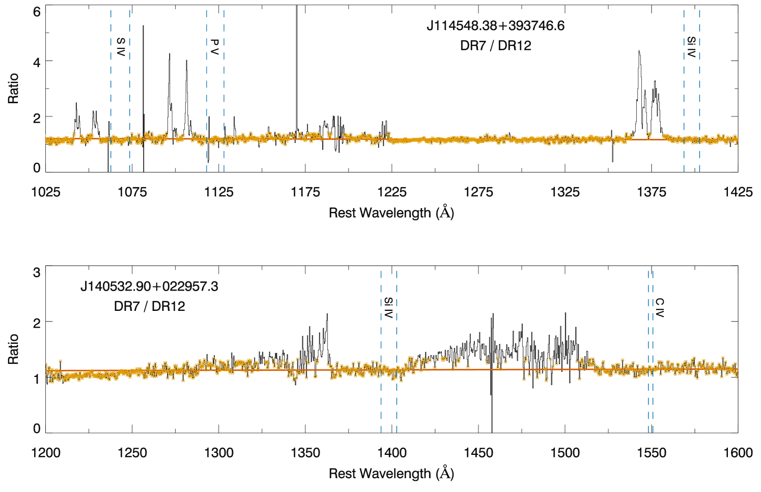
Figure 1: Representative examples of the ratio-fit procedure used for scaling spectra, which involves fitting the ratio between two spectra using non-variable wavelength intervals (see Section 3.1). Each panel lists the BAL quasar name and surveys (DR7 or DR12) associated with the two spectra used for calculating the ratio spectrum (black). Orange data intervals show the wavelength intervals that remained after the sigma-clipping process; these intervals were used to constrain the ratio fit (shown as the red solid line). Features in the displayed ratio spectra that are not associated with orange intervals likely represent absorption line variability. Vertical, blue, dashed lines show the locations of the S iv, P v, Si iv, and C iv doublets in the rest frame of the quasar.

After scaling, one spectrum was subtracted from the other to create a difference spectrum. In order to detect absorption-line variations related to BAL outflows and to avoid detection of spurious changes across individual, unresolved pixels, we binned each difference spectrum by 2000 and 500 km s ^-1. The 2000 km s^-1 bin width is the minimum representative width of a BAL (Weymann et al. 1991), and is utilized to search for BAL variability across wider regions. The 500 km s^-1 bin width is the minimum width that traces high-velocity winds (i.e., the mini-BAL outflows; see e.g. Hamann & Sabra 2004), and is used to search for BAL changes across narrower intervals. The cumulative sigma ($\sigma$) in a given binned difference value was calculated by adding the propagated random and systematic errors in quadrature on a pixel-by-pixel basis (see Fig. 2). Random errors within each bin were propagated in quadrature to determine the random error for each binned difference value. Systematic errors within each bin were averaged as opposed to propagated in quadrature since these uncertainties are not independent and random from one another.

Systematic errors include uncertainties in matching resolutions, wavelength calibration errors in CCDS spectra, and errors in the ratio fits used for scaling. The standard deviation of the width of the Gaussian smoothing function used to match resolutions was estimated to be 68 per cent of the amount between the minimum and maximum resolutions for each instrument. Uncertainties in wavelength for a given CCDS spectrum were estimated using night sky emission lines. Errors in the scaling function were estimated by generating distributions of the residuals between non-rejected ratio values and the fit over localized wavelength intervals. The error in the fit at each wavelength was quantified by adding in quadrature the mean and standard deviation of the mean of the corresponding residual distribution.

BAL variability was determined by comparing binned flux differences with propagated errors, and we categorized each case as N (no), T (tentative), or Y (yes). Binned, absorption-line differences <3$\sigma$, either positive or negative, using both the 2000 and 500 km s^-1 bin widths are categorized as N. Differences between 3 and 4$\sigma$ contaminated by potential emission-line changes are also placed in the N category. Tentative (T) variability constitutes binned, absorption-line differences between 3 and 4$\sigma$ using either the 2000 or the 500 km s^-1 bin widths. Absorption-line differences that are >4$\sigma$ for only 1–2 bins, are very close to the 4$\sigma$ threshold, are potentially contaminated by emission-line changes, and/or generally appear marginal/spurious by eye are also placed in the T category. Variable (Y) binned, absorption-line difference values are >4$\sigma$ over more than 2 consecutive bins using either the 500 or the 2000 km s^-1 bin widths, and appear convincing by eye. If any BAL for a given quasar exhibits variable (Y) absorption-line differences over our measured time-scales, then the variability category for that quasar is Y (the same rule applies to T quasars; see last column of Table 1).

3.2 P v column densities

We utilize the P v BAL, a tracer of high column density gas, to constrain the hydrogen column density of the absorber (see Section 4.3). In order to estimate the P v column density, the P v BAL apparent optical depth profiles were estimated and then integrated over appropriate velocity intervals. The measured P v column densities are lower limits due to potential effects of large optical depths masked by partial coverage of the background light source (e.g., Moravec et al., 2017, and references therein).

The P v BAL apparent optical depths were calculated using the residual fluxes within the troughs [i.e., $\tau=-$ln$(F_{v}/F_{c,v})$], where $F_{v}$ and $F_{c,v}$ are the fluxes of the spectrum and continuum, respectively, at a given velocity $v$. The continuum fluxes were estimated by fitting a power law to either the DR7 or DR12 spectrum in each source and minimizing a $\chi^{2}$ statistic (see Fig. 2). The Si iv, C iv, and Al iii BELs were fitted using Gaussians simultaneously with the power law function. The fits included wavelength intervals that were free of BALs and ranged from approximately 1260–1350, 1370–1480, 1530–1800, and 1870–2500 Å.

We integrated the P v BAL apparent optical depth profiles using the following equation, in Gaussian units:

$$N=\frac{m_{e}c}{\pi e^{2}f\lambda}\int\tau(v)dv$$ (1)

where $f$ is the oscillator strength, $\lambda$ is the rest wavelength, and $\tau(v)$ is the apparent optical depth at a given velocity (Savage & Sembach, 1991). Rest wavelengths and oscillator strength values were taken from Morton (2003), and we treat the P v $\lambda\lambda$1117,1128 doublet as a single line at $\lambda=1121$ Å with an average oscillator strength of $f=0.705$. For sources that showed non-variable P v BALs, we integrated $\tau(v)$ in accordance with equation (1). For sources that showed variable P v BALs, we integrated the optical depth difference to generate lower limits for the change in P v column density.

Table 4: Variable BAL properties

Quasar name	BALs	$\Delta t$	$v_{\mathrm{LOS}}$	Direction
		(yr)	(km s -1)
013652+122501	P v	0.6	–6200	–
025042+003536	Si iv	2.6	–9400	–
	C iv	2.6	–9400	–
102154+051646	C iv	2.0	–23 900	+
104059+055524	Si iv	2.4	–7700	+
104247+061521	Si iv	0.2	–6800	–
114548+393746	N iii	1.5	–5800	+
	O vi	1.5	–11 000	+
	S iv	1.5	–5700	+
	P v	1.5	–5800	+
	H i	1.5	–7100	+
	Si iv	1.5	–5600	+
	C iv	1.5	–7500	+
		1.5	–11 100	+
122654–005430	Si iv	2.4	–3000	+
		0.8	–2500	+
		0.5	–2500	–
	C iv	2.4	–4300	+
		2.4	–9000	+
		2.4	–13 700	+
		2.4	–17 600	+
		0.8	–17 600	+
140532+022947	P v	2.4	–7400	+
	N v	2.4	–24 000	+
		0.8	–18 700	–
	Si iv	2.4	–8900	+
		0.8	–10 200	–
	C iv	2.4	–23 000	+
		0.8	–19 200	–
221326+003846	C iv	2.0	–10 000	+
		0.8	–8100	–
230721+011118	C iv	0.8	–6900	+

Information listed for each BAL quasar includes (from left to right): ions associated with variable BALs, measured time-scales of BAL variability (upper limits that are limited by temporal sampling), LOS velocities corresponding to maximum flux changes within the BALs, and whether the BAL depths increased (+) or decreased (–). Multiple, distinct time-scales listed for the same ion are in chronological order. Multiple velocities for the same time-scale correspond to kinematically separate absorption troughs.

4 Results and Discussion

4.1 Absorption line variability

We detect definite (category Y, see Section 3.1) variability from any BAL (i.e., from C iv, Si iv, or P v) in 10 out of 71 BAL quasars in our sample (see Appendix A for notes on individual objects). Spectroscopic comparisons in our sample probe rest-frame time-scales between 0.5 d and 3.8 yr, and we measure BAL variability time-scales over $\leq$ 0.2–3.8 yr for our Y sources. Tentative (T) variations from any BAL are detected in 44 sources, and 17 objects exhibit no (N) BAL changes. Table 3 lists the associated ion, measured variability time-scale, LOS velocity of the variable region, and variability direction for each variable (Y) BAL in our sample. BALs not presented in Table 3 show no significant absorption line changes over the listed time-scales. For example, there are 4 cases of P v and/or Si iv BAL variations with no associated C iv BAL changes in the same time-scale comparison (see 013652+122501, 104059+055524, 104247+061521, and 0.5 yr for 122654–005430 in Table 3). We detect 4 cases of C iv BAL variability with non-variable P v absorption at similar velocities (see 2.4 yr for 122654–005430, 0.8 yr for 140532+022947, along with 2.0 and 0.8 yr for 221326+003846 in Table 3). There are 5 cases of C iv BAL changes with likely no associated P v absorption at similar velocities (see 102154+051646, 114548+393746, 2.4 and 0.8 yr for 122654–005430, and 2.4 yr for 140532+022947 in Table 3). In 2 cases (025042+003536 and 230721+011118; see Table 3)

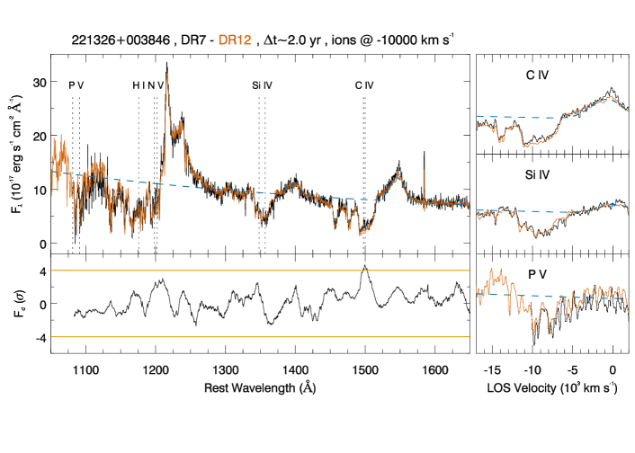
Figure 2: BAL quasar spectroscopic comparisons, revealing BAL variability from a range of ions. Details above the large panel include the BAL quasar name, instruments and colours used for the displayed spectra, rest-frame time-scale between observations, and the blue-shifted velocity of the labelled transitions (vertical, dotted lines). All vertical line labels are at the same velocity, and lie at a velocity that is centered on a variable (Y) interval within the BAL; these line labels do not correspond to the deepest portion of the BAL. The large panel displays two spectra over a large wavelength interval, and the three small panels on the right displays the two spectra in the vicinity of the C iv, Si iv, and P v BALs on a common velocity and flux scale. Spectra in the small panels were smoothed using a 3-pixel wide boxcar for better presentation. The panel below the large panel displays the difference spectrum (in units of $\sigma$, see Section 3.1) for the two spectra, as well as the $\pm 4\sigma$ thresholds (solid orange lines) used for detecting variable (Y) BALs. The order of the difference operation is the order of the instruments listed above the large panel. The dashed blue line in the large panel and small panels is the fit applied to either the DR7 or DR12 epoch and consists of a power law and Gaussians to model the continuum and BELs, respectively. All component figures are available in the online, supplementary material (see Fig. 2S).

it is unclear if the C iv BAL variations are associated with P v absorption at the same velocity.

The 10 Y sources exhibit BAL changes associated with resonance transitions from ions including N iii $\lambda\lambda$989,991, O vi $\lambda\lambda$1031,1037, S iv $\lambda\lambda$1062,1073, P v $\lambda\lambda$1117,1128, H i $\lambda$1215, N v $\lambda\lambda$1238,1242, Si iv $\lambda\lambda$1393,1402, and C iv $\lambda\lambda$1548,1550. Tentative absorption line variability is detected from these transitions as well as from the C ii $\lambda\lambda$1334,1335 and Al iii $\lambda\lambda$1854,1862 doublets. Fig. 2 shows spectroscopic comparisons for each of the 10 BAL quasars listed in Table 3. We note that spectra for 025042+003536 and 104059+055524 presented in Fig. 2 do not allow for variability comparisons of the P v BAL, however other spectra for these sources provide sufficient coverage to search for P v BAL changes (see Table 1). Since there is no BAL variability information to present in these other cases, we therefore do not show all spectroscopic comparisons in Fig. 2.

Previous studies focusing on C iv and Si iv BALs have concluded that BAL variability is common on rest frame time-scales of a few years and therefore a significant fraction of outflows exist within the vicinity of the SMBH (i.e. $\la$100 pc, see e.g. Filiz Ak et al. 2013). Filiz Ak et al. (2013) measured C iv and Si iv BAL equivalent width variations in 291 BAL quasars, finding that approximately 50–60 per cent of the BALs vary over time-scales ranging from 1 to 3.7 yr. Capellupo et al. (2013) concluded that over 50 per cent of their two-epoch comparisons exhibit C iv BAL variability on 1-year time-scales, with a higher probability of detecting BAL changes over multi-year time-scales (see their fig. 9). Our measured BAL variability time-scales are broadly consistent with previous results. The low fraction of BAL quasars in our sample that exhibit significant C iv BAL variations (i.e., $\sim$10 per cent) is consistent with previous studies which conclude that weaker C iv BALs generally vary with greater frequency and with larger fractional EW changes than stronger C iv BALs (see e.g., Capellupo et al. 2011; Filiz Ak et al. 2013); P v BALs in our sample indicate a preference toward detecting strong C iv BALs (see Fig. 2).

In some cases we observe variable BALs associated with more than a single ion increase or decrease together at similar velocities (see e.g., in Fig. 2, the C iv and Si iv BAL variations at –9400 km s^-1 in 025042+003536 as well as BAL variations at roughly –5700 km s^-1 from N iii, S iv, P v, Si iv, and C iv in 114548+393746). We also detect BALs that change their variability direction from one comparison to the next. The BALs associated with N v, Si iv, and C iv in 140532+022947 increase in strength over the first 2.4 yr, then decrease in strength over the next 0.8 yr (see Fig. 2). The C iv BAL in 221326+003846 increases in strength over the first 2.0 yr then decreases in strength over the next 0.8 yr (see Fig. 2). The Si iv BAL in 122654–005430 increases over the first 2.4 yr and the next 0.8 yr, and then decreases in strength over the next 0.5 yr (see Fig. 2).

Understanding the origin of BAL variability is critical to constraining outflow energetics since the constraints we derive on the location of the absorber relative to the SMBH depend on the mechanism that produces the observed BAL variations. We utilize the spectroscopic comparisons in Fig. 2 in conjunction with CSS $V$-band light curves (representative cases are shown in Fig. 3) to interpret the BAL variations in our sample. Below we discuss variability scenarios that provide evidence supporting one of the two scenarios (see Section 1) as the plausible explanation for the detected BAL variability. The origin of BAL variations in most sources in our sample is ambiguous given the limited amount of information available and the unknown geometry of BAL outflows (see e.g., Hamann & Sabra 2004), and we therefore only focus on sources with supporting evidence of one of the two scenarios in the subsequent discussion.

Detecting variability in a C iv BAL that is highly optically thick supports models involving outflows crossing the LOS since a saturated absorber might not respond to fluctuations in the ionizing radiation field in a significant way (see Capellupo et al. 2014). The C iv BAL is likely highly optically thick if P v absorption exists at the same velocity (see Section 1), and we detect significant (Y) variations in 2 highly optically thick C iv BALs with no detectable P v BAL changes at the same velocity. We observe Y variations in the C iv BAL in 221326+003846 over the first 2.0 yr and the following 0.8 yr, and P v broad absorption exists at the same velocity as the observed C iv BAL variability (see Fig. 2). Significant C iv BAL variations are also detected with P v broad absorption at similar velocities in 140532+022957 over a 0.8 yr time-scale (see Fig. 2).

Observing variability in P v and/or Si iv BALs but not in highly optically thick C iv broad absorption at the same velocity supports ionization-change scenarios, since transverse motions would likely alter a highly optically thick C iv BAL profile (see above and Capellupo et al. 2014). We detect Y variations in 6 P v and/or Si iv BALs with no detectable C iv BAL changes at similar velocities. The quasar 013652+122501 exhibits a non-black, non-variable C iv BAL that lies at velocities where P v BAL variability is detected (see Fig. 2). Similarly, we observe a dramatic increase in the Si iv BAL strength in 104059+055524 which exists at the same velocity as a non-black, non-variable C iv BAL that is likely highly optically thick due to the presence of P v broad absorption at the same velocity (see Fig. 2). The Si iv BAL decreases in strength at –6800 km s^-1 in 104247+061521, and this BAL lies at the same velocity as a non-variable C iv BAL with associated P v broad absorption at the same velocity (see Fig. 2). The Si iv BAL decreases in strength at –2500 km s^-1 over 0.5 yr in 122654–005430, and this trough also lies at the same velocity as a non-variable C iv BAL with P v broad absorption at the same velocity (see Fig. 2).

We also see examples of significant, coordinated absorption line variations associated with C iv over a large velocity interval that spans $>10\,000$ km s^-1. Coordinated line variations over a large range of velocity seem to favour variations in the ionizing radiation field, however transverse-motion scenarios cannot be entirely ruled out (Hamann et al. 2011; Capellupo et al. 2013; Grier et al. 2015; Wang et al. 2015). We observe decreases in C iv absorption line depth from four distinct troughs over a –14 300 km s^-1 range between the DR7/DR12 epochs in 122654–005430, and from a single C iv BAL over -12 600 km s^-1 between the DR7/DR12 observations for 140532+0222957 (see Fig. 2 and Table 3).

Fluctuations in the observed continuum flux provide evidence supporting an ionization change occurring within the absorber if a correlation exists between variations in continuum flux and ionizing radiation flux. We inspect the CSS light curves in combination with our detected BAL variability to examine whether any quasars exhibit significant $V$-band variations that are likely mostly due to continuum emission. Fig. 3 displays representative, synthesized $V$-band light curves for our variable (Y) BAL quasars. Three Y sources in our sample exhibit significant (i.e., $\gtrsim 0.5$ mag) CSS variations within the observation time that are likely mostly due to continuum emission (see 104247+061521, 122654–005430 and 221326+003845 in Fig. 3), however three Y objects show marginal (i.e., $\sim$0.2–0.5 mag) CSS variations within the observation time (see 013652+122501, 114548+393746, and 140532+022957). The remaining four Y quasars exhibit poor sampling or small-amplitude (i.e., $\lesssim$0.2 mag) variations in the CSS observations. In light of the mixed behaviour we observe in the CSS light curves across our Y sources, we do not find strong evidence for the sample as a whole supporting the ionization-change scenario.

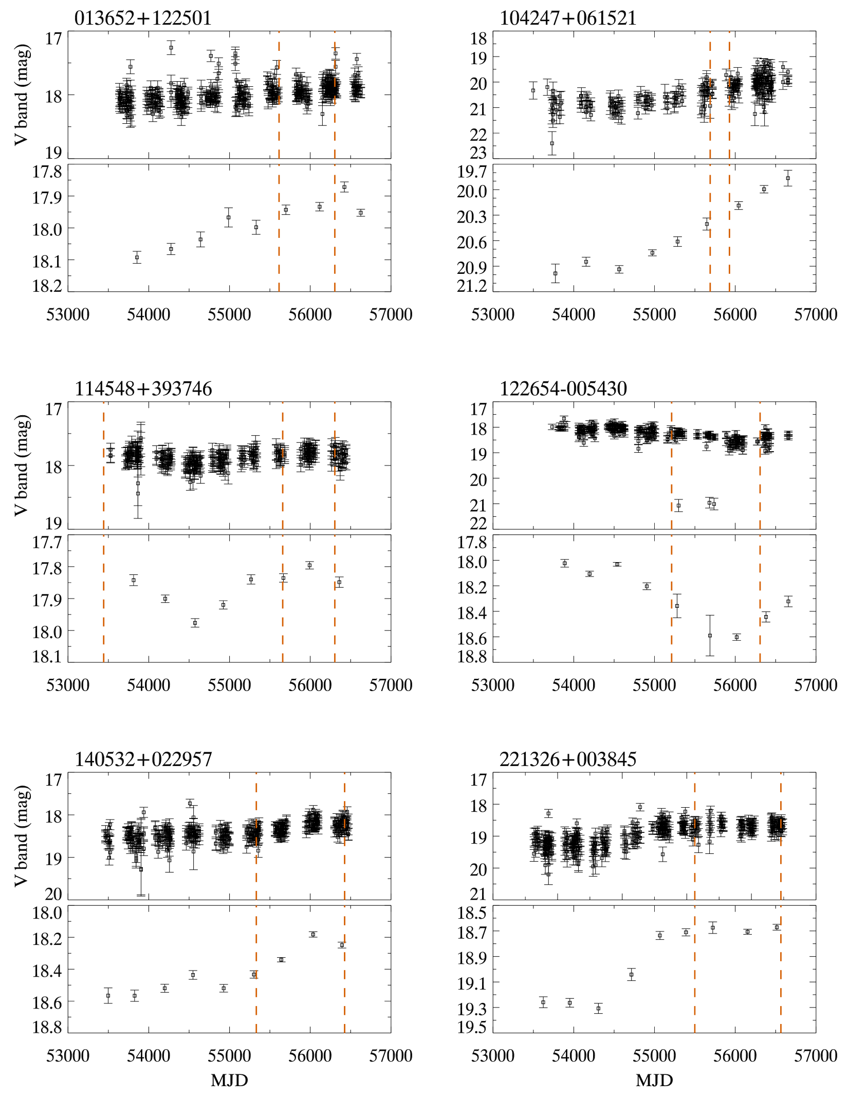
Figure 3: CSS $V$-band light curves, indicating flux variations. The source name is listed above each pair of panels. The upper panel for each source shows all photometric measurements and their errors, and each lower panel shows the mean $V$-band magnitude and standard deviation of the mean over one-year increments. Red dotted lines indicate the epochs of our spectroscopic observations (see Table 1).

4.2 Quasar outflow locations

The BAL variations that we detect in 10 BAL quasars (see Fig. 2 and Table 3) collectively provide evidence supporting scenarios involving motions of gas across the LOS and ionization changes within the absorbers (see Section 4.1). Below we estimate representative BAL outflow distances from the SMBH using both interpretations and discuss our results in the context of previous studies that have constrained quasar outflow distances.

4.2.1 Outflows crossing the LOS

We consider outflowing gas crossing the LOS and use the Keplerian speed in order to obtain a characteristic upper limit for the outflow distance $r$ from the SMBH [i.e. $r=GM_{\bullet}/v_{\mathrm{cross}}^{2}$, where $G$ is the gravitational constant, $M_{\bullet}$ is the SMBH mass (see Table 1), and $v_{\mathrm{cross}}$ is the transverse speed of the absorber across the LOS].

We estimate the transverse speed $v_{\mathrm{cross}}$ using the measured BAL variability time-scale $\Delta t$, the change in absorber covering fraction $\Delta A$, the diameter of the background light source at a specified wavelength $D_{\lambda}$, and the geometries of the absorber and background light source. We utilize an average BAL variability time-scale of $\Delta t\leq 1.22$ yr for our calculation. The $\Delta A$ parameter is quantified as the average, normalized flux difference across the variable wavelength interval within the BAL (see Capellupo et al. 2011), and we assume $\tau>>1$ so the line depth is a direct measure of the covering fraction. We measure an average value of $\Delta A=0.18$ for our variable BALs, with an estimated uncertainty of 30 per cent [i.e., by using the 1$\sigma$ errors for each pair of spectra (see Section 3.1) and by assigning a 20 per cent error to the continuum flux values based on examination of results from alternative fits applied to the spectra].

The size of the background light source $D_{\lambda}$ is calculated using the standard thin-disc temperature profile in combination with Wien’s law (see discussion in section 4.1 of Edelson et al. 2015), and incorporates a modified constant to account for disc-size measurement discrepancies (Hamann et al. in preparation). The size $D_{\lambda}$ depends on $L_{\mathrm{bol}}$ and $M_{\bullet}$ (see Table 1), the radiative efficiency $\eta$, and the wavelength $\lambda$. For our calculation we adopt log $L_{\mathrm{bol}}=47.0$ and log $M_{\bullet}=9.4$ to be representative values for our sample, and the errors for $L_{\mathrm{bol}}$ and $M_{\bullet}$ have been estimated to be $\sim$0.3 and 0.5 dex, respectively, based on systematic uncertainties in using single epoch spectra to measure black hole masses (see e.g., Shen 2013). Using the above measurements along with nominal values of $\eta=0.1$ and $\lambda=1320$ Å, we obtain a continuum source size estimate on the order of $D_{\lambda}=0.01$ pc for our BAL quasar sample.

We adopt the knife-edge geometry from Capellupo et al. (2013) for our calculations of $v_{\mathrm{cross}}$, which consists of a circular absorber of infinite radius crossing a square continuum source. The knife-edge model is used as a conservative, extreme geometry that should encompass the actual, unknown outflow geometries, and leads to a lower limit for the outflow crossing speed (i.e. $v_{\mathrm{cross}}\ga\Delta A\,D_{\lambda}/\Delta t$) and therefore an upper limit on $r$. Our measurements yield a lower limit of $v_{\mathrm{cross}}\ga 1500$ km s^-1 for typical variable BALs in our sample. Using the above considerations, we obtain an upper limit for the BAL outflow distance from the SMBH to be $r\sim$5 pc. Factoring in estimated uncertainties in the above parameters yields a range of distances on the order of $r\la 1-10$ pc for our sample using the Keplerian speed and transverse-motion interpretation.

4.2.2 Outflows undergoing an ionization change

We consider an absorber undergoing an ionization change and constrain the outflow distance $r$ from the SMBH by considering an ionizing radiation field that illuminates a constant-density outflow [i.e. $r=\sqrt{L_{\mathrm{ion}}/(4\pi Un_{\mathrm{e}}c)}$, where $L_{\mathrm{ion}}$ is the ionizing photon luminosity above 13.6 eV, $U$ is the ionization parameter, $n_{\mathrm{e}}$ is the electron density, and $c$ is the speed of light].

The ionizing photon luminosity $L_{\mathrm{ion}}$ above 13.6 eV is calculated by integrating a piece-wise power law ($L_{\nu}=\nu^{\alpha}$) for a typical quasar SED (Hamann et al., 2011) and using measurements of the luminosity at 1350 Å (see Section 2) to normalize the power law function. Hamann et al. (2011) adopted a quasar SED that consists of $\alpha=-1.0$ from 0.5 to 13.6 eV, $\alpha=-2.56$ from 13.6 to 136 eV, and $\alpha=-1.0$ from 136 eV to 136 keV. We obtain an average estimate, in photons s^-1, of log $L_{\mathrm{ion}}=56.8$ for BAL quasars in our sample.

Wang et al. (2015) analysed a large sample of quasars from SDSS DR10, concluding that coordinated BAL variations from C iv, Si iv, and N v are statistically correlated with continuum variations in their sample. They attributed the variability in their sample to be broadly due to changes in the ionizing radiation field and further concluded that the majority of ions present in the absorbers are from higher ionization states than C iv, Si iv, and N v. Wang et al. (2015) conducted photoionization models in conjunction with their results and constrained the ionization parameter for their BAL outflows to be log $U\ga 0$. Based on the applicability of these results to BAL quasars more generally, we adopt the lower limit of log $U\ga 0$ for our calculation.

The electron density is constrained by utilizing the measured BAL variability time-scale $\Delta t$ as an upper limit to the recombination time-scale of the gas; an upper limit on the recombination time yields a lower limit on the electron density (i.e. $n_{\mathrm{e}}\ga 1/\alpha_{\mathrm{rec}}\Delta t$, where $\alpha_{\mathrm{rec}}$ represents the recombination rate coefficient). We calculate $\alpha_{\mathrm{rec}}$ for the relevant ions of interest using version 8.0 of the CHIANTI atomic database (Dere et al. 1997; Del Zanna et al. 2015), using a nominal temperature of 20 000 K for the BAL gas. We caution that constraining the electron density in this way does not account for the unknown ionization conditions in the BAL gas (see e.g., Hamann et al. 1997), however our results are still useful for the purpose of obtaining order-of-magnitude limits on the outflow distance. We utilize average values of $\Delta t\leq 1.22$ yr and $\alpha_{\mathrm{rec}}=2.0\times 10^{-11}$ cm³ s^-1 to obtain a nominal lower limit of $n_{\mathrm{e}}\ga 1300$ cm^-3. Using the above considerations and uncertainties, we estimate an upper limit for the BAL outflow distance from the SMBH to be $r\sim$350 pc and a range on the order of $r\la 100-1000$ pc using the ionization-change scenario.

4.2.3 Comparisons to previous work

Our BAL outflow distance constraints using the transverse-motion scenario (i.e., $r\la 1-10$ pc; see Section 4.2.1) and the ionization-change interpretation (i.e., $r\la 100-1000$ pc; see Section 4.2.2) indicate that we may be probing outflowing gas in close proximity to the SMBH, but the possibility remains that outflows in our sample exist at larger scales. We emphasize that these upper limits leaves open the possibility that the absorbers we probe are located at small distances from the SMBH under the ionization-change scenario. Below we compare our results to previous observational studies that have constrained quasar outflow distances.

Previous quasar outflow distance constraints using BAL variability studies are broadly consistent with our results. Capellupo et al. (2011, 2012, 2013) detected C iv and Si iv BAL variability and constrained the outflows in their sample to lie within $\sim$10 pc of the SMBH by attributing the variations to absorbers crossing the LOS. Capellupo et al. (2013) also detected C iv BAL changes on rapid time-scales, allowing them to constrain the absorber to lie between 0.001 and 0.02 pc of the SMBH. Capellupo et al. (2014) found BAL variability associated with P v, Si iv, and C iv at the same velocity in Q1413+1143, thereby providing strong support for absorbers crossing the LOS and allowed them to place an upper limit of $\sim$3.5 pc for the outflow distance from the SMBH. Variability studies involving Fe ii and Mg ii BALs have constrained quasar outflows to lie within tens of parsecs of the SMBH by using the crossing absorber interpretation (Hall et al. 2011; McGraw et al. 2015). Barlow (1994) examined the variability patterns of C iv, N v, Si iv, and Al iii BALs, yielding upper limits on the outflow distance to be a few hundred parsecs from the SMBH based on an ionization change scenario (see also Vivek et al. 2012).

Studies of quasar outflows have also utilized photoionization models in conjunction with density-sensitive absorption lines to constrain outflow distances that are generally $\ga$100 pc from the SMBH. Previous work using ground- and excited-state transitions in O iv to constrain the gas density have estimated outflow distances of 3 kpc (Arav et al., 2013) from the SMBH. The S iv ion also allows for density constraints, leading to outflow distances of $\sim$100 pc (Chamberlain et al. 2015) and between 100 and 2000 pc (Borguet et al., 2013) from the SMBH. Other studies have utilized the Si ii ion to estimate large outflow distances of 6 kpc in an iron low-ionization BAL quasar (Dunn et al., 2010). Chamberlain & Arav (2015) utilized the N iii and S iii absorption lines in LBQS J1206+1052 to estimate the outflow distance to be $\sim$840 pc from the SMBH.

In light of the above discussion, it is possible that quasar outflows exist at a range of distances from the SMBH. This conclusion suggests that quasar outflows might exhibit a range of energies and momenta and therefore some outflows may play a significant role in AGN feedback processes. We obtain nominal estimates on the energetics of BAL outflows in our sample (see Section 4.4) and discuss our results in the context of previous studies.

4.3 Quasar outflow hydrogen column densities

We obtain an average lower limit on the P v column density to be log $N_{\text{P\,{v}}}\ga 15.1$ based on our spectroscopic fits and integration routines (see Section 3.2), and consider this constraint to be representative of BAL outflows in our sample. Hamann (1998) carried out photoionization simulations of the BAL quasar PG 1254+047 and utilized his measured P v column density lower limit of log $N_{\text{P\,{v}}}=15.0$ to estimate the hydrogen column density of the flow to be log $N_{\mathrm{H}}\ga 22.0$, assuming solar abundances and constant-density clouds.

Leighly et al. (2009) applied a template-fitting approach to the emerging BAL AGN WPVS 007 to measure a P v column density of log $N_{\text{P\,{v}}}\sim 15.4$ and used photoionization models to estimate a hydrogen column density of log $N_{\mathrm{H}}\geq 22.2$ assuming solar abundances and an SED determined by using UV/optical spectra and $Swift$ X-ray observations. Borguet et al. (2012) utilized a measured P v column density of log $N_{\text{P\,{v}}}\sim 14.6$ in conjunction with S iv to estimate a hydrogen column density of log $N_{\mathrm{H}}=21.9$ in the BAL quasar SDSS J1512+1119.

In light of previous results, we adopt the ratio log $N_{\mathrm{H}}$/log $N_{\text{P\,{v}}}>7.0$ from Hamann (1998) to estimate a nominal, average lower limit of log $N_{\mathrm{H}}\ga 22.1$ for BAL outflows in our sample. Of the previous studies above that place observational constraints on outflow column densities, we adopt the Hamann (1998) parameters to use as representative values for obtaining order-of-magnitude estimates of outflow energetics. The nominal values we adopt are consistent with Leighly et al. (2011) who analysed a range of BAL outflow ionization conditions using photoionization models, and concluded that the P v lines do not become prominent until the absorber exhibits high column densities on the order of log $N_{\mathrm{H}}\sim$22.0–23.0 assuming solar abundances (see their fig. 15).

4.4 Quasar outflow energetics

We quantify BAL outflow energetics by calculating the mass flow rate $\dot{M}_{\mathrm{out}}$, kinetic luminosity $L_{\mathrm{k}}$, and momentum flux $\dot{P}$ for variable (Y) BALs in our sample. These parameters depend on measurements of the outflow LOS velocity $v_{\textrm{LOS}}$ (see Table 3), outflow hydrogen column density $N_{\mathrm{H}}$, outflow distance $r$ from the SMBH (see Sections 4.2.1 and 4.2.2), and outflow global covering fraction $Q$. For the subsequent calculations we adopt a value of log $N_{\mathrm{H}}=22.1$ based on our P v column density measurements (see Sections 3.2 and 4.3), a nominal value of $Q=15$ per cent based on the observed fraction of BAL quasars (see e.g., Trump et al. 2006), and a representative value of $v_{\rm{LOS}}=10\,000\,$ km s^-1 based on our BAL velocity measurements.

The average mass flow rate is calculated using a characteristic flow time (i.e., $t_{\mathrm{flow}}=r/v_{\mathrm{LOS}}$) along with an estimate of the outflow mass $M_{\mathrm{out}}$, and is quantified as $\dot{M}_{\mathrm{out}}=M_{\mathrm{out}}/t_{\mathrm{flow}}$. The mass of the outflow is obtained by assuming a thin-shell geometry and is calculated using the following equation:

$$M_{\mathrm{out}}\approx 4100\Big{(}\frac{Q}{15\%}\Big{)}\Big{(}\frac{N_{\mathrm{H}}}{2\times 10^{22}\,\mathrm{cm}^{-2}}\Big{)}\Big{(}\frac{r}{3.5\mathrm{pc}}\Big{)}^{2}\ M_{\odot}$$ (2)

where the parameters are defined above [see equation (2) from Capellupo et al. 2014]. For comparison we also estimate the accretion rate $\dot{M}_{\mathrm{acc}}$ using our representative value of $L_{\mathrm{bol}}=47.0$ and a radiative efficiency of $\eta=$0.1 [i.e. $\dot{M}_{\mathrm{acc}}=L_{\mathrm{bol}}/(\eta c^{2}$)]. Using the above parameters we calculate the kinetic luminosity [$L_{\mathrm{k}}=(1/2)\dot{M}_{\mathrm{out}}v_{\textrm{LOS}}^{2}$] and momentum flux ($\dot{P}=\dot{M}_{\mathrm{out}}v_{\textrm{LOS}}$) in units of $L_{\mathrm{bol}}$ and $L_{\mathrm{bol}}/c$, respectively. We utilize the above values and consider a BAL outflow located at $r=1,10,100,1000$ pc from the SMBH, consistent with representative distances we estimate using the transverse-motion and ionization-change interpretations, and calculate outflow energetics using these four nominal locations; Table 4 lists the results.

Table 5: BAL outflow energetics

$r$	$M_{\mathrm{out}}$	$t_{\mathrm{flow}}$	$\dot{M}_{\mathrm{out}}$	$\dot{M}_{\mathrm{acc}}$	$L_{\mathrm{k}}$	$\dot{P}$
(pc)	($M_{\odot}$)	(yr)	($M_{\odot}\,\mathrm{yr}^{-1}$)	($M_{\odot}\,\mathrm{yr}^{-1}$)	($L_{\mathrm{bol}}$)	($L_{\mathrm{bol}}/c$)
1	100	100	1	10	0.001	0.01
10	1$\times 10^{4}$	1000	10	10	0.01	0.1
100	1$\times 10^{6}$	1$\times 10^{4}$	100	10	0.1	1
1000	1$\times 10^{8}$	1$\times 10^{5}$	1000	10	1	10

Information listed for each quasar includes (from left to right): Assumed BAL outflow distance from the SMBH, outflow mass, characteristic flow time, mass flow rate, mass accretion rate, kinetic luminosity (in units of $L_{\mathrm{bol}}$), and momentum flux (in units of $L_{\mathrm{bol}}/c$).

In order to assess the viability of the outflows in our sample to contribute to AGN feedback it is necessary to make comparisons to proposed thresholds for outflows to become energetic enough to affect the host galaxy. Previous work has generally concluded that an outflow with a kinetic luminosity of $\sim$0.05 $L_{\mathrm{bol}}$ can significantly accelerate ISM gas (see e.g., King & Pounds 2015). Hopkins & Elvis (2010) noted that the above threshold assumes that the outflowing gas affects all phases of the ISM, leading them to propose decreases in the above threshold to $\sim$0.005 $L_{\mathrm{bol}}$ by arguing that outflows need only drive the hot, diffuse gas to affect host galaxy properties.

Our estimates of $L_{\mathrm{k}}$ listed in Table 4 are crude approximations for the outflow energetics due to their large uncertainties, partly because the calculations involve multiplying hydrogen column density lower limits by outflow distance upper limits. However our order-of-magnitude energetics estimates using a range of distances can be broadly compared to the proposed $\sim$0.005–0.05 $L_{\mathrm{bol}}$ thresholds outlined above. If a significant number of the BAL outflows in our sample exists in close proximity to the SMBH (i.e., within 10 pc), then it is possible that these winds may only marginally contribute to AGN feedback processes. Conversely if a large number of BAL outflows are located much farther from the SMBH (i.e., 100–1000 pc), then it is possible that these winds would contain sufficient amounts of energy and momentum to contribute to feedback.

Our nominal kinetic luminosity estimates in Table 4 range from 0.001 to 1 $L_{\mathrm{bol}}$, which is broadly consistent with previous studies that utilized independent methodologies to estimate outflow energetics. Other studies have estimated kinetic luminosities on the order of 0.001 (Dunn et al., 2010) and 0.01 $L_{\mathrm{bol}}$ (Moe et al. 2009; Arav et al. 2013; Capellupo et al. 2014). Larger values of $L_{\mathrm{k}}$ have been estimated near the proposed threshold for feedback of 0.05 $L_{\mathrm{bol}}$ (Borguet et al., 2013). Our results indicate that many BAL outflows in our sample possess kinetic energies that are viable for AGN feedback processes.

5 Conclusions

We analyse multiple-epoch spectra of 71 BAL quasars that exhibit conservative detections of the P v $\lambda\lambda$1117,1128 BAL, and find significant variability in 10 sources using quantitative criteria. Our measured rest frame BAL variability time-scales range from $\leq 0.2-3.8$ yr, and variable wavelength intervals are associated with a range of ions including N iii, O vi, S iv, P v, H i, N v, Si iv, and C iv. Our results are consistent with previous work with regard to BAL variability time-scale, velocity, and direction.

We interpret the variable BALs in our sample and find sources that provide evidence supporting transverse motions of gas or ionization changes as explanations for the origin of the detected BAL changes (see Section 4.1). In particular, detecting significant variability in a saturated C iv BAL is evidence supporting an absorber crossing the LOS. We also find evidence supporting an ionization change scenario by detecting significant variability in only the P v and/or Si iv BAL and by identifying coordinated C iv absorption line variability over large velocity intervals. Future high-resolution observations focusing on absorption lines from multiple ions and doublets with large wavelength separations such as the P v $\lambda\lambda$1117,1128, Si iv $\lambda\lambda$1393,1402, and Al iii $\lambda\lambda$1854,1862 BALs will be useful in probing the origin of BAL changes over localized velocity intervals.

Using simple models involving an outflow crossing the LOS, we conclude that BAL outflows in our sample nominally exist on the order of $r\la 1-10$ pc from the SMBH. Under the ionization change interpretation, the BAL outflows we probe are constrained to exist on the order of $r\la 100-1000$ pc from the SMBH. Obtaining multiple-epoch spectra over shorter rest frame time-scales will be necessary for placing more reliable constraints on outflow locations, which will have important implications for the derived feedback-related quantities.

We utilize our quasar outflow distance constraints in conjunction with hydrogen column density limits to estimate kinetic luminosities ranging from 0.001 to 1 times $L_{\mathrm{bol}}$ for outflows in our sample, implying that many quasar outflow energies in our sample are viable for AGN feedback. Our results provide a significant increase in the available information on quasar outflow energetics.

Future studies that focus on absorbers with a range of distances and column densities will be important to better understand the role of quasar outflows in AGN feedback. This work probes high column density outflows using the P v BAL and constrains outflowing gas locations using the BAL variability technique. Utilizing the S iv and Al iii BALs in particular will trace a broader range of column densities, and will give us a more complete picture of quasar outflow demographics when used in conjunction with BAL variability studies.

Appendix A Notes on Individual Quasars

Below we briefly discuss 3 out of 10 BAL quasars that exhibit significant (Y) BAL variability in our sample (see Section 3.1 and Table 3). These three sources exhibit absorption-line changes that are the least convincing of our Y sources, and we outline reasons why the detected variations are plausibly real; the Y quasars not mentioned here show convincing absorption-line variability.

013652+122501

We detect significant variability in the P v BAL at –6200 km s ^-1 between the DR12 and MDM observations (see Fig. 2). The variability is localized (i.e. occurs over a $\sim$10 Å wide region) and is therefore likely not due to fluctuations in continuum emission that would exhibit changes over a large portion of the wavelength coverage (i.e. $\gtrsim$1000 Å). The variability is located at wavelengths that are probably not associated with nearby BELs that could also produce significant variations. The variable wavelength interval is therefore reasonably due to absorption. The flux change is plausibly real since it is greater than 4$\sigma$ over several pixels, is not contaminated by night sky lines, and we observe good agreement between the spectra on either side of the P v BAL (i.e., between –11 000 and –9000 km s^-1 and between –2000 and 0 km s^-1).

102154+051646

We detect a significant C iv absorption line depth increase at –23 900 km s^-1 between the DR7 and DR12 epochs (see Fig. 2). This flux change is localized and lies well outside regions that would be confused by BEL changes, and exists within a high-velocity C iv trough. The flux variations is above 4$\sigma$ over many consecutive pixels and we observe good agreement on either side of the variable interval (i.e., less than –25 000 km s^-1 and greater than –21 000 km s^-1).

The C iv BAL centered at approximately –6000 km s^-1 appears saturated, and there is likely P v broad absorption at similar velocities (see Fig. 2). It is unclear whether the observed C iv absorption line increase at –23 900 km s^-1 has associated P v absorption; the broad absorption feature centered at –20 000 km s^-1 in the P v velocity plot in Fig. 2 is likely attributed to a S iv $\lambda\lambda$1062,1073 BAL.

221326+003846

The C iv BAL exhibits a significant flux increase at –10 000 km s^-1 between the DR7 and DR12 observations, followed by a flux decrease at –8100 km s^-1 between the DR12 and MDM epochs (see Fig. 2). Both of these variable regions are localized and within a C iv BAL that is significantly detached from the nearby C iv BEL, indicating that the variations are likely due to absorption. Both variations are apparent by eye (i.e., due to the the good agreement in flux on either side of the C iv BAL), and exhibit flux differences that are greater than 4$\sigma$ over several consecutive pixels.

Appendix B X-ray observations of 122654–005430

X-ray spectroscopic observations are useful for studying the highly-ionized component of quasar outflows that are not traced by rest frame UV BALs. One source in our sample, 122654–005430, was observed on MJD 52708 using the ACIS instrument onboard the $Chandra$ X-ray Observatory, and we use these observations to extract information on the X-ray spectroscopic shape and degree of absorption in this source. 122654–005430 was observed for 20 800 s and 49 source counts were detected over an energy range of 0.5–7 keV.

The X-ray spectroscopic shape and strength of absorption in 122654–005430 is characterized by comparing observed hardness ratios (H–M)/(H+M) and (M–S)/(M+S) to predicted values to determine the power law photon index $\Gamma$ (i.e. $f_{\mathrm{E}}\propto E^{-\Gamma}$) and intrinsic absorber column density $N_{\mathrm{H}}$. Observed hardness ratios were calculated using the bayesian code from Park et al. (2006) and predicted hardness ratios were generated using the $Chandra$ Portable, Interactive Multi-Mission Simulator (PIMMS) tool. Predicted hardness ratios were determined by varying $\Gamma$ and $N_{\mathrm{H}}$ and were normalized using the H band count rate for 122654–005430. Our predictions include a foreground absorber with column density 2.1$\times 10^{20}$ cm^-2 that was calculated using the Galactic H i maps from Dickey & Lockman (1990).

From the observations we calculate hardness ratios for 122654–005430 to be (H–M)/(H+M)$=-0.51^{+0.15}_{-0.16}$ and (M–S)/(M+S)$=0.19^{+0.16}_{-0.16}$ at 95 per cent confidence, which is consistent with a photon index of $\Gamma\sim 3$ and an intrinsic absorber column density of log $N_{\mathrm{H}}\sim 23$. Our value of $\Gamma\sim 3$ is steeper than results from Gallagher et al. (2002), who measured an average X-ray continuum index of $\Gamma\sim 2$ for their BAL quasar sample. George et al. (2000) obtained a range of X-ray slopes between $1.5\la\Gamma\la 3$ and an average index of $\Gamma\sim 2$ for their sample of non-BAL quasars. Our extracted intrinsic column density of log $N_{\mathrm{H}}\sim 23$ is consistent with previous work that derived X-ray absorber column densities between log $N_{\mathrm{H}}\sim 22-24$ for BAL quasars (Gallagher et al., 2006).

We also investigate the relationship between X-ray and UV flux by calculating the difference between the observed and predicted values of the two point optical-to-X-ray power law index $\alpha_{\mathrm{ox}}$ [i.e. $\Delta\alpha_{\mathrm{ox}}=\alpha_{\mathrm{ox}}(\mathrm{observed})-\alpha_{\mathrm{ox}}(\mathrm{predicted})$]. The observed value of $\alpha_{\mathrm{ox}}$ is defined as 0.384 log ($f_{\mathrm{2\,keV}}/f_{\mathrm{2500\,A}})$, where $f_{\rm{2\,keV}}$ and $f_{\mathrm{2500\,A}}$ are the flux densities at rest-frame 2 keV and 2500 Å, respectively. The flux density at 2 keV is a measure of the absorption-free continuum and was determined with PIMMS using the H band count rate to estimate the flux density at 7 keV and assuming a power law index $\Gamma=3$. The predicted value of $\alpha_{\mathrm{ox}}$ is estimated from the $\alpha_{\mathrm{ox}}-L_{\mathrm{2500\,A}}$ relation for non-BAL quasars from Strateva et al. (2005) [see their equation (6)], where $L_{\mathrm{2500\,A}}$ is the luminosity density at 2500 Å. For the purpose of making comparisons to Gallagher et al. (2006), we do not correct our measured $f_{2500\,A}$ value for Galactic extinction; reddening due to foreground absorbers has the effect of decreasing $\alpha_{\mathrm{ox}}$ and $\Delta\alpha_{\mathrm{ox}}$ by up to $\sim$0.09 and 0.06, respectively (see discussion in section 3 of Gallagher et al. 2006).

We calculate $\alpha_{\mathrm{ox}}$ and $\Delta\alpha_{\mathrm{ox}}$ values of –1.35 and +0.33, respectively, for 122654–005430. Our result is larger than Gallagher et al. (2006) who derived an average value of $\Delta\alpha_{\mathrm{ox}}(\mathrm{corr})\sim-0.10$ for their sample of 35 BAL quasars. Gibson et al. (2009) quantified $\Delta\alpha_{\mathrm{ox}}$ for 166 non-BAL quasars to be on average 0.00$\pm$0.01, which includes corrections for Galactic extinction at rest-frame 2500 Å. We conclude that 122654–005430 exhibits X-ray absorption consistent with previous studies of BAL quasars, but shows a ratio of X-ray-to-UV flux levels that is larger than typically found in previous studies of BAL and non-BAL quasars.

References

- Arav et al. (1999) Arav N., Korista K.T., de Kool M., Junkkarinen V.T., Begelman M.C., 1999, ApJ, 516, 27
- Arav et al. (2001) Arav N. et al., 2001, ApJ, 561, 118
- Arav et al. (2013) Arav N., Borguet B., Chamberlain C., Edmonds D., Danforth C., 2013, MNRAS, 436, 3286
- Asplund et al. (2009) Asplund M., Grevesse N., Sauval A.J., Scott P., 2009, ARA&A, 47, 481
- Barlow (1994) Barlow T. A., 1994, PASP, 106, 548
- Blackburne et al. (2011) Blackburne J.A., Pooley D., Rappaport S., Schechter P.L., 2011, ApJ, 729, 34
- Borguet et al. (2012) Borguet B.C.J., Edmonds D., Arav N., Benn C., Chamberlain C., 2012, ApJ, 758, 69
- Borguet et al. (2013) Borguet B.C.J., Arav N., Edmonds D., Chamberlain C., Benn C., 2013, ApJ, 762, 49
- Capellupo et al. (2011) Capellupo D.M., Hamann F., Shields J.C., Rodríguez Hidalgo P., Barlow T.A., 2011, MNRAS, 413, 908
- Capellupo et al. (2012) Capellupo D.M., Hamann F., Shields J.C., Rodríguez Hidalgo P., Barlow T.A., 2012, MNRAS, 422, 3249
- Capellupo et al. (2013) Capellupo D.M., Hamann F., Shields J.C., Halpern J.P., Barlow T.A., 2013, MNRAS, 429, 1872
- Capellupo, Hamann & Barlow (2014) Capellupo D.M., Hamann F., Barlow T.A., 2014, MNRAS, 444, 1893
- Capellupo et al. (2017) Capellupo D. M. et al., 2017, MNRAS, 469, 323
- Cardelli, Clayton & Mathis (1989) Cardelli J.A., Clayton G.C., Mathis J.S., 1989, ApJ, 345, 245
- Chamberlain & Arav (2015) Chamberlain C., Arav N., 2015, MNRAS, 454, 675
- Chamberlain, Arav & Benn (2015) Chamberlain C., Arav N., Benn C., 2015, MNRAS, 450, 1085
- de Kool & Begelman (1995) de Kool M., Begelman M.C., 1995, ApJ, 455, 448
- Del Zanna et al. (2015) Del Zanna G., Dere K.P., Young P.R., Landi E., Mason H.E., 2015, A&A, 582, A56
- Dere et al. (1997) Dere K.P., Landi E., Mason H.E., Monsignori Fossi B.C., Young P.R., 1997, A&AS, 125, 149
- Dickey & Lockman (1990) Dickey J.M., Lockman F.J., 1990, ARA&A, 28, 215
- Drake et al. (2009) Drake A. J. et al., 2009, ApJ, 696, 870
- Dunn et al. (2010) Dunn J. P. et al., 2010, ApJ, 709, 611
- Edelson et al. (2015) Edelson R. et al., 2015, ApJ, 806, 129
- Evans et al. (2010) Evans I. N. et al., 2010, ApJS, 189, 37
- Everett, Königl & Arav (2002) Everett J., Königl A., Arav N., 2002, ApJ, 569, 671
- Fabian (2012) Fabian A. C., 2012, ARA&A, 50, 455
- Faucher-Giguère & Quataert (2012) Faucher-Giguère C.-A., Quataert E., 2012, MNRAS, 425, 605
- Faucher-Giguère, Quataert & Murray (2012) Faucher-Giguère C.-A., Quataert E., Murray N., 2012, MNRAS, 420, 1347
- Ferrarese & Merritt (2000) Ferrarese L., Merritt D., 2000, ApJ, 539, L9
- Filiz Ak et al. (2013) Filiz Ak N. et al., 2013, ApJ, 777, 168
- Fukumura et al. (2010) Fukumura K., Kazanas D., Contopoulos I., Behar E., 2010, ApJ, 723, L228
- Gallagher et al. (2002) Gallagher S.C., Brandt W.N., Chartas G., Garmire G.P., 2002, ApJ, 567, 37
- Gallagher et al. (2006) Gallagher S.C., Brandt W.N., Chartas G., Priddey R., Garmire G.P., Sambruna R.M., 2006, ApJ, 644, 709
- Gaskell (2007) Gaskell M., 2007, RMxAC, 32, 1
- Gebhardt et al. (2000) Gebhardt K. et al., 2000, ApJ, 539, L13
- George et al. (2000) George I.M., Turner T.J., Yaqoob T., Netzer H., Laor A., Mushotzky R.F., Nandra K., Takahashi T., 2000, ApJ, 531, 52
- Gibson et al. (2009) Gibson R.R., Brandt W.N., Gallagher S.C., Schneider D.P., 2009, ApJ, 696, 924
- Grier et al. (2015) Grier C. J. et al., 2015, ApJ, 806, 111
- Hall et al. (2011) Hall P.B., Anosov K., White R.L., Brandt W.N., Gregg M.D., Gibson R.R., Becker R.H., Schneider D.P., 2011, MNRAS, 411, 2653
- Hamann (1998) Hamann F., 1998, ApJ, 500, 798
- Hamann (1999) Hamann F., 1999, ASP Conf. Ser., 175, 33
- Hamann & Sabra (2004) Hamann F., Sabra B., 2004, ASP Conf. Ser., 311, 203
- Hamann et al. (1997) Hamann F., Barlow T.A., Junkkarinen V., Burbidge B.M., 1997, ApJ, 478, 80
- Hamann et al. (2001) Hamann F.W., Barlow T.A., Chafee F.C., Foltz C.B., Weymann R.J., 2001, ApJ, 550, 142
- Hamann et al. (2011) Hamann F., Kanekar N., Prochaska J.X., Murphy M.T., Ellison S., Malec A.L., Milutinovic N., Ubachs W., 2011, MNRAS, 410, 1957
- Harris et al. (2016) Harris D. W. et al., 2016, AJ, 151, 155
- Hewett & Wild (2010) Hewett P.C., Wild V., 2010, MNRAS, 405, 2302
- Hopkins & Elvis (2010) Hopkins P.F., Elvis M., 2010, MNRAS, 401, 7
- King & Pounds (2015) King A., Pounds K., 2015, ARA&A, 53, 115
- Kormendy & Ho (2013) Kormendy J., Ho L.C., 2013, ARA&A, 51, 511
- Leighly et al. (2009) Leighly K.M., Hamann F., Casebeer D.A., Grupe D., 2009, ApJ, 701, 176
- Leighly, Dietrich & Barber (2011) Leighly K.M., Dietrich M., Barber S., 2011, ApJ, 728, 94
- Lucy et al. (2014) Lucy A.B., Leighly K.M., Terndrup D.M., Dietrich M., Gallagher S.C., 2014, ApJ, 783, 58
- McGraw et al. (2015) McGraw S.M., Shields J.C., Hamann F.W., Capellupo D.M., Gallagher S.C., Brandt W.N., 2015, MNRAS, 453, 1379
- Moe et al. (2009) Moe M., Arav N., Bautista M.A., Korista K.T., 2009, ApJ, 706, 525
- Moravec et al. (2017) Moravec E.A., Hamann F., Capellupo D.M., McGraw S.M., Shields J.C., Rodríguez Hidalgo P., 2017, MNRAS, 468, 4539
- Morton (2003) Morton D. C., 2003, ApJS, 149, 205
- Murray et al. (1995) Murray N., Chiang J., Grossman S.A., Voit G.M., 1995, ApJ, 451, 498
- Pâris et al. (2014) Pâris I. et al., 2014, A&A, 563, A54
- Park et al. (2006) Park T., Kashyap V.L., Siemiginowska A., van Dyk D.A., Zezas A., Heinke C., Wargelin B.J., 2006, ApJ, 652, 610
- Proga & Kallman (2004) Proga D., Kallman T.R., 2004, ApJ, 616, 688
- Proga, Stone & Kallman (2000) Proga D., Stone J.M., Kallman T.R., 2000, ApJ, 543, 686
- Richards et al. (2011) Richards G. T. et al., 2011, AJ, 141, 167
- Savage & Sembach (1991) Savage B.D., Sembach K.R., 1991, ApJ, 379, 245
- Scannapieco & Oh (2004) Scannapieco E., Oh S.P., 2004, ApJ, 608, 62
- Schlegel, Finkbeiner & Davis (1998) Schlegel D.J., Finkbeiner D.P., Davis M., 1998, ApJ, 500, 525
- Shen (2013) Shen Y., 2013, Bull. Astr. Soc. India, 41, 61
- Shen et al. (2011) Shen Y. et al., 2011, ApJS, 194, 45
- Strateva et al. (2005) Strateva I.V., Brandt W.N., Schneider D.P., Vanden Berk D.G., Vignali C., 2005, ApJ, 130, 387
- Trump et al. (2006) Trump J. R. et al., 2006, ApJS, 165, 1
- Vivek et al. (2012) Vivek M., Srianand R., Petitjean P., Noterdaeme P., Mohan V., Mahabal A., Kuriakose V.C., 2012, MNRAS, 423, 2879
- Wang et al. (2015) Wang T., Yang C., Wang H., Ferland G., 2015, ApJ, 814, 150
- Weymann et al. (1991) Weymann R.J., Morris S.L., Foltz C.B., Hewett P.C., 1991, ApJ, 373, 23
- Zhang et al. (2015) Zhang S. et al., 2015, ApJ, 803, 58