Mobile bound states of Rydberg excitations in a lattice

Abstract

Spin lattice models play central role in the studies of quantum magnetism and non-equilibrium dynamics of spin excitations – magnons. We show that a spin lattice with strong nearest-neighbor interactions and tunable long-range hopping of excitations can be realized by a regular array of laser driven atoms, with an excited Rydberg state representing the spin-up state and a Rydberg-dressed ground state corresponding to the spin-down state. We find exotic interaction-bound states of magnons that propagate in the lattice via the combination of resonant two-site hopping and non-resonant second-order hopping processes. Arrays of trapped Rydberg-dressed atoms can thus serve as a flexible platform to simulate and study fundamental few-body dynamics in spin lattices.

Introduction.

Interacting many-body quantum systems are notoriously difficult to simulate on classical computers, due to the exponentially large Hilbert space and quantum correlations between the constituents. It was therefore suggested to simulate quantum physics with quantum computers Feynman (1982), or universal quantum simulators consisting of spin lattices with tunable interactions between the spins Lloyd (1996). Dynamically controlled spin lattices can realize digital and analog quantum simulations. Quantum field theories not amenable to perturbative treatments are often discretized and mapped onto the lattice models for numerical calculations. Spin lattices are fundamental to the studies of many solid state systems, where the competition between the interaction and kinetic energies determines such phenomena as magnetism and superconductivity.

Realizing tunable spin lattices in the quantum regime is challenging. Several systems are being explored to this end, including trapped ions Blatt and Roos (2012); Zhang et al. (2017), superconducting circuits Houck et al. (2012); Neill et al. (2017), quantum dots Hensgens et al. (2017) and other solid state systems. Cold atoms in optical lattice potentials are accurately described by the Hubbard model, representing perhaps the most versatile and scalable platform to realize various lattice models Gross and Bloch (2017). The Hubbard model for two-state fermions or strongly interacting bosons at half filling can implement the lattice spin-1/2 model Kuklov and Svistunov (2003); Duan et al. (2003). The spin-exchange interaction then stems from the second-order tunneling (superexchange) process Trotzky et al. (2008); Chen et al. (2011) and the interspin Ising interaction can exist for atoms or molecules with static magnetic or electric dipole moments Lahaye et al. (2009); Moses et al. (2017). These interactions are, however, weak (tens of Hz or less), which makes the system vulnerable to thermal effects even at ultra-low temperatures of nK Greif et al. (2013); Boll et al. (2016); Mazurenko et al. (2017).

Here we propose a practical realization of a tunable spin lattice $XXZ$ model with an array of trapped atoms Barredo et al. (2016); Endres et al. (2016). The atomic ground state dressed by a non-resonant laser with a Rydberg state Bouchoule and Mølmer (2002); Johnson and Rolston (2010); Macrì and Pohl (2014) represents the spin down state, while another Rydberg state corresponds to the spin-up state (see Fig. 1). Controllable spin-exchange interactions are then mediated by the dressing laser and resonant dipole-dipole exchange interaction (scaling with distance $r$ as $1/r^{3}$) between the atoms on the Rydberg transition. van der Waals interactions between the excited-state atoms (scaling as $1/r^{6}$) serve as Ising-type interaction between the spins Schauß et al. (2012, 2015); Labuhn et al. (2016); Lienhard et al. (2017); Bernien et al. (2017). Due to long lifetimes of the Rydberg states and large energy scales of their interactions, this system is essentially at zero temperature. This permits observation of coherent quantum dynamics of spin-excitations – magnons.

We study the dynamics of magnons in the spin-lattice with long-range spin-excitation hopping and nearest neighbor interactions. Apart form scattering states, we find exotic interaction-bound states of magnons Fukuhara et al. (2013). The bound pairs of magnons can propagate in the lattice via resonant two-site spin exchange and non-resonant second-order exchange interactions [see Fig. 1(a)]. We note that the spin lattice $XXZ$ model can be mapped onto the extended Hubbard model with spinless fermions or hard-core bosons: In the extended Hubbard model with low filling, particle tunneling from site to site and the attractive or repulsive interactions between the particles at the neighboring sites correspond, in the spin-lattice model, to the excitation hopping via spin-exchange and to the Ising interspin interaction, respectively. The bound states of magnons are then equivalent to interaction bound states of particles in the (extended) Hubbard model Winkler et al. (2006); Fukuhara et al. (2013). But our solution goes beyond the bound-state solutions of the Hubbard model Piil and Mølmer (2007); Petrosyan et al. (2007); Valiente and Petrosyan (2008, 2009); Valiente (2010) and it can be easily generalized to arbitrary-range hopping and interactions. We find that longer-range hopping of individual magnons leads to the increased, and tunable, mobility of the bound pairs of magnons.

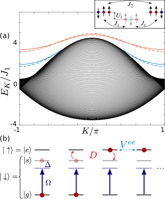
Figure 1: (a) Spectrum of two spin (Rydberg) excitations in a lattice versus the center of mass quasi-momentum $K$. The scattering states form a continuum spectrum (black), Eq. (5). The bound states for strong (red lines) and weak (blue lines) repulsive interactions are obtained from the spin-lattice Hamiltonian (dashed lines), Eq. (7), and from exact diagonalization of the Hamiltonian for the system sketched in (b) (solid lines). In the simulations, we used a lattice of size $L=100$ and periodic boundary conditions, with the spin model parameters $J_{2}/J_{1}=1/8$, $U_{1}/J_{1}=3.4,1.9$ for the red and blue dashed lines, respectively. Inset illustrates the motion of the bound pair via resonant two-site hopping $J_{2}$ and second order hopping $J_{1}^{2}/U_{1}$. (b) Level scheme of atoms to realize a spin-lattice model. Atoms in Rydberg states $\ket{e}$ and $\ket{s}$ undergo dipole-dipole exchange interaction $\ket{es}\to\ket{se}$ with rate $D$. The atomic ground state $\ket{g}$ is dressed with the Rydberg state $\ket{s}$ by a non-resonant laser with Rabi frequency $\Omega$ and detuning $\Delta\gg\Omega$. The spin-up and spin-down states correspond to $\ket{\uparrow}=\ket{e}$ and $\ket{\downarrow}\simeq\ket{g}+\frac{\Omega}{\Delta}\ket{s}$. Interactions $V^{ee}$ between the atoms in state $\ket{e}$ lead to formation of mobile bound states of Rydberg excitations. The parameters in numerical simulations shown in (a) correspond to $\Delta/\Omega=10$, $D_{1}/\Omega=1$, $V^{es}_{1}/\Omega=-0.125$, and $V^{ee}_{1}/\Omega=0.03,0.015$ for the red and blue solid lines, respectively.

Interacting spin excitations in a lattice.

We consider a spin lattice model described by Hamiltonian ($\hbar=1$)

$$\mathcal{H}=\sum_{i<j}J_{ij}\left(\hat{\sigma}^{+}_{i}\hat{\sigma}^{-}_{j}+\hat{\sigma}^{-}_{i}\hat{\sigma}^{+}_{j}\right)+\sum_{i<j}U_{ij}\hat{n}_{i}\hat{n}_{j},$$ (1)

where $\hat{\sigma}_{i}^{+}=\ket{\uparrow}_{i}\bra{\downarrow}$ and $\hat{\sigma}_{i}^{-}=\ket{\downarrow}_{i}\bra{\uparrow}$ are the raising and lowering operators for the spin at position $i$, and $\hat{n}_{i}\equiv\hat{\sigma}_{i}^{+}\hat{\sigma}_{i}^{-}=\ket{\uparrow}_{i}\bra{\uparrow}$ is the projector onto the spin-up state. In Eq. (1), the first term is responsible for the spin transport via the exchange interaction $J_{ij}$, while the second term describes the interaction between the spins in state $\ket{\uparrow}$ with strength $U_{ij}$. Both $J_{ij}$ and $U_{ij}$ have finite range and depend only on the distance $r=|i-j|$ between the spins at positions $i$ and $j$.

Hamiltonian (1) preserves the number of spin excitations. For a single excitation, the interaction does not play a role, and the Hamiltonian reduces to $\mathcal{H}^{(1)}_{J}=\sum_{x=1}^{L}\sum_{d\geq 1}J_{d}(\ket{x}\bra{x+d}+\ket{x}\bra{x-d})$, where $\ket{x}\equiv\hat{\sigma}^{+}_{x}\ket{\downarrow_{1}\downarrow_{2}\ldots\downarrow_{L}}$ denotes the state with the spin-up at position $x$ in a lattice of $L\gg 1$ spins (we assume periodic boundary conditions), and $d=1,2,\ldots$ is the range of the exchange interaction. The transformation $\ket{x}=\frac{1}{\sqrt{L}}\sum_{q}e^{iqx}\ket{q}$ diagonalizes the Hamiltonian, $\mathcal{H}^{(1)}_{J}=\sum_{q}\ket{q}\bra{q}E^{(1)}_{q}$, which indicates that the plane waves $\ket{q}=\frac{1}{\sqrt{L}}\sum_{x}e^{iqx}\ket{x}$ with the lattice quasi-momenta $q=\frac{2\pi\nu}{L}$ ($\nu=-\frac{L-1}{2},\ldots,\frac{L-1}{2}$) are the eigenstates of $\mathcal{H}^{(1)}_{J}$ with the eigenenergies $E^{(1)}_{q}=\sum_{d\geq 1}2J_{d}\cos(qd)$.

Consider now two spin excitations. We denote by $\ket{x,y}$ the state with one spin-up at position $x$ and the second spin-up at $y>x$. With this notation, the transport and interaction terms of the Hamiltonian (1) are given by

$$\mathcal{H}^{(2)}_{J}=\sum_{x<y} \Big{[}\sum_{d}\,J_{d}(\ket{x,y}\bra{x-d,y}+\ket{x,y}\bra{x,y+d})$$

$$+ \sum_{d<y-x}\!\!J_{d}(\ket{x,y}\bra{x+d,y}+\ket{x,y}\bra{x,y-d})$$

$$+ \sum_{d>y-x}\!\!J_{d}(\ket{x,y}\bra{y,x+d}+\ket{x,y}\bra{y-d,x})\Big{]},$$ (2)

$$\mathcal{H}^{(2)}_{U}=\sum_{x<y}U_{xy}\ket{x,y}\bra{x,y}.$$ (3)

We introduce the center of mass $R\equiv(x+y)/2$ and relative $r\equiv y-x$ coordinates. Making the transformation $\ket{R}=\frac{1}{\sqrt{\tilde{L}}}\sum_{K}e^{iKR}\ket{K}$ ($\tilde{L}=2L-3$), we obtain the total Hamiltonian $\mathcal{H}^{(2)}=\mathcal{H}^{(2)}_{J}+\mathcal{H}^{(2)}_{U}$ that is diagonal in the basis $\ket{K}$ of the center of mass quasi-momentum $K=\frac{2\pi\nu}{\tilde{L}}$: $\mathcal{H}^{(2)}=\sum_{K}\ket{K}\bra{K}\otimes\mathcal{H}_{K}$, where

$$\mathcal{H}_{K}=\sum_{r} \Big{[}\sum_{d}J_{d,K}\ket{r}\bra{r+d}+\sum_{d<r}J_{d,K}\ket{r}\bra{r-d}$$

$$+\sum_{d>r}J_{d,K}\ket{r}\bra{d-r}+U_{r}\ket{r}\bra{r}\Big{]},$$ (4)

with $J_{d,K}\equiv 2J_{d}\cos(Kd/2)$ SM . The two-body wavefunction can be cast as $\ket{\Psi(x,y)}=\frac{1}{\sqrt{\tilde{L}}}\sum_{K}e^{iKR}\ket{K}\otimes\sum_{r\geq 1}\psi_{K}(r)\ket{r}$, where the relative coordinate wavefunction $\psi_{K}(r)$ depends on the quasi-momentum $K$ as a parameter via the effective hopping rates $J_{d,K}$ in $\mathcal{H}_{K}$. There are two kinds of solutions of the eigenvalue problem $\mathcal{H}_{K}\ket{\psi_{K}}=E_{K}\ket{\psi_{K}}$ for $\ket{\psi_{K}}=\sum_{r\geq 1}\psi_{K}(r)\ket{r}$, corresponding to scattering states of asymptotically free magnons and to the interaction-bound states.

The wavefunction for the scattering states has the standard form containing the incoming and scattered plane waves $\psi_{K,k}(r>d_{U})=e^{ikr}+e^{-2i\delta_{K,k}}e^{-ikr}$, where $d_{U}$ is the (finite) range of the interaction potential $U_{r}$, and the phase shift $\delta_{K,k}$ depends on $U_{r}$. The energies of the scattering states are simply given by the sum of energies of two free magnons,

$$E_{K,k}^{(\mathrm{s})}=E^{(1)}_{q_{1}}+E^{(1)}_{q_{2}}=\sum_{d}2J_{d,K}\cos(kd),$$ (5)

where $K=q_{1}+q_{2}$ and $k=(q_{1}-q_{2})/2$ are the center of mass and relative quasi-momenta. In Fig. 1(a) we show the spectrum of the scattering states, assuming the range of the spin-exchange interaction $d_{J}=2$ with $J_{1}>J_{2}$, while $J_{d\geq 3}=0$. Note that due to the longer range hopping $J_{2}$, the spectrum at $K=\pm\pi$ does not reduce to a single point $E^{(\mathrm{s})}=0$ as in Valiente and Petrosyan (2008, 2009), but has a finite width $E_{K=\pi,k}^{(\mathrm{s})}\in[-4J_{2},4J_{2}]$, see also Piil and Mølmer (2007).

The bound state solutions correspond to a normalizable relative coordinate wavefunction, $\sum_{r}|\psi_{K}(r)|^{2}=1$. We assume nearest-neighbor interaction, $U_{1}\neq 0$ and $U_{r>1}=0$ in Eq. (4). We set $\psi_{K}(0)=0$ and $\psi_{K}(1)=c$, with $c$ some constant, and make the ansatz

$$\psi_{K}(r)=\alpha_{K}\psi_{K}(r-1)+\beta_{K}\psi_{K}(r-2).$$ (6)

The physical intuition behind this recurrence relation is that every (discrete) position $r$ can be reached from positions $r-1$ and $r-2$ with the amplitudes $\alpha_{K}\propto J_{1}$ and $\beta_{K}\propto J_{2}$. We then obtain SM $\alpha_{K}=\frac{J_{1,K}}{U_{1}}$, $\beta_{K}=\frac{J_{2,K}}{U_{1}+J_{2,K}}$, and the energy of the bound state

$$E_{K}^{(\mathrm{b})}= 2J_{2,K}+\frac{J_{1,K}^{2}}{U_{1}}+\frac{J_{1,K}^{2}J_{2,K}}{U_{1}^{2}}+\frac{U_{1}^{2}}{U_{1}+J_{2,K}}.$$ (7)

The first term on the right-hand-side of this equation does not depend on the interaction $U_{1}$ and it describes two-site resonant hopping of the excitation over the other excitation, $\ket{x-1,x}\leftrightarrow\ket{x,x+1}$, with rate $\propto J_{2}$. This process is resonant because the relative distance $r=1$, and thereby the interaction energy, are conserved during this two-excitation “somersault”. The second and third terms are contributions from the second-order ($\propto J_{1}^{2}/U_{1}$) and third-order ($\propto J_{1}^{2}J_{2}/U_{1}^{2}$) hopping processes. The last term is the energy shift due to interaction $U_{1}$.

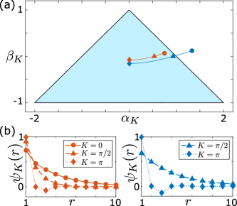
Figure 2: (a) Diagram of values of $\alpha_{K}$, $\beta_{K}$ for the existence of bound states (light-blue shaded region). (b) Wavefunction $\psi_{K}(r)$ versus the relative distance $r$ for several values of the center of mass quasi-momentum $K$. The parameters are the same as in Fig. 1, with $U_{1}/J_{1}=3.4$ (left graph and red line in (a)), and $U_{1}/J_{1}=1.9$ (right graph and blue line in (a)) where the bound state does not exist in the vicinity of $K=0$.

The above solution is valid under the conditions that bound-state wavefunction is normalizable. Inserting $\psi_{K}(r)\propto\lambda^{r}$ into Eq. (6), we obtain that the wavefunction exponentially decays with distance $r$, and therefore is normalizable, when $\mbox{$\frac{1}{2}$}|\alpha_{K}\pm\sqrt{\alpha_{K}^{2}+4\beta_{K}^{2}}|<1$. In Fig. 2(a) we show the values of $\alpha_{K}$ and $\beta_{K}$, forming a triangular region, for which there exists an exponentially localized bound state. With only nearest-neighbor hopping ($J_{2}=0$), we recover the condition $|\alpha_{K}|<1$ of Refs. Valiente and Petrosyan (2008, 2009). For a given set of parameters $J_{1},J_{2},U_{1}$, the bound state may not exists for all values of the center of mass quasi-momentum $K$, since both $\alpha_{K}$ and $\beta_{K}$ depend on $K$. In general, the closer is the point ($\alpha_{K},\beta_{K}$) to the boundary of the shaded region in Fig. 2(a), the less localized is the bound state wavefunction, as we illustrate with two examples in Fig. 2(b). In Fig. 3 we show the diagrams of $J_{2}/J_{1}$ and $U_{1}/J_{1}$ versus $K$ for the existence of the bound states. Clearly, for certain sets of parameters, the bound states do not exist at all, or exist only within a certain interval of values of $K$.

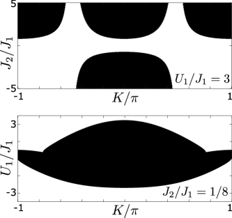
Figure 3: Diagram of values of $J_{2}/J_{1}$, for fixed $U_{1}=3J_{1}$ (upper panel), and $U_{1}/J_{1}$, for fixed $J_{2}=J_{1}/8$ (lower panel), versus $K$, for the existence (white regions) and absence (black regions) of the bound states.

Rydberg dressed atoms in a lattice.

The spin lattice model of Eq. (1) might be realized with a regular array of atoms in Rydberg states $\ket{s}$ and $\ket{e}$. We could excite one or more atoms to state $\ket{e}=\ket{\uparrow}$ and prepare all the remaining atoms in state $\ket{s}=\ket{\downarrow}$. Assuming the transition $\ket{s}\leftrightarrow\ket{e}$ is dipole allowed, resonant dipole-dipole interaction between the atoms separated by $d$ lattice sites would lead to transfer of excitations via the exchange interaction $\ket{es}\leftrightarrow\ket{se}$ with rate $D_{d}=\frac{C_{3}/a^{3}}{d^{3}}$, where $C_{3}$ is the interaction coefficient and $a$ is the lattice constant Barredo et al. (2015); de Léséleuc et al. (2017). Atoms in the Rydberg states also interact via the van der Waals interactions $V^{\mu\nu}_{d}=\frac{C_{6}^{\mu\nu}/a^{6}}{d^{6}}$, which would map onto the interactions $U$ between the spin excitations Schauß et al. (2012, 2015); Labuhn et al. (2016); Lienhard et al. (2017); Bernien et al. (2017), provided $V^{ee}$ differs from the interaction $V^{es}$ between the $\ket{e}$ and $\ket{s}$ state atoms.

Typically, however, the resonant dipole-dipole interaction $D$ is orders of magnitude stronger than the van der Waals interactions $V$, since the latter originate from non-resonant dipole-dipole interactions, $V\sim D^{2}/\delta\omega$, with large Förster defects, $\delta\omega\gg D$ Saffman et al. (2010). Small interactions $V\ll D$ will preclude the interplay between the spin transport and spin-spin interactions. To mitigate this problem, we propose to dress trapped ground state atoms with the Rydberg state $\ket{s}$. The dressing laser would then mediate hopping of the Rydberg excitation $\ket{e}$ to nearby atoms in the dressed ground state with rates $J_{d}$ which can be made comparable to, or even weaker than, the effective interaction $U_{r}$ between the excitations. Rydberg dressing of ground-state atoms Bouchoule and Mølmer (2002); Henkel et al. (2010); Johnson and Rolston (2010); Pupillo et al. (2010); Wüster et al. (2011); Macrì and Pohl (2014) is a versatile tool for tuning interatomic interactions to simulate various lattice models Schempp et al. (2015); Glaetzle et al. (2015); van Bijnen and Pohl (2015); Buchmann et al. (2017); Zeiher et al. (2016, 2017).

We consider an array of single atoms with the level scheme shown in Fig. 1(b). The ground state $\ket{g}$ of each atom is coupled to the Rydberg state $\ket{s}$ by a laser with Rabi frequency $\Omega$ and large detuning $\Delta\gg\Omega$. We assume that $\Delta$ is much larger than the resonant dipole-dipole interactions $D_{d}$ between the $\ket{s}$ and $\ket{e}$ state atoms separated by $d=1,2,\ldots$ lattice sites. The van der Waals interactions $V^{\mu\nu}_{r}$ are assumed to be still weaker, so the hierarchy of the energy scales is $\Delta\gg\Omega,D_{d}\gtrsim V^{ee}_{r},V^{es}_{r},V^{ss}_{r}$.

The laser instills a small admixture $\frac{\Omega}{\Delta}\ket{s}$ of the Rydberg state to the ground state $\ket{g}$ SM . We then identify the dressed ground state with the spin-down state, $\ket{\downarrow}\simeq\ket{g}+\frac{\Omega}{\Delta}\ket{s}$, while the spin-up state is $\ket{\uparrow}=\ket{e}$. Neglecting the interactions $\sim\frac{\Omega^{4}}{\Delta^{4}}V^{ss}_{r}$ between the dressed ground state atoms, we adiabatically eliminate the nonresonant state $\ket{s}$ and obtain effective excitation hopping rates $J_{d}\simeq\frac{\Omega^{2}D_{d}}{\Delta^{2}}$ between the atoms separated by $d$ lattice sites. Since $D_{d}\propto d^{-3}$, we can truncate $J_{d}$ to range $d_{J}=2$. More careful considerations show that the hopping rates $J_{1,2}$ for a Rydberg excitation are slightly altered when another Rydberg excitation is in a close proximity SM . We assume that the lifetime of the Rydberg state $\ket{e}$ is longer than the timescale $J_{d}^{-1}$ for the system dynamics and neglect dissipation. The number of atoms prepared in state $\ket{e}$ is then conserved. Decay via the non-resonant state $\ket{s}$ is suppressed by the factor of $\frac{\Omega^{2}}{\Delta^{2}}$.

For the effective interaction potential between the excitations we obtain $U_{r}\simeq V^{ee}_{r}+2\frac{\Omega^{2}D_{r}^{2}}{\Delta^{3}}$, where both terms scale with distance as $\propto r^{-6}$. We assume that $U_{r}$ is dominated by the nearest-neighbor van der Waals interaction $V^{ee}_{1}$ between the atoms in Rydberg states $\ket{e}$. Corrections to the level shift of Rydberg dressed atoms in the vicinity of the Rydberg excited atom $\ket{e}$ lead to small contribution to $U_{r}$ and weak longer range interaction SM . Despite these small variations of $J_{d}(r)$ and $U_{r}$ with distance $r$ between Rydberg excitations, the spin-lattice model approximates well the properties of interacting Rydberg excitations, including the two-excitation bound states shown in Fig. 1(a).

The dynamics of Rydberg excitations in a lattice and their bound states can be prepared and observed with the presently available experimental techniques. We envisage an array of single atoms confined in a chain of microtraps Barredo et al. (2016); Endres et al. (2016). Using focused laser beams, selected atoms can be resonantly excited from the ground state $\ket{g}$ to the Rydberg state $\ket{e}$, while the dressing laser is turned off, $\Omega=0$. Next, turning on the dressing laser, $\Omega\neq 0$ will lead to the admixture of the Rydberg state $\ket{s}$ to the ground state atoms, which will induce the $\ket{e}$ excitation hopping between the atoms due the dipole-dipole exchange interaction. With realistic experimental parameters SM , hopping rates $J_{1}\simeq 200\>$kHz and $J_{2}=J_{1}/8$ can be achieved. This will allow observation of non-trivial dynamics of the excitations on the timescale of Rydberg state lifetimes $\tau\gtrsim 100\>\mu$s. With a proper choice of state $\ket{e}$, we can ensure appropriate interaction strength $U_{1}\simeq V^{ee}\gtrsim J_{1}$, which will result in the formation of tightly bound Rydberg excitations that are still mobile as they propagate with rate $\sim J_{2}$. Free Rydberg excitations and their scattering states can be discriminated from the interaction-bound states spectroscopically or by the fast and slow dynamics, respectively. Turning off the dressing laser would freeze the dynamics and individual Rydberg excitations can be detected with high efficiency and single-site resolution Labuhn et al. (2016); Bernien et al. (2017); Lienhard et al. (2017).

Conclusions.

We have shown that spin lattice models with controllable long range hopping and interactions between the spin excitations can be realized with Rydberg dressed atoms in a lattice. We have found mobile bound states of spin excitations which are quantum lattice solitons. It would be interesting to consider bound aggregates of more than two magnons which may form mobile clusters that can propagate via resonant long-range hopping process. In turn, multiple clusters can form a lattice liquid Mattioli et al. (2013); Dalmonte et al. (2015), while including controllable dephasing and disorder Schempp et al. (2015); Schönleber et al. (2015) may change the transport of (bound) Rydberg excitations from ballistic to diffusive or localized. Hence, this system can be used to simulate and study few- and many-body quantum dynamics in spin lattices.

I Supplemental Material

I.1 Details of derivation of the two-excitation wavefunction in a spin lattice

Consider two spin excitations in a lattice. The transport and interaction Hamiltonians are given by Eqs. (Interacting spin excitations in a lattice.) and (3) in the main text, namely

$$\mathcal{H}^{(2)}_{J}=\sum_{x<y} \Big{[}\sum_{d}\,J_{d}(\ket{x,y}\bra{x-d,y}+\ket{x,y}\bra{x,y+d})$$

$$+ \sum_{d<y-x}\!\!J_{d}(\ket{x,y}\bra{x+d,y}+\ket{x,y}\bra{x,y-d})$$

$$+ \sum_{d>y-x}\!\!J_{d}(\ket{x,y}\bra{y,x+d}+\ket{x,y}\bra{y-d,x})\Big{]},$$ (8)

and

$$\mathcal{H}^{(2)}_{U}=\sum_{x<y}U_{xy}\ket{x,y}\bra{x,y},$$ (9)

where $\ket{x,y}$ denotes the state with the excited spins at positions $x$ and $y>x$.

We introduce the center of mass $R\equiv(x+y)/2$ and relative $r\equiv y-x$ coordinates: $R=1+\mbox{$\frac{1}{2}$},2,2+\mbox{$\frac{1}{2}$},\ldots,L-\mbox{$\frac{1}{2}$}$ takes $\tilde{L}=2L-3$ discrete values, and $r=1,2,\ldots,L-1$ takes $L-1$ values. In terms of these coordinates, the transport Hamiltonian reads

$$\mathcal{H}^{(2)}_{J}=\sum_{R,r} \Big{[}\sum_{d}J_{d}(\ket{R}\bra{R-d/2}\otimes\ket{r}\bra{r+d}+\ket{R}\bra{R+d/2}\otimes\ket{r}\bra{r+d})$$

$$+ \;\sum_{d<r}J_{d}(\ket{R}\bra{R+d/2}\otimes\ket{r}\bra{r-d}+\ket{R}\bra{R-d/2}\otimes\ket{r}\bra{r-d})$$

$$+ \;\sum_{d>r}J_{d}(\ket{R}\bra{R+d/2}\otimes\ket{r}\bra{d-r}+\ket{R}\bra{R-d/2}\otimes\ket{r}\bra{d-r})\Big{]},$$ (10)

Similarly to the single excitation case, we can diagonalize the center of mass part of $\mathcal{H}^{(2)}_{J}$ by the transformation $\ket{R}=\frac{1}{\sqrt{\tilde{L}}}\sum_{K}e^{iKR}\ket{K}$, where $K=\frac{2\pi\nu}{\tilde{L}}$ ($\nu=-\frac{\tilde{L}-1}{2},\ldots,\frac{\tilde{L}-1}{2}$) is the center of mass quasi-momentum:

$$\mathcal{H}^{(2)}_{J}=\sum_{K}\ket{K}\bra{K}\otimes\sum_{r} \Big{[}\sum_{d}J_{d,K}\ket{r}\bra{r+d}$$

$$+ \;\sum_{d<r}J_{d,K}\ket{r}\bra{r-d}$$

$$+ \;\sum_{d>r}J_{d,K}\ket{r}\bra{d-r}\Big{]},$$ (11)

where $J_{d,K}\equiv 2J_{d}\cos(Kd/2)$. The interaction Hamiltonian remains diagonal in these coordinates,

$$\mathcal{H}^{(2)}_{U}=\sum_{K}\ket{K}\bra{K}\otimes\sum_{r}U_{r}\ket{r}\bra{r},$$ (12)

and the total Hamiltonian can be cast as

$$\mathcal{H}^{(2)}=\mathcal{H}^{(2)}_{J}+\mathcal{H}^{(2)}_{U}=\sum_{K}\ket{K}\bra{K}\otimes\mathcal{H}_{K}.$$

We have thus reduced the two-body problem for

$$\ket{\Psi(x,y)} =\sum_{x<y}\Psi(x,y)\ket{x,y}$$

$$=\frac{1}{\sqrt{\tilde{L}}}\sum_{K}e^{iKR}\ket{K}\otimes\sum_{r\geq 1}\psi_{K}(r)\ket{r}$$ (13)

to a one-body problem for the relative coordinate wavefunction $\psi_{K}(r)$, which depends on the center of mass quasi-momentum $K$ as a parameter via the effective hopping rates $J_{d,K}$ in $\mathcal{H}_{K}$.

Our aim is to solve the eigenvalue problem

$$\mathcal{H}_{K}\ket{\psi_{K}}=E_{K}\ket{\psi_{K}}$$ (14)

for the relative coordinate wavefunction $\ket{\psi_{K}}=\sum_{r\geq 1}\psi_{K}(r)\ket{r}$. The scattering solutions are expressed via the plane waves as given in the main text. We present here the details of derivation of the bound solutions corresponding to a normalizable [localized] relative coordinate wavefunction, $\sum_{r}|\psi_{K}(r)|^{2}=1$ [with $\psi_{K}(r\to\infty)\to 0$].

We assume range $d_{U}=1$ (nearest-neighbor) interaction, $U_{1}\neq 0$ and $U_{r>1}=0$ in Eq. (12), leading to the Hamiltonian

$$\mathcal{H}_{K}=\sum_{r\geq 1} \Big{[}J_{1,K}(\ket{r}\bra{r+1}+\ket{r+1}\bra{r})$$

$$+ \;J_{2,K}(\ket{r}\bra{r+2}+\ket{r+2}\bra{r})\Big{]}$$

$$+(U_{1}+J_{2,K})\ket{1}\bra{1}.$$ (15)

This results in the equation

$$J_{1,K}\big{[}\psi_{K}(r+1)+\psi_{K}(r-1)\big{]}$$

$$+ J_{2,K}\big{[}\psi_{K}(r+2)+\psi_{K}(r-2)\big{]}$$

$$+ (U_{1}+J_{2,K})\delta_{r,1}\psi_{K}(r)=E_{K}\psi_{K}(r).$$ (16)

We set $\psi_{K}(0)=0$ and $\psi_{K}(1)=c$, with $c$ some constant to be determined by the normalization. We make an ansatz for the wavefunction,

$$\psi_{K}(r)=\alpha_{K}\psi_{K}(r-1)+\beta_{K}\psi_{K}(r-2).$$ (17)

The physical meaning of this recurrence relation is that every site $r$ can be reached from the previous two sites $r-1$ and $r-2$ with the amplitudes $\alpha_{K}\propto J_{1}$ and $\beta_{K}\propto J_{2}$. Starting from position $r=1$, the wavefunction at any $r$ can then be written as

$$\psi_{K}(r)=c\sum_{n=0}^{\lfloor(r-1)/2\rfloor}{{r-1-2n}\choose{n}}\alpha_{K}^{r-1-2n}\beta_{K}^{n},$$ (18)

where $\lfloor\cdot\rfloor$ is the floor function, and the binomial coefficients count the weights for different path from site $1$ to $r>1$. For instance, we can reach $\ket{r=4}$ from $\ket{1}$ by three one-site hoppings $\propto\alpha_{K}^{3}$, or by two-site hopping $\beta_{K}$ followed by one-site hopping $\alpha_{K}$, or vice versa, $\propto\beta_{K}\alpha_{K}+\alpha_{K}\beta_{K}=2\alpha_{K}\beta_{K}$. Using the ansatz (18) in Eqs. (I.1) for $r=1,2,3$ we obtain a set of three equations,

$$E_{K}=(U_{1}+J_{2,K})+J_{1,K}\alpha_{K}+J_{2,K}(\alpha_{K}^{2}+\beta_{K}),$$ (19a)

$$E_{K}\alpha_{K}=J_{1,K}(\alpha_{K}^{2}+\beta_{K}+1)+J_{2,K}(\alpha_{K}^{3}+2\alpha_{K}\beta_{K}),$$ (19b)

$$E_{K}(\alpha_{K}^{2}+\beta_{K})=J_{1,K}(\alpha_{K}+\alpha_{K}^{3}+2\alpha_{K}\beta_{K})$$

$$\qquad\qquad\qquad\;\;+J_{2,K}(1+\alpha_{K}^{4}+3\alpha_{K}^{2}\beta_{K}+\beta_{K}^{2}),$$ (19c)

for the unknowns $\alpha_{K},\beta_{K},E_{K}$. Solving these equations, we obtain

$$\alpha_{K}=\frac{J_{1,K}}{U_{1}},\quad\beta_{K}=\frac{J_{2,K}}{U_{1}+J_{2,K}},$$ (20)

while the energy of the bound state is

$$E_{K}^{(\mathrm{b})}= 2J_{2,K}+\frac{J_{1,K}^{2}}{U_{1}}+\frac{J_{1,K}^{2}J_{2,K}}{U_{1}^{2}}+\frac{U_{1}^{2}}{U_{1}+J_{2,K}}.$$ (21)

The physical meanings of the various terms of this equation are discussed in the main text.

We finally discuss the conditions of validity of the above solution under which the bound-state wavefunction is normalizable, $\sum_{r}|\psi_{K}(r)|^{2}=1$. Assuming $\psi_{K}(r)\propto\lambda^{r}$ and inserting into Eq. (17), we obtain the quadratic equation $\lambda^{2}=\alpha_{K}\lambda+\beta_{K}$ with the solutions

$$\lambda_{1,2}=\frac{\alpha_{K}\pm\sqrt{\alpha_{K}^{2}+4\beta_{K}^{2}}}{2}.$$

We can now write the wavefunction as

$$\psi_{K}(r)=c_{1}\lambda_{1}^{r}+c_{2}\lambda_{2}^{r},$$ (22)

and determine the coefficients $c_{1,2}$ from $\psi_{K}(0)=0$ and $\psi_{K}(1)=c$, leading to $c_{2}=-c_{1}=\frac{c}{\sqrt{\alpha_{K}^{2}+4\beta_{K}^{2}}}$. This is of course the same wavefunction as in Eq. (18). More important, however, is that we have found that $\psi_{K}(r)\propto\lambda_{1,2}^{r}$ exponentially decays with distance $r$, and therefore is normalizable, when both $|\lambda_{1,2}|=\mbox{$\frac{1}{2}$}|\alpha_{K}\pm\sqrt{\alpha_{K}^{2}+4\beta_{K}^{2}}|<1$.

I.1.1 Truncation of interaction range

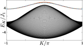
Figure 4: Scattering (black) and bound-state (red solid line) spectra obtained by exact numerical diagonalization of Hamiltonian with long range interactions $J_{d}=J_{1}/d^{3}$ and $U_{r}=U_{1}/r^{6}$ ($U_{1}/J_{1}=4$). The bound state energy $E_{K}$ of Eq. (21) (dashed blue line), obtained with truncated interactions ($d_{J}=2$ and $d_{U}=1$), is nearly indistinguishable from the exact result.

Our formalism to obtain the bound states of excitations in a lattice can be easily extended to longer range hopping $J_{d}$ and interaction $U_{r}$. We are, however, mainly concerned with the typical case of resonant dipole-dipole exchange interaction, leading to $J_{d}\propto 1/d^{3}$, and van der Waals repulsive or attractive interaction, leading to $U_{r}\propto 1/r^{6}$. We have therefore truncated $J_{d}$ to range $d_{J}=2$ and $U_{r}$ to range $d_{U}=1$. In Fig. 4 we show the spectra for the scattering and bound states obtained without the truncation. This figure clearly demonstrates that the above approximations are well justified for the power-law decay of the strengths of $J_{d}$ and $U_{r}$ with distance.

I.2 Derivation of the effective excitation hopping rate and interaction strength for Rydberg dressed atoms in a lattice

Consider an ensemble of atoms in a lattice with period $a$, with one atom per site. A spatially uniform laser field of frequency $\omega$ couples the ground state $\ket{g}$ of each atom to the Rydberg state $\ket{s}$ with the Rabi frequency $\Omega$ and detuning $\Delta=\omega_{sg}-\omega$, see Fig. 1(b) of the main text. Resonant dipole-dipole interaction between the atoms at positions $i$ and $j$ leads to the exchange interaction $\ket{es}\leftrightarrow\ket{se}$ with rate $D_{ij}=\frac{C_{3}/a^{3}}{|i-j|^{3}}$, where $C_{3}$ is the interaction coefficient. Including also the van der Waals interactions $V^{\mu\nu}_{ij}=\frac{C_{6}^{\mu\nu}/a^{6}}{|i-j|^{6}}$ between the Rydberg states, the Hamiltonian in the rotating frame reads ($\hbar=1$)

$$\mathcal{H}_{\mathrm{at}}= \sum_{j}\left[\Delta\hat{\sigma}^{ss}_{j}-\Omega\left(\hat{\sigma}^{gs}_{j}+\hat{\sigma}^{sg}_{j}\right)\right]$$

$$+\sum_{i<j}D_{ij}\left(\hat{\sigma}^{es}_{i}\hat{\sigma}^{se}_{j}+\hat{\sigma}^{se}_{i}\hat{\sigma}^{es}_{j}\right)$$

$$+\sum_{i<j}\left(V^{ee}_{ij}\hat{\sigma}^{ee}_{i}\hat{\sigma}^{ee}_{j}+V^{ss}_{ij}\hat{\sigma}^{ss}_{i}\hat{\sigma}^{ss}_{j}+V^{es}_{ij}\hat{\sigma}^{ee}_{i}\hat{\sigma}^{ss}_{j}\right),$$ (23)

where $\hat{\sigma}^{\mu\nu}_{j}=\ket{\mu}_{j}\bra{\nu}$ are the atomic operators.

We take the detuning $\Delta$ of the laser field to be much larger than the Rabi frequency $\Omega$ as well as the resonant dipole-dipole interactions $D_{d}=\frac{C_{3}/a^{3}}{d^{3}}$ between the Rydberg-state atoms separated by $d=1,2,\ldots$ lattice sites. The van der Waals interactions $V^{\mu\nu}_{d}=\frac{C_{6}^{\mu\nu}/a^{6}}{d^{6}}$ are assumed to be still weaker, $\Delta\gg\Omega,D_{d}>V^{ee}_{d},V^{es}_{d},V^{ss}_{d}$.

I.2.1 Rydberg dressing

For a single (isolated) atom, the dipole-dipole and van der Waals interactions are irrelevant, and the Hamiltonian reduces to that for a two level system,

$$\mathcal{H}_{\mathrm{TLS}}=\Delta\ket{s}\bra{s}-\Omega(\ket{g}\bra{s}+\ket{s}\bra{s}).$$ (24)

[We set the energy of the ground state $\ket{g}$ to zero and work in a rotating frame in which the energy of state $\ket{e}$ is also zero]. The eigenstates and corresponding eigenvalues of this Hamiltonian are

$$\ket{\pm}=\frac{\varepsilon_{\mp}\ket{g}+\Omega\ket{s}}{\sqrt{\varepsilon_{\mp}^{2}+\Omega^{2}}},\quad\varepsilon_{\pm}=\frac{\Delta\pm\sqrt{\Delta^{2}+4\Omega^{2}}}{2}.$$ (25)

For $\Delta\gg\Omega$, the eigenstate $\ket{-}\simeq\ket{g}+\frac{\Omega}{\Delta}\ket{s}$, with shifted energy $\varepsilon_{-}\simeq-\frac{\Omega^{2}}{\Delta}\equiv\delta$ (ac Stark shift), corresponds to the ground state $\ket{g}$ with a small admixture of the Rydberg state $\ket{s}$. We identify this Rydberg dressed ground state with the spin-down state, $\ket{\downarrow}\equiv\ket{-}$, while the spin-up state is $\ket{\uparrow}\equiv\ket{e}$.

A pair of dressed ground-state atoms would interact with each other via the Rydberg state $\ket{s}$ components. Each atom is in state $\ket{s}$ with probability $\frac{\Omega^{2}}{\Delta^{2}}$ and therefore the two-atom interaction strength is $\frac{\Omega^{4}}{\Delta^{4}}V^{ss}_{r}$ Buchmann et al. (2017). We neglect this weak interaction and instead focus below on the interatomic interactions that are up to second order in $\frac{\Omega}{\Delta}$. Hence, with $L$ atoms in a lattice, all in the dressed ground state, the total energy shift is

$$E_{0}=\sum_{i}^{L}\delta_{i}=-L\frac{\Omega^{2}}{\Delta}.$$ (26)

This constant energy shift can be disregarded by redefining the zero-point energy, e.g., by absorbing the ac Stark shift into the laser detuning, $\omega\to\omega+\frac{\Omega^{2}}{\Delta}$.

I.2.2 Single excitation

Assume now that one atom is excited to state $\ket{e}$ while the rest of the atoms are in the dressed ground state. Our aim is to derive the effective hopping rate of the single Rydberg excitation in the lattice and the modification of the ac Stark shifts of the ground state atoms in the vicinity of the excited one. We are interested in the interatomic interactions that are up to second order in $\frac{\Omega}{\Delta}$, which thus involve no more that one (virtual) $\ket{s}$ excitation. It is therefore sufficient to consider the two atom state

$$\ket{\phi}=c_{ge}\ket{ge}+c_{eg}\ket{eg}+c_{se}\ket{se}+c_{es}\ket{es}$$ (27)

and the corresponding Hamiltonian

$$\mathcal{H}^{(1)}_{\mathrm{at}}= \Delta_{y}^{(x)}\ket{se}\bra{se}+\Delta_{x}^{(y)}\ket{es}\bra{es}$$

$$-\Omega(\ket{ge}\bra{se}+\ket{eg}\bra{es}+\mathrm{H.c.})$$

$$+D_{xy}(\ket{se}\bra{es}+\mathrm{H.c.}),$$ (28)

where $x$ and $y$ denote the positions of the two atoms, and we defined $\Delta_{y}^{(x)}\equiv\Delta+V^{se}_{xy}=\Delta_{x}^{(y)}$. The equations for the amplitudes $c_{\nu\mu}$ of the state vector $\ket{\phi}$ are then

$$i\dot{c}_{ge} =-\Omega c_{se},$$ (29a)

$$i\dot{c}_{eg} =-\Omega c_{es},$$ (29b)

$$i\dot{c}_{se} =(\Delta+V^{se}_{xy})c_{se}-\Omega c_{ge}+D_{xy}c_{es},$$ (29c)

$$i\dot{c}_{es} =(\Delta+V^{se}_{xy})c_{es}-\Omega c_{eg}+D_{xy}c_{se}.$$ (29d)

We adiabatically eliminate states containing the highly detuned Rydberg state $\ket{s}$. To that end, we set $\dot{c}_{se}=0$ and $\dot{c}_{es}=0$ and solve the last two equations for ${c}_{se}$ and ${c}_{es}$. Inserting the solution into the first two equations, we obtain

$$i\dot{c}_{ge} =-\frac{\Omega^{2}(\Delta+V^{se}_{xy})}{(\Delta+V^{se}_{xy})^{2}-D_{xy}^{2}}c_{ge}+\frac{\Omega^{2}D_{xy}}{(\Delta+V^{se}_{xy})^{2}-D_{xy}^{2}}c_{eg},$$ (30a)

$$i\dot{c}_{eg} =-\frac{\Omega^{2}(\Delta+V^{se}_{xy})}{(\Delta+V^{se}_{xy})^{2}-D_{xy}^{2}}c_{eg}+\frac{\Omega^{2}D_{xy}}{(\Delta+V^{se}_{xy})^{2}-D_{xy}^{2}}c_{ge}.$$ (30b)

We can interpret these equations as follows: The dressed $\ket{g}$ state atom at position $y$ acquires an energy shift

$$\delta_{y}^{(x)}=-\frac{\Omega^{2}(\Delta+V^{se}_{xy})}{(\Delta+V^{se}_{xy})^{2}-D_{xy}^{2}},$$ (31)

which depends on the position $x$ of the $\ket{e}$ excitation. Besides, states $\ket{eg}$ and $\ket{ge}$ are coupled via exchange interaction

$$J_{xy}=\frac{\Omega^{2}D_{xy}}{(\Delta+V^{se}_{xy})^{2}-D_{xy}^{2}}.$$ (32)

This effective excitation hopping rate $J_{xy}=J_{d}$ depends on the relative distance $d=|x-y|$.

Hence, the total energy of $L$ atoms in a lattice with a single $\ket{e}$ excitation is

$$E_{1}=\sum_{y\neq x}\delta_{y}^{(x)}.$$ (33)

This sum has now $L-1$ terms. The terms $\delta_{y}^{(x)}$ with small separation $|x-y|\geq 1$ are affected by the $D_{xy}$ and $V^{se}_{xy}$ interactions, while the terms with $|x-y|\gg 1$ are obviously equal to the ac Stark shift $\delta=-\frac{\Omega^{2}}{\Delta}$ of a non-interacting atom. Due to the translational invariance of the lattice, $E_{1}$ does not depend on the position $x$ of the $\ket{e}$ excitation. $E_{1}$ is therefore a constant which can be disregarded by redefining the zero-point energy [notice, however, that $E_{1}\neq E_{0}$].

We thus obtain an effective Hamiltonian for a single excitation hopping on a lattice,

$$\mathcal{H}^{(1)}_{J} =\sum_{x\neq y}J_{xy}\ket{x}\bra{y}$$

$$=\sum_{x=1}^{L}\sum_{d\geq 1}J_{d}(\ket{x}\bra{x+d}+\ket{x}\bra{x-d}),$$ (34)

which has the same form as $\mathcal{H}^{(1)}_{J}$ in the main text. For $\Delta\gg D_{d},V^{es}_{d}$, the excitation hopping rates

$$J_{d}\simeq\frac{\Omega^{2}D_{d}}{\Delta^{2}}\propto 1/d^{3}$$ (35)

can be truncated to range $d_{J}=2$.

I.2.3 Two excitations

Consider finally two $\ket{e}$ excitations in the lattice. As argued above, to determine interatomic interactions that are up to second order in $\frac{\Omega}{\Delta}$, we can restrict our analysis to the multiatom configurations with at most one atom in state $\ket{s}$. It is then sufficient to consider the three atom state

$$\ket{\phi}= \;c_{gee}\ket{gee}+c_{ege}\ket{ege}+c_{eeg}\ket{eeg}$$

$$+c_{see}\ket{see}+c_{ese}\ket{ese}+c_{ees}\ket{ees}.$$ (36)

We assume, as before, that the interaction $V^{ee}_{d}$ between the $\ket{e}$ excitations is weak, $V^{ee}_{d}\ll\Omega,D_{d}\ll\Delta$, and neglect it here; later we account for $V^{ee}_{d}$ exactly in the effective Hamiltonian. The three-atom Hamiltonian is

$$\mathcal{H}^{(2)}_{\mathrm{at}}= \Delta_{x,y}^{(z)}\ket{ees}\bra{ees}+\Delta_{x,z}^{(y)}\ket{ese}\bra{ese}+\Delta_{y,z}^{(x)}\ket{see}\bra{see}$$

$$-\Omega(\ket{gee}\bra{see}+\ket{ege}\bra{ese}+\ket{eeg}\bra{ees}+\mathrm{H.c.})$$

$$+D_{xy}(\ket{see}\bra{ese}+\mathrm{H.c.})$$

$$+D_{xz}(\ket{see}\bra{ees}+\mathrm{H.c.})$$

$$+D_{yz}(\ket{ese}\bra{ees}+\mathrm{H.c.}),$$ (37)

where $x,y,z$ denote the positions of the atoms, $\Delta_{x,y}^{(z)}\equiv\Delta+V^{se}_{xz}+V^{se}_{yz}$ and similarly for $\Delta_{x,z}^{(y)}$ and $\Delta_{y,z}^{(x)}$. From the differential equations for the amplitudes $c_{\lambda\mu\nu}$ of $\ket{\phi}$, we adiabatically eliminate the amplitudes corresponding to the highly-detuned $\ket{s}$ state, i.e., we set $\dot{c}_{ees}=\dot{c}_{ese}=\dot{c}_{see}=0$, solve for the amplitudes $c_{ees},c_{ese},c_{see}$ and insert them into the remaining equations. The resulting equations have the form

$$\dot{c}_{eeg}= \frac{\Omega^{2}(\Delta_{x,z}^{(y)}\Delta_{y,z}^{(x)}-D_{xy}^{2})}{\Gamma(x,y,z)}c_{eeg}$$

$$+\frac{\Omega^{2}(D_{xy}D_{xz}-D_{yz}\Delta_{y,z}^{(x)})}{\Gamma(x,y,z)}c_{ege}$$

$$+\frac{\Omega^{2}(D_{xy}D_{yz}-D_{yz}\Delta_{x,z}^{(y)})}{\Gamma(x,y,z)}c_{gee},$$ (38)

with $\Gamma(x,y,z)\equiv-\Delta_{x,y}^{(z)}\Delta_{x,z}^{(y)}\Delta_{y,z}^{(x)}-2D_{xy}D_{xz}D_{yz}+\Delta_{x,y}^{(z)}D_{xy}^{2}+\Delta_{x,z}^{(y)}D_{x,z}^{2}+\Delta_{y,z}^{(x)}D_{y,z}^{2}$, and similarly for $\dot{c}_{ege}$ and $\dot{c}_{gee}$. The first term in Eq. (I.2.3) corresponds to the energy shift of the dressed $\ket{g}$ state atom, while the other two terms describe the exchange interactions between the atom in state $\ket{g}$ and the atoms in state $\ket{e}$.

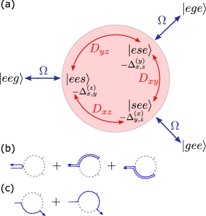
Figure 5: (a) Diagram of transitions for retrieving the perturbative energy shifts and excitation hopping rates for two excited $\ket{e}$ and one ground $\ket{g}$ state atoms. The atomic positions are $x,y,z$. Red-shaded region denotes the high energy subspace, $\Delta\gg\Omega,D$, which is eliminated adiabatically. (b) Illustration of three virtual processes contributing to the energy shift of $\ket{eeg}$, as per Eq. (39). (c) Two possible paths for the hopping process $\ket{eeg}\leftrightarrow\ket{gee}$ given by Eq. (40).

Using series expansion in $\frac{\Omega}{\Delta}\ll 1$, the energy shift of the ground state atom at position $z$ can be cast as

$$\delta^{(x,y)}_{z}=-\frac{\Omega^{2}}{\Delta_{x,y}^{(z)}}-\frac{\Omega^{2}D_{xz}^{2}}{(\Delta_{x,y}^{(z)})^{2}\Delta_{z,y}^{(x)}}-\frac{\Omega^{2}D_{yz}^{2}}{(\Delta_{x,y}^{(z)})^{2}\Delta_{x,z}^{(y)}}+O\left(\frac{\Omega^{4}}{\Delta^{4}}\right).$$ (39)

Here, the first term is the second order ac Stark shift of the $\ket{g}$ state atom due to virtual excitation to state $\ket{s}$ via the non-resonant laser field. The next two terms describe higher-order shifts due to the laser excitation followed by exchange interaction with the $\ket{e}$ state atoms. Similarly, we can cast the excitation hopping $\ket{eeg}\leftrightarrow\ket{gee}$ between the atoms at positions $x$ and $z$ as

$$J_{xz}^{(y)}=\frac{\Omega^{2}D_{xz}}{\Delta_{x,y}^{z}\Delta_{z,y}^{x}}-\frac{\Omega^{2}D_{yz}D_{xy}}{\Delta_{x,y}^{z}\Delta_{y,z}^{x}\Delta_{z,x}^{y}}+O\left(\frac{\Omega^{4}}{\Delta^{4}}\right).$$ (40)

Here, the first term describes the laser-mediated excitation hopping via direct dipole-dipole exchange interaction between the atoms at positions $x$ and $z$. The second term describes the excitation hopping via indirect process that involves, first, exchange interaction between the $\ket{e}$ state atom at position $y$ and the virtually $\ket{s}$ excited atom at $z$, followed by exchange interaction between the $\ket{s}$ state atom now at $y$ and the $\ket{e}$ state atom at position $x$. Analogously, we obtain the hopping rates for $\ket{eeg}\leftrightarrow\ket{ege}$ and $\ket{ege}\leftrightarrow\ket{gee}$. In Fig. 5 we illustrate the virtual processes that lead the perturbative energy shifts and excitation hoppings.

Figure 6: Comparison of the low energy spectra of the exact Hamiltonian (I.2.3) including the interactions $V_{r}^{ee}$ (solid lines), and the effective Hamiltonian (I.2.3) (dashed lines). The positions of the first and second atoms are fixed, $x=0$ and $y=a$, while the position of the third atom vary, $z\geq 2a$. Black lines at $E\geq 0$ show the exact spectrum for $\Omega=0$, corresponding to the bare states $\ket{ege}$, $\ket{gee}$ and $\ket{eeg}$. Blue lines show the spectra for the dressed states with the parameters $\Delta/\Omega=10$, $D_{1}/\Omega=1$, $V_{1}^{se}/\Omega=-1/8$ and $V_{1}^{ee}/\Omega=0.03$ ($D_{r}\propto 1/r^{3}$, $V_{r}\propto 1/r^{6}$).

The effective low energy Hamiltonian for two excited and one ground state atoms can now be cast as

$$\mathcal{H}_{\mathrm{eff}}^{(2)}= (\delta_{x}^{(y,z)}+V_{yz}^{ee})\ket{gee}\bra{gee}$$

$$+(\delta_{y}^{(x,z)}+V_{xz}^{ee})\ket{ege}\bra{ege}$$

$$+(\delta_{z}^{(x,y)}+V_{xy}^{ee})\ket{eeg}\bra{eeg}$$

$$+J^{(z)}_{xy}(\ket{gee}\bra{ege}+\mathrm{H.c.})$$

$$+J^{(y)}_{xz}(\ket{eeg}\bra{gee}+\mathrm{H.c.})$$

$$+J^{(x)}_{yz}(\ket{ege}\bra{eeg}+\mathrm{H.c.}),$$ (41)

where we have included the interactions $V_{r}^{ee}$ between the $\ket{e}$ state atoms. In Fig. 6 we show the spectrum of this Hamiltonian for varying the position $z$ of the third atom, while the first and the second atoms are at positions $x=0$ and $y=a$. For comparison, we also show the low-energy part of the spectrum of the exact Hamiltonian (I.2.3) including also the interactions $V_{r}^{ee}$. We observe that the effective Hamiltonian reproduces very well the low-energy part of the exact Hamiltonian. Clearly, the discrepancy between the exact and effective models decreases by increasing the detuning $\Delta$, and in the limit of $\Omega/\Delta\to 0$ the effective model reduces to the low-energy part of the exact model.

Effective lattice Hamiltonian.

We can now extend the three atom model to a system of $L$ atoms on a lattice (setting the lattice constant $a=1$). We start with the transport term of the Hamiltonian. Denoting by $x$ and $y$ the positions of the two excitations and using the notation $J_{xz}^{(y)}\equiv J_{d}(r)$ with $d\equiv|x-z|$ and $r=|x-y|$, we have

$$\mathcal{H}^{(2)}_{J}=\sum_{x<y} \Big{[}\sum_{d}\,J_{d}(r)(\ket{x,y}\bra{x-d,y}+\ket{x,y}\bra{x,y+d})$$

$$+ \sum_{d<y-x}\!\!J_{d}(r)(\ket{x,y}\bra{x+d,y}+\ket{x,y}\bra{x,y-d})$$

$$+ \sum_{d>y-x}\!\!J_{d}(r)(\ket{x,y}\bra{y,x+d}+\ket{x,y}\bra{y-d,x})\Big{]},$$ (42)

which has the same form as Eq. (I.1) but with the hopping rates $J_{d}(r)$ that depend on the relative distance $r$ between the two excitations. Since in the leading order $J_{d}(r)\propto D_{d}\sim 1/d^{3}$, we truncate it to range $d_{J}=2$. As in the main text, we can transform $\mathcal{H}^{(2)}_{J}$ to the center of mass $R$ and relative $r$ coordinates and diagonalize the center of mass part by Fourier transform $\ket{R}=\frac{1}{\sqrt{\tilde{L}}}\sum_{K}e^{iKR}\ket{K}$, obtaining

$$\mathcal{H}^{(2)}_{J}= \sum_{K}\ket{K}\bra{K}$$

$$\otimes\Big{\{}\sum_{r\geq 1}\Big{[}2J_{1}(r)\cos(K/2)\ket{r}\bra{r+1}+\ket{r+1}\bra{r})$$

$$\qquad\quad+2J_{2}(r)\cos(K)(\ket{r}\bra{r+2}+\ket{r+2}\bra{r})\Big{]}$$

$$\qquad\qquad\qquad+2J_{2}^{\prime}(1)\cos(K)\ket{1}\bra{1}\Big{\}}.$$ (43)

From Eq. (40) we have for the hopping rates

$$J_{1}(r=1) =\frac{\Omega^{2}D_{1}}{(\Delta+V^{se}_{1})(\Delta+2V^{se}_{1})}\left(1-\frac{D_{2}}{\Delta+V^{se}_{1}}\right),$$ (44a)

$$J_{1}(r\geq 2) =\frac{\Omega^{2}D_{1}}{(\Delta+V^{se}_{1})^{2}},$$ (44b)

$$J_{2}(r=1) =\frac{\Omega^{2}D_{2}}{\Delta(\Delta+V^{se}_{1})},$$ (44c)

$$J_{2}(r\geq 2) =\frac{\Omega^{2}D_{2}}{\Delta^{2}},$$ (44d)

$$J_{2}^{\prime}(1) =\frac{\Omega^{2}D_{2}}{(\Delta+V^{se}_{1})^{2}}\left(1-\frac{D_{1}^{2}/D_{2}}{\Delta+2V^{se}_{1}}\right),$$ (44e)

where we set $V^{se}_{d\geq 2}=0$ and $D_{d\geq 3}=0$. In Fig. 7(a) we show the dependence of the one- and two-site hopping rates on the relative distance $r$ between the excitations. While $J_{2}(r)$ is nearly constant for the relevant parameter regime, $J_{1}(r)$ has a noticeable dip at $r=1$ for large $V^{se}_{1}\sim\Omega$. It follows from Eq. (44a) that $J_{1}(r)$ becomes $r$-independent for $V^{se}_{1}=-D_{2}$. Since we assumed that $D_{d}=\frac{C_{3}/a^{3}}{d^{3}}$ and $V^{se}_{d}=\frac{C_{6}^{se}/a^{6}}{d^{6}}$, the required lattice constant is $a=2\sqrt[3]{-C_{6}^{se}/C_{3}}$ with the interaction coefficients $C_{6}^{se}$ and $C_{3}$ having opposite sign. Notice that $J_{2}^{\prime}(1)$ in Eq. (44e), responsible for the two-excitation “somersault”, can be tuned by $\Delta$ or even made to vanish. Thus $J_{2}^{\prime}(1)=0$ for $\Delta+2V^{se}_{1}=D_{1}^{2}/D_{2}$, which, with $D_{2}=D_{1}/8$ and $V^{se}_{1}\ll\Delta$, requires $\Delta\simeq 8D_{1}$.

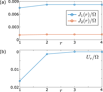
Figure 7: (a) One- and two-site hopping rates $J_{1}(r)$ and $J_{2}(r)$ versus distance $r$ between the two excitations. (b) Interaction potential $U_{r}$ of Eq. (47), for $V^{ee}_{1}=0$. The parameters are $\Delta/\Omega=10$, $D_{1}/\Omega=1$ and $V^{se}_{1}/\Omega=1$.

For $\Delta\gg\Omega,D_{1}\gg D_{2},V^{es}_{1}$, the excitation hopping rates of Eqs. (44) can be well approximated by $r$-independent rates

$$J_{d}\simeq\frac{\Omega^{2}D_{d}}{\Delta^{2}}\propto 1/d^{3}.$$ (45)

Consider next the effective interaction between the excitations. The total energy of $L$ atoms in a lattice with two $\ket{e}$ excitations is

$$E_{2}(x,y)=\sum_{z\neq x,y}\delta^{(x,y)}_{z}.$$ (46)

This sum has now $L-2$ terms and it depends on the positions $x$ and $y$ of the two excitations as per Eq. (39). Due to translational invariance of the lattice, $E_{2}(r)$ depends only on the relative distance $r=|x-y|$. For large $r$, $E_{2}(r)$ tends to a constant since each dressed ground state atom can have at most one excited atom in its vicinity. Setting $E_{2}(r\to\infty)$ as the zero point energy, we can then define the interaction potential between the two excitations as

$$U_{r}=E_{2}(r)-E_{2}(r\to\infty).$$ (47)

Setting, as before, $V^{se}_{d\geq 2}=0$ and $D_{d\geq 3}=0$, we obtain an effective interaction potential $U_{r}$ having range $d_{U}=3$,

$$U_{1}= V^{ee}_{1}-2\left(\frac{\Omega^{2}}{\Delta}-\frac{\Omega^{2}}{\Delta+V^{se}_{1}}\right)$$

$$+2\frac{\Omega^{2}D_{1}^{2}}{(\Delta+V^{se}_{1})^{2}}\left(\frac{2}{\Delta+V^{ie}_{1}}-\frac{1}{\Delta+2V^{se}_{1}}\right)$$

$$+2\Omega^{2}D_{2}^{2}\left(\frac{2}{\Delta^{3}}-\frac{1}{\Delta^{2}(\Delta+V^{se}_{1})}-\frac{1}{(\Delta+V^{se}_{1})^{3}}\right),$$ (48a)

$$U_{2}= V^{ee}_{2}-\left(\frac{\Omega^{2}}{\Delta}-\frac{\Omega^{2}}{\Delta+V^{se}_{1}}\right)$$

$$+2\frac{\Omega^{2}D_{1}^{2}}{\Delta+V^{se}_{1}}\left(\frac{1}{(\Delta+V^{se}_{1})^{2}}-\frac{1}{(\Delta+2V^{se}_{1})^{2}}\right)$$

$$+2\frac{\Omega^{2}D_{2}^{2}}{\Delta^{3}},$$ (48b)

$$U_{3} =V^{ee}_{3}+2\frac{\Omega^{2}D_{2}^{2}}{\Delta}\left(\frac{1}{\Delta^{2}}-\frac{1}{(\Delta+V^{se}_{1})^{2}}\right),$$ (48c)

where for consistency we included the interactions $V^{ee}_{r}$ up to range $d_{U}=3$. In Fig. 7(b) we show the interaction potential $U_{r}$ of Eq. (47), i.e., Eqs. (48) without $V^{ee}_{r}$. Clearly, the nearest-neighbor interaction $U_{1}$ is stronger than $U_{r\geq 2}$, neglecting which would correspond to the spin-lattice model studied in the text. We can now write the interaction term of the Hamiltonian as

$$\mathcal{H}^{(2)}_{U}=\sum_{K}\ket{K}\bra{K}\otimes\sum_{r=1}^{3}U_{r}\ket{r}\bra{r},$$ (49)

which has the same form as Eq. (12).

To summarize, the total Hamiltonian for two $\ket{e}$ excitations in a lattice of Rydberg dressed atoms is

$$\mathcal{H}^{(2)}=\mathcal{H}_{J}^{(2)}+\mathcal{H}_{U}^{(2)},$$ (50)

where $\mathcal{H}_{J}^{(2)}$ and $\mathcal{H}_{U}^{(2)}$ are given by Eqs. (I.2.3) and (49), respectively. In Fig. 1(a) of the main text we show the spectrum of this Hamiltonian. The scattering states are insensitive to the variations of $J_{d}(r)$ and $U_{r}$ at short range $r\leq 3$, so the scattering spectrum is well reproduced by the spin-lattice model Hamiltonian with $r$-independent hopping rates $J_{d}$ and only the nearest-neighbor interaction $U_{1}$. The spin-lattice model approximates well also the bound states of Hamiltonian (50), especially for $U_{r}$ dominated by the nearest-neighbor interatomic interaction $V^{ee}_{1}$ and constant $J_{1}$ achieved for $V^{se}_{1}=-D_{2}$, which is used in Fig. 1(a).

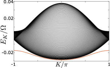
Figure 8: Scattering and bound spectrum for two $\ket{e}$ excitations in a lattice, with the parameters as in Fig. 7.

Note that even without interatomic interactions, $V^{ee}_{r},V^{se}_{r}=0$, we still have non-vanishing effective interaction $U_{1}\simeq 2\frac{\Omega^{2}D_{1}^{2}}{\Delta^{3}}$, which is, however, too weak compared to $J_{1}\simeq\frac{\Omega^{2}D_{1}}{\Delta^{2}}$ to sustain a bound state, see the lower panel of Fig. 3 in the main text. But strong enough interatomic interaction $|V^{se}_{1}|\simeq\Omega,D_{1}\ll\Delta$ resulting in $U_{1}\simeq-2\frac{\Omega^{2}V^{se}_{1}}{\Delta^{2}}$ can sustain two-excitation bound state, as shown in Fig. 8. The corresponding hopping rate $J_{1}(r)$ has now sizable $r$-dependence, see Fig. 7.

Experimental considerations.

A suitable system to realize the spin lattice model and observe the bound states of Rydberg (spin) excitations is a defect-free chain of cold atoms in a one-dimensional optical lattice potential or an array of microtraps Barredo et al. (2016); Endres et al. (2016). The microtraps can be spaced by $a=5-20\>\mu$m, and each microtrap confines the ground state atom within $\Delta a\simeq 1\>\mu$m. We take the atomic parameters similar to those in the recent experiments Béguin et al. (2013); Barredo et al. (2015); Browaeys et al. (2016). The ground state of Rb atoms $\ket{g}=5S_{1/2}$ can be dressed with the Rydberg state $\ket{s}=63P_{1/2}$ by a detuned UV laser with the Rabi frequency $\Omega/(2\pi)\simeq 5\>$MHz and detuning $\Delta/(2\pi)\simeq 33\>$MHz ($\Omega/\Delta=0.15$). The excited Rydberg state $\ket{e}=62D_{3/2}$ can be populated by a two photon transition from the ground state using laser beams focused onto the desired atoms. With the above Rydberg states $\ket{e}$ and $\ket{s}$, the dipole-dipole coefficient for the exchange interaction $D=C_{3}/r^{3}$ is $C_{3}=7950\>$MHz$\>\mu$m³ and the van der Waals coefficient for the interaction $V^{ee}=C_{6}/r^{6}$ is $C_{6}=730\>$GHz$\>\mu$m⁶ Béguin et al. (2013); Barredo et al. (2015); Browaeys et al. (2016). The lifetime of state $\ket{e}$ is $\tau_{e}\simeq 100\>\mu$s, and the dressing state $\ket{s}$ has a similar lifetime $\tau_{s}\simeq 135\>\mu$s but its decay is suppressed by the factor of $\Omega^{2}/\Delta^{2}$.

With the lattice constant $a\simeq 10\>\mu$m, we have $U_{1}\simeq 730\>$kHz $J_{1}\simeq 180\>$kHz and $J_{2}\simeq 22\>$kHz. The hopping rates are larger than the Rydberg state decay rates, which permits observation of coherent dynamics of the Rydberg excitations in the lattice. At the same time, the interaction $U_{1}=4J_{1}$ will support strongly bound states of Rydberg excitations.

The dressed ground state atoms are tightly confined by the microtraps, but the atoms in the Rydberg state are usually not trapped. During the interaction, the Rydberg excited atoms experience a repulsive (or attractive, if $C_{6}<0$) force $F=-\partial_{r}V^{ee}(r)=-6C_{6}/r^{7}$ which can result in their displacement $\Delta r$ from the equilibrium lattice positions. We can estimate the displacement for a pair of atoms at the neighboring lattice sites, $r=a$, as $\Delta r\simeq\frac{F(a)}{2m}t^{2}$, where $m$ is the atomic mass and $t\simeq J_{1,2}^{-1}$ is the timescale of the interaction. We then obtain $\Delta r=3-200\>$nm, which is still smaller than the trap waist $\Delta a$.

We finally note that similar parameters of the spin lattice model can be obtained for atoms in optical lattices with a smaller period $a\lesssim 1\>\mu$m by choosing lower-lying Rydberg states $\ket{s}$ and $\ket{e}$. Such states, however, have shorter lifetimes, which necessitates larger hopping rates $J_{d}$ obtained with stronger dressing lasers. Furthermore, at small interatomic separation, the van der Waals interactions between the untrapped Rydberg-excited atoms will exert stronger force, leading to the displacement of atoms comparable to the lattice spacing. This can be mitigated by using “magic wavelength” optical lattices which simultaneously trap the atoms both in the ground state and the Rydberg state Zhang et al. (2011).