Chemical Abundances of Planetary Nebulae in the Substructures of M31 – II.
The Extended Sample and A Comparison Study with the Outer-disk Group

Abstract

We report deep spectroscopy of ten planetary nebulae (PNe) in the Andromeda Galaxy (M31) using the 10.4 m GTC. Our targets reside in different regions of M31, including halo streams and dwarf satellite M32, and kinematically deviate from the extended disk. The temperature-sensitive [O iii] $\lambda$4363 line is observed in all PNe. For four PNe, the GTC spectra extend beyond 1 $\mu$m, enabling explicit detection of the [S iii] $\lambda$6312 and $\lambda\lambda$9069,9531 lines and thus determination of the [S iii] temperature. Abundance ratios are derived and generally consistent with AGB model predictions. Our PNe probably all evolved from low-mass ($<$2 $M_{\sun}$) stars, as analyzed with the most up-to-date post-AGB evolutionary models, and their main-sequence ages are mostly $\sim$2–5 Gyr. Compared to the underlying, smooth, metal-poor halo of M31, our targets are uniformly metal-rich ([O/H]$\gtrsim-$0.4), and seem to resemble the younger population in the stream. We thus speculate that our halo PNe formed in the Giant Stream’s progenitor through extended star formation. Alternatively, they might have formed from the same metal-rich gas as did the outer-disk PNe, but was displaced into their present locations as a result of galactic interactions. These interpretations are, although speculative, qualitatively in line with the current picture, as inferred from previous wide-field photometric surveys, that M31’s halo is the result of complex interactions and merger processes. The behavior of N/O of the combined sample of the outer-disk and our halo/substructure PNe signifies that hot bottom burning might actually occur at $<$3 $M_{\sun}$, but careful assessment is needed.

1. Introduction

In the cold dark matter ($\Lambda$CDM)-dominated universe, large galaxies formed hierarchically (e.g., White, 1978; White & Rees, 1978) through accretion/merger of smaller subsystems. Such interactions tidally disrupt smaller galaxies and result in extended stellar halo surrounding the central galaxy (e.g., Ibata et al., 2007, 2014). The relics of galaxy interaction and assemblage are registered into the extended halo in forms of stellar streams which, if detected, can be used to study the properties of galaxies and backtrack past interactions (e.g., Ibata et al., 2001a, b, c; Ferguson et al., 2002; Majewski et al., 2003; McConnachie et al., 2009).

Table 1Observing Log and Properties of PNe

PN ID a	R.A.	Decl.	$m_{\lambda 5007}\,^{\rm b}$	$v_{\rm helio}\,^{\rm c}$	$\xi$	$\eta$	$R_{\rm gal}\,^{\rm d}$	Location e	GTC Obs.
	(J2000.0)	(J2000.0)		(km s-1)	($\arcdeg$)	($\arcdeg$)	(kpc)		Grism	Expos.
PN8 (M2430)	00:47:25.9	$+$42:58:59.7	21.32	$-$135.1	0.858	1.720	26.3	Northern Spur	R1000B	2$\times$2400 s
PN9 (M2449)	00:46:13.8	$+$42:40:28.5	20.88	$-$70.6	0.642	1.408	21.2	Northern Spur	R1000B	4$\times$1200 s
									R1000R	2$\times$1200 s
PN10 (LAMOST)	00:44:03.1	$+$42:27:46.6	20.74	$-$234.0	0.242	1.194	16.7	Northern Spur	R1000B	4$\times$1200 s
PN11 (M2432)	00:47:30.3	$+$43:03:40.9	20.69	$-$411.0	0.871	1.798	27.4	Giant Stream	R1000B	4$\times$1200 s
									R1000R	2$\times$1200 s
PN12 (M2466)	00:49:08.0	$+$42:28:44.3	21.96	$-$392.3	1.179	1.220	23.3	Giant Stream	R1000B	4$\times$2400 s
PN13 (LAMOST)	00:49:55.2	$+$38:32:49.0	21.91	$-$362.0	1.404	$-$2.707	41.8	SE Halo	R1000B	4$\times$2400 s
									R1000R	2$\times$1890 s
PN14 (M2507)f	00:48:27.2	$+$39:55:34.3	21.23	$-$146.9	1.095	$-$1.334	23.7	Giant Stream	R1000B	4$\times$2400 s
PN15 (M2512)	00:45:58.5	$+$39:13:25.4	21.10	$-$318.2	0.627	$-$2.042	29.3	SE Halo	R1000B	8$\times$1200 s
PN16 (M2895)	00:42:42.2	$+$40:51:39.8	20.78	$-$193.3	$-$0.007	$-$0.408	5.59	M32	R1000B	6$\times$1200 s
PN17 (LAMOST)	00:53:38.6	$+$41:09:32.1	21.15	$-$437.0	2.052	$-$0.078	28.1	Eastern Halo g	R1000B	5$\times$2100 s
									R1000R	2$\times$1800 s
PN18 (M2234)	00:42:42.3	$+$40:51:49.5	20.13	$-$147.3	$-$0.006	$-$0.405	5.56	M32	R1000B	6$\times$1000 s
NOTE. – PN18 was discarded from analysis because no nebular emission lines were detected in its spectrum.

^a

Number in the bracket is the ID from Merrett et al. (2006) except PN10, PN13 and PN17, which were discovered and identified in the LAMOST survey (Yuan et al., 2010).

^b

From Merrett et al. (2006), except PN10, PN13 and PN17, whose $m_{\lambda 5007}$ are adopted from Yuan et al. (2010).

^c

From Merrett et al. (2006), except PN10, PN13 and PN17, whose $v_{\rm helio}$ are adopted from Yuan et al. (2010).

^d

Sky-projected galactocentric distance estimated at a distance of 785 kpc to M31 (McConnachie et al., 2005).

^e

Here “Halo” means that the PN belongs to the outer halo, or is associated with some substructure.

^f

PN nature confirmed by the LAMOST survey (Yuan et al., 2010).

^g

Might be associated with the NE Shelf, as explained in Section 4.4.

The Andromeda Galaxy (M31) is a nearby (785 kpc, McConnachie et al., 2005) large spiral system and an ideal candidate for studying galaxy formation and evolution. Wide-field surveys, such as PAndAS, have revealed in M31’s outer halo a wealth of large-scale stellar substructures extending to nearly 150 kpc from the galactic centre (e.g., Ibata et al., 2001a, 2007; Ferguson et al., 2002; McConnachie et al., 2003, 2004, 2009; Irwin et al., 2005; Tanaka et al., 2010), with the Northern Spur and the southern Giant Stellar Stream (hereafter the Giant Stream, Ibata et al. 2001a; Caldwell et al. 2010) among the first discovered. The Giant Stream threads to the southeast halo, as far as $>$4$\arcdeg$ from the centre of M31 (Ibata et al., 2001a; McConnachie et al., 2003). The Northern Spur is a feature with enhanced density in metal-rich red giant branch (RGB) stars, located at $\sim$2$\arcdeg$ towards the north (Ferguson et al., 2002).

Planetary nebulae (PNe) are descendants of low- and intermediate-mass ($\sim$1–8 $M_{\sun}$) stars, which account for the majority of stellar populations in our universe. Given their bright, narrow emission lines, PNe are excellent tracers of the chemistry, dynamics and stellar populations of their host galaxies. In the optical spectrum of a PN, the bright [O iii] $\lambda$5007 nebular line alone can carry $\sim$10% of the central star’s energy (e.g., Schönberner et al., 2007). PNe thus are well detected in distant galaxies, even as far as $>$100 Mpc (e.g., Gerhard et al., 2005, 2007; Longobardi et al., 2015a, b). Spectroscopy of PNe in M31, mainly in the bulge and disk (e.g., Jacoby & Ciardullo, 1999; Richer et al., 1999; Kwitter et al., 2012) has found a slightly negative gradient in the oxygen abundance within 50 kpc in the disk (Kwitter et al., 2012). However, recent observations with large (8–10 m) telescopes found that the outer-disk PNe, as far as 100 kpc from the centre of M31, have nearly solar abundances (Balick et al., 2013; Corradi et al., 2015). Even some of the PNe associated with the substructures have O/H close to the Sun (Fang et al., 2013, 2015). These metal-rich PNe in the outskirts of M31 seem to have different origins from the ancient halo, which formed through galaxy mergers long time ago (e.g., Ibata et al., 2007, 2014).

One long-standing, unresolved question is what the origin of M31’s stellar substructure is. It has been proposed that the Northern Spur and the Giant Stream might be connected by a stellar stream (Ferguson et al., 2002; Merrett et al., 2003), of which the dwarf satellite M32 could be the origin (Ibata et al., 2001a; Merrett et al., 2003), but this hypothesis needs assessment. In pursuit of answering this question, we have carried out deep spectroscopic observations of ten bright PNe associated with the two substructures and mostly located in the outer halo (Fang et al., 2013, 2015, hereafter Papers I and II, respectively), and found that they are in overall metal-rich ([O/H]$\sim-$0.3–0) and their oxygen abundances are consistent within the errors (although some internal scatter exists). These abundance analyses led to a tempting, yet tentative, conclusion that the Giant Stream and the Northern Spur might have the same origin. Given the vast extension and complexity of M31’s halo (Ibata et al., 2007, 2014), our sample of PNe so far observed, although representative, is still too limited for us to draw any definite conclusion.

That both the PNe on the halo streams and those kinematically belonging to the extended disk of M31 have been found to be metal-rich ($\sim$solar) is unexpected for a classical, metal-poor halo, and leads to a question of whether they have the same origin (or even population). A comparison study between our halo sample and the disk objects may shed light on this conundrum. Previous attempts have proved that PNe are a very efficient probe of different regions of M31. It is thus possible not only to assess the connection and origin of different substructures, which has been the motivation of our observations so far, but also to make a census study of the extended halo of M31, using PNe as a tool.

In order to better understand the merging history of M31’s halo, we recently carried out deep spectroscopy of eleven PNe: three in the Northern Spur, three associated with the Giant Stream, two in M32, and another three located in the eastern and southeast halo regions. The immediate objectives of the new observations are 1) to obtain accurate abundances (mainly oxygen) for an extended sample, 2) to make a comparison study with the outer-disk PNe in terms of abundance and stellar population, and 3) to assess whether M32 is related to the Northern Spur and the Giant Stream. Being the third paper targeting the PNe in the substructures of M31, this paper is the second one of a series to report deep spectroscopy with a 10 m class telescope. Section 2 introduces target selection and describes the observations and data reduction. Section 3 present emission line measurements, plasma diagnostics and abundance determinations. We present in-depth discussion in Section 4 based on the results, and give summary and conclusions in Section 5.

2. Observations and Data Reduction

2.1. Target Selection:
The Spatial and Kinematical Distribution

Before introducing target selection, we brief some definitions in terms of boundaries in M31 structurre. We adopted the M31 bulge radius ($\sim$3.4 kpc) from the surface brightness fitting by Irwin et al. (2005). The inner disk of M31 is defined at $R_{25}$ (=95′, de Vaucouleurs et al., 1991), which corresponds to 21.7 kpc at the distance of M31; this radius well encompasses the optical disk of M31. Beyond $R_{25}$ lies the extended disk that stretches to 40 kpc, with detections as far as $\sim$70 kpc (Ibata et al., 2005). In the current paper, all M31 PNe beyond $R_{25}$ but with kinematics consistent with the extended disk are dubbed the outer-disk PNe. Previous spectroscopic observations of Kwitter et al. (2012), Balick et al. (2013) and Corradi et al. (2015) all focused on the outer-disk PNe in M31.

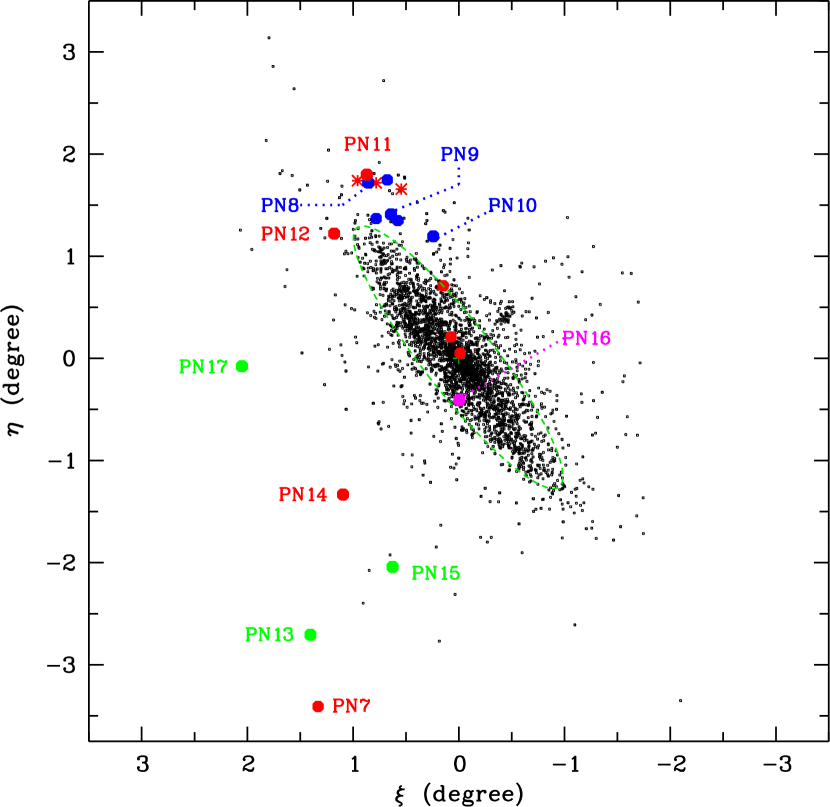
Figure 1.— Spatial distribution of PNe in M31. Objects are from Merrett et al. (2006), Hurley-Keller et al. (2004), Yuan et al. (2010) and Kniazev et al. (2014). Our GTC targets (including those in Paper II) are highlighted with color-filled circles, which are color-coded according to their locations (see Table 1). The three Northern Spur PNe from Paper I are indicated by red asterisks. Coordinates $\xi$ and $\eta$ (given in Table 1) are the M31-based reference frame defined by Huchra et al. (1991). The green dashed ellipse represents the optical disk of M31 with radius $R_{25}$=95′ (de Vaucouleurs et al., 1991), assuming an inclination angle of 77$\fdg$7 (de Vaucouleurs, 1958) and a position angle of 37$\fdg$7 (Merrett et al., 2006) for the M31 disk.

In Papers I and II, we targeted the PNe in the Northern Spur and the Giant Stream substructures. Since our targets kinematically deviate from the extended disk of M31 and are mostly located in the halo, hereafter we call them the halo PNe, to avoid possible confusion with the outer-disk PNe. For the new GTC observations, we selected a sample that covers not only the substructures, but also more extended areas in the M31 system such as the eastern and the southeast halo regions and dwarf satellite M32. The locations/hosts of our targets are given in Table 1, where other properties such as target positions (right ascension–R.A., declination–Decl.), visual magnitudes in [O iii] $\lambda$5007 ($m_{\lambda 5007}$), heliocentric velocities $v_{\rm helio}$ (in km s^-1), angular distances to the centre of M31, and the sky-projected galactocentric distances (in kpc) are also presented. Spatial locations of our targets, including those studied in Papers I and II, are shown in Figure 1. Our halo nebulae are mostly outside $R_{25}$.

We selected eight PNe from the catalog of Merrett et al. (2006) and three from Yuan et al. (2010); the latter was based on a spectroscopic survey at the Large Sky Area Multi-Object Fiber Spectroscopic Telescope (LAMOST, Su et al., 1998; Cui et al., 2004, 2010, 2012; Zhao et al., 2012). These new targets were named PN8–PN18 (see Table 1 and Figure 1), following the target naming (PN1–PN7) in Paper II. According to their locations in M31, our GTC samples PN1–PN17 are highlighted with different colors in Figure 1, where PN16 and PN18 are too close to each other and visually indistinguishable. The [O iii] brightnesses of the new sample are $m_{\lambda 5007}$ $\sim$20.48–21.96, extending down to nearly 1.8 mag from the bright-end cut-off of the planetary nebula luminosity function (PNLF) of M31 (Merrett et al., 2006; Ciardullo et al., 1989; Ciardullo, 2010).

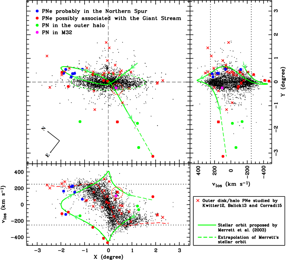
Figure 2.— Spatial and kinematical distribution of PNe in M31 (description of the $X$ and $Y$ coordinates is given the text). Source of the PN samples are the same as in Figure 1. The three Northern Spur PNe studied in Paper I indicated by red asterisks. The seven PNe studied in Paper II and the ten PNe in this work are highlighted (see the legend). The red crosses “$\times$” are the outer-disk PNe studied by Kwitter et al. (2012, Kwitter12), Balick et al. (2013, Balick13), and Corradi et al. (2015, Corradi15). In the upper-left panel: over-plotted is the stellar orbit proposed by Merrett et al. (2003, thick green curve; reproduced with kind permission of the authors). In the two side panels (bottom and right): a projection of the orbit in line-of-sight velocity with respect to M31, $v_{\rm los}$, versus distance along the major and minor axes of M31 is superimposed on the PNe data. Velocities of PNe have been corrected for the systemic velocity $-$306 km s^-1 of M31 (Corbelli et al., 2010). The red dashed curve in the bottom panel is the H i rotation curve from Carignan et al. (2006).

Yuan et al. (2010) did not assign their newly discovered PNe to any locations (i.e., substructure or the extended disk). We identified the locations of the three LAMOST targets (PN10, PN13 and PN17) according to their kinematics shown in Figure 2, which also presents the distribution of the line-of-sight velocity with respect to the centre of M31, $v_{\rm los}$, versus distance along the major and minor axes of M31. The kinematics of PN10 obviously deviates from the extended disk of M31 and is somewhat close to the Northern Spur sample identified by Merrett et al. (2006, Figure 32 therein). We thus identified PN10 as a possible Northern Spur object. PN13 visually resides on the southeast (SE) extension of the Giant Stream; PN15 also seems to be on the stream. However, the velocities of these two PNe, although both deviating from the kinematics of the extended disk, are inconsistent with the stellar orbit of Merrett et al. (2003). PN17 is located in the eastern halo, 2$\fdg$05 from the centre of M31. Its velocity differs significantly from the disk, and its location seems to be very close to the NE Shelf (Ferguson et al., 2005). We temporarily assign PN13, PN15 and PN17 to be the halo nebulae; detailed discussion is in Section 4. The PN nature of PN14 (ID 2507 in Merrett et al. 2006) was confirmed in the LAMOST survey; it might be associated with the Giant Stream. For the other targets selected from Merrett et al. (2006), we adopted their locations identified by the authors (Table 1).

2.2. Spectroscopic Observations

Deep spectroscopy of M31 PNe were carried out with the Optical System for Imaging and low-intermediate-Resolution Integrated Spectroscopy (OSIRIS) spectrograph on the 10.4 m Gran Telescopio Canarias (GTC) at Observatorio de El Roque de los Muchachos (ORM, La Palma). These observations were obtained from 2016 September 2 to 2016 September 11 for GTC program No. GTC25-16B (PI: X. Fang) in service mode. The OSIRIS grism R1000B (1000 lines mm^-1), which covers $\sim$3630–7850 Å, and a long slit with 1$\farcs$0 width were used. The OSIRIS detector is a combination of two 2048$\times$4096 CCDs. The pixel size is 15 $\mu$m, corresponding to 0$\farcs$127 in angular size. We adopted the standard observing mode where the output images were binned by 2$\times$2. The above instrument setup produces a spectral resolution of $\sim$5.5 Å (full width at half-maximum, FWHM) in the blue part of the spectrum and 6.4 Å in the red, at a dispersion of $\sim$2.072 Å pixel^-1. The ideal observing conditions at the ORM provided photometric and clear nights, and excellent seeing (0$\farcs$6–0$\farcs$8) for most of the observations. Moon was also close to dark during the observations. Throughout the observations, the long slit was placed along the parallactic angles to minimize light loss due to atmospheric diffraction. The typical physical sizes of PNe are $\lesssim$0.5 pc (e.g., Frew et al., 2016), corresponding to $\lesssim$0$\farcs$13 in angular size at the distance of M31. This is smaller than the binned CCD pixel size (0$\farcs$254) of OSIRIS, and thus our targets are all point sources and supposed to be well accommodated within the GTC 1″-wide long slit.

In order to remove cosmic rays and to avoid saturation of strong emission lines, multiple exposures were made for each target PN. These exposures are summarized in Table 1. In total, 30 hours observations were completed at the GTC for eleven targets. Thanks to the large light-collecting area of the GTC, we could clearly see almost all the PNe in the direct acquisition CCD image with an exposure of a few seconds (e.g., Figure 3), and then placed the GTC long slit on the targets. Blind offset was utilized only for the two PNe in M32 due to their close proximity ($\sim$7$\farcs$4 and 15$\farcs$4) to the centre of M32. Exposures of spectrophotometric standard stars Ross 640 and G191-B2B (Oke, 1974, 1990) were made in each night to calibrate fluxes for the target spectra, using a slit width of 2$\farcs$52. The HgAr and neon arc line images were obtained (with both 1$\farcs$0 and 2$\farcs$52 slit widths) for wavelength calibration and geometric rectification. Other basic calibration files, such as bias and spectral flats, were also obtained for both the target PN and the standard spectrophotometric star on each night.

We also obtained long-slit spectroscopy of four PNe (PN9, PN11, PN13 and PN17) using the GTC OSIRIS red grism R1000R that covers $\sim$5080–10370 Å. These observations were obtained on 2016 August 23–24 for program No. GTC66-16A (PI: X. Fang). Slit width was 1$\farcs$0, and spectral resolution FWHM$\sim$6.7 Å in the blue region and 8.5 Å in the red, with a dispersion of 2.59 Å pixel^-1. The R1000R exposures are summarized in Table 1. The HgAr, neon and xenon arc lines were used for wavelength calibration. Spectrophotometric standard stars for flux calibration were the same as in the R1000B spectroscopy. Data were obtained under photometric conditions, with seeing $\sim$0$\farcs$8–1$\farcs$0.

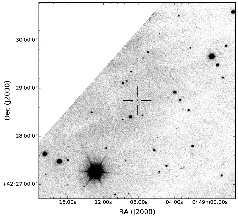
Figure 3.— Negative grey-scale GTC OSIRIS $g$-band acquisition image of PN12 (marked with the black crosshair) taken with an exposure of 5 s.

2.3. Data Reduction

The GTC OSIRIS long-slit spectra were reduced using iraf v2.16. Data reduction generally followed the standard procedure, similar to what has been described in Fang et al. (2015). The raw PN spectral images were first bias-subtracted and corrected for flat-field. We then performed wavelength calibration using HgAr arc lines for the PN spectra obtained with the R1000B grism, and HgAr+Xe for the R1000R spectra. Although geometry distortion along the long slit does not affect the nebular emission lines of our targets, which are point sources on CCD, such distortion of the sky lines must be corrected for so that background subtraction can be properly done. During the wavelength calibration, we rectified geometry distortion by fitting the arc lines using third-order polynomial functions in the two-dimensional (2D) spectrogram. This geometry rectification “straightened” the sky lines along the slit.

We subtracted the background from each single exposure of the target frame by fitting the background emission along the slit direction using high-order cubic spline functions (see more details in Fang et al. 2015). We then combined the background-subtracted 2D frames of the same PN to remove the cosmic rays. We then used the FILTER/COSMIC task in the software midas v13SEPpl1.2 to further eliminate any possible cosmic residuals in the CCD images. The above procedures produced a well “cleaned” spectral image for each PN, which was then flux-calibrated (and also corrected for the atmospheric extinction) using the spectrum of spectrophotometric standards.

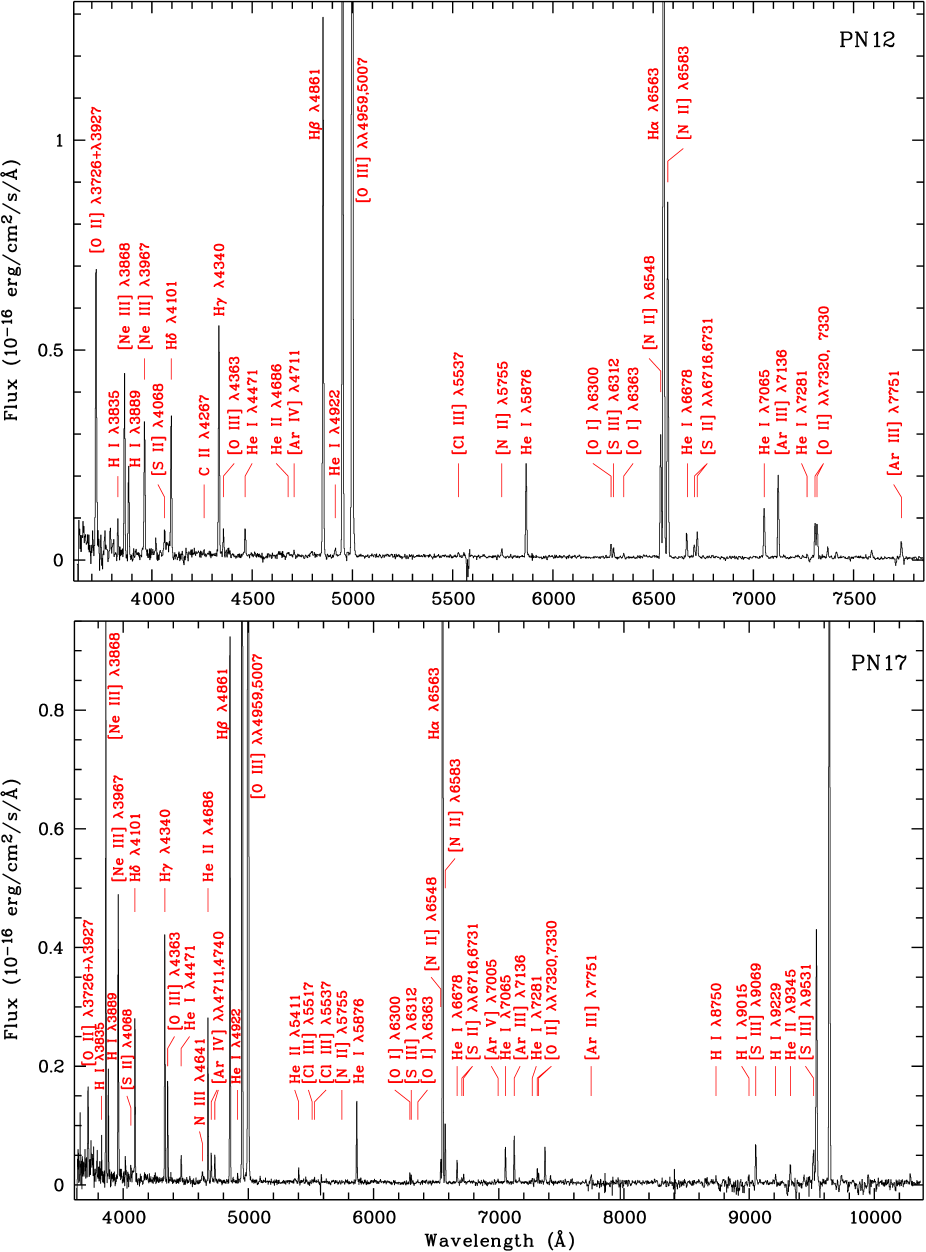
Figure 4.— GTC OSIRIS spectrum of PN12 (top) and PN17 (bottom). The spectrum of PN12 was obtained using the R1000B grism, while the spectrum of PN17 is a combination of the R1000B ($\leq$7500 Å) and R1000R ($>$7500 Å) spectra. Vertical ranges of both panels are set to accommodate the intensity of H$\beta$. All important emission lines are labeled. Extinction has not been corrected for. For PN12, the weak features between [O ii] $\lambda\lambda$7320,7330 and [Ar iii] $\lambda$7751 are the second-order effect. In the spectrum of PN17, the strong emission features redward of [S iii] $\lambda$9531 are also due to the second-order contamination.

Table 2Fluxes and Intensities

Ion	$\lambda$	Transition	PN8		PN9		PN10		PN11		PN12
	(Å)		$F$($\lambda$)	$I$($\lambda$)	$F$($\lambda$)	$I$($\lambda$)	$F$($\lambda$)	$I$($\lambda$)	$F$($\lambda$)	$I$($\lambda$)	$F$($\lambda$)	$I$($\lambda$)
$[$O ii$]$	3727a	2p3 4So–2p3 2Do	19.6	22.4$\pm$2.5	50.3	57.3$\pm$5.2	29.3	35.1$\pm$3.9	32.9	39.4$\pm$4.3	59.7	68.2$\pm$5.5
H i	3798	2p 2Po–10d 2D	$\cdots$	$\cdots$	3.72	4.22$\pm$0.94	3.34	3.96$\pm$0.90	3.15	3.74$\pm$0.83	4.55	5.17$\pm$1.05
H i	3835	2p 2Po–9d 2D	3.12	3.53$\pm$1.00	5.74	6.48$\pm$1.83	4.78	5.65$\pm$1.60	6.24	7.38$\pm$2.01	4.93	5.58$\pm$1.17
$[$Ne iii$]$	3868	2p4 3P2–2p4 1D2	107	120$\pm$8	82.4	92.8$\pm$6.2	76.5	90.0$\pm$6.0	100	117$\pm$8	29.2	33.0$\pm$2.2
H i	3889b	2p 2Po–8d 2D	5.75	6.48$\pm$0.97	15.5	17.4$\pm$2.6	12.4	14.6$\pm$2.20	15.1	17.8$\pm$2.6	14.4	16.2$\pm$2.4
$[$Ne iii$]$	3967c	2p4 3P1–2p4 1D2	46.2	51.6$\pm$4.0	38.5	43.0$\pm$3.3	36.0	41.8$\pm$3.2	50.0	58.2$\pm$4.5	27.7	31.0$\pm$2.3
He i	4026	2p 3Po–5d 3D	1.48	1.64$\pm$0.85	2.53	2.79$\pm$1.45	1.50	1.73$\pm$0.89	0.46	0.53$\pm$:	2.21	2.45$\pm$1.27
$[$S ii$]$	4068d	3p3 4S${}^{\rm o}_{3/2}$–3p3 2P${}^{\rm o}_{3/2}$	9.05	10.0$\pm$1.5	2.73	3.01$\pm$0.45	1.91	2.18$\pm$0.33	4.88	5.58$\pm$0.83	5.32	5.88$\pm$0.87
H i	4101	2p 2Po–6d 2D	27.0	29.8$\pm$3.1	23.0	25.2$\pm$2.6	22.8	25.9$\pm$2.7	29.4	33.5$\pm$3.4	27.5	30.3$\pm$3.1
C ii	4267	3d 2D–4f 2Fo	$\cdots$	$\cdots$	$\cdots$	$\cdots$	$\cdots$	$\cdots$	1.38	1.52$\pm$0.27	0.79	0.85$\pm$0.31
H i	4340e	2p 2Po–5d 2D	42.5	45.3$\pm$3.3	43.5	46.4$\pm$3.5	42.0	45.7$\pm$3.3	40.1	43.7$\pm$3.1	42.2	45.0$\pm$3.2
$[$O iii$]$	4363	2p2 1D2–2p2 1S0	9.43	10.0$\pm$1.2	8.20	8.71$\pm$1.04	8.19	8.90$\pm$1.07	12.4	13.5$\pm$1.6	4.20	4.47$\pm$0.53
He i	4388	2p 1P${}^{\rm o}_{1}$–5d 1D2	$\cdots$	$\cdots$	$\cdots$	$\cdots$	$\cdots$	$\cdots$	$\cdots$	$\cdots$	1.13	1.20$\pm$0.54
He i	4471	2p 3Po–4d 3D	5.61	5.88$\pm$0.82	4.38	4.59$\pm$0.74	4.47	4.76$\pm$0.66	4.88	5.21$\pm$0.84	5.47	5.74$\pm$0.82
N iii	4641f	3p 2P${}^{\rm o}_{3/2}$–3d 2D5/2	$\cdots$	$\cdots$	$\cdots$	$\cdots$	$\cdots$	$\cdots$	3.44	3.57$\pm$0.72	$\cdots$	$\cdots$
C iii	4649g	3s 3S–3p 3Po	$\cdots$	$\cdots$	1.46	1.50$\pm$0.67	$\cdots$	$\cdots$	$\cdots$	$\cdots$	$\cdots$	$\cdots$
He ii	4686	3d 2D–4f 2Fo	1.21	1.23$\pm$0.40	1.52	1.55$\pm$0.50	$\cdots$	$\cdots$	13.0	13.2$\pm$1.1	0.87	0.89$\pm$0.18
$[$Ar iv$]$	4711h	3p3 4S${}^{\rm o}_{3/2}$–3p3 2D${}^{\rm o}_{5/2}$	1.72	1.75$\pm$0.53	1.14	1.16$\pm$0.35	1.34	1.37$\pm$0.41	4.28	4.38$\pm$0.66	0.81	0.83$\pm$0.20
$[$Ar iv$]$	4740	3p3 4S${}^{\rm o}_{3/2}$–3p3 2D${}^{\rm o}_{3/2}$	2.87	2.91$\pm$0.55	1.38	1.40$\pm$0.26	1.18	1.20$\pm$0.35	4.32	4.40$\pm$0.82	$\cdots$	$\cdots$
H i	4861e	2p 2Po–4d 2D	100	100	100	100	100	100	100	100	100	100
He i	4922	2p 1P${}^{\rm o}_{1}$–4d 1D2	0.74	0.73$\pm$:	0.72	0.71$\pm$:	1.16	1.15$\pm$0.63	1.03	1.02$\pm$0.61	1.49	1.48$\pm$0.67
$[$O iii$]$	4959	2p2 1P1–2p2 1D2	438	433$\pm$17	425	420$\pm$16	354	349$\pm$13	474.1	467$\pm$18	189	187$\pm$7
$[$O iii$]$	5007	2p2 1P2–2p2 1D2	1307	1286$\pm$25	1286	1266$\pm$24	1068	1046$\pm$20	1450	1420$\pm$26	569	560$\pm$11
$[$N i$]$	5198i	2p3 4S${}^{\rm o}_{3/2}$–2p3 2D${}^{\rm o}_{3/2}$	0.77	0.74$\pm$:	$\cdots$	$\cdots$	0.56	0.53$\pm$:	$\cdots$	$\cdots$	$\cdots$	$\cdots$
He ii	5411	4f 2Fo–7g 2G	$\cdots$	$\cdots$	$\cdots$	$\cdots$	$\cdots$	$\cdots$	1.47	1.37$\pm$0.36	$\cdots$	$\cdots$
$[$Cl iii$]$	5537	3p3 4S${}^{\rm o}_{3/2}$–3p3 2D${}^{\rm o}_{3/2}$	1.71	1.60$\pm$0.47	$\cdots$	$\cdots$	$\cdots$	$\cdots$	0.55	0.51$\pm$0.28	0.58	0.54$\pm$0.31
$[$N ii$]$	5755	2p2 1D2–2p2 1S0	2.42	2.24$\pm$0.49	1.46	1.36$\pm$0.30	1.10	1.00$\pm$0.22	1.04	0.94$\pm$0.20	1.47	1.36$\pm$0.26
C iv	5805	3s 2S–3p 2Po	$\cdots$	$\cdots$	9.29	8.59$\pm$0.95	$\cdots$	$\cdots$	$\cdots$	$\cdots$	$\cdots$	$\cdots$
He i	5876	2p 3Po–3d 3D	17.5	16.1$\pm$1.8	18.5	17.1$\pm$1.8	15.6	14.0$\pm$1.2	16.4	14.6$\pm$1.3	17.2	15.8$\pm$1.7
$[$O i$]$	6300	2p4 3P2–2p4 1D2	4.22	3.78$\pm$1.24	7.19	6.46$\pm$2.12	5.12	4.42$\pm$1.45	2.38	2.05$\pm$0.67	2.38	2.13$\pm$0.50
$[$S iii$]$	6312j	3p2 1D2–3p2 1S0	2.87	2.57$\pm$0.64	1.25	1.13$\pm$0.41	1.31	1.13$\pm$0.41	1.75	1.50$\pm$0.54	1.45	1.30$\pm$0.47
$[$O i$]$	6363	2p4 3P1–2p4 1D2	1.60	1.43$\pm$1.20	1.52	1.36$\pm$1.14	1.64	1.41$\pm$1.18	0.62	0.53$\pm$0.44	0.51	0.46$\pm$0.40
$[$N ii$]$	6548	2p2 3P1–2p2 1D2	15.8	14.0$\pm$1.5	19.8	17.5$\pm$2.0	10.2	8.65$\pm$0.92	13.0	11.0$\pm$1.2	23.6	20.9$\pm$2.4
H i	6563e	2p 2Po–3d 2D	304	284$\pm$13	322	285$\pm$15	287	283$\pm$12	293	283$\pm$13	301	284$\pm$14
$[$N ii$]$	6583	2p2 3P2–2p2 1D2	53.7	47.4$\pm$4.2	62.0	55.0$\pm$4.9	29.8	25.2$\pm$2.2	39.8	33.6$\pm$2.9	73.0	64.4$\pm$5.7
He i	6678k	2p 1P${}^{\rm o}_{1}$–3d 1D2	5.26	4.62$\pm$0.65	4.73	4.17$\pm$0.58	4.00	3.36$\pm$0.47	4.35	3.65$\pm$0.50	4.64	4.07$\pm$0.56
$[$S ii$]$	6716	3p3 4S${}^{\rm o}_{3/2}$–3p3 2D${}^{\rm o}_{5/2}$	1.87	1.64$\pm$0.34	2.42	2.13$\pm$0.44	1.03	0.86$\pm$0.20	2.23	1.86$\pm$0.38	2.38	2.10$\pm$0.43
$[$S ii$]$	6731	3p3 4S${}^{\rm o}_{3/2}$–3p3 2D${}^{\rm o}_{3/2}$	2.31	2.02$\pm$0.38	4.23	3.71$\pm$0.50	1.68	1.41$\pm$0.26	4.24	3.54$\pm$0.42	4.98	4.36$\pm$0.44
He i	7065	2p 3Po–3s 3S	9.96	8.55$\pm$1.03	11.5	9.93$\pm$1.20	10.7	8.76$\pm$1.05	8.25	6.72$\pm$0.81	10.7	9.23$\pm$1.11
$[$Ar iii$]$	7136	3p4 3P2–3p4 1D2	19.3	16.5$\pm$1.6	14.8	12.7$\pm$1.23	12.3	10.0$\pm$1.10	18.0	14.5$\pm$1.4	17.1	14.7$\pm$1.4
He i	7281	2p 1P${}^{\rm o}_{1}$–3s 1S0	$\cdots$	$\cdots$	0.43	0.36$\pm$:	$\cdots$	$\cdots$	0.44	0.36$\pm$:	0.34	0.29$\pm$:
$[$O ii$]$	7320	2p3 2D${}^{\rm o}_{5/2}$–2p3 2P${}^{\rm o}_{3/2}$	10.1	8.59$\pm$1.11	6.88	5.84$\pm$0.75	7.91	6.33$\pm$0.82	2.36	1.88$\pm$0.24	6.55	5.55$\pm$0.71
$[$O ii$]$	7330	2p3 2D${}^{\rm o}_{3/2}$–2p3 2P${}^{\rm o}_{3/2}$	8.54	7.23$\pm$1.10	5.78	4.91$\pm$0.74	6.19	4.95$\pm$0.75	1.83	1.46$\pm$0.22	7.20	6.10$\pm$0.91
$[$Ar iii$]$	7751	3p4 3P1–3p4 1D2	3.05	2.52$\pm$0.63	2.24	1.86$\pm$0.46	2.24	1.74$\pm$0.78	3.89	3.00$\pm$0.74	2.96	2.45$\pm$0.60
H i	8750	3d 2D–12f 2Fo	$\cdots$	$\cdots$	1.72	1.36$\pm$0.41	$\cdots$	$\cdots$	1.57	1.14$\pm$0.34	$\cdots$	$\cdots$
H i	9015	3d 2D–10f 2Fo	$\cdots$	$\cdots$	1.85	1.45$\pm$0.43	$\cdots$	$\cdots$	1.31	0.94$\pm$0.27	$\cdots$	$\cdots$
$[$S iii$]$	9069	3p2 3P1–3p2 1D2	$\cdots$	$\cdots$	21.5	17.0$\pm$1.4	$\cdots$	$\cdots$	22.7	16.2$\pm$1.3	$\cdots$	$\cdots$
H i	9229	3d 2D–9f 2Fo	$\cdots$	$\cdots$	2.26	1.76$\pm$0.62	$\cdots$	$\cdots$	7.52	5.34$\pm$1.88	$\cdots$	$\cdots$
He ii	9345	5g 2G–8h 2Ho	$\cdots$	$\cdots$	5.14	4.00$\pm$1.3	$\cdots$	$\cdots$	3.55	2.51$\pm$0.81	$\cdots$	$\cdots$
$[$S iii$]$	9531l	3p2 3P1–3p2 1D2	$\cdots$	$\cdots$	17.4	13.5$\pm$1.6	$\cdots$	$\cdots$	14.4	10.1$\pm$1.2	$\cdots$	$\cdots$
$c$(H$\beta$)			0.181		0.177		0.243		0.245		0.180
$\log$ $F$(H$\beta$)m			$-$15.29		$-$15.09		$-$14.92		$-$15.04		$-$15.09
Ion	$\lambda$	Transition	PN13		PN14		PN15		PN16		PN17
	(Å)		$F$($\lambda$)	$I$($\lambda$)	$F$($\lambda$)	$I$($\lambda$)	$F$($\lambda$)	$I$($\lambda$)	$F$($\lambda$)	$I$($\lambda$)	$F$($\lambda$)	$I$($\lambda$)
$[$O ii$]$	3727a	2p3 4So–2p3 2Do	44.1	50.1$\pm$5.8	24.2	27.5$\pm$3.0	63.2	74.4$\pm$8.2	71.5	76.3$\pm$9.2	23.5	27.1$\pm$2.4
H i	3798	2p 2Po–10d 2D	$\cdots$	$\cdots$	5.68	6.44$\pm$1.43	$\cdots$	$\cdots$	13.0	13.8$\pm$2.8	4.21	4.83$\pm$1.01
H i	3835	2p 2Po–9d 2D	3.72	4.19$\pm$1.10	3.82	4.32$\pm$1.00	3.07	3.57$\pm$0.91	$\cdots$	$\cdots$	5.63	6.44$\pm$1.14
$[$Ne iii$]$	3868	2p4 3P2–2p4 1D2	43.0	48.1$\pm$3.1	40.2	45.2$\pm$2.8	80.5	93.2$\pm$4.7	122	130$\pm$10.4	93.0	106$\pm$8
H i	3889b	2p 2Po–8d 2D	12.6	14.1$\pm$2.0	13.3	15.0$\pm$2.1	12.3	14.2$\pm$1.9	3.87	4.10$\pm$2.1	16.4	18.6$\pm$2.6
$[$Ne iii$]$	3967c	2p4 3P1–2p4 1D2	28.2	31.3$\pm$2.4	27.3	30.4$\pm$2.5	41.3	47.2$\pm$2.8	60.2	63.5$\pm$6.4	51.2	57.7$\pm$4.7
He i	4026	2p 3Po–5d 3D	1.73	1.91$\pm$0.78	1.89	2.09$\pm$0.85	1.03	1.17$\pm$0.67	$\cdots$	$\cdots$	3.18	3.56$\pm$0.64
$[$S ii$]$	4068d	3p3 4S${}^{\rm o}_{3/2}$–3p3 2P${}^{\rm o}_{3/2}$	2.56	2.81$\pm$0.62	5.57	6.14$\pm$0.91	4.10	4.61$\pm$0.86	8.41	8.82$\pm$1.06	2.40	2.67$\pm$0.53

Table 2(Continued)

H i

4101

2p 2Po–6d 2D

22.8

25.0$\pm$2.4

24.9

27.4$\pm$2.8

24.4

27.4$\pm$2.0

25.2

26.4$\pm$3.7

28.0

31.1$\pm$2.2

C iii

4187

4f 1F${}^{\rm o}_{3}$–5g 1G4

$\cdots$

$\cdots$

$\cdots$

$\cdots$

$\cdots$

$\cdots$

$\cdots$

$\cdots$

1.03

1.13$\pm$0.24

He ii

4199

4f 2Fo–11g 2G

$\cdots$

$\cdots$

$\cdots$

$\cdots$

$\cdots$

$\cdots$

$\cdots$

$\cdots$

1.05

1.15$\pm$0.27

H i

4340e

2p 2Po–5d 2D

42.0

44.5$\pm$3.2

40.8

43.5$\pm$3.0

39.3

42.5$\pm$3.1

60.2

62.1$\pm$6.5

41.2

44.2$\pm$3.2

$[$O iii$]$

4363

2p2 1D2–2p2 1S0

4.02

4.26$\pm$0.51

5.62

5.97$\pm$0.67

5.31

5.73$\pm$0.68

11.0

11.4$\pm$1.3

15.6

16.7$\pm$1.7

He i

4388

2p 1P${}^{\rm o}_{1}$–5d 1D2

$\cdots$

$\cdots$

$\cdots$

$\cdots$

$\cdots$

$\cdots$

$\cdots$

$\cdots$

1.27

1.36$\pm$0.31

He i

4471

2p 3Po–4d 3D

5.23

5.47$\pm$0.88

4.31

4.52$\pm$0.70

4.45

4.72$\pm$0.76

4.91

5.02$\pm$0.71

4.03

4.24$\pm$0.68

N iii

4641f

3p 2P${}^{\rm o}_{3/2}$–3d 2D5/2

$\cdots$

$\cdots$

$\cdots$

$\cdots$

$\cdots$

$\cdots$

$\cdots$

$\cdots$

2.63

2.71$\pm$0.52

C iv

4658

5g 2G–6h 2Ho

$\cdots$

$\cdots$

$\cdots$

$\cdots$

1.52

1.57$\pm$0.22

$\cdots$

$\cdots$

$\cdots$

$\cdots$

He ii

4686

3d 2D–4f 2Fo

$\cdots$

$\cdots$

$\cdots$

$\cdots$

2.03

2.08$\pm$0.24

21.5

21.7$\pm$2.3

26.0

26.6$\pm$2.4

$[$Ar iv$]$

4711h

3p3 4S${}^{\rm o}_{3/2}$–3p3 2D${}^{\rm o}_{5/2}$

0.94

0.96$\pm$0.17

$\cdots$

$\cdots$

1.06

1.10$\pm$0.17

$\cdots$

$\cdots$

4.95

5.05$\pm$0.90

$[$Ar iv$]$

4740

3p3 4S${}^{\rm o}_{3/2}$–3p3 2D${}^{\rm o}_{3/2}$

$\cdots$

$\cdots$

$\cdots$

$\cdots$

1.40

1.43$\pm$0.20

$\cdots$

$\cdots$

4.76

4.83$\pm$0.91

H i

4861e

2p 2Po–4d 2D

100

100

100

100

100

100

100

100

100

100

He i

4922

2p 1P${}^{\rm o}_{1}$–4d 1D2

1.48

1.47$\pm$0.87

0.73

0.73$\pm$0.43

1.96

1.94$\pm$0.64

$\cdots$

$\cdots$

1.01

1.00$\pm$0.40

$[$O iii$]$

4959

2p2 1P1–2p2 1D2

295

292$\pm$11

232

230$\pm$9

427

421$\pm$16

564

561$\pm$28

497

491$\pm$18

$[$O iii$]$

5007

2p2 1P2–2p2 1D2

891

878$\pm$16

710

699$\pm$13

1275

1250$\pm$23

1693

1680$\pm$31

1519

1493$\pm$27

$[$N i$]$

5198i

2p3 4S${}^{\rm o}_{3/2}$–2p3 2D${}^{\rm o}_{3/2}$

$\cdots$

$\cdots$

0.65

0.63$\pm$:

$\cdots$

$\cdots$

$\cdots$

$\cdots$

$\cdots$

$\cdots$

He ii

5411

4f 2Fo–7g 2G

$\cdots$

$\cdots$

$\cdots$

$\cdots$

$\cdots$

$\cdots$

$\cdots$

$\cdots$

1.95

1.85$\pm$0.33

$[$Cl iii$]$

5517

3p3 4S${}^{\rm o}_{3/2}$–3p3 2D${}^{\rm o}_{5/2}$

$\cdots$

$\cdots$

$\cdots$

$\cdots$

$\cdots$

$\cdots$

$\cdots$

$\cdots$

0.46

0.43$\pm$:

$[$Cl iii$]$

5537

3p3 4S${}^{\rm o}_{3/2}$–3p3 2D${}^{\rm o}_{3/2}$

$\cdots$

$\cdots$

$\cdots$

$\cdots$

$\cdots$

$\cdots$

$\cdots$

$\cdots$

0.57

0.53$\pm$0.26

$[$N ii$]$

5755

2p2 1D2–2p2 1S0

0.43

0.40$\pm$:

1.12

1.04$\pm$0.22

1.26

1.15$\pm$0.21

$\cdots$

$\cdots$

0.34

0.31$\pm$:

C iv

5805

3s 2S–3p 2Po

$\cdots$

$\cdots$

$\cdots$

$\cdots$

16.1

14.6$\pm$1.6

$\cdots$

$\cdots$

$\cdots$

$\cdots$

He i

5876

2p 3Po–3d 3D

15.0

13.8$\pm$1.2

16.1

14.8$\pm$1.4

17.0

15.3$\pm$1.3

15.5

15.0$\pm$1.4

14.8

13.5$\pm$1.2

$[$O i$]$

6300

2p4 3P2–2p4 1D2

3.42

3.08$\pm$0.61

1.49

1.34$\pm$0.30

3.75

3.28$\pm$0.65

$\cdots$

$\cdots$

1.54

1.37$\pm$0.27

$[$S iii$]$

6312j

3p2 1D2–3p2 1S0

1.97

1.78$\pm$0.38

1.38

1.24$\pm$0.34

2.53

2.22$\pm$0.52

$\cdots$

$\cdots$

0.92

0.82$\pm$0.26

$[$O i$]$

6363

2p4 3P1–2p4 1D2

1.27

1.14$\pm$0.54

0.39

0.35$\pm$0.18

1.25

1.09$\pm$0.53

$\cdots$

$\cdots$

0.48

0.43$\pm$:

$[$N ii$]$

6548

2p2 3P1–2p2 1D2

10.8

9.62$\pm$1.05

8.77

7.77$\pm$0.95

22.0

18.9$\pm$2.1

72.3

68.1$\pm$7.4

4.25

3.72$\pm$0.40

H i

6563e

2p 2Po–3d 2D

290

286$\pm$13

256

284$\pm$12

281

287$\pm$12

290

285$\pm$14

299

282$\pm$13

$[$N ii$]$

6583

2p2 3P2–2p2 1D2

30.8

27.3$\pm$2.0

24.6

21.8$\pm$1.8

63.8

54.7$\pm$4.0

255

240$\pm$18

11.4

9.93$\pm$0.72

He i

6678k

2p 1P${}^{\rm o}_{1}$–3d 1D2

4.08

3.60$\pm$0.49

4.26

3.75$\pm$0.58

4.24

3.61$\pm$0.49

$\cdots$

$\cdots$

4.15

3.60$\pm$0.49

$[$S ii$]$

6716

3p3 4S${}^{\rm o}_{3/2}$–3p3 2D${}^{\rm o}_{5/2}$

2.12

1.87$\pm$0.34

1.00

0.87$\pm$0.18

3.23

2.74$\pm$0.50

12.1

11.3$\pm$2.0

0.90

0.78$\pm$0.14

$[$S ii$]$

6731

3p3 4S${}^{\rm o}_{3/2}$–3p3 2D${}^{\rm o}_{3/2}$

4.40

3.87$\pm$0.52

1.45

1.27$\pm$0.19

5.29

4.49$\pm$0.60

16.8

15.8$\pm$2.1

1.53

1.32$\pm$0.17

$[$Ar v$]$

7005

3p2 3P2–3p2 1D2

$\cdots$

$\cdots$

$\cdots$

$\cdots$

$\cdots$

$\cdots$

$\cdots$

$\cdots$

0.44

0.38$\pm$:

He i

7065

2p 3Po–3s 3S

9.04

7.82$\pm$1.17

10.2

8.81$\pm$1.40

8.83

7.34$\pm$1.10

$\cdots$

$\cdots$

6.70

5.68$\pm$0.85

$[$Ar iii$]$

7136

3p4 3P2–3p4 1D2

12.8

11.1$\pm$1.10

9.00

7.72$\pm$0.90

19.8

16.4$\pm$1.7

13.7

12.7$\pm$1.6

8.10

6.84$\pm$0.68

He i

7281

2p 1P${}^{\rm o}_{1}$–3s 1S0

$\cdots$

$\cdots$

$\cdots$

$\cdots$

$\cdots$

$\cdots$

$\cdots$

$\cdots$

0.57

0.47$\pm$:

$[$O ii$]$

7320

2p3 2D${}^{\rm o}_{5/2}$–2p3 2P${}^{\rm o}_{3/2}$

6.76

5.78$\pm$0.74

8.39

7.13$\pm$1.05

3.65

2.98$\pm$0.38

6.84

6.31$\pm$0.82

1.92

1.60$\pm$0.20

$[$O ii$]$

7330

2p3 2D${}^{\rm o}_{3/2}$–2p3 2P${}^{\rm o}_{3/2}$

5.75

4.90$\pm$0.73

8.16

6.94$\pm$1.21

3.58

2.92$\pm$0.44

11.2

10.3$\pm$1.5

1.44

1.20$\pm$0.17

$[$Ar iii$]$

7751

3p4 3P1–3p4 1D2

2.08

1.73$\pm$0.43

1.18

0.98$\pm$0.30

3.63

2.88$\pm$0.72

6.07

5.53$\pm$1.37

1.17

0.96$\pm$0.23

H i

8750

3d 2D–12f 2Fo

1.57

1.25$\pm$0.37

$\cdots$

$\cdots$

$\cdots$

$\cdots$

$\cdots$

$\cdots$

1.63

1.25$\pm$0.37

H i

9015

3d 2D–10f 2Fo

4.54

3.59$\pm$1.03

$\cdots$

$\cdots$

$\cdots$

$\cdots$

$\cdots$

$\cdots$

1.48

1.13$\pm$0.32

$[$S iii$]$

9069

3p2 3P1–3p2 1D2

37.8

30.0$\pm$2.4

$\cdots$

$\cdots$

$\cdots$

$\cdots$

$\cdots$

$\cdots$

13.0

9.86$\pm$0.78

H i

9229

3d 2D–9f 2Fo

2.84

2.23$\pm$0.78

$\cdots$

$\cdots$

$\cdots$

$\cdots$

$\cdots$

$\cdots$

2.15

1.64$\pm$0.57

He ii

9345

5g 2G–8h 2Ho

6.81

5.34$\pm$1.72

$\cdots$

$\cdots$

$\cdots$

$\cdots$

$\cdots$

$\cdots$

4.98

3.77$\pm$1.21

$[$S iii$]$

9531l

3p2 3P1–3p2 1D2

55.4

43.3$\pm$6.1

$\cdots$

$\cdots$

$\cdots$

$\cdots$

$\cdots$

$\cdots$

12.2

9.22$\pm$1.20

$c$(H$\beta$)

0.172

0.177

0.220

0.087

0.196

$\log$ $F$(H$\beta$)m

$-$15.34

$-$15.07

$-$15.45

$-$15.29

$-$15.21

NOTE. – Fluxes and intensities are normalized such that H$\beta$=100. Colon “:” indicates that the uncertainty in line intensity is large ($>$100%).

^a

A blend of the O ii $\lambda$3726 (2p^3 4S${}^{\rm o}_{3/2}$–2p^3 2D${}^{\rm o}_{3/2}$) and $\lambda$3729 (2p^3 4S${}^{\rm o}_{3/2}$–2p^3 2D${}^{\rm o}_{5/2}$) doublet.

^b

Blended with the He i $\lambda$3888 (2s ³S–3p ${3}$P^o) line.

^c

Blended with H i $\lambda$3970 (2p ²P^o–7d ²D) and He i $\lambda$3965 (2s ¹S–4p ¹P^o).

^d

Blended with [S ii] $\lambda$4076; probably also blended with the weak O ii M10 3p ⁴D^o–3d ⁴F and C iii M16 4f ³F^o–5g ³G lines.

^e

Corrected for the flux from the blended He ii line.

^f

Blended with the N iii $\lambda\lambda$4634,4642 lines; probably also blended with O ii M1 $\lambda\lambda$4639,4642.

^g

Blended with the O ii M2 3s ⁴P–3p ⁴D^o lines.

^h

Corrected for the flux from the blended He i $\lambda$4713 (2p ³P^o–4s ³S) line.

ⁱ

Blended with [N i] $\lambda$5200 (2p^3 4S${}^{\rm o}_{3/2}$–2p^3 2D${}^{\rm o}_{5/2}$).

^j

Corrected for the flux from the blended He ii $\lambda$6311 (5g ²G–16h ²H^o) line.

^k

Corrected for the flux from the blended He ii $\lambda$6683 (5g ²G–13h ²H^o) line.

^l

Flux underestimated due to the second-order contamination beyond 9200 Å.

^m

In units of erg cm^-2 s^-1, as measured in the extracted spectrum.

We extracted a 1D spectrum on the fully calibrated 2D frame of each PN for spectral analysis. As an example, Figure 4 shows the 1D spectra for PN12 and PN17 in our sample. In the common wavelength region (5080–7850 Å) covered by the R1000B and R1000R grisms, differences in the fluxes of emission lines (He i $\lambda\lambda$5876,6678,7065, [N ii] $\lambda\lambda$6548,6583, H$\alpha$, [S ii] $\lambda$6716,6731, [Ar iii] $\lambda$7136, [O ii] $\lambda\lambda$7320,7330) detected in both spectra of PN9, PN11, PN13 and PN17 are mostly less than 5%. We corrected for the effect of second-order contamination in the red part of the R1000B spectrum (Figure4, top) following the method of Fang et al. (2015). For the R1000R grism, the second-order contamination exists beyond 9200 Å (Figure 4, bottom). Fortunately, this contamination only affects the [S iii] $\lambda$9531 emission line. The [S iii] $\lambda$9069 nebular line was unaffected.

Despite careful data reduction, detection of emission lines in one (target PN18) of the two PNe in M32 failed due to its close proximity (7$\farcs$4) to the bright nucleus of M32, although this target is the brightest in our sample. The other M32 PN (PN16) is 15$\farcs$4 from M32’s centre and has good data quality. We thus analyzed ten PNe (PN8–PN17; Table 1) in this paper.

3. Results and Analysis

3.1. Emission Line Fluxes

The emission line fluxes were measured from the extracted 1D spectra by integrating over line profiles. The observed line fluxes of all targets, normalized to $F$(H$\beta$)=100, are presented in Table 2, where the observed H$\beta$ fluxes (in erg cm^-2 s^-1) are also presented. The R1000R spectrum was scaled according to the H$\alpha$ line flux in the R1000B spectrum. We derived the logarithmic extinction parameter, $c$(H$\beta$), by comparing the observed and theoretical ratios of hydrogen Balmer lines, H$\alpha$/H$\beta$ and H$\gamma$/H$\beta$. The theoretical Case B H i line ratios were adopted from Storey & Hummer (1995) at an electron temperature of 10 000 K and a density of 10⁴ cm^-3. The $c$(H$\beta$) values of our PNe are small (0.08-0.25) and are presented in Table 2. The observed line fluxes were then dereddened using the formula

$$I(\lambda)=10^{c(\rm{H}\beta)[1+{\it f}(\lambda)]}F(\lambda),$$ (1)

where $f$($\lambda$) is the extinction curve of Cardelli et al. (1989) with a total-to-selective extinction ratio $R_{V}$ = 3.1. The extinction corrected line intensities, all normalized to $I$(H$\beta$) = 100, along with the measurement errors, are presented in Table 2. Given the excellent observing conditions (seeing$<$1$\farcs$0) and the slit width (1$\farcs$0), light loss in strong emission lines is expected to be negligible.

3.2. Plasma Diagnostics

We carried out plasma diagnostics of PNe using the ratios of the extinction-corrected fluxes of the collisionally excited lines (CELs; also often called forbidden lines) of heavy elements in Table 2. The [S ii] $\lambda$6716/$\lambda$6731 ratio is a common density diagnostic. Where available, intensity ratio of the fainter [Ar iv] $\lambda\lambda$4711,4740 lines was also used to derive the electron density; here the flux of the blended He i $\lambda$4713 line was corrected for using the theoretical He i line ratios calculated by Porter et al. (2012). The electron temperature was derived from the [O iii] ($\lambda$4959+$\lambda$5007)/$\lambda$4363 nebular-to-auroral line ratio. The [N ii] temperature was also determined whenever the [N ii] $\lambda$5755 line was detected. References for the atomic data utilized in plasma diagnostics as well as the ionic-abundance determinations (in Section 3.3) are summarized in Table 3, where sources of the effective recombination coefficients for the optical recombination lines (ORLs) analyzed in the paper are also given. Results of plasma diagnostics are presented in Table 4.

Table 3References for Atomic Data

Ion	CELs
	Transition Probabilities	Collision Strengths
N+	Bell et al. (1995)	Stafford et al. (1994)
O+	Zeippen (1987)	Pradhan et al. (2006)
O2+	Storey & Zeippen (2000)	Lennon & Burke (1994)
Ne2+	Landi & Bhatia (2005)	McLaughlin & Bell (2000)
S+	Keenan et al. (1993)	Ramsbottom et al. (1996)
S2+	Mendoza & Zeippen (1982a)	Tayal & Gupta (1999)
Ar2+	Biémont & Hansen (1986)	Galavis et al. (1995)
Ar3+	Mendoza & Zeippen (1982b)	Ramsbottom et al. (1997)
Ar4+	Mendoza & Zeippen (1982a)	Mendoza (1983)
Ion	ORLs
	Effective Recombination Coeff.	Comments
H i	Storey & Hummer (1995)	Case B
He i	Porter et al. (2012)	Case B
He ii	Storey & Hummer (1995)	Case B
C ii	Davey et al. (2000)	Case B

Only in two PNe (PN12 and PN13) did we find that $T_{\rm e}$([N ii]) is reasonably lower than $T_{\rm e}$([O iii]). In the other targets (except PN16), $T_{\rm e}$([N ii])$>T_{\rm e}$([O iii]). This might be due to high-density clumps in PNe (Morisset, 2016): at high densities ($N_{\rm e}\gtrsim$10⁵ cm^-3), emission of the [N ii] $\lambda\lambda$6548,6583 nebular lines can be suppressed due to collisional deexcitation (while emission of the $\lambda$5755 auroral line is unaffected), and consequently the [N ii] temperature is overestimated. Results of plasma diagnostics based on the CELs are visually demonstrated in Figure 5, where the diagnostic curves of different forbidden-line ratios are plotted for each PN. The fortran code equib, which was originally developed by Howarth & Adams (1981) to solve the statistical equilibrium equations of multi-level atoms to derive level populations and line emissivities under given nebular physical conditions, was used for the plasma diagnostics.

Other temperature-sensitive ratios are [O ii] $\lambda$3727/($\lambda$7320+$\lambda$7330) and [S ii] ($\lambda$6716+$\lambda$6731)/$\lambda$4072, where $\lambda$3727 is a blend of the [O ii] $\lambda\lambda$3726,3729 doublet, and $\lambda$4072 is a blend of [S ii] $\lambda\lambda$4068,4076. However, not in all PNe did we detect these faint auroral lines to a desired S/N. For the four PNe for which the OSIRIS R1000R spectroscopy was obtained, we also derived the temperature using the [S iii] ($\lambda$9069+$\lambda$9531)/$\lambda$6312 line ratio. Since the [S iii] $\lambda$9531 nebular line was affected by the second-order contamination (see Section 2.3), we assumed a theoretical ratio $\lambda$9531/$\lambda$9069 = 2.48 (Mendoza & Zeippen, 1982a; Mendoza, 1983) to derive the intrinsic flux of this [S iii] line. Besides the traditional CEL diagnostics, we also determined the electron temperatures using the He i ORLs. These He i temperatures were generally lower than those derived from the CELs (Table 4), consistent with Paper II. The principles of PN plasma diagnostics based on the He i ORLs are described in Zhang et al. (2005).

Table 4Plasma Diagnostics

Diagnostic Ratio	PN8	PN9	PN10	PN11	PN12
	$T_{\mathrm{e}}$ (K)
$[$O iii$]$ ($\lambda$4959+$\lambda$5007)/$\lambda$4363	10 680$\pm$400	10 200$\pm$300	10 960$\pm$370	11 300$\pm$400	10 500$\pm$340
$[$N ii$]$ ($\lambda$6548+$\lambda$6583)/$\lambda$5755	20 000$\pm$5000	12 200$\pm$1300	16 300$\pm$3900	12 200$\pm$2300	9200$\pm$2200
$[$O ii$]$ $\lambda$3727/($\lambda$7320+$\lambda$7330)	$>$20 000	17 200$\pm$6000	$>$20 000	7500$\pm$2500	7300$\pm$2700
$[$S iii$]$ ($\lambda$9069+$\lambda$9531)/$\lambda$6312	$\cdots$	10 700$\pm$1100	$\cdots$	12 700$\pm$1500	$\cdots$
$[$S ii$]$ ($\lambda$6716+$\lambda$6731)/$\lambda$4072 a	$\cdots$	$\cdots$	$\cdots$	$\cdots$	9200$\pm$2800
He i $\lambda$5876/$\lambda$4471	10 000$\pm$4000	$\cdots$	5600$\pm$3000	8000$\pm$3500	9400$\pm$3000
He i $\lambda$6678/$\lambda$4471	9300$\pm$4000	3400$\pm$3000	12 600$\pm$7500	12 900$\pm$8000	12 500$\pm$8000
	$N_{\mathrm{e}}$ (cm-3)
$[$S ii$]$ $\lambda$6716/$\lambda$6731	1400$\pm$1000	5200$\pm$2000	3900$\pm$1200	8700$\pm$3800	21 000$\pm$5000
$[$Ar iv$]$ $\lambda$4711/$\lambda$4740	16 200$\pm$5400	7600$\pm$3800	2500$\pm$:	8000$\pm$2700	$\cdots$
$[$O ii$]$ $\lambda$3727/($\lambda$7320+$\lambda$7330)	$>$20 000	14 000$\pm$8000	$\sim$20 000	4000$\pm$2000	12 000$\pm$8000
	PN13	PN14	PN15	PN16	PN17
	$T_{\mathrm{e}}$ (K)
$[$O iii$]$ ($\lambda$4959+$\lambda$5007)/$\lambda$4363	9100$\pm$300	11 000$\pm$370	9100$\pm$250	10 200$\pm$700	12 100$\pm$450
$[$N ii$]$ ($\lambda$6548+$\lambda$6583)/$\lambda$5755	8000$\pm$2000	19 200$\pm$4400	11 400$\pm$2300	$\cdots$	13 600$\pm$2000
$[$O ii$]$ $\lambda$3727/($\lambda$7320+$\lambda$7330)	8300$\pm$3000	$>$20 000	10 200$\pm$2900	$>$20 000	10 900$\pm$2600
$[$S iii$]$ ($\lambda$9069+$\lambda$9531)/$\lambda$6312	10 020$\pm$930	$\cdots$	$\cdots$	$\cdots$	11 400$\pm$2500
$[$S ii$]$ ($\lambda$6716+$\lambda$6731)/$\lambda$4072 a	6000$\pm$2600	$\cdots$	$\cdots$	$>$20 000	$\cdots$
He i $\lambda$5876/$\lambda$4471	$>$20 000	2700$\pm$:	2800$\pm$:	5100$\pm$2500	3200$\pm$:
He i $\lambda$6678/$\lambda$4471	14 700$\pm$8000	6300$\pm$3000	10 200$\pm$5000	$\cdots$	5200$\pm$2000
	$N_{\mathrm{e}}$ (cm-3)
$[$S ii$]$ $\lambda$6716/$\lambda$6731	19 600$\pm$8000	2600$\pm$1400	3700$\pm$1900	2040$\pm$1000	4700$\pm$1500
$[$Ar iv$]$ $\lambda$4711/$\lambda$4740	$\cdots$	$\cdots$	8800$\pm$3400	$\cdots$	6100$\pm$1800
$[$O ii$]$ $\lambda$3727/($\lambda$7320+$\lambda$7330)	$\sim$20 000	$>$20 000	6300$\pm$3000	$>$20 000	6000$\pm$3000
$[$Cl iii$]$ $\lambda$5517/$\lambda$5537	$\cdots$	$\cdots$	$\cdots$	$\cdots$	5500$\pm$2400
NOTE. – The colon “:” indicates very large uncertainty.

^a

A blend of [S ii] $\lambda\lambda$4068, 4076; also blended with O ii M10 3p ⁴D^o–3d ⁴F and C iii M16 4f ³F^o–5g ³G lines.

Uncertainties in the electron temperatures and densities presented in Table 4 were estimated based on the measurement errors of emission line fluxes through propagation. Weaker lines generally have larger measurement errors, as a result introducing larger uncertainties in temperatures/densities. A typical example is [N ii] $\lambda$5755, whose intensity is 10%–30% that of [O iii] $\lambda$4363 for most targets in our sample. Errors in the [N ii] temperatures are systematically higher that those in the [O iii] temperatures, which are thus best measured.

3.3. Ionic Abundances

Using the relative intensities of emission lines in Table 2 and the electron temperatures and densities in Table 4, we calculated the ionic abundances of our PNe. The equib program was used to calculate the ionic abundances of He, C, N, O, Ne, S, Cl and Ar relative to hydrogen, which are presented in Table 5. The deep GTC spectroscopy enabled detection of several faint diagnostic lines, including the [O iii] $\lambda$4363, [N ii] $\lambda$5755, and [S iii] $\lambda$6312 auroral lines. It is thus possible to consider multiple ionization zones within a nebula, i.e., to assign different temperatures/densities when calculating abundances of ionic species with different ionization stages (i.e., the ionization potentials). This is a more realistic paradigm of nebular analysis, and reduces the uncertainties in resultant abundances that may arise from the temperatures assumed.

The [O iii] temperature was used to derive O²⁺/H⁺, Ne²⁺/H⁺, Ar²⁺/H⁺, Ar³⁺/H⁺ and Cl²⁺/H⁺. We adopted the [N ii] temperature to calculate N⁺/H⁺ and O⁺/H⁺ for PN12 and PN13, where we found the [N ii] temperature is lower than that derived from the [O iii] line ratio. For the other PNe, we considered the recipe of Dufour et al. (2015, also ) for the electron temperature in the low-ionization region: if He ii $\lambda$4686 was detected, we adopted an [N ii] temperature of 10 300 K derived by Kaler (1986); otherwise, we assumed a temperature of 10 000 K.

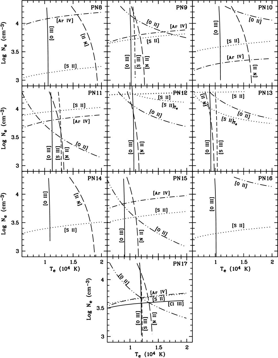
Figure 5.— Plasma diagnostic diagrams. Different line types represent the temperature or density diagnostics using different line ratios (see Table 4 for line ratios). For PN12 and PN13, the dotted line labeled with [S ii]${}_{T_{\rm e}}$ is the temperature-diagnostic curve using the [S ii] ($\lambda$6716+$\lambda$6731)/$\lambda$4072 intensity ratio. The dotted line labeled with [S ii] is density-diagnostic curve for all PNe.

The [S iii] temperature derived for the four PNe (PN9, PN11, PN13 and PN17) is in general meaningfully different from the [O iii] temperature, and thus were used to calculate the S²⁺/H⁺ ratio. For the other PNe, we adopted the electron temperature that was used to calculate the N⁺/H⁺ ratio to derive S²⁺/H⁺. In the calculations of S⁺/H⁺, we adopted the [S ii] temperature (9200 K) for PN12; for the other targets, we adopted the temperature that was used to calculate the N⁺/H⁺ ratio. Although temperatures (or the lower limits) were also derived from the [O ii] $\lambda$3727/($\lambda$7320+$\lambda$7330) line ratio, they were much too different from the [S iii] temperatures (Table 4), given that the ionization potential of O⁺ (35.12 eV) is close to that of S²⁺ (34.83 eV); the differences between the [O ii] temperatures and those derived from the [O iii] lines are also questionable. The only exception is PN17, whose [O ii] temperature seems reasonable compared to those derived from the [O iii] and [S iii] line ratios. We adopted the electron density derived from the [S ii] $\lambda$6716/$\lambda$6731 ratio for the ionic-abundance calculations of the low-ionization species. Where available, the density yielded by [Ar iv] $\lambda$4711/$\lambda$4740 was assumed for the high-ionization species, otherwise the [S ii] density was used. For PN17, the density derived from [Cl iii] $\lambda$5517/$\lambda$5537 was used to derive Cl²⁺/H⁺.

Care must be taken when deriving the O⁺/H⁺ ratio, although O⁺ is not the dominant ionization stage of oxygen in PNe. We noticed that the [O ii] $\lambda$3727 (a blend of $\lambda\lambda$3726,3729) nebular line yielded a very different O⁺/H⁺ ratio from that derived from the [O ii] $\lambda\lambda$7320,7330 auroral lines, if the same electron density was assumed. Such difference in O⁺/H⁺ even reached one order of magnitude for some PNe in our sample. This might be because $\lambda$3727 and $\lambda\lambda$7320,7330 actually come from regions with very different densities. Besides its dependence on temperature, the [O ii] $\lambda$3727/($\lambda$7320+$\lambda$7330) line ratio also has non-negligible dependence on the density, as can be seen in Figure 5. If these two [O ii] lines come from different nebular regions, the diagnosed temperature can be unrealistically high.

If we adopt the [S ii] density for [O ii] $\lambda$3727 and assumed a higher density (e.g., 20 000 cm^-3; Table 4) for $\lambda$7325 (=$\lambda$7320+$\lambda$7330), the two O⁺/H⁺ ratios derived can be brought to the same level (Table 5). Thus the electron densities (or the lower limit, see Table 4) yielded by the [O ii] diagnostic ratio was assumed for the $\lambda$7325 line. We then derived a weighted average from the two O⁺/H⁺ ratios, with the weights proportional to the intensities of the $\lambda$3727 and $\lambda$7325 lines. The averaged O⁺/H⁺ ratio was adopted and then used for the determination of elemental abundances.

Ne²⁺/H⁺ derived from [Ne iii] $\lambda$3868 was adopted; the other [Ne iii] nebular line $\lambda$3967 is blended with H i $\lambda$3970. For the four PNe (PN9, PN11, PN13 and PN17) where both $\lambda$6312 and $\lambda$9069 of [S iii] were detected, a line intensity-weighted average of the S²⁺/H⁺ ratios derived from the two [S iii] lines was adopted. For the other PNe in our sample, S²⁺/H⁺ derived from $\lambda$6312 was adopted. The total intensity of the [Ar iv] $\lambda\lambda$4711,4740 doublet was used to derive Ar³⁺/H⁺. The flux of [Ar iv] $\lambda$4711 was corrected for the blended He i $\lambda$4713 line. The effective recombination coefficients of the He i lines calculated by Porter et al. (2012) was used to derive the He⁺/H⁺ ratios. The He²⁺/H⁺ ratio was derived from He ii $\lambda$4686 using the hydrogenic effective recombination coefficients from Storey & Hummer (1995). We also detected C ii $\lambda$4267 (M6 3d ²D–4f ²F^o) in the spectra of PN11 and PN12, and the C²⁺/H⁺ ratio was derived using this line (Table 5). The Case B effective recombination coefficients of the C ii lines were adopted from Davey et al. (2000), and an electron temperature of 10 000 K and a density of 10⁴ cm^-3 were assumed.

The uncertainties in ionic abundances (in the brackets in Table 5), were estimated from the measurement errors in line fluxes. Extra errors in abundances could be introduced by the electron temperatures and densities adopted in abundance determinations, although we have considered multiple ionization zones by deriving the abundances of low- and high-ionization species using different temperatures/densities. However, these errors in general have minor contribution to the total uncertainty budget, and were not included in the final uncertainties of the ionic abundances. In Paper II we have estimated that errors in the [O iii] temperature typically introduce $\sim$10% uncertainties in the resultant ionic abundances, while in this work such errors are probably even lower. It is evident that the ORLs of heavy elements (C ii, O ii, N ii and Ne ii) observed in PNe could be emitted by nebular regions as cold as $\lesssim$1000 K (e.g., Liu, 2012; Fang & Liu, 2013; McNabb et al., 2013). For an ORL (like C ii $\lambda$4267) excited by radiative recombination, its emissivity (i.e., effective recombination coefficient) generally decreases with the electron temperature (e.g., Osterbrock & Ferland, 2006; Fang & Liu, 2013). Thus C²⁺/H⁺ derived here could be overestimated due to the temperature (10 000 K) assumed. According to the calculations of Davey et al. (2000), the effective recombination coefficient of the C ii $\lambda$4267 line decreases by a factor of 9.4 as the temperature increases from 1000 K to 10 000 K.

3.4. Elemental Abundances

The total elemental abundances (relative to hydrogen) were derived based on the ionic abundances presented in Table 5. The helium abundance is a sum of the ionic ratios, He/H = He⁺/H⁺ + He²⁺/H⁺. For heavy elements, the total abundances were derived mostly using the ionization correction factors (ICFs) of Kingsburgh & Barlow (1994). Elemental abundances are presented in Table 6, and the ICFs used to correct for the unseen ions are presented in Table 7.

In the cases where both S⁺/H⁺ and S²⁺/H⁺ were derived, S/H = ICF(S)$\times$(S⁺/H⁺ + S²⁺/H⁺) was used, where ICF(S) was adopted from Kingsburgh & Barlow (1994, Equation A36 therein). For PN16 where only S⁺/H⁺ was obtainable, the empirical fitting formula of Kingsburgh & Barlow (1994, Equation A38 therein) was used to derive S²⁺/H⁺. If both Ar²⁺ and Ar³⁺ were observed, we used Ar/H = ICF(Ar)$\times$(Ar²⁺/H⁺ + Ar³⁺/H⁺), where ICF(Ar) is from Kingsburgh & Barlow (1994, Equation A30 therein). In typical physical conditions of PNe, concentration of argon in Ar⁴⁺ is supposed to be negligible compared to Ar²⁺ and Ar³⁺. If only Ar²⁺ was observed (in PN12, PN13, PN14 and PN16 in our sample), Equation A32 in Kingsburgh & Barlow (1994) was used to derive ICF(Ar). Only Cl²⁺ was observed in our spectra (of PN8, PN11, PN12 and PN17), and we assumed Cl/Cl²⁺ $\approx$S/S²⁺ as in Wang & Liu (2007), according to similarity in ionization potentials. C/H was derived for two PNe in our sample assuming ICF(C) = O/O²⁺ (Table 6). Delgado-Inglada et al. (2014) developed a new set of formulae for the ICFs of PNe by computing a large grid of photoionization models. These ICFs have validity application ranges defined by the ionic fractions of helium, He²⁺/(He⁺ + He²⁺), and oxygen, O²⁺/(O⁺ + O²⁺). We expect that these ICFs are adequate estimates of elemental abundances in PNe. However, not all our targets have the helium or oxygen ionic fractions located within these validity ranges. Besides, the new ICFs do not differ much from the classical methods of Kingsburgh & Barlow (1994) for most of the elements (García-Rojas et al., 2016). In particular, adopting the new ICFs of Delgado-Inglada et al. (2014) did not eliminate the “sulfur anomaly” in PNe, which is discussed in Section 4.1.

Table 5Ionic Abundances

Ion	Line	Abundance (Xi+/H+)
	(Å)	PN8	PN9	PN10	PN11	PN12
He+	4471	0.105$\pm$0.016	0.087$\pm$0.014	0.090$\pm$0.013	0.099$\pm$0.016	0.109$\pm$0.015
	5876	0.104$\pm$0.012	0.111$\pm$0.012	0.090$\pm$0.010	0.095$\pm$0.008	0.102$\pm$0.011
	6678	0.113$\pm$0.016	0.102$\pm$0.014	0.082$\pm$0.011	0.089$\pm$0.012	0.100$\pm$0.014
Adopteda		0.104$\pm$0.012	0.111$\pm$0.012	0.090$\pm$0.010	0.095$\pm$0.008	0.102$\pm$0.011
He2+	5411	$\cdots$	$\cdots$	$\cdots$	1.47($\pm$0.40)$\times$10-2	$\cdots$
	4686	1.02($\pm$0.28)$\times$10-3	1.28($\pm$0.41)$\times$10-3	$\cdots$	1.10($\pm$0.10)$\times$10-2	0.74($\pm$0.15)$\times$10-3
C2+	4267	$\cdots$	$\cdots$	$\cdots$	1.47($\pm$0.26)$\times$10-3	8.17($\pm$2.98)$\times$10-4
N+	5755	2.26($\pm$0.50)$\times$10-5	1.53($\pm$0.34)$\times$10-5	8.30($\pm$1.83)$\times$10-6	6.09($\pm$1.30)$\times$10-6	1.02($\pm$0.20)$\times$10-5
	6548	6.89($\pm$0.74)$\times$10-6	1.01($\pm$0.12)$\times$10-5	4.12($\pm$0.44)$\times$10-6	5.05($\pm$0.54)$\times$10-6	1.32($\pm$0.15)$\times$10-5
	6583	7.95($\pm$0.70)$\times$10-6	1.08($\pm$0.10)$\times$10-5	4.08($\pm$0.36)$\times$10-6	5.29($\pm$0.46)$\times$10-6	1.39($\pm$0.12)$\times$10-5
Adoptedb		7.95($\pm$0.70)$\times$10-6	1.08($\pm$0.10)$\times$10-5	4.08($\pm$0.36)$\times$10-6	5.29($\pm$0.46)$\times$10-6	1.39($\pm$0.12)$\times$10-5
O+	3727	2.15($\pm$0.24)$\times$10-5	3.58($\pm$0.32)$\times$10-5	1.47($\pm$0.16)$\times$10-5	1.46($\pm$0.18)$\times$10-5	5.82($\pm$0.47)$\times$10-5
	7320	5.54($\pm$0.77)$\times$10-5	5.01($\pm$0.64)$\times$10-5	3.40($\pm$0.44)$\times$10-5	1.30($\pm$0.20)$\times$10-5	4.23($\pm$0.54)$\times$10-5
	7330	5.69($\pm$0.86)$\times$10-5	5.14($\pm$0.75)$\times$10-5	3.24($\pm$0.49)$\times$10-5	1.24($\pm$0.20)$\times$10-5	5.67($\pm$0.64)$\times$10-5
	7325	5.61($\pm$0.86)$\times$10-5	5.07($\pm$0.75)$\times$10-5	3.33($\pm$0.49)$\times$10-5	1.27($\pm$0.20)$\times$10-5	4.88($\pm$0.64)$\times$10-5
Adoptedc		3.58($\pm$0.42)$\times$10-5	3.82($\pm$0.45)$\times$10-5	1.92($\pm$0.25)$\times$10-5	1.45($\pm$0.20)$\times$10-5	5.68($\pm$0.68)$\times$10-5
O2+	4363	3.60($\pm$0.43)$\times$10-4	4.09($\pm$0.50)$\times$10-4	2.68($\pm$0.32)$\times$10-4	3.30($\pm$0.39)$\times$10-4	1.69($\pm$0.20)$\times$10-4
	4959	3.53($\pm$0.14)$\times$10-4	3.96($\pm$0.15)$\times$10-4	2.61($\pm$0.10)$\times$10-4	3.17($\pm$0.12)$\times$10-4	1.65($\pm$0.06)$\times$10-4
	5007	3.63($\pm$0.10)$\times$10-4	4.13($\pm$0.10)$\times$10-4	2.71($\pm$0.06)$\times$10-4	3.34($\pm$0.06)$\times$10-4	1.71($\pm$0.05)$\times$10-4
Adoptedd		3.63($\pm$0.10)$\times$10-4	4.13($\pm$0.10)$\times$10-4	2.71($\pm$0.06)$\times$10-4	3.34($\pm$0.06)$\times$10-4	1.71($\pm$0.05)$\times$10-4
Ne2+	3868	9.40($\pm$0.63)$\times$10-5	8.60($\pm$0.57)$\times$10-5	6.37($\pm$0.43)$\times$10-5	7.34($\pm$0.50)$\times$10-5	2.74($\pm$0.20)$\times$10-5
	3967	9.25($\pm$0.72)$\times$10-5	8.29($\pm$0.64)$\times$10-5	6.07($\pm$0.46)$\times$10-5	8.76($\pm$0.68)$\times$10-5	4.12($\pm$0.31)$\times$10-5
Adoptede		9.40($\pm$0.63)$\times$10-5	8.60($\pm$0.57)$\times$10-5	6.37($\pm$0.43)$\times$10-5	7.34($\pm$0.50)$\times$10-5	2.74($\pm$0.20)$\times$10-5
S+	6716	9.00($\pm$1.86)$\times$10-8	2.43($\pm$0.50)$\times$10-7	7.10($\pm$1.65)$\times$10-8	2.32($\pm$0.47)$\times$10-7	1.39($\pm$0.28)$\times$10-7
	6731	8.99($\pm$1.69)$\times$10-8	2.43($\pm$0.32)$\times$10-7	7.10($\pm$1.11)$\times$10-8	2.33($\pm$0.28)$\times$10-7	2.10($\pm$0.21)$\times$10-7
Adopted		8.99($\pm$1.69)$\times$10-8	2.43($\pm$0.32)$\times$10-7	7.10($\pm$1.12)$\times$10-8	2.33($\pm$0.30)$\times$10-7	2.10($\pm$0.22)$\times$10-7
S2+	6312	4.69($\pm$1.17)$\times$10-6	2.39($\pm$0.44)$\times$10-6	1.82($\pm$0.50)$\times$10-6	2.03($\pm$0.46)$\times$10-6	2.38($\pm$0.38)$\times$10-6
	9069	$\cdots$	3.65($\pm$0.30)$\times$10-6	$\cdots$	2.59($\pm$0.21)$\times$10-6	$\cdots$
	9531	$\cdots$	5.28($\pm$0.78)$\times$10-7	$\cdots$	2.94($\pm$0.41)$\times$10-7	$\cdots$
Adoptedf		4.69($\pm$1.17)$\times$10-6	3.57($\pm$0.31)$\times$10-6	1.82($\pm$0.50)$\times$10-6	2.54($\pm$0.22)$\times$10-6	2.38($\pm$0.38)$\times$10-6
Cl2+	5537	1.83($\pm$0.46)$\times$10-7	$\cdots$	$\cdots$	4.57($\pm$1.80)$\times$10-8	6.69($\pm$2.72)$\times$10-8
Ar2+	7136	1.30($\pm$0.12)$\times$10-6	1.11($\pm$0.13)$\times$10-6	7.46($\pm$0.77)$\times$10-7	1.01($\pm$0.13)$\times$10-6	1.20($\pm$0.11)$\times$10-6
	7751	8.32($\pm$2.07)$\times$10-7	6.79($\pm$2.01)$\times$10-7	5.40($\pm$1.35)$\times$10-7	8.70($\pm$2.16)$\times$10-7	8.35($\pm$2.00)$\times$10-7
Adoptedg		1.30($\pm$0.12)$\times$10-6	1.11($\pm$0.13)$\times$10-6	7.46($\pm$0.77)$\times$10-7	1.01($\pm$0.13)$\times$10-6	1.20($\pm$0.11)$\times$10-6
Ar3+	4711	2.35($\pm$0.58)$\times$10-7	2.10($\pm$0.63)$\times$10-7	1.81($\pm$0.41)$\times$10-7	5.52($\pm$0.83)$\times$10-7	$\cdots$
	4740	4.90($\pm$0.60)$\times$10-7	2.39($\pm$0.44)$\times$10-7	1.81($\pm$0.38)$\times$10-7	5.36($\pm$0.88)$\times$10-7	$\cdots$
Adopted		4.90($\pm$0.60)$\times$10-7	2.39($\pm$0.44)$\times$10-7	1.81($\pm$0.38)$\times$10-7	5.36($\pm$0.88)$\times$10-7	$\cdots$
	(Å)	PN13	PN14	PN15	PN16	PN17
He+	4471	0.104$\pm$0.015	0.086$\pm$0.013	0.090$\pm$0.013	0.095$\pm$0.013	0.081$\pm$0.012
	5876	0.089$\pm$0.008	0.096$\pm$0.010	0.099$\pm$0.008	0.096$\pm$0.012	0.088$\pm$0.008
	6678	0.088$\pm$0.013	0.092$\pm$0.014	0.089$\pm$0.013	$\cdots$	0.088$\pm$0.011
Adopteda		0.089$\pm$0.008	0.096$\pm$0.010	0.099$\pm$0.008	0.096$\pm$0.012	0.088$\pm$0.008
He2+	5411	$\cdots$	$\cdots$	$\cdots$	$\cdots$	2.00($\pm$0.36)$\times$10-2
	4686	$\cdots$	$\cdots$	1.73($\pm$0.20)$\times$10-3	1.80($\pm$0.22)$\times$10-2	2.21($\pm$0.20)$\times$10-2
N+	5755	6.21($\pm$:)$\times$10-6	8.82($\pm$1.87)$\times$10-6	2.47($\pm$0.45)$\times$10-5	$\cdots$	1.65($\pm$:)$\times$10-6
	6548	8.91($\pm$0.97)$\times$10-6	3.61($\pm$0.44)$\times$10-6	1.48($\pm$0.16)$\times$10-5	3.81($\pm$0.41)$\times$10-5	1.42($\pm$0.15)$\times$10-6
	6583	8.61($\pm$0.63)$\times$10-6	3.43($\pm$0.28)$\times$10-6	1.45($\pm$0.11)$\times$10-5	4.57($\pm$0.40)$\times$10-5	1.29($\pm$0.10)$\times$10-6
Adoptedb		8.61($\pm$0.63)$\times$10-6	3.43($\pm$0.28)$\times$10-6	1.45($\pm$0.11)$\times$10-5	4.57($\pm$0.40)$\times$10-5	1.29($\pm$0.10)$\times$10-6
O+	3727	1.13($\pm$0.13)$\times$10-4	9.96($\pm$1.10)$\times$10-6	4.08($\pm$0.45)$\times$10-5	3.57($\pm$0.48)$\times$10-5	1.25($\pm$0.11)$\times$10-5
	7320	9.55($\pm$1.22)$\times$10-5	3.74($\pm$0.55)$\times$10-5	2.94($\pm$0.37)$\times$10-5	5.10($\pm$0.66)$\times$10-5	1.20($\pm$0.15)$\times$10-5
	7330	9.89($\pm$1.27)$\times$10-5	4.43($\pm$0.61)$\times$10-5	3.52($\pm$0.43)$\times$10-5	1.02($\pm$0.15)$\times$10-4	1.10($\pm$0.16)$\times$10-5
	7325	9.70($\pm$1.25)$\times$10-5	4.05($\pm$0.60)$\times$10-5	3.20($\pm$0.43)$\times$10-5	7.39($\pm$1.05)$\times$10-5	1.16($\pm$0.17)$\times$10-5
Adoptedc		1.10($\pm$0.14)$\times$10-4	2.03($\pm$0.33)$\times$10-5	4.01($\pm$0.45)$\times$10-5	4.25($\pm$0.76)$\times$10-5	1.24($\pm$0.12)$\times$10-5
O2+	4363	4.31($\pm$0.52)$\times$10-4	1.76($\pm$0.20)$\times$10-4	6.07($\pm$0.72)$\times$10-4	5.47($\pm$0.86)$\times$10-4	2.84($\pm$0.30)$\times$10-4
	4959	4.23($\pm$0.16)$\times$10-4	1.70($\pm$0.07)$\times$10-4	6.00($\pm$0.23)$\times$10-4	5.32($\pm$0.30)$\times$10-4	2.73($\pm$0.10)$\times$10-4
	5007	4.40($\pm$0.08)$\times$10-4	1.79($\pm$0.04)$\times$10-4	6.15($\pm$0.11)$\times$10-4	5.52($\pm$0.13)$\times$10-4	2.88($\pm$0.05)$\times$10-4
Adoptedd		4.40($\pm$0.10)$\times$10-4	1.79($\pm$0.05)$\times$10-4	6.15($\pm$0.12)$\times$10-4	5.52($\pm$0.15)$\times$10-4	2.88($\pm$0.05)$\times$10-4
Ne2+	3868	7.25($\pm$0.47)$\times$10-5	3.15($\pm$0.20)$\times$10-5	1.41($\pm$0.10)$\times$10-4	1.22($\pm$0.13)$\times$10-4	5.29($\pm$0.40)$\times$10-5
	3967	7.70($\pm$0.60)$\times$10-5	3.34($\pm$0.27)$\times$10-5	1.58($\pm$0.10)$\times$10-4	1.48($\pm$0.15)$\times$10-4	6.90($\pm$0.56)$\times$10-5
Adoptede		7.25($\pm$0.47)$\times$10-5	3.15($\pm$0.20)$\times$10-5	1.41($\pm$0.10)$\times$10-4	1.22($\pm$0.13)$\times$10-4	5.29($\pm$0.40)$\times$10-5
S+	6716	7.26($\pm$1.32)$\times$10-7	5.75($\pm$1.19)$\times$10-8	3.52($\pm$0.64)$\times$10-7	8.16($\pm$1.95)$\times$10-7	5.78($\pm$1.03)$\times$10-8
	6731	7.26($\pm$1.10)$\times$10-7	5.75($\pm$0.86)$\times$10-8	3.52($\pm$0.47)$\times$10-7	8.16($\pm$1.62)$\times$10-7	5.78($\pm$0.85)$\times$10-8
Adopted		7.26($\pm$1.20)$\times$10-7	5.75($\pm$0.90)$\times$10-8	3.52($\pm$0.56)$\times$10-7	8.16($\pm$1.95)$\times$10-7	5.78($\pm$0.94)$\times$10-8

Table 5(Continued)

Ion	Line	Abundance (Xi+/H+)
	(Å)	PN13	PN14	PN15	PN16	PN17
S2+	6312	6.05($\pm$1.32)$\times$10-6	1.98($\pm$0.54)$\times$10-6	7.89($\pm$1.85)$\times$10-6	$\cdots$	1.07($\pm$0.23)$\times$10-6
	9069	7.40($\pm$0.60)$\times$10-6	$\cdots$	$\cdots$	$\cdots$	1.75($\pm$0.16)$\times$10-6
	9531	1.94($\pm$0.27)$\times$10-6	$\cdots$	$\cdots$	$\cdots$	2.96($\pm$0.38)$\times$10-7
Adoptedf		7.32($\pm$1.10)$\times$10-6	1.98($\pm$0.54)$\times$10-6	7.89($\pm$1.85)$\times$10-6	$\cdots$	1.70($\pm$1.25)$\times$10-6
Cl2+	5517	$\cdots$	$\cdots$	$\cdots$	$\cdots$	4.06($\pm$4.05)$\times$10-8
	5537	$\cdots$	$\cdots$	$\cdots$	$\cdots$	4.06($\pm$1.92)$\times$10-8
Ar2+	7136	1.28($\pm$0.15)$\times$10-6	5.71($\pm$0.67)$\times$10-7	1.90($\pm$0.20)$\times$10-6	1.11($\pm$0.16)$\times$10-6	4.16($\pm$0.42)$\times$10-7
	7751	8.34($\pm$2.07)$\times$10-7	3.03($\pm$0.93)$\times$10-7	1.39($\pm$0.35)$\times$10-6	2.03($\pm$0.64)$\times$10-6	2.43($\pm$0.58)$\times$10-7
Adoptedg		1.28($\pm$0.15)$\times$10-6	5.71($\pm$0.67)$\times$10-7	1.90($\pm$0.20)$\times$10-6	1.11($\pm$0.16)$\times$10-6	4.16($\pm$0.42)$\times$10-7
Ar3+	4711	$\cdots$	$\cdots$	2.75($\pm$0.43)$\times$10-7	$\cdots$	4.94($\pm$0.88)$\times$10-7
	4740	$\cdots$	$\cdots$	3.35($\pm$0.54)$\times$10-7	$\cdots$	5.35($\pm$1.01)$\times$10-7
Adopted		$\cdots$	$\cdots$	3.35($\pm$0.54)$\times$10-7	$\cdots$	5.35($\pm$1.01)$\times$10-7
Ar4+	7005	$\cdots$	$\cdots$	$\cdots$	$\cdots$	4.59($\pm$:)$\times$10-8

^a

The He⁺/H⁺ abundance ratio derived from the He i $\lambda$5876 line is adopted.

^b

The N⁺/H⁺ abundance ratio derived from [N ii] $\lambda$6583 is adopted.

^c

A weighted average value of the O⁺/H⁺ ratios derived from the [O ii] $\lambda$3727 nebular and $\lambda$7325 (= $\lambda$7320+$\lambda$7330) auroral lines are adopted, with the assigned weights proportional to the intensities of these two lines. See text for details.

^d

The O²⁺/H⁺ ratio derived from [O iii] $\lambda$5007 is adopted.

^e

The Ne²⁺/H⁺ ratio derived from [Ne iii] $\lambda$3868 is adopted.

^f

For PN9, PN11, PN13 and PN17, where both the $\lambda$6312 and $\lambda$9069 lines are observed, a weighted average of the S²⁺/H⁺ ratios derived from these two [S iii] lines is adopted, with the weights proportional to the dereddened line fluxes.

^g

The Ar²⁺/H⁺ ratio derived from [Ar iii] $\lambda$7136 is adopted, because measurements of this line are much better than [Ar iii] $\lambda$7751 lying at the red end of R1000B grism.

Table 6Elemental Abundances

Elem.	X/H
	PN8		PN9		PN10		PN11
He	0.105$\pm$0.014	11.02	0.112$\pm$0.017	11.05	0.091$\pm$0.014	10.96	0.106$\pm$0.015	11.02
C	$\cdots$	$\cdots$	$\cdots$	$\cdots$	$\cdots$	$\cdots$	1.65($\pm$0.51)$\times$10-3	9.22
N	8.90($\pm$1.34)$\times$10-5	7.95	1.28($\pm$0.20)$\times$10-4	8.11	6.16($\pm$1.05)$\times$10-5	7.79	1.37($\pm$0.27)$\times$10-4	8.14
O	4.01($\pm$0.45)$\times$10-4	8.60	4.55($\pm$0.53)$\times$10-4	8.66	2.90($\pm$0.34)$\times$10-4	8.46	3.74($\pm$0.44)$\times$10-4	8.57
Ne	1.04($\pm$0.21)$\times$10-4	8.02	9.47($\pm$2.28)$\times$10-5	7.98	6.82($\pm$1.64)$\times$10-5	7.83	8.24($\pm$2.02)$\times$10-5	7.92
S	7.64($\pm$1.92)$\times$10-6	6.88	6.35($\pm$1.60)$\times$10-6	6.80	3.32($\pm$0.84)$\times$10-6	6.52	5.87($\pm$1.48)$\times$10-6	6.77
Cl	3.00($\pm$1.15)$\times$10-7	5.47	$\cdots$	$\cdots$	$\cdots$	$\cdots$	1.03($\pm$0.38)$\times$10-7	5.01
Ar	1.97($\pm$0.58)$\times$10-6	6.30	1.47($\pm$0.44)$\times$10-6	6.17	9.92($\pm$3.03)$\times$10-7	6.00	1.60($\pm$0.50)$\times$10-6	6.20
	PN12		PN13		PN14		PN15
He	0.103$\pm$0.014	11.01	0.089$\pm$0.013	10.95	0.096$\pm$0.014	10.98	0.101$\pm$0.014	11.00
C	1.09($\pm$0.34)$\times$10-3	9.04	$\cdots$	$\cdots$	$\cdots$	$\cdots$	$\cdots$	$\cdots$
N	5.58($\pm$1.10)$\times$10-5	7.75	4.29($\pm$0.84)$\times$10-5	7.63	3.37($\pm$0.66)$\times$10-5	7.53	2.39($\pm$0.47)$\times$10-4	8.38
O	2.28($\pm$0.27)$\times$10-4	8.36	5.51($\pm$0.65)$\times$10-4	8.74	2.00($\pm$0.23)$\times$10-4	8.30	6.63($\pm$0.78)$\times$10-4	8.82
Ne	3.67($\pm$0.90)$\times$10-5	7.56	9.07($\pm$2.22)$\times$10-5	7.96	3.51($\pm$0.86)$\times$10-5	7.54	1.52($\pm$0.37)$\times$10-4	8.18
S	3.11($\pm$0.78)$\times$10-6	6.49	8.60($\pm$2.17)$\times$10-6	6.93	3.13($\pm$0.80)$\times$10-6	6.50	1.48($\pm$0.38)$\times$10-5	7.17
Cl	8.74($\pm$3.22)$\times$10-8	4.94	$\cdots$	$\cdots$	$\cdots$	$\cdots$	$\cdots$	$\cdots$
Ar	2.24($\pm$0.68)$\times$10-6	6.35	2.39($\pm$0.73)$\times$10-6	6.38	1.07($\pm$0.33)$\times$10-6	6.03	2.38($\pm$0.73)$\times$10-6	6.38
	PN16		PN17		Oriona		Solarb
He	0.114$\pm$0.050	11.06	0.110$\pm$0.015	11.04	0.098	10.99	0.085	10.93
C	$\cdots$	$\cdots$	$\cdots$	$\cdots$	2.63$\times$10-4	8.42	2.69$\times$10-4	8.43
N	7.15($\pm$1.42)$\times$10-4	8.85	3.62($\pm$0.71)$\times$10-5	7.56	5.37$\times$10-5	7.73	6.76$\times$10-5	7.83
O	6.66($\pm$0.78)$\times$10-4	8.82	3.48($\pm$0.41)$\times$10-4	8.54	5.13$\times$10-4	8.71	4.89$\times$10-4	8.69
Ne	1.51($\pm$0.40)$\times$10-4	8.18	6.41($\pm$1.57)$\times$10-5	7.81	1.12$\times$10-4	8.05	8.51$\times$10-5	7.93
S	1.26($\pm$0.32)$\times$10-5	7.10	3.85($\pm$0.97)$\times$10-6	6.58	1.66$\times$10-5	7.22	1.32$\times$10-5	7.12
Cl	$\cdots$	$\cdots$	8.95($\pm$3.30)$\times$10-8	4.95	2.88$\times$10-7	5.46	3.16$\times$10-7	5.50
Ar	2.08($\pm$0.64)$\times$10-6	6.32	1.03($\pm$0.31)$\times$10-6	6.01	4.17$\times$10-6	6.62	2.51$\times$10-6	6.40
NOTE. – For each PN, abundances both in linear form and logarithm, $\log$(X/H) + 12, are presented.

^a

Esteban et al. (2004).

^b

Asplund et al. (2009).

Table 7Ionization Correction Factors

Elem.	ICF
	PN8	PN9	PN10	PN11	PN12
C	$\cdots$	$\cdots$	$\cdots$	1.123	1.339
N	11.20	11.91	15.11	25.85	4.020
O	1.006	1.008	1.000	1.076	1.005
Ne	1.106	1.101	1.071	1.123	1.339
S	1.599	1.629	1.753	2.077	1.202
Cl	1.630	$\cdots$	$\cdots$	2.263	1.308
Ar	1.098	1.092	1.071	1.040	1.870
	PN13	PN14	PN15	PN16	PN17
C	$\cdots$	$\cdots$	$\cdots$	$\cdots$	$\cdots$
N	4.986	9.804	16.50	15.65	28.13
O	1.000	1.000	1.012	1.121	1.162
Ne	1.251	1.114	1.078	1.207	1.212
S	1.269	1.536	1.802	1.772	2.134
Cl	$\cdots$	$\cdots$	$\cdots$	$\cdots$	2.204
Ar	1.251	1.870	1.064	1.870	1.037

The uncertainties in the brackets following the elemental abundances in Table 6 were estimated from the errors in ionic abundances (Table 5) through propagation. The possible errors brought about by ionization corrections were not considered, although they could be significant for some heavy elements. The dominant ionization stage of helium in PNe is He⁺, and thus error in He/H mainly comes from He⁺/H⁺. The [O ii] and [O iii] nebular lines are among the best observed in the optical spectrum of a PN. Although determination of O⁺/H⁺ is usually less accurate than O²⁺/H⁺ due to the detection sensitivity of instruments in the optical wavelength region, concentration of oxygen in O²⁺ is much higher than in O⁺. Besides, ICF(O) is always close to unity (Table 7). He/H and O/H thus are the most accurate among all elements analyzed in this paper. N/H and Ne/H were derived based on the ionic and elemental abundances of oxygen and are expected to be reliable. Determinations of S/H in this work were improved for some PNe by using the strong [S iii] $\lambda$9069 nebular line and adopting the [S iii] temperatures. Errors in S/H and Ar/H introduced by the ICFs are non-negligible, but difficult to quantify. Thus they were not considered in the error estimation. Uncertainty in Cl/H is large because only Cl²⁺ was observed. Uncertainty in carbon is also considerable since only the weak C ii $\lambda$4267 line was observed in our GTC spectrum.

3.5. Emission Features of [WR] Central Stars

We detected the C iv $\lambda$5805 (a blend of the $\lambda\lambda$5801.33,5811.98 doublet) broad emission in the spectra of PN9 and PN15 (Figure 6). Including target PN2 in Paper II, we have now observed this C iv line in three PNe in our GTC sample. In PN9, we also detected C iii $\lambda$4649 (a blend of $\lambda\lambda$4647.42,4650.25,4651.47 of M1 2s3s ³S–2s3p ³P^o multiplet), whose observed flux is 2.2$\times$10^-17 erg cm^-2 s^-1 and line width is $\sim$15 Å. This C iii line is probably also blended with the faint O ii $\lambda\lambda$4649.13,4650.84 ORLs of M1 2p² 3s ⁴P–2p² 3p ⁴D^o multiplet, because we found a nearby narrow emission feature which could be due to $\lambda$4661.63 of the same multiplet of O ii. Line fluxes and widths of C iv $\lambda$5805 of the three PNe are presented in Table 8.

The broad C iii and C iv lines observed in PN2, PN9 and PN15 are from their central stars, which are probably of Wolf-Rayet ([WR]) type. The intensity ratio and FWHM of C iii $\lambda$4649 and C iv $\lambda$5805 indicate that PN9 has a [WC4] central star, according to the classification of Acker & Neiner (2003, also ). The estimated stellar temperature of PN9 seems to be slightly higher than the temperature range ($\sim$55 000–91 000 K, Acker & Neiner, 2003) covered by the [WC4]-type stars. C iii $\lambda$4649 was not observed in the other two PNe. Previous GTC spectroscopy have found [WC4]-type central stars in two outer-disk PNe (Balick et al., 2013, PN ID 174 and 2496 in Merrett et al. 2006).

How these [WC] central stars formed is not well understood, although a significant fraction of Galactic PNe have been observed to harbor such type of stars. The five M31 PNe with unambiguous detection of broad [WC] features are all bright in [O iii], $<$0.9 mag from the PNLF bright cut-off, indicating that He-burning cores might produce visible PNe. This may help to constrain the post-AGB evolutionary models of He burners. As suggested by Balick et al. (2013), an AGB final thermal pulse, or a late thermal pulse early in post-AGB, might be the channel to these [WC] central stars.

3.6. Duplication with Recent GTC Spectroscopy

PN14 in our sample was also observed at the GTC by Corradi et al. (2015, PN ID M2507), who also used the OSIRIS R1000B grism but with a slit width of 0$\farcs$8. Our observing conditions are better (seeing $\sim$0$\farcs$8 and clear nights). The logarithmic extinction parameters $c$(H$\beta$) derived from the two observations are also quite similar. Although the extinction laws adopted are different (Cardelli et al. 1989 in this work, and Savage & Mathis 1979 in Corradi et al. 2015), it has been proved that in the wavelength range covered by the OSIRIS R1000B grism, line fluxes corrected using different extinction laws differ very little. Our observed H$\beta$ flux of PN14 is only 4.6% lower than that given by Corradi et al. (2015) by 4.6%. The dereddened fluxes of the [O ii] $\lambda$3727 and [O iii] $\lambda$5007 nebular lines of PN14 differ from the observations of Corradi et al. (2015) by $\sim$1% and 2%, respectively. However, the dereddened fluxes of the [O iii] $\lambda$4363 differ by $\sim$10%. Our O/H ratio [2.00($\pm$0.23)$\times$10^-4] of PN14 agrees with that of Corradi et al. (2015, 1.73($\pm$0.44)$\times$10^-4) within the errors.

Table 8The C iv $\lambda$5805 Emission Line

ID	FWHM	Fluxa
	(Å)	(erg cm-2 s-1)
PN2	43	8.19$\times$10-17
PN9	33	7.35$\times$10-17
PN15	$\sim$49	6.74$\times$10-17

^a

Observed flux measured from the extracted 1D spectrum.

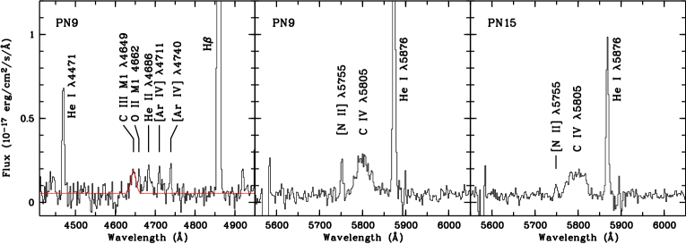
Figure 6.— Spectrum of PN9 and PN15 showing the broad C iv $\lambda$5805 emission line (middle and right panels) of the central stars. The C iii $\lambda$4649 line (left panel) might also be due to the central star emission and is fitted by a Gaussian profile with FWHM $\sim$15 Å.

4. Discussion

4.1. Correlation Studies of Abundances

The abundances of $\alpha$-elements (O, Ne, S, Ar, etc.) of a PN reflect the metallicity ($Z$) of the interstellar medium (ISM) from which the progenitor star of the PN formed. The He/H and N/O ratios are also indicative of progenitor masses: Type I PNe tend to have higher abundance ratios, while Type II PNe generally exhibit low N/O and less massive progenitors (Peimbert, 1978; Maciel, 1992; Kingsburgh & Barlow, 1994). The $\alpha$-elements of PNe also help to constrain the theory of stellar models and probe into the evolution of low- to intermediate-mass stars and consequently chemical evolution of galaxies (e.g., Kwitter & Henry, 2001; Milingo et al., 2002a, b; Kwitter et al., 2003; Henry et al., 2004). Although the exact mechanism(s) still unclear, previous studies of Galactic and Magellanic Cloud PNe have established that PN morphology is a useful indicator of stellar populations (Peimbert & Torres-Peimbert, 1983; Manchado et al., 2000; Shaw et al., 2001; Stanghellini et al., 2002a, b, 2003, 2006). At the distance of M31, all PNe are spatially unresolved, and their central stars cannot be directly observed. The stellar population of PNe can be inferred from the elemental abundances of the nebulae.

Following the discussion in Paper II, in this section we made a correlation study of the abundances of He, N, O and $\alpha$-elements for our extended halo sample (see Figures 7–11). The M31 outer-disk PNe observed by Kwitter et al. (2012), Balick et al. (2013) and Corradi et al. (2015) using large telescopes (Gemini-North and the GTC) were included, and henceforth mentioned as the disk sample (or the disk PNe) in this paper. Also considered in the study were previous observations of PNe and H ii regions in M31, including the bulge and disk PNe from Jacoby & Ciardullo (1999), and the nine H ii regions from Zurita & Bresolin (2012) where the temperature-diagnostic auroral lines were observed. The solar abundances from Asplund et al. (2009) and the abundances of the Orion Nebula from Esteban et al. (2004) were used as benchmarks.

Figure 7 shows the N/O abundance ratio versus He/H (left) and O/H (right) in logarithm. Our sample (the color-filled circles in Figure 7), including the PNe studied in Papers I and II, all have low N/O ($<$0.5) except PN16, a PN associated with M32 and whose N/O ($\sim$1.07$\pm$0.24) is higher than the other targets, and hints at the possibility of Type I nature. Its He/H (=0.114) however, is normal compared to others. Our targets and the disk sample show no obvious trend in N/O versus He/H or O/H, and are clearly separated from the Galactic Type I objects of Milingo et al. (2010), whose N/O seems to be correlated with He/H and anti-correlated with O/H. Among the M31 disk sample, there are two outliers and one of them has N/O close to 1.0. Most of the M31 PNe have higher N/O ratios than H ii regions (including the Orion Nebula), but there are three PNe in our sample with very low N/O. Within our sample, the PNe associated with the Northern Spur, the Giant Stream, and the outer halo generally cannot be distinguished from each other in abundance ratios, although the halo target PN13 has the lowest N/O ratio.

All M31 PNe show positive correlation between neon and oxygen (Figure 8), consistent with the previous observations of PNe in the Galaxy, the Large and Small Magellanic Clouds and M31 (Henry, 1989). One outlier is from Jacoby & Ciardullo (1999). This neon-oxygen positive correlation was defined by the samples of H ii regions and metal-poor blue compact galaxies analyzed by Izotov & Thuan (1999), Izotov et al. (2012) and Kennicutt et al. (2003). We noticed that 12+$\log$(Ne/H) of the Sun (7.93$\pm$0.10, Asplund et al., 2009) is slightly lower than, although still agrees within the errors with, what is expected from the neon-oxygen correlation, indicating that the current solar neon might be underestimated. This problem was investigated through a comparison study of PNe and H ii regions by Wang & Liu (2008).

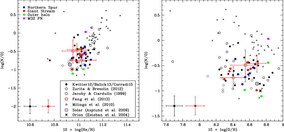
Figure 7.— N/O versus He/H (left) and O/H (right), both displayed in logarithm. Different symbols represent different samples (see the legend). Explanation of different data sets are given in the text. The color-filled (blue, red, green and pink) circles are our GTC sample, including those observed in Paper II; color code is the same as in Figure 1 (see also the top-left legend). Red open circles are the Northern Spur PNe studied in Paper I. The M31 disk PNe observed by Kwitter et al. (2012, Kwitter12), Balick et al. (2013, Balick13) and Corradi et al. (2015, Corradi15) are represented by black filled circles. Typical error bars of the two samples are indicated at the corner. Symbols in Figures 8–11 have the same meaning.

Argon of our targets are generally correlated with oxygen, although the scatter is noticeable (Figure 9). Our sample also seems to have slightly lower argon than what is expected from the argon-oxygen correlation defined by the H ii regions and metal-poor blue compact galaxies, but this deficiency is more obvious in the outer-disk sample, especially in the PNe with lower oxygen [12+$\log$(O/H)$<$8.45]. As discussed in Paper II, sulfur abundances of M31 PNe are all lower than what is expected from the sulfur-oxygen correlation. Although the GTC spectra of four PNe (PN9, PN11, PN13 and PN17) in our sample have covered the [S iii] $\lambda\lambda$9069,9531 lines, their 12+$\log$(S/H) are still underabundant by $\sim$0.24–0.39 dex. This deficiency in sulfur, known as the “sulfur anomaly”, was previously noticed in the Galactic PNe (Henry et al., 2004; Milingo et al., 2010). So far the most plausible explanation seems to be the inadequacy in ICF used to correct for the sulfur ions (e.g., S³⁺ and higher ionization stages) unobserved in the optical but detectable in the IR, although taking into account the IR observations of S³⁺ has alleviated but could not eliminate this deficiency (Henry et al., 2012). Theoretical studies shows that sulfur is unlikely destroyed by the nucleosynthetic processes in the low- to intermediate-mass stars (Shingles & Karakas, 2013). On the other hand, the M31 H ii regions of Zurita & Bresolin (2012) generally agree with the sulfur-oxygen correlation (Figure 10).

Although strictly speaking chlorine cannot be classified as an $\alpha$-element because its two stable isotopes, ³⁵Cl and ³⁷Cl, are not formed through the $\alpha$-processes but produced during both hydrostatic and explosive oxygen burning (Woosley & Weaver, 1995), it is a secondary product during oxygen burning and created from the isotopes of sulfur and argon (Clayton, 2003). Cl/H was derived for five objects in our GTC sample using the [Cl iii] $\lambda\lambda$5517,5537 doublet (Table 6). It has also been derived for three outer-disk PNe. Together with the Galactic samples from Henry et al. (2004, 2010) and Milingo et al. (2010), chlorine exhibits a loose correlation with oxygen (Figure 11). The chlorine-oxygen relation among the M31 PNe alone has large scatter, probably much affected by large uncertainties, given the weakness of the [Cl iii] lines. Using the Galactic H ii regions from Esteban et al. (2015, including the Orion Nebula) as a baseline for correlation, we found that not all M31 PNe are located along this relation within the errors.

4.2. Populations of PNe

In this section, we study the stellar populations of our sample by constraining the central star parameters, which again, were estimated from the observed nebular spectra. In a PN spectrum, the intensities of nebular emission lines, such as [O iii] $\lambda$5007 and He ii $\lambda$4686, relative to the H$\beta$, are to some extent representative of the central star temperature ($T_{\rm eff}$). For an optically thick PN, at a given $T_{\rm eff}$, the central star luminosity ($L_{\ast}$) can be determined from the nebular H$\beta$ luminosity (e.g., Osterbrock & Ferland, 2006). Based on the photoionization models of a large sample of optically thick PNe in the Large and Small Magellanic Clouds (hereafter, LMC and SMC), Dopita & Meatheringham (1991, also ) derived empirical relationships between $T_{\rm eff}$ and $L_{\ast}$ and excitation class (EC) in the form of polynomials (Equations 3.1 and 3.2 in Dopita & Meatheringham 1991). These empirical relations work in equivalent to the transformation between the observed Hertzsprung-Russell (H-R) diagram, $\log{L({\rm H}\beta)}$ versus EC, and the true H-R diagram, $\log{(L_{\ast}/L_{\sun})}$ versus $\log{T_{\rm eff}}$. The EC parameter was defined in terms of the $\lambda$5007/H$\beta$ and $\lambda$4686/H$\beta$ nebular line ratios. However, we were aware that these relationships were based on the models of the optically thick PNe in the Clouds, which are both metal-poor ($Z$=0.008 in the LMC, and 0.004 in the SMC), while previous and our current spectroscopic observations have demonstrated that the bright PNe in the outer-disk and the halo of M31 are all metal-rich (Kwitter et al., 2012; Balick et al., 2013; Fang et al., 2013, 2015; Corradi et al., 2015). The relationships given by Dopita & Meatheringham (1991) could be metallicity dependent (Dopita et al., 1992), although the [O iii]/H$\beta$ line ratio is less dependent than other lines. Thus whether they are applicable to the PNe in M31 might be questionable.

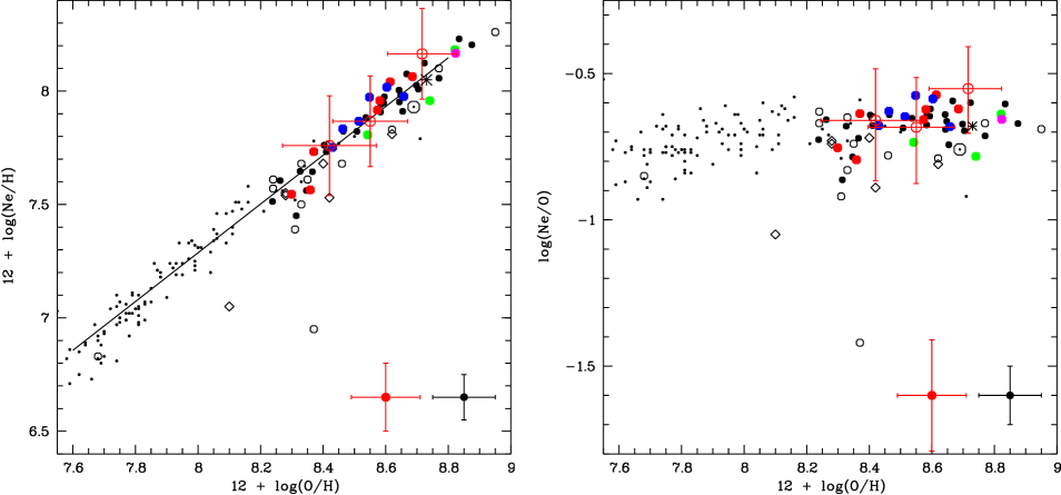
Figure 8.— Ne/H versus O/H (left) and Ne/O versus O/H (right), both displayed in logarithm. The small black dots are the extragalactic H ii regions and metal-poor blue compact galaxies (see references in the text), and the solid black line in the left panel is a least-squares linear fit to these data. These symbols in Figures 9 and 10 have the same meaning. Color codes of the other symbols are the same as in Figure 7.

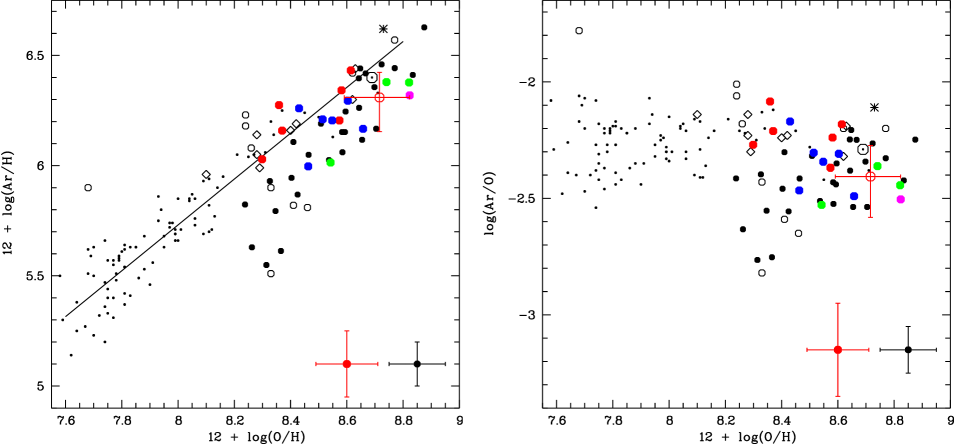
Figure 9.— Same as Figure 8 but for Ar/H versus O/H (left) and the Ar/O ratio versus O/H (right).

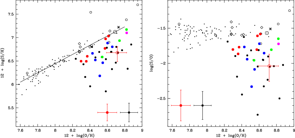
Figure 10.— Same as Figure 8 but for S/H versus O/H (left) and the S/O ratio versus O/H (right).

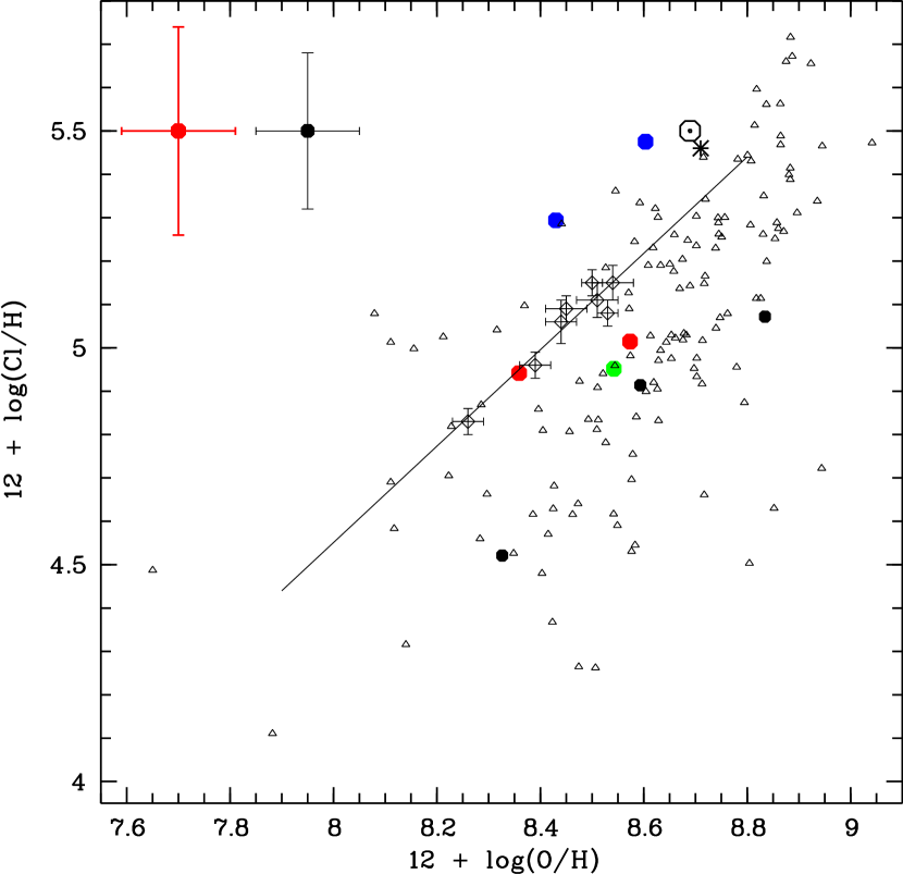
Figure 11.— The Cl/H versus O/H in logarithm scale. The small open triangles are the Galactic PN samples from Henry et al. (2004, 2010) and Milingo et al. (2010); the open diamonds are the Galactic H ii regions studied by Esteban et al. (2015), and the black line is a linear fit to this sample, with a slop of 1.11$\pm$0.15. The other symbols and color codes are the same as in Figure 7.

In order to assess the applicability of the relationship of Dopita & Meatheringham (1991), we derived the $T_{\rm eff}$ for the M31 disk PNe studied by Kwitter et al. (2012) and Balick et al. (2013) using the relation, and compared them with the cloudy model results presented in these two papers. The differences in $\log{T_{\rm eff}}$ are mostly less than 0.06 dex. We made the same comparison of the $L_{\ast}$ of the same disk sample, and found that the differences in $\log{(L_{\ast}/L_{\sun})}$ are mostly less than 0.05 dex. The disk sample contains the brightest PNe in M31 with $m_{\lambda 5007}\sim$20.4–20.9. This comparison study between the two sets of $T_{\rm eff}$ and $L_{\ast}$ thus confirms our anticipation that the brightest PNe in M31, those within two magnitudes from the bright cut-off of the PNLF, should not be quite evolved and probably still optically thick (A. A. Zijlstra, private communications). We noticed that the empirically derived $L_{\ast}$ of three less bright PNe (with $m_{\lambda 5007}$ = 20.72, 20.88 and 20.89) are lower than their corresponding cloudy models by $\sim$0.2 dex. This difference might be due to a possibility that the empirical relationship of Dopita & Meatheringham (1991) underestimates the stellar luminosities of fainter PNe, which might no longer be optically thick. We made a similar comparison study of the stellar parameters for the M31 bulge and disk PNe of Jacoby & Ciardullo (1999), which are systematically fainter ($m_{\lambda 5007}\sim$20.73–23.16), and found that the empirically derived $\log{(L_{\ast}/L_{\sun})}$ are lower than the photoionization models by 0.2 dex in average (although scatter in the sample of Jacoby & Ciardullo 1999 is large due to faintness of the targets). The largest difference in both $\log{T_{\rm eff}}$ and $\log{(L_{\ast}/L_{\sun})}$ is found in the brightest PN of Balick et al. (2013, PN ID M2496, $m_{\lambda 5007}$ =20.42).

Table 9Estimated Properties of PN Central Stars and the Progenitors^a

			$Z$=0.016 b			$Z$=0.01 c			$Z$=0.02 c
ID	$\log{T_{\rm eff}}$	$\log{(L_{\ast}/L_{\sun})}$	$M_{\rm fin}$	$M_{\rm ini}$	$t_{\rm ms}$	$M_{\rm fin}$	$M_{\rm ini}$	$t_{\rm ms}$	$M_{\rm fin}$	$M_{\rm ini}$	$t_{\rm ms}$
PN1	4.971	3.657	0.597	1.82	1.43	0.563	1.53	1.77	0.565	1.55	2.32
			$\cdots$	1.75	1.61	$\cdots$	1.40	2.31	$\cdots$	1.42	3.05
PN2	5.077	3.464	0.594	1.80	1.49	0.556	1.47	1.99	0.554	1.45	2.82
			$\cdots$	1.72	1.69	$\cdots$	1.32	2.71	$\cdots$	1.30	3.99
PN3	5.126	3.696	0.618	2.00	1.10	0.583	1.70	1.31	0.579	1.67	1.85
			$\cdots$	1.97	1.15	$\cdots$	1.60	1.55	$\cdots$	1.56	2.25
PN4	4.932	3.525	0.576	1.64	1.94	0.550	1.42	2.20	0.545	1.38	3.35
			$\cdots$	1.53	2.40	$\cdots$	1.26	3.13	$\cdots$	1.21	5.08
PN5	5.052	3.702	0.606	1.90	1.27	0.576	1.64	1.44	0.577	1.65	1.91
			$\cdots$	1.84	1.38	$\cdots$	1.53	1.76	$\cdots$	1.54	2.34
PN6	4.989	3.448	0.597	1.82	1.43	0.563	1.53	1.77	0.565	1.55	2.32
			$\cdots$	1.75	1.61	$\cdots$	1.40	2.31	$\cdots$	1.42	3.05
PN7	4.967	3.445	0.570	1.59	2.14	0.545	1.38	2.41	0.539	1.32	3.78
			$\cdots$	1.47	2.73	$\cdots$	1.21	3.55	$\cdots$	1.15	6.04
PN8	5.082	3.310	0.585	1.72	1.69	0.559	1.50	1.89	0.559	1.50	2.57
			$\cdots$	1.62	2.00	$\cdots$	1.35	2.53	$\cdots$	1.35	3.52
PN9	5.073	3.501	0.589	1.76	1.60	0.558	1.49	1.92	0.558	1.49	2.62
			$\cdots$	1.67	1.85	$\cdots$	1.34	2.59	$\cdots$	1.34	3.61
PN10	4.980	3.687	0.602	1.87	1.34	0.567	1.56	1.66	0.570	1.59	2.13
			$\cdots$	1.80	1.47	$\cdots$	1.44	2.12	$\cdots$	1.47	2.72
PN11	5.137	3.662	0.611	1.94	1.20	0.583	1.70	1.31	0.578	1.66	1.88
			$\cdots$	1.90	1.28	$\cdots$	1.60	1.55	$\cdots$	1.55	2.29
PN12	4.761	3.639	0.584	1.71	1.72	0.554	1.45	2.06	0.553	1.44	2.87
			$\cdots$	1.61	2.04	$\cdots$	1.30	2.84	$\cdots$	1.29	4.10
PN13	4.906	3.423	0.567	1.57	2.24	0.536	1.30	2.86	0.530	1.25	4.58
			$\cdots$	1.44	2.92	$\cdots$	1.11	4.52	$\cdots$	1.05	7.96
PN14	4.825	3.643	0.588	1.75	1.62	0.556	1.47	1.98	0.555	1.46	2.76
			$\cdots$	1.66	1.89	$\cdots$	1.32	2.71	$\cdots$	1.31	3.89
PN15	5.067	3.380	0.580	1.68	1.83	0.551	1.43	2.16	0.546	1.38	3.28
			$\cdots$	1.57	2.21	$\cdots$	1.27	3.05	$\cdots$	1.22	4.94
PN16	5.240	3.331	0.633	2.13	0.93	0.583	1.70	1.31	0.579	1.67	1.85
			$\cdots$	2.12	0.94	$\cdots$	1.60	1.54	$\cdots$	1.56	2.25
PN17	5.166	3.464	0.610	1.93	1.21	0.574	1.62	1.49	0.576	1.64	1.94
			$\cdots$	1.88	1.30	$\cdots$	1.51	1.84	$\cdots$	1.53	2.39
NOTE. – All masses are in unit of solar mass ($M_{\sun}$) and ages in giga years (Gyr).

^a

For each PN, $M_{\rm ini}$ values in the first and second lines were derived using Equations 1 and 2 of the linear initial-final mass relations of Catalán et al. (2008), respectively. $t_{\rm ms}$ was derived based on the model grids computed by Schaller et al. (1992).

^b

$M_{\rm fin}$ were interpolated from the post-AGB model tracks of Vassiliadis & Wood (1994).

^c

$M_{\rm fin}$ were interpolated from the post-AGB model tracks of Miller Bertolami (2016).

The EC of our target PNe are mostly between $\sim$3 and 7.6. We derived their central star temperatures and luminosities using the relationships of Dopita & Meatheringham (1991). Despite the applicability of these relationships assessed above, the stellar luminosity thus derived might still be underestimated for 1) bright, young (and thus probably dusty) PNe due to absorption of a large fraction of stellar flux by dust, and 2) the PNe that are optically thin to the ionizing radiation of the central stars. Since the extinction of our targets are low (Section 3.1), the first possibility could be discounted. The relatively faint PNe in M31 might not be optically thick, and their stellar luminosities derived using the empirical relationship might be underestimated. According to the discussion above, we revised up the $\log{(L_{\ast}/L_{\sun})}$ of the fainter targets ($m_{\lambda 5007}\geq$21) in our sample by 0.2 dex to compensate for the possible underestimation. The stellar temperatures and luminosities of our PNe are presented in Table 9 (the second and third columns).

The model-based $\log{(L_{\ast}/L_{\sun})}$ versus EC relation of Dopita & Meatheringham (1991) actually is similar to the method of Zijlstra & Pottasch (1989), who derived the central star luminosities of PNe using the H$\beta$ flux only. With the assumption that PNe are optically thick to the ionizing stellar radiation, the methodology of Zijlstra & Pottasch (1989) is analogous to the Zanstra method for determining stellar temperatures (Zanstra, 1931). This assumption is justified by the very high optical depth of the H i Lyman emission lines: each recombination of hydrogen (H⁺ + e^-) eventually results in emission of Balmer lines and the Ly$\alpha$ photon (Osterbrock & Ferland, 2006). Following the method of Zijlstra & Pottasch (1989) and the tabulation of $T_{\rm eff}$ versus $L_{\ast}$ in Pottasch (1984, p.169), we derived the stellar luminosities that are close to those derived using the empirical relationship of Dopita & Meatheringham (1991).

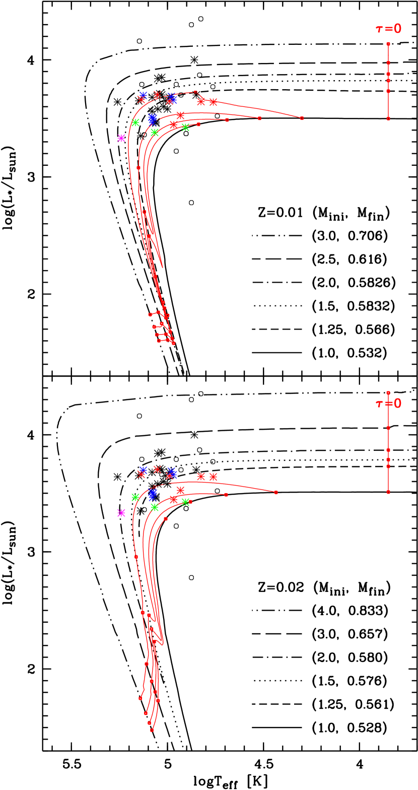
Figure 12.— Central star positions of M31 PNe in the $\log{(L_{\ast}/L_{\sun})}$ vs. $\log{T_{\rm eff}}$ diagram. The black asterisks are the disk PNe observed by Kwitter et al. (2012) and Balick et al. (2013); our targets are represented by the colored asterisks (color codes are the same as in previous figures). The black open circles are the M31 bulge and disk PNe studied by Jacoby & Ciardullo (1999). Over-plotted in the diagram are the model tracks of the H-burning post-AGB sequences calculated by Miller Bertolami (2016) at $Z$=0.01 (top) and 0.02 (bottom); different line types represent different initial and final masses. Red curves are isochrones for the evolutionary ages ($\tau$ = 0, 5000, 10 000, 15 000, and 20 000 yr) since the zero point of post-AGB defined at $\log{T_{\rm eff}}$ =3.85.

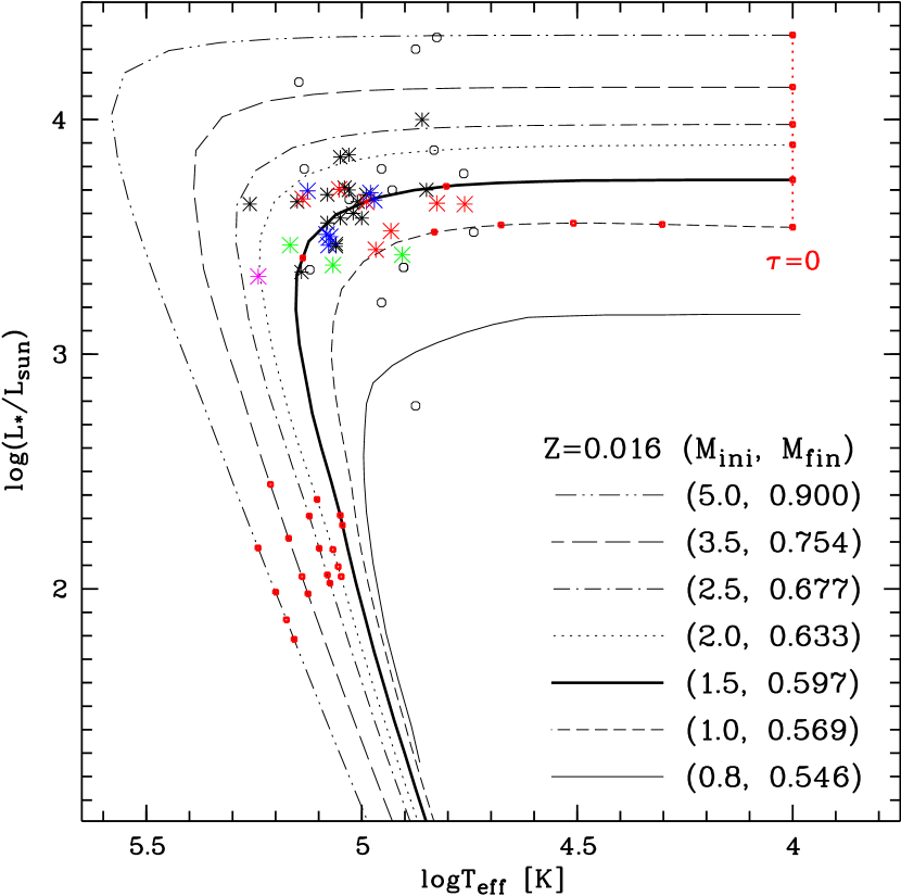
Figure 13.— Same as Figure 14 but over-plotted with the H-burning post-AGB evolutionary models of Vassiliadis & Wood (1994, $Z$=0.016). The model track with 0.546 $M_{\sun}$ core mass is adopted from Schönberner (1983). Red dots on the model tracks have the same meaning as in Figure 12.

The $\log{T_{\rm eff}}$ versus EC relation of Dopita & Meatheringham (1991) is dependent on the spectral energy distribution (SED) of the ionizing source. Blackbodies (i.e., Planck function), as assumed in the photoionization models of Dopita & Meatheringham (1991), can result in different $\log{T_{\rm eff}}$ versus EC relations from the cases where more realistic models (like those of Rauch 2003) are used. At a given intensity ratio of two nebular lines, e.g., $I$(He ii $\lambda$4686)/$I$(H$\beta$), the stellar atmospheres of Rauch (2003) can predict higher $T_{\rm eff}$ than does a blackbody. In this regard, we tried to constrain the central star temperatures and luminosities by fitting the observed line ratios (including $\lambda$4363/$\lambda$5007, He i/He ii, [O ii]/[O iii], [Ar iii]/[Ar iv], [Ne iii]/[O iii], and [S ii]/[S iii]) to those predicted by the photoionization models calculated at a huge number of grids, the Mexican Million Models dataBase (3MdB, Morisset et al., 2015). The 3MdB models were computed with the cloudy program (Ferland et al., 2013) and include both the radiation- and the matter-bounded cases, as well as stellar SEDs of both blackbody and Rauch’s atmospheres. The tolerance of fitting was set to be $\leq$20% for all line ratios. Using the 3MdB, we managed to obtain $T_{\rm eff}$ for nine objects in our sample, and they generally agree within the errors with the corresponding values derived using the empirical relationship of Dopita & Meatheringham (1991). However, no optimum constraint on stellar luminosity was achieved.

The emergent spectrum of a PN can be affected by many factors, including central star parameters ($T_{\rm eff}$, $L_{\ast}$, $\log{g}$), density profile of the nebular shell, nebular abundances, nebular radius, and filling factor; fixing other parameters and varying only $T_{\rm eff}$ and $L_{\ast}$, as was usually done with cloudy for extragalactic PNe, could be unrealistic and the derived parameters problematic. In particular, determining the central star luminosity without knowing the exact covering factor ($\leq$1) of the nebula may underestimate $L_{\ast}$, not mentioning the case where the nebula is optically thin.

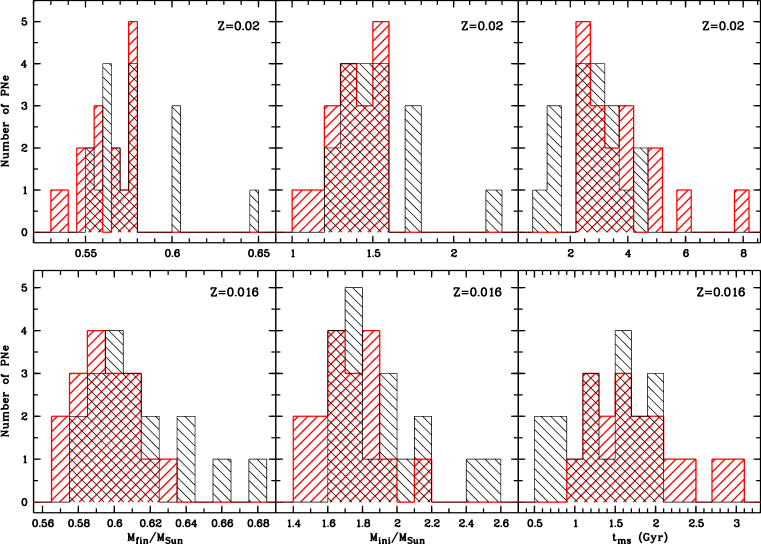
Figure 14.— Number distributions of the core masses ($M_{\rm fin}$, left), initial masses ($M_{\rm ini}$, middle) and main-sequence ages ($t_{\rm ms}$, right) of M31 PNe derived using the post-AGB evolutionary models of Miller Bertolami (2016, $Z$=0.02; top panels) and Vassiliadis & Wood (1994, $Z$=0.016; bottom panels). $M_{\rm ini}$ were derived using the Equation 2 of Catalán et al. (2008). Derivation of $t_{\rm ms}$ is described in the text. The red-shaded histograms represent our sample, and the black-shaded histograms the disk sample.

The central star locations of our PNe in the H-R diagram are shown in Figure 12, along with the new model tracks of the H-burning post-asymptotic giant branch (post-AGB) evolutionary sequences calculated by Miller Bertomali (2015, 2016) at two metallicities, $Z$=0.01 and 0.02, for various initial masses. These two metallicities were chosen for analysis because they bracket the solar metallicity ($Z_{\sun}\sim$0.013–0.018, Grevesse & Noels, 1993; Grevesse & Sauval, 1998; Lodders, 2003; Asplund et al., 2009) and thus are probably suitable for the metallicity environment of M31 (as discussed in Section 4.3, the O/H ratios of the total sample of M31 PNe are mostly located between the AGB models with $Z$=0.007 and 0.019). Also over-plotted in the H-R diagram are the 18 M31 disk PNe observed by Kwitter et al. (2012, 16 PNe) and Balick et al. (2013, two PNe). Our targets are located between the model tracks with 0.53–0.58 $M_{\sun}$ final masses, while the disk sample are mostly 0.56–0.657 $M_{\sun}$, with a few objects extending to $<$0.56 $M_{\sun}$ (Figure 12, bottom). The 15 disk and bulge PNe from Jacoby & Ciardullo (1999) are also presented in Figure 12, but with large scatter in stellar luminosity. In order to make a contrast study, we also placed all samples in Figure 13 where the classical/old post-AGB evolutionary model tracks of Vassiliadis & Wood (1994) are presented.

The final core masses ($M_{\rm fin}$) of our targets and the M31 disk sample were interpolated from the model tracks. Our targets, as constrained by the new post-AGB models, are in the range 0.536–0.583 $M_{\sun}$ (Table 9) with an average mass of 0.562($\pm$0.015) $M_{\sun}$, while the disk sample are mostly 0.550–0.602 $M_{\sun}$ with an average of 0.571($\pm$0.016) $M_{\sun}$. Based on the old models, the core masses of our sample are 0.567–0.633 $M_{\sun}$, and the disk PNe are $\sim$0.583–0.660 $M_{\sun}$. The initial masses ($M_{\rm ini}$) were then derived using the semi-empirical initial-final mass relation (IFMR) of white dwarfs given by Catalán et al. (2008). A comparison between the core masses derived for the two samples using the two sets of post-AGB models is presented in Figure 14 (left).

Previously, Kwitter et al. (2012) derived the $M_{\rm ini}$ of their disk sample using Equation 1 in Catalán et al. (2008), which is a single linear fit to the IFMR in the 1–6 $M_{\sun}$ range. In order to make a comparison study with the disk sample, we also adopted this equation for our sample. However, in the low-mass range (1–2 $M_{\sun}$), the actual IFMR seems to be flatter than what the usual semi-empirical linear fits predict (Salaris et al., 2009; Gesicki et al., 2014). Given that our targets seem to be located between the post-AGB evolutionary tracks with the 1 and 2 $M_{\sun}$ initial masses, we also derived the $M_{\rm ini}$ using Equation 2 of Catalán et al. (2008), which is a linear fit for the $<$2.7 $M_{\sun}$ range and is expected to better describe the IFMR at low masses. The $M_{\rm ini}$ thus derived are also presented in Table 9 along with those derived using Equation 1 of Catalán et al. (2008). The main-sequence lifetimes ($t_{\rm ms}$) were then derived from $M_{\rm ini}$ based on the stellar model grids computed by Schaller et al. (1992, Tables 45 and 46 therein).

Our targets extend to lower core mass regions than the disk sample in the H-R diagram, and consequently older main-sequence stellar ages. Compared to the old post-AGB evolutionary models, the new models of Miller Bertolami (2016) have lowered the core masses and shortened the post-AGB evolutionary timescales. Using the new models, we estimated the initial masses of the brightest PNe in our sample (PN9, PN10, PN11 and PN16), whose [O iii] luminosities are within 1 magnitude from the PNLF bright cut-off (Merrett et al., 2006), to be $\sim$1.3–1.6 $M_{\sun}$. This hints at a tantalizing possibility that the brightest PNe may also evolve from very low-mass stars. Figure 14 compares the initial masses and main-sequence stellar ages of the two samples of M31 PNe that were derived based on the two sets of post-AGB evolutionary models. It is noteworthy that according to the new post-AGB models, our sample 1) extends to core mass as low as 0.53 $M_{\sun}$ (Figure 14, top-left), below the lower mass limit (0.55 $M_{\sun}$) for the formation of PNe predicted by the old models, and 2) may evolved from young ($\sim$2 Gyr) to intermediate age ($\sim$6–8 Gyr) stars (while the old models place our targets in the young population, $\lesssim$3 Gyr).

Within our sample, we did not find obvious systematic difference in stellar mass or main-sequence age between the groups of PNe associated with different regions, although the three halo PNe (PN13, PN15 and PN17) seem to have lower stellar luminosities. According to the old stellar models, a post-AGB system with core mass lower than 0.55 $M_{\sun}$ is unable to develop a visible PN because its transition time (from the beginning of post-AGB to the PN phase) is too long for the star to become hot enough ($\gtrsim$30 000 K) to ionize the ever-expanding nebular shell (e.g., Schönberner, 1983). Updated micro- and macro-physics have been included in the new post-AGB models of Miller Bertolami (2016), which predict higher central star luminosities than the earlier models of Vassiliadis & Wood (1994, also and ) by $\sim$0.1–0.3 dex at given core masses, and have accelerated the post-AGB evolution by a factor of 3 to 8, enabling formation of PNe with core masses as low as $\sim$0.53 $M_{\sun}$. This acceleration in post-AGB evolution, which was previously proposed for the existing Blöcker (1995) model tracks by Gesicki et al. (2014) and has been well confirmed by a recent study of the central stars of 32 Galactic bulge PNe (Gesicki et al., 2017; Zijlstra et al., 2017), is more significant at lower core masses, which is reflected in that the post-AGB timescales predicted by the new models are extremely sensitive to core mass, making the low-mass PN central stars much more abundant than the more massive ones.

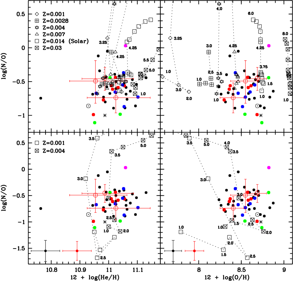
Figure 15.— The N/O versus the He/H (left) and O/H (right) abundance ratios (in logarithm); only our targets and the M31 disk sample are presented, along with the abundance ratios of the sun (Asplund et al., 2009) and the Orion Nebula (Esteban et al., 2004). Symbols and color codes are the same as in Figure 7. In the top panels: AGB model predictions from Karakas (2010, $Z$=0.004), Fishlock et al. (2014, $Z$=0.001) and Karakas & Lugaro (2016, $Z$=0.007, 0.014 and 0.03) for the surface abundances at different metallicities are over-plotted for purpose of comparison. In the bottom panels: AGB model predictions from Ventura et al. (2013, $Z$=0.001) and Ventura et al. (2014, $Z$=0.004) are over-plotted. Different symbols represent different metallicities; symbols of the same metallicity are linked by dotted lines to aid visualization. Initial mass (in $M_{\sun}$) of the progenitor star is labeled for each model. The vertical scales of the top and bottom panels are different to accommodate the AGB model grids.

Most of the PNe in our sample are located before the 10 000 yr isochrone (i.e., the post-AGB evolution ages) (Figure 12). This distribution in the H-R diagram is qualitatively in line with the fact that these bright M31 PNe should not be quite evolved so that they can still be observed today. A considerable fraction of the disk PNe are located before the 5000 yr isochrone; this does not necessarily mean that they are very young PNe but might be due to overestimated stellar luminosities. In a similar sense, for those PNe located after the 10 000 yr isochrones, their stellar luminosities might be underestimated. In overall, the locations of our sample of M31 PNe in the H-R diagram are reasonable.

4.3. Comparison with AGB Model Predictions

The chemical yields of an AGB star are on dependent on its initial mass and metallicity ($Z$). For an AGB star with $M_{\rm ini}\sim$0.8–8 $M_{\sun}$, its surface abundances can be altered due to recurrent mixing events that bring the synthesized material to the surface (c.f., reviews Herwig 2005; Karakas & Lattanzio 2014). For stars with $M_{\rm ini}\gtrsim$1.25 $M_{\sun}$, in the thermally pulsing AGB phase, instabilities in the thin He-burning shell will drive the third dredge-up, which brings the material from He-intershell and enriches the surface with carbon and $s$-process elements (e.g., Herwig, 2005). Depending on $Z$, AGB stars with $M_{\rm ini}\geq$3–4$\,M_{\sun}$ experience the second dredge-up and hot bottom burning (HBB), which results in a significant increase in the surface nitrogen at the expense of carbon and oxygen (e.g., Karakas, 2010). The nebular relative elemental abundances are thus indicative of $M_{\rm ini}$ and $Z$. Analysis of observations against theoretical predictions provides insights to stellar astrophysics as well as assessment of the stellar evolution models. A number of theoretical efforts have been made to investigate stellar yields from AGB nucleosynthesis for various cases of $M_{\rm ini}$ and $Z$ (e.g., Herwig, 2005; Karakas et al., 2009, 2014; Karakas, 2010; Cristallo et al., 2011, 2015; Lugaro et al., 2012; Ventura et al., 2013, 2014; Fishlock et al., 2014; Shingles et al., 2015; Karakas & Lugaro, 2016; Pignatari et al., 2016). In this section, we make a comparison study between the elemental abundances of M31 PNe, as derived from deep spectroscopy, and AGB model predictions, aiming at constraining the initial stellar masses and investigating the dependence of stellar yields on the mass.

In Figures 15 and 16 we compare the He/H, O/H, N/O and Ne/H abundance ratios of M31 PNe to those predicted by the AGB nucleosynthesis models at different metallicities and initial stellar masses. The PN samples include our PNe (this work and Papers I and II), most of which are associated with substructures, and the disk sample observed by Kwitter et al. (2012, also and ). Sources of the AGB models are given in the caption of Figure 15, and cover a broad range of metallicity ($Z$=0.001–0.03). The He/H and O/H ratios of most PNe are located between the AGB models with $Z$=0.004 (SMC) and 0.014 ($\sim$solar), although the model yields of Karakas et al. are insensitive to stellar mass at $\leq$3 $M_{\sun}$; there seems to be a few objects with slightly over-solar oxygen, but still consistent with the Sun within the errors. In the AGB models of Karakas et al., N/O was assumed to be solar. Depending on the initial mass, all mixing events during the evolution of a low- to intermediate-mass star increase nitrogen by a certain amount. However, the model predicted N/O of Karakas et al. does not extend to such low levels as observed in our PN targets (Figure 15, top). It is unlikely that these AGB models over-predict N/O, given that 1) the N/O ratio only depends on the first dredge-up (because all PNe in our sample probably correspond to progenitors with $M_{\rm ini}\lesssim$2 $M_{\sun}$) and 2) for the low-mass AGB models, predictions for the first dredge-up more or less all agree. Thus we conclude that several objects in our sample (as well as the disk sample) were probably born in the ISM with very low N/O ratios.

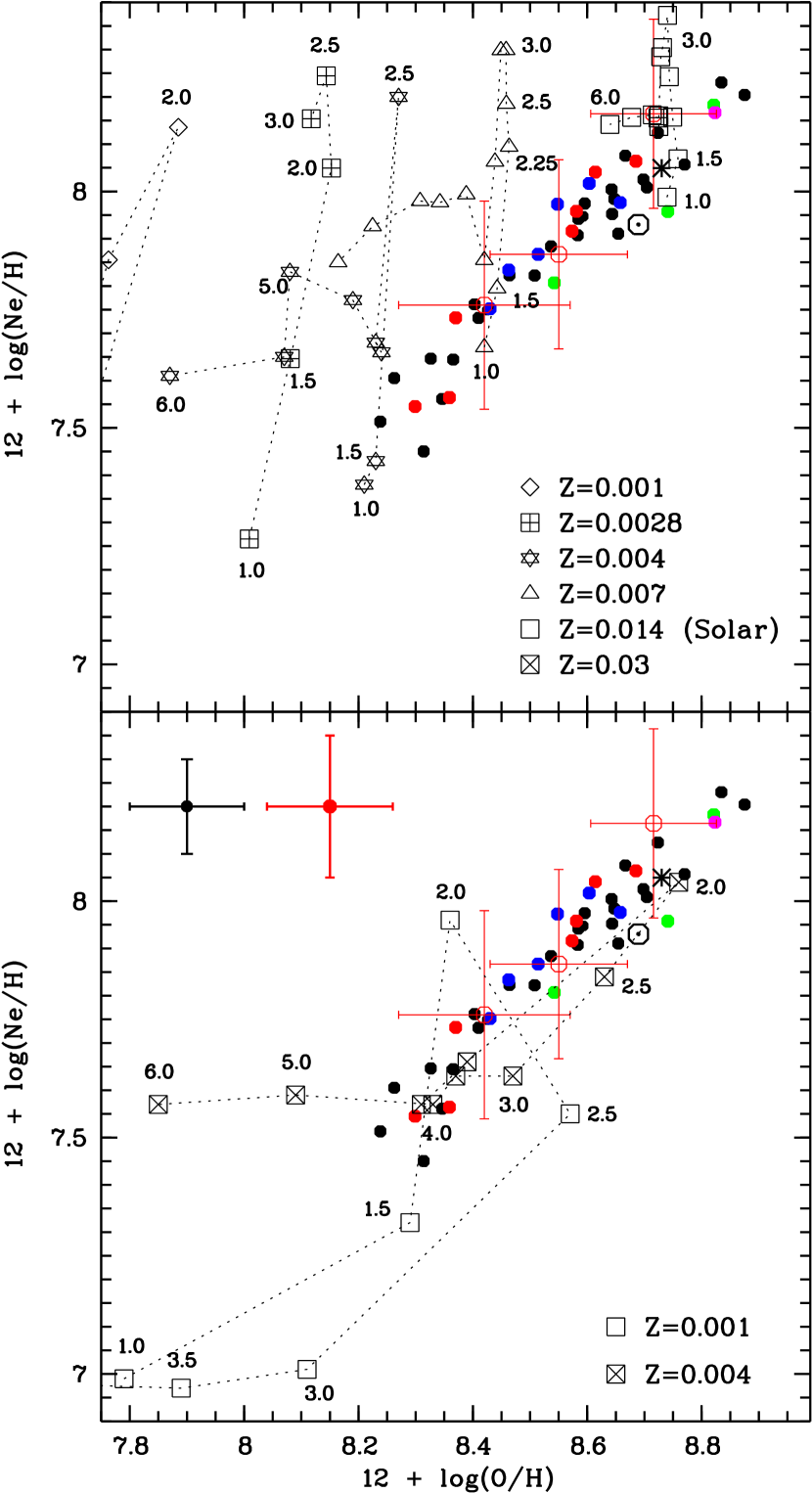
Figure 16.— Same as Figure 15 but for Ne/H versus O/H.

By contrast, N/O predicted by the AGB models of Ventura et al. (2013, 2014) is very sensitive to the initial stellar mass (Figure 15, bottom). Besides, their model-predicted N/O ratios also extend to as low as 0.02 (i.e., $\log$(N/O)=$-$1.68). These differences are mainly due to the different initial compositions adopted in the two set of models, although prescriptions for convection are also different – the third dredge-up and HBB were considered at a lower stellar mass in Ventura’s models ($\sim$3 $M_{\sun}$) than in the models of Karakas et al. ($\gtrsim$4–5 $M_{\sun}$). The initial stellar masses of the M31 PNe can mostly be constrained by Ventura’s models to be $\lesssim$3 $M_{\sun}$, consistent with the estimate of Kwitter et al. (2012, also ). The two sets of AGB models thus generally constrain the M31 PNe in metallicity and place an upper-limit on their initial masses. Ventura’s AGB models also predict higher O/H at given metallicities and stellar masses, mainly due to the inclusion of convective boundary mixing (or overshooting) at different stellar evolutionary stages, especially at the thermally pulsing AGB (TP-AGB) phase, of their models that leads to the dredge up of oxygen to the surface. The broad range of $Z$ (0.004–0.014) in M31 PNe can also be seen in the $\log$(Ne/H) versus $\log$(O/H) diagram (Figure 16).

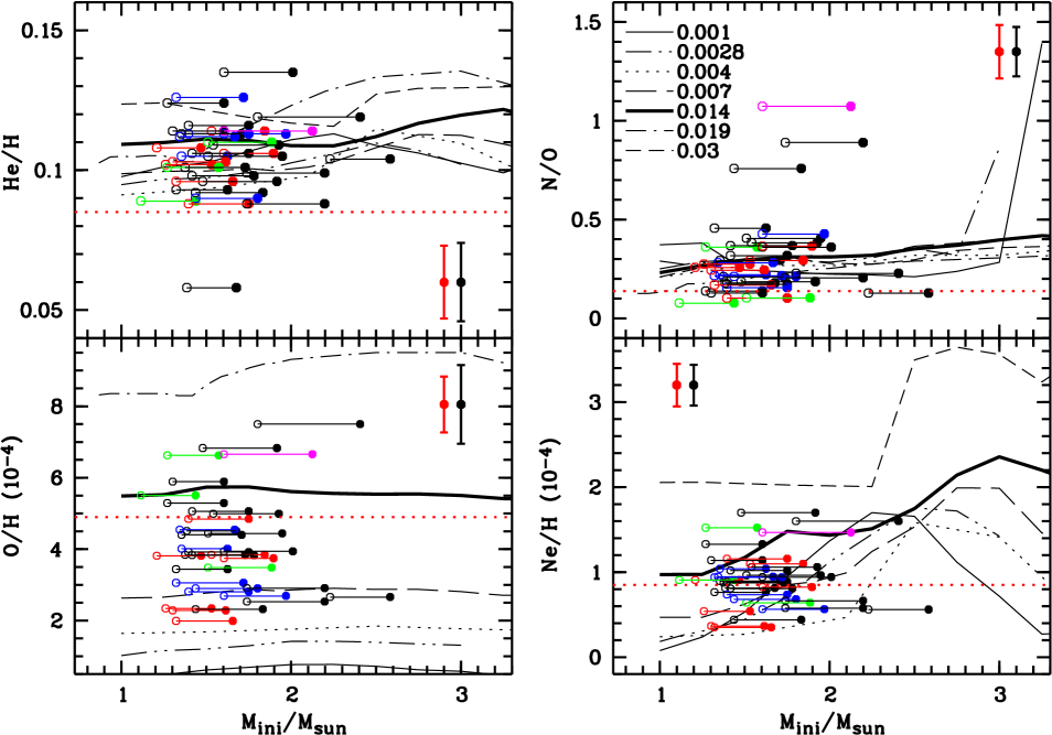
Figure 17.— Abundance ratios of M31 PNe versus initial mass. Sample includes our targets and the disk PNe from Kwitter et al. (2012) and Balick et al. (2013). For each PN, the initial masses derived from the post-AGB evolutionary models of Vassiliadis & Wood (1994, filled circle) and Miller Bertolami (2016, open circle) are both presented and connected by a solid line. Color codes of data points are the same as in Figures 15 and 16. Representative abundance errors of the two samples are indicated. The AGB yields predicted at different metallicities, as represented by different line types (see the legend), are over-plotted. The AGB models are from Karakas (2010, $Z$=0.004), Fishlock et al. (2014, $Z$=0.001), Karakas & Lugaro (2016, $Z$=0.007, 0.014 and 0.03), and Marigo (2001, $Z$=0.019). The horizontal red-dotted lines mark the solar values (Asplund et al., 2009).

Using the initial masses of the total sample of M31 PNe estimated in Section 4.2, we demonstrate the dependence of abundance ratios on $M_{\rm ini}$ in Figure 17. The AGB model predictions presented in the top panels of Figures 15 and 16 are also used in Figure 17. The theoretical AGB yields from Marigo (2001) at $Z$=0.019 are also included. The $M_{\rm ini}$ were those derived using the linear fit to the IFMR at low-masses given by Catalán et al. (2008, Equation 2 therein). For each PN, the initial masses derived based on the old post-AGB evolutionary models of Vassiliadis & Wood (1994) and the new models of Miller Bertolami (2016) were both presented. Generally, the abundance ratios of our targets and majority of the disk sample agree within the uncertainties with the theoretical AGB yields at given stellar masses. In the disk sample, there is an “outlier” with very low He/H, probably due to large uncertainty in the observations (Kwitter et al., 2012).

Interestingly, there is no obvious difference in the O/H ratios between our halo sample and the outer-disk sample, although the initial stellar masses of the disk PNe seem to be higher than those of our targets at given O/H. The O/H ratios of both samples of M31 PNe are located between the AGB models with $Z$=0.004 and 0.019 (Figure 17, bottom-left); these two $Z$ values correspond to [Fe/H]$\sim-$0.5 and $\sim$0.1, respectively, generally metal-rich compared to the halo metallicities of M31 (Ibata et al., 2007, 2014). Given that oxygen is the best observed element in PNe and has been used as a proxy for the metallicity of progenitor stars, from which oxygen is assumed to be inherited, this distribution of the observed O/H with respect to the AGB model predictions confirms the metal-rich nature of these M31 PNe. The insensitivity of the model-predicted N/O on stellar mass at low masses, as predicted by the AGB models of Karakas et al. (Figure 15, top), is better seen in Figure 17 (top-right). This is because the first dredge-up that occurs in AGB stars with $M_{\rm ini}\leq$3–4 $M_{\sun}$ does not increase nitrogen much, and oxygen is essentially unchanged. Figure 17 (top-right) also shows that significant increase in N/O occurs at $M_{\rm ini}>$3 $M_{\sun}$ for the metal-poor case $Z$=0.001; in the metal-rich AGB stars (e.g., $Z$=0.014), N/O increases significantly for $M_{\rm ini}\geq$4 $M_{\sun}$ (Karakas & Lugaro, 2016). The M31 PNe discussed in this paper mostly have initial masses $\lesssim$2 $M_{\sun}$. The dispersion in Ne/H of the total sample is much smaller than that in O/H, with an average ratio of 8.64($\pm$3.35)$\times$10^-5 for our sample and 9.47($\pm$3.34)$\times$10^-5 for the disk sample. Abundances of the PNe are mostly consistent with the AGB model predictions within the errors.

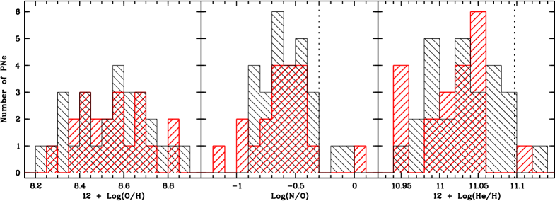
Figure 18.— Histograms of M31 PNe in the O/H (left), N/O (middle) and He/H (right) ratios in logarithm. The red-shaded histograms represent our sample, and the black-shaded histograms the disk PNe. The vertical dotted lines mark the original definition of Galactic Type I PNe by Peimbert & Torres-Peimbert (1983): N/O$>$0.5 or He/H$>$0.125.

Looking at the initial masses derived from the old post-AGB evolutionary models, the N/O ratio seems to start to increase at $M_{\rm ini}$ close to 2 $M_{\sun}$ (Figure 17, top-right). This trend is shifted to lower masses when the new post-AGB models are used. A similar behavior in N/O has also been found in a recent study of the Galactic PNe (Henry et al., 2018). This is at variance with the current AGB model prediction that N/O increases as a consequence of HBB at $M_{\rm ini}\gtrsim$3–5 $M_{\sun}$ (Cristallo et al., 2011, 2015; Karakas et al., 2014; Karakas & Lugaro, 2016; Ventura et al., 2015; Di Criscienzo et al., 2016), and tentatively implies HBB might actually occur at $M_{\rm ini}<$3 $M_{\sun}$, or even at $\lesssim$2 $M_{\sun}$. More detailed investigation is needed to assess this possibility.

There are three PNe with N/O$>$0.5 (a criterion to define the Galactic Type I PNe): PN5 and PN16 from the disk sample of Kwitter et al. (2012), and target PN16 in our sample. However, the He/H ratios of the three PNe are $<$0.125, at odds with the definition of a Type I PN. The initial stellar masses of the three PNe are all $\lesssim$2.2 $M_{\sun}$ (Figure 17, top-right). Apart from the convective mixing processes (mostly the first dredge-up for low-mass stars), N/O in stars with initial masses of 1–4 $M_{\sun}$ may also be affected by the non-standard mixing processes such as thermohaline mixing and stellar rotation (Karakas et al., 2009). This means that AGB stars with high N/O ratios may not necessarily have evolved from the intermediate-mass (3–8 $M_{\sun}$) stars, where HBB is needed to enhance the surface nitrogen, but from low-mass (1–3 $M_{\sun}$) stars that rotate reasonably rapidly on the main sequence and/or experience non-convective mixing processes during the ascent of the first giant branch. However, to what extent N/O can be affected by the thermohaline mixing, especially for the low-mass stars, is still unclear. So far very few stellar evolution models have included thermohaline mixing and rotation (e.g., Charbonnel & Lagarde, 2010; Cantiello & Langer, 2010). More detailed and quantitative investigation of the effects of these extra-mixing processes on the chemical yields of low-mass stars is still needed.

It is worth to mention that the solar abundances quoted in this paper are photospheric values (Asplund et al., 2009, Table 1 therein), which differ slightly from the initial abundances (or the bulk abundances; Asplund et al. 2009, Table 5 therein) due to the combined effects of gravitational settling and diffusion. When the Sun becomes a red giant, its photospheric abundances will go back to the bulk values because of convective mixing. During the post-main sequence evolution, the first and third dredge-ups change the abundances of the Sun. Stellar evolution models of low-mass (1–2 $M_{\sun}$) stars predict that helium of the Sun can be increased by $\sim$0.05 dex, and N/O increased by nearly 0.3 dex (Miller Bertolami, 2016). Thus the actual locations of the Sun in Figures 15, 16 and 17 (also Figures 7) should be more consistent with the M31 PNe than what they appear to be now.

Finally, we emphasize that although the central star parameters of our sample were estimated using the empirical relationships, which again, were based on the photoionization modeling of the Magellanic Cloud PNe, their locations in the H-R diagram are generally reasonable, and their abundance ratio versus $M_{\rm ini}$ relations are consistent with the AGB model predictions. Compared to the outer-disk sample, our halo/substructure PNe occupy the regions that correspond to relatively lower core masses in the H-R diagram, and consequently have older stellar ages. However, detailed photoionization modeling of our targets is needed to constrain the central star properties, so that a comparison study with the disk PNe can be made in a more consistent manner. This will be presented in a subsequent paper for a more extended GTC sample.

4.4. Radial Oxygen Abundances

A general comparison of our PN sample and the M31 disk PNe in He/H, O/H and N/O (in logarithm) is presented in Figure 18. Including the three Northern Spur PNe studied in Paper I, our sample of 20 PNe has a range of 8.30–8.82 in 12+$\log$(O/H) with an average of 8.55$\pm$0.15, close to that of the disk sample (27 PNe). Our sample has slightly larger scatter in N/O (Figure 18, middle), with an average of 0.28$\pm$0.21.

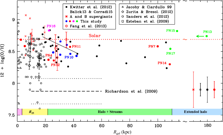
Figure 19.— Radial distribution of oxygen in M31. Galactocentric distances ($R_{\rm gal}$) have been corrected for the inclination of M31 disk. Our GTC sample are the color-filled circles, color-coded in the same manner as in previous figures. Note that the radial distance of PN13 ($\sim$180 kpc) is estimated assuming that it is on the extended disk, and is only an upper limit. Other data sets (see the legend) are explained in the text. The solid black line is a linear fit to the outer-disk PNe of Kwitter et al. (2012, 18$\lesssim$$R_{\rm gal}\lesssim$43 kpc). Typical error bars of different samples are given in the bottom-right corner. The horizontal red-dotted line marks the solar value (8.69, Asplund et al., 2009). In order for convenience in abundance comparison, the distance between 115 and 170 kpc is not properly scaled. The horizontal black-dashed and dotted lines represent the mean metallicity and dispersion of halo stars between 10 and 60 kpc (estimated from the measurements of Richardson et al. 2009). The colored bars in the figure bottom mark the radii of M31’s bulge (pink; $\sim$3.4 kpc, Irwin et al., 2005), the optical disk (yellow; $R_{25}\approx$22 kpc), and the outer halo as well as the farthest outreach of the Giant Stream (green; $\sim$8$\arcdeg$, corresponding to 110 kpc in projection); further out is more extended halo (light blue).

The radial distribution of oxygen in M31 represented by our PNe is shown in Figure 19, where literature samples are also presented, including the M31 disk and bulge PNe from Jacoby & Ciardullo (1999) and Sanders et al. (2012), the outer-disk PNe from Kwitter et al. (2012), Balick et al. (2013) and Corradi et al. (2015), M31 H ii regions from Esteban et al. (2009, object ID K932) and Zurita & Bresolin (2012, nine objects with $T_{\rm e}$ determined), and three A-F supergiants from Venn et al. (2000) and seven B-type supergiants from Trundle et al. (2002). Galactocentric distances ($R_{\rm gal}$) have been rectified for the inclination of M31 disk (see caption of Figure 1).

In Figure 19 we mark the radii of M31’s bulge, the inner/optical disk ($R_{25}$, see caption), the halo (as well as the boundary of streams), and the extended halo. The bulge radius is adopted from Irwin et al. (2005) and well accommodates the bulge PNe studied by Jacoby & Ciardullo (1999). Almost all the disk PNe observed by Kwitter et al. (2012, also and ) are beyond $R_{25}$. The oxygen abundances of M31 disk PNe seem to show a marginally negative gradient ($-$0.011$\pm$0.004 dex kpc^-1, Kwitter et al., 2012) within 40 kpc from the centre of M31, and tend to flatten out to $\gtrsim$100 kpc. In our halo sample, members of which are mostly associated with the substructures of M31, we also found a similar trend of flattening in oxygen. In Paper II, based on a limited sample, we drew a conclusion that the PNe in the Northern Spur and those associated with the Giant Stream have homogeneous oxygen abundances (see Figure 13 in Paper II). Including the ten new targets (PN8–PN17), our extended sample displays generally consistent oxygen abundances.

A very prominent feature in Figure 19 is the solar oxygen of the outermost nebula PN13. Its apparent galactocentric radius is 42 kpc (Table 1); if we assume that PN13 is in the extended disk of M31 (Ibata et al., 2005), its rectified radius will be $\sim$180 kpc, which could be set as an upper-limit distance of this PN. The 12+$\log$(O/H) value of PN15 is 0.13 dex above the Sun (8.69, Asplund et al., 2009), a difference that is close to the typical uncertainty in oxygen of our sample. However, the exact galactocentric radii of PN13 and PN15 are unknown because of the dubious disk membership according to their kinematics (Figure 2).

Another halo object PN17 has an oxygen abundance $\sim$0.15 dex below the Sun. A galactocentric radius of 109 kpc is estimated for PN17, if we assume that it is in the outer disk. However, considering that its radial velocity deviates significantly from the extended disk (Figure 2, bottom), PN17 is probably a halo PN, or even associated with its substructure. PN17 is located near the NE Shelf, an overdensity of metal-rich RGB, whose stellar populations were found to be similar to those of the Giant Stream (Ferguson et al., 2005). Numerical simulations have suggested that the NE Shelf might be debris from the continuation of the Giant Stream (Ibata et al., 2004; Fardal et al., 2008; Mori & Rich, 2008). Given that the oxygen abundance of PN17 is very close to that of PN7, which is well associated with the Giant Stream (Fang et al., 2015), we thus suggest that PN17 might be associated with the NE Shelf.

PN14 is located in the southeast outer halo of M31, and has a rectified galactocentric distance of 108 kpc if we assume that it is in the extended disk. Its oxygen abundance is $\sim$0.4 dex below the Sun. According to its radial velocity and location, we suggest that PN14 might be associated with the Giant Stream (while in Merrett et al. 2006 this PN was not identified to be related to any substructure). Although compared to PN7, PN14 is not located right on the stellar orbit proposed by Merrett et al. (2003, see also Figure 2), considering the large spatial extension (along the direction orthogonal to the stream) of the Giant Stream (McConnachie et al., 2003), this association is possible. As reported in Section 3.6, PN14 has been observed by Corradi et al. (2015, PN ID M2507), who used the same instrument. The difference in 12+$\log$(O/H) between the two observations is well within the measurement uncertainty; the galactocentric distance of PN14 given by Corradi et al. (2015, 106 kpc) is slightly smaller than ours, which is due to a slightly different distance to M31 adopted. If we assume PN14 belongs to the Giant Stream, by applying its three-dimensional structure (McConnachie et al., 2003), we estimate a distance of roughly 50 kpc for this PN. The galactocentric distances of PN14 and PN17 are both uncertain.

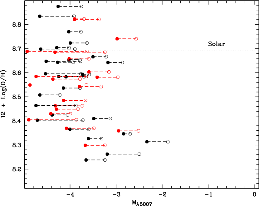
Figure 20.— Oxygen abundances of M31 PNe versus the absolute magnitudes at [O iii] $\lambda$5007. Our halo/substructure PNe are red symbols, and the outer-disk PNe are black. For each PN, the [O iii] magnitudes with and without extinction correction (filled and open circles, respectively) are both presented and connected by a dash line. Solar oxygen is marked by a horizontal dotted line.

Although PN8, PN9 and PN10 have been identified by Merrett et al. (2006) as in the Northern Spur (Table 1), their oxygen abundances are different: the former two PNe are both close to the Sun, while the latter is 0.23 dex below the solar value (Figure 19). These three PNe, together with the other six in the Norther Spur, form a sample in this substructure with 12+$\log$(O/H)$\sim-$0.26–0. Being 0.13 dex above the Sun, the 12+$\log$(O/H) value of PN16 is among the highest in our sample. The galactocentric distance of PN16 (22.6 kpc) was estimated using the distances to M31 (785 kpc) and M32 (763 kpc, Karachentsev et al., 2004) and its angular distance ($\sim$0$\fdg$4) to the centre of M31. It is interesting to note that the oxygen abundance of PN16 seems to well fit the trend of the weakly negative gradient represented by the disk PNe of Kwitter et al. (2012).

Together with the M31 outer-disk PNe, our halo targets are metal-rich ([O/H]$\sim-$0.4 to 0) compared to the mean metallicities of the dominant stellar populations at similar galactocentric radii in the outer halo ([Fe/H]$\lesssim-$1.5 to $\sim-$0.6; e.g., Brown et al. 2006a, 2008; Chapman et al. 2006, 2008; Koch et al. 2008; Richardson et al. 2009). In contrast with the high degree of inhomogeneity in the metallicity of M31’s extended halo (from the most metal-poor population in the outer regions with $-2.5<$[Fe/H]$<-1.7$, to the relatively metal-rich population in the inner halo where $-0.6<$[Fe/H]$\lesssim$0; Ibata et al. 2014), the averaged values of [O/H] of our halo PNe in different kinematic groups (i.e., different substructures) are quite similar, $\sim-0.2$ to 0, with modest dispersion, and are consistently higher than the average [Fe/H] of stars in the respective substructures. The uniformly high oxygen abundances of our PNe indicate that they formed from metal-rich ISM, and probably belong to the population that is distinct from the underlying halo populations of M31.

All PNe selected for our spectroscopic observations are among the brightest in M31, within 2 magnitudes from the bright cut-off of the [O iii] PNLF, which allows a reliable spectral analysis and accurate abundance determinations (Section 3). Whether the metallicity of bright PNe depends on the [O iii] luminosity still needs careful studies, although this possible relation has previously been investigated for the PNe in LMC (Richer, 1993), M31 (Jacoby & Ciardullo, 1999), M32 (Richer & McCall, 2008), M33 and the Milky Way (e.g., Magrini et al., 2004). In these galaxies, oxygen abundances of the bright PNe are found to be independent of the [O iii] absolute magnitude ($M_{\lambda 5007}$), and the brightest PNe are representative of the whole PN population. For the bright PNe ($M_{\lambda 5007}\leq-$3.7) in M31’s outer disk, oxygen abundance has no dependence on $M_{\lambda 5007}$, although a slight tendency of decreasing oxygen seems to exist in a few objects on the fainter tail (Corradi et al., 2015, Figure 4 therein). A very similar trend was found in our halo/substructure sample (Figure 20). Here $M_{\lambda 5007}$ were derived from the [O iii] apparent magnitudes ($m_{\lambda 5007}$, adopted from Merrett et al. 2006), which were corrected for the foreground (and also internal) extinction using $c$(H$\beta$).

Moreover, as predicted by the new post-AGB evolutionary models, low-mass central stars of PNe evolve much faster than previously thought (Miller Bertolami, 2016; Gesicki et al., 2017), thus increasing the possibility that lower mass (and thus relatively older) stars may also form bright PNe that are still visible. Our population analysis (Section 4.2; Table 9) also indicates that bright PNe might evolve from low-mass stars, which is different from the traditional view that bright PNe evolve from rare, high-mass progenitors (e.g., Schönberner et al., 2007). Hence, we conclude that our sample well represents the population of PNe in the halo of M31, regardless of their spatial locations and kinematics. As one of the most efficient coolants in PNe, the [O iii] $\lambda$5007 luminosity is highly dependent on the central star effective temperature (Dopita et al., 1992; Schönberner et al., 2007), but is also regulated by the nebular metallicity (in particular, the fraction of oxygen in O²⁺); thus slight dependency of the [O iii] $\lambda$5007 luminosity on oxygen abundance may exist.

The discussion above is based on the assumption that oxygen is neither created nor destroyed during the evolution of PN progenitors (in our case, low-mass stars; Section 4.2), although third dredge-up and HBB might enhance the oxygen of some AGB stars (e.g., Karakas & Lattanzio, 2014; Delgado-Inglada et al., 2015). In order to compare with M31’s halo metallicities indicated by [Fe/H], we also assumed that [Fe/O]$\approx$0 (i.e., the solar case) for the bright PNe in M31.

4.5. Possible origin of Luminous PNe
in the Halo of M31

Our previous studies of the M31 halo PNe associated with substructures were based on two a priori assumptions: 1) these PNe represent the stellar populations of the substructures where they are located (i.e., they formed in situ); and 2) the PNe associated with substructures have different origins – and thus probably belong to different populations – from those in the disk of M31. However, so far we did not find any discernible difference between our halo sample and the outer-disk PNe in the radial distribution of oxygen at $R_{\rm gal}\lesssim$110 kpc (Figure 19).

Based on the old post-AGB evolutionary models, as were adopted by Kwitter et al. (2012), the stellar ages of our halo sample and the outer-disk sample are both constrained to be $\lesssim$2–3 Gyr. These M31 PNe thus are the young population, with their stellar ages in line with the episode of star formation that occurred across the whole disk system of M31 2–4 Gyr ago (e.g., Richardson et al., 2008; Bernard et al., 2012, 2015a, 2015b; Williams et al., 2015). The onset of this recent global starburst may correspond to an encounter with M33, whose stellar disk also experienced enhanced star formation $\sim$2 Gyr ago (Williams et al., 2009; Bernard et al., 2012). This M31-M33 interaction also explains the stellar streams seen in the M31 halo (McConnachie et al., 2009), and has been invoked to account for the luminous, oxygen-rich PNe in M31’s outer disk (Balick et al., 2013; Corradi et al., 2015).

However, using the well assessed new post-AGB evolutionary models, we confined the main-sequence ages of our halo sample to be mostly $\sim$2–5 Gyr, with the oldest being $\sim$6–8 Gyr; while the outer-disk sample are mostly $\lesssim$1–4 Gyr. We thus conjecture that our targets probably formed prior to the encounter with M33. Obviously, our sample represents the population that is different from the underlying, smooth, extended (and mostly metal-poor) halo component of M31 (Ibata et al., 2007, 2014), which was formed through repeated accretion of smaller galaxies in the distant past. These bright PNe seem to resemble the younger, metal-rich population in the outer stream of M31, as revealed by HST pencil-beam pointings on the Giant Stream (Brown et al., 2006a; Bernard et al., 2015a). The metallicity of the stream fields enriched continuously from [Fe/H]$\sim-$1.5, to at least solar level about 5 Gyr ago (Bernard et al., 2015a). This timeline of metal enrichment is generally consistent with the stellar ages of our metal-rich sample. $N$-body simulations suggested that the Giant Stream and other stream-like features in the halo are debris of a massive ($\gtrsim$10⁹–10${}^{10}\,M_{\sun}$) progenitor that was recently disrupted during the course of merger (e.g., Ibata et al., 2004; Geehan et al., 2006; Font et al., 2006; Fardal et al., 2006, 2007, 2008, 2013; Mori & Rich, 2008; Sadoun et al., 2014). The extended star-formation history and a broad range of metallicity ($-$1.5$\lesssim$[Fe/H]$\lesssim$0.2) discovered in the stream fields can be explained by a disk galaxy progenitor (Brown et al., 2006a, b; Bernard et al., 2015a). If the stellar streams in M31’s halo indeed have a common origin, our sample of halo PNe then probably formed through extended star formation in this possibly massive, disk-like progenitor. Moreover, some simulations predict that the remnant of the disrupted satellite resides in the NE Shelf (e.g., Fardal et al., 2008, 2013; Sadoun et al., 2014); PN17 in our sample is located in this region and might be associated with this substructure (see Section 4.4).

On the other hand, despite the systematic discordance in the estimated stellar ages (and also in kinematics) between the two samples of M31 PNe, their consistently high oxygen abundances (see Figure 19) signifies something maybe in common. Recently, it was suggested that the PNe associated with the outer stellar streams might have formed from the same metal-rich ISM as did the outer-disk sample, but acquired the kinematics of the streams during a subsequent encounter with M33 (Balick et al., 2017). This postulation hints at a possibility that the halo PNe on the streams might have their origins in the M31 disk, where the metal-rich ISM mostly resides. The close interaction between M31 and M33, combined with the recent impact of the Giant Stream’s progenitor, could heat up the main disk and redistribute the disk material into the substructures we see today (Bernard et al., 2015a).

The interpretations presented above are highly speculative, given that the M31 halo is extremely complex and the samples of PNe with high-quality spectroscopic observations are still very limited. In addition, Magrini et al. (2016) suggested that radial migration of the inner-disk PNe in M31 could be important and explain the flattening of oxygen gradient (compared to the H ii regions). This migration mechanism unlikely occurred to our halo PNe because to fling a star inside the disk into halo regions far beyond $R_{25}$ requires many orbital scatterings due to gravitational anomalies, such as dense spiral arms (e.g, Binney & Tremaine, 2008).

A recent proper motion analysis and cosmological simulations of the M31-M33 system suggests it is unlikely that M33 made a recent ($<$3 Gyr), close ($<$100 kpc) passage about M31 (Patel et al., 2017); this is inconsistent with the scenario proposed by McConnachie et al. (2009, also ). If true, the interactions between M31 and the Giant Stream’s progenitor then seem more plausible to explain the kinematics of the metal-rich PNe in the M31 halo.

M32 was speculated to be responsible for the Giant Stream (Ibata et al., 2001a; Ferguson et al., 2002; Choi et al., 2002; Merrett et al., 2003), but kinematical studies ruled out this possibility (Ibata et al., 2004). The stellar orbit proposed by (Merrett et al. 2003; see Figure 2) that links the Giant Stream to the Northern Spur is rather generic yet highly schematic. The light-of-sight distance to M32, although previously derived (e.g., Jensen et al., 2003; Karachentsev et al., 2004), is still uncertain. The N/O ratio of PN16 is higher than our halo PNe, also casting doubts on the previous hypothesis that M32 was the progenitor of substructures.

4.6. Comments on Individual Objects

Several PNe in our GTC sample are interesting in terms of abundances, spatial locations, and kinematics, and worth extra attention. Although most of these PNe have already been discussed in previous sections, their main characteristics are briefly emphasized here.

PN7 — The mostly distant PN so far studied in the extended halo of M31. Well located in the southeast extension of the Giant Stream and with an oxygen abundance close to the Sun, PN7 is an archetypal object that represents the group of metal-rich nebulae associated with the outer-halo streams at large galactocentric radii.

PN13 — An outer-halo PN spatially located on the Giant Stream. If we assume that PN13 is in the extended disk, its rectified galactocentric distance will be $\sim$180 kpc, making it the most distant solar-metallicity PN in M31 so far observed. However, its disk membership is highly questionable due to kinematics.

PN14 — It might be associated with the Giant Stream. Its oxygen is $\sim$0.4 dex below the Sun, but is close to those of PN4 and PN12 on the stream.

PN15 — Its oxygen is $\sim$0.13 dex above the Sun, making it the most metal-rich PN so far observed in the outer halo of M31. Same as PN13, its actual distance to the centre of M31 is unclear.

PN16 — The only M32 PN analyzed in this work. Its O/H and N/O ratios are both higher than the other PNe in our sample. PN16 also has the highest oxygen abundance among all PNe so far spectroscopically studied in M32 (Richer et al., 1999). The estimated stellar age ($t_{\rm ms}\sim$2 Gyr) of PN16 is consistent with the younger stellar population discovered in M32 (2–5 Gyr, Monachesi et al., 2012). This bright PN ($m_{\lambda 5007}$=20.78) probably well represents the young population of M32. Given that currently reliable abundance measurements of the M32 PNe are extremely sparse, our observations provide valuable nebular abundances of this dwarf elliptical galaxy.

PN17 — This halo PN might be associated with the NE Shelf, as judged from its O/H, spatial position, and kinematics (see the discussion in Section 4.4). If it is true, PN17 will be the first PN discovered and studied in this halo substructure.

5. Summary, Conclusion
and Future Work

With the aim of studying the properties and possible origins of stellar substructures in the halo of M31, we carry out deep spectroscopy of PNe using the 10.4 m GTC. Following our previous effort (Fang et al., 2015), where seven PNe associated with the Northern Spur and the Giant Stream were targeted, we obtained high-quality GTC long-slit spectra of ten PNe that reside at different regions and cover a vast area of the M31 system. These new targets are associated with the two known substructures, the eastern and southern regions of M31’s halo, and dwarf satellite M32. The OSIRIS spectrograph secures a wavelength coverage of $\sim$3630–7850 Å and detection of a number of plasma-diagnostic emission lines, including the temperature-sensitive [O iii] $\lambda$4363 and [S iii] $\lambda$6312 lines and the density-diagnostic [S ii] $\lambda\lambda$6716,6731 doublet. We also observed the [S iii] $\lambda\lambda$9069,9531 nebular lines in four PNe, whose GTC spectrum extends beyond 1 $\mu$m. Ionic and elemental abundances (relative to hydrogen) of helium, oxygen, nitrogen, neon, sulfur, argon and chlorine were derived using different temperatures and densities according to ionization stages.

The N/O ratios of our halo sample are mostly $<$0.4, and He/H$<$0.126, indicating that they might be Type II, i.e., of relatively low-mass progenitors. These abundance are generally consistent with the outer-disk sample recently observed with the 8–10 m telescopes (Kwitter et al., 2012; Balick et al., 2013; Corradi et al., 2015). In both samples, Ne/H is well correlated with O/H; in some objects, argon is under-abundant with respect to the Ar/H versus O/H correlation. The “sulfur anomaly”, originally found in Galactic PNe, also exists in the M31 PNe, even for the objects with detection of the [S iii] $\lambda\lambda$9069,9531 lines. Although with large scatter, Cl/H of our targets are generally in line with the Cl/H versus O/H correlation as defined by the Galactic H ii regions with best measurements of chlorine. In an M32 PN, we found a relatively high N/O ratio ($\sim$1.07$\pm$0.24).

The central star temperatures and luminosities of our targets were derived using the empirical method. In the H-R diagram, our sample occupies the regions that correspond to relatively lower core masses than does the outer-disk sample. As constrained using the new post-AGB evolutionary models, which have recently been assessed through studies of Galactic PNe, the core masses of our sample of halo PNe are 0.53–0.58 $M_{\sun}$, and those of the outer-disk sample are 0.55–0.64 $M_{\sun}$; the main-sequence ages of our targets are then mostly $\sim$2–5 Gyr, with the oldest being $\sim$6–8 Gyr; while the outer-disk PNe are mostly $\sim$1–4 Gyr. If the new post-AGB evolutionary models are adopted in our population analysis, the PNe so far observed in M31 probably all evolved from low-mass ($\lesssim$2.2 $M_{\sun}$) progenitors, which formed from the metal-rich ([O/H]$\gtrsim-$0.4) ISM. In the H-R diagram, our GTC targets are mostly located before the theoretical isochrone of 10 000 yr since the beginning of post-AGB evolution; given that they are the brightest PNe in M31, their locations in the diagram are generally consistent with the high probability that these nebulae are not quite evolved in the PN phase and still stay around their peak [O iii] luminosities. Our estimated central star parameters thus are, although still preliminary, generally reasonable and suggest that the brightest PNe in M31 are probably optically thick.

The He/H, O/H, N/O and Ne/H ratios of both samples of M31 PNe were compared with the AGB nucleosynthesis models, and general consistency between the observations and theoretical predictions of AGB yields was found. From the model-predicted abundance ratios, we constrained the upper-limits of the initial stellar masses of both samples of M31 PNe to be $<$3 $M_{\sun}$, in line with our mass estimate based on the new post-AGB evolutionary models. We also studied the dependence of abundance ratios on initial mass, and found in overall excellent agreement. In particular, as a stellar-mass indicator, the observed N/O ratios mostly agree, within the errors, with the AGB models of Karakas et al. at low masses (1–3 $M_{\sun}$), except for several outliers. Although still limited by the sample size, N/O of M31 PNe seems to start to increase at $\lesssim$2 $M_{\sun}$, a trend similar to what has been recently found in Galactic PNe, indicating that HHB might actually occur in very low-mass stars. According to the AGB models, O/H of the combined sample of M31 PNe span a broad range that encompasses the metallicities of the SMC ($Z$=0.004) and the Sun ($Z\lesssim$0.02), irrespective of the initial masses. The O/H ratios of our halo sample are similar to those of the outer-disk PNe. From the oxygen abundance, spatial location and kinematics, we suggest that PN17 in the eastern halo might belong to the NE Shelf.

Our extended sample of the halo/substructure PNe exhibit uniformly high oxygen abundances with modest scatter. We found nearly-solar oxygen in several PNe that are located in the outer halo. The most interesting target with solar oxygen is on the southeast extension of the Giant Stream, with a sky-projected galactocentric distance of $\sim$50 kpc. In one of the outermost PNe, we even found slightly over-solar oxygen ([O/H]$\approx$0.13); there is also a halo target in our GTC sample with slightly sub-solar oxygen, [O/H]$\sim-$0.4. Our targets probably belong to the population that is different from the underlying, smooth halo component of M31, but more like the metal-rich populations in the streams. The estimated stellar ages of our sample (mostly $\sim$2–5 Gyr) are consistent with the metal enrichment history recently unveiled in the stellar fields of the Giant Stream. If the substructures where our targets are associated have a common origin (i.e., they are tidal debris from a possibly massive, disk-like satellite of M31), our deep spectroscopy of nebulae confirms the extended star-formation history in this satellite that was previously unveiled through HST photometric studies. Alternatively, our observations cannot exclude the possibility that our targets might originally formed in the M31 disk, but were scattered to the halo regions and gained their current stream kinematics as a result of interactions with M31’s satellite, which can heat up and perturb the stellar disk and redistribute the disk material. Either of the above two interpretations supports the current astrophysical picture that M31’s halo evolved through complex galactic mergers and interactions.

Through unprecedentedly deep spectroscopy of a sample of PNe mostly associated with the substructures in the halo of M31, we have obtained intriguing results which, together with the recent spectroscopic observations of the outer-disk sample by other research groups at the 8–10 m class telescopes, may have profound effects in our understanding of the M31 system, especially its highly structured extended halo, which so far has been rarely investigated through quantitative spectroscopy of the ISM. Our findings are qualitatively consistent with the complexity of M31’s giant halo. However, one still needs to realize that at this stage no definite conclusions can be drawn and all interpretations are highly speculative, given the limited PN samples and the complex evolutionary history of M31.

The number of PNe discovered and identified in the outskirts of M31 has been increased in recently years. To date our observations mainly focus on the PNe in the Northern Spur and the Giant Stream substructures that cover the southeast, the eastern and the northern regions of the halo. In the follow-up observations at the 10 m GTC, we target the western halo objects and extend further north and south, $>$2$\arcdeg$ from the centre of M31. Through these combined efforts, we aim to construct a statistically significant and spatially unbiased sample for detailed analysis (including photoionization modeling), to make a census study of M31’s extended halo, and eventually to obtain a grand picture of its evolution.

References

- Acker & Neiner (2003) Acker, A., & Neiner, C. 2003, A&A, 403, 659
- Asplund et al. (2009) Asplund, M., Grevesse, N., Sauval, A.-J., & Scott, P. 2009, ARA&A, 47, 481
- Balick et al. (2013) Balick, B., Kwitter, K. B., Corradi, R. L. M., & Henry, R. B. C. 2013, ApJ, 774, 3
- Balick et al. (2017) Balick, B., Kwitter, K. B., Corradi, R. L. M., Galera Rosillo, R., & Henry, R. B. C. 2017, in IAU Symp. 323, Planetary Nebulae: Multi-wavelength Probes of Stellar and Galactic Evolution, ed. X.-W. Liu, L. Stanghellini & A. I. Karakas (Cambridge: Cambridge Univ. Press), 264
- Bell et al. (1995) Bell, K. L., Hibbert, A., & Stafford, R. P. 1995, PhyS, 52, 240
- Bernard et al. (2012) Bernard, E. J., Ferguson, A. M. N., Barker, M. K., et al. 2012, MNRAS, 420, 2625
- Bernard et al. (2015b) Bernard, E. J., Ferguson, A. M. N., Chapman, S. C., et al. 2015b, MNRAS, 453, L113
- Bernard et al. (2015a) Bernard, E. J., Ferguson, A. M. N., Richardson, J. C., et al. 2015a, MNRAS, 446, 2789
- Biémont & Hansen (1986) Biémont, E., & Hansen, J. E. 1986, PhyS, 34, 116
- Binney & Tremaine (2008) Binney, J., & Tremaine, S. 2008, Galactic Dynamics (2nd ed.; Princeton, NJ: Princeton Univ. Press)
- Blöcker (1995) Blöcker, T. 1995, A&A, 299, 755
- Brown et al. (2008) Brown, T. M., Beaton, R., Chiba, M., et al. 2008, ApJ, 685, L121
- Brown et al. (2006a) Brown, T. M., Smith, E., Ferguson, H. C., et al. 2006a, ApJ, 652, 323
- Brown et al. (2006b) Brown, T. M., Smith, E., Guhathakurta, P., et al. 2006b, ApJ, 636, L89
- Caldwell et al. (2010) Caldwell, N., Morrison, H., Kenyon, S. J., et al. 2010, AJ, 139, 372
- Cantiello & Langer (2010) Cantiello, M., & Langer, N. 2010, A&A, 521, A9
- Cardelli et al. (1989) Cardelli, J. A., Clayton, G. C., & Mathis, J. S. 1989, ApJ, 345, 245
- Carignan et al. (2006) Carignan, C., Chemin, L., Huchtmeier, W. K., & Lockman, F. J. 2006, ApJ, 641, L109
- Catalán et al. (2008) Catalán, S., Isern, J., García-Berro, E., & Ribas, I. 2008, MNRAS, 387, 1693
- Chapman et al. (2008) Chapman, S.C., Ibata, R. A., Irwin, M., et al. 2008, MNRAS, 390, 1437
- Chapman et al. (2006) Chapman, S.C., Ibata, R. A., Lewis, G. F., et al. 2006, ApJ, 653, 255
- Charbonnel & Lagarde (2010) Charbonnel, C., & Lagarde, N. 2010, A&A, 522, A10
- Choi et al. (2002) Choi, P. I., Guhathakurta, P., & Johnson, K. V. 2002, AJ, 124, 310
- Ciardullo (2010) Ciardullo, R. 2010, PASA, 27, 149
- Ciardullo et al. (1989) Ciardullo, R., Jacoby, G. H., Ford, H. C., & Neill, J. D. 1989, ApJ, 339, 53
- Clayton (2003) Clayton, D. D. 2003, in Handbook of Isotopes in the Cosmos, (Cambridge: Cambridge University Press), 163
- Corbelli et al. (2010) Corbelli, E., Lorenzoni, S., Walterbos, R., Braun, R., & Thilker, D. 2010, A&A, 511, A89
- Corradi et al. (2015) Corradi, R. L. M., Kwitter, K. B., Balick, B., Henry, R. B. C., & Hensley, K. 2015, ApJ, 807, 181
- Cristallo et al. (2011) Cristallo, S., Piersanti, L., Straniero, O., Gallino, R., Domínguez, I., Abia, C., Di Rico, G., Quintini, M., & Bisterzo, S. 2011, ApJS, 197, 17
- Cristallo et al. (2015) Cristallo, S., Straniero, O., Piersanti, L., & Gobrecht, D. 2015, ApJS, 219, 40
- Crowther et al. (1998) Crowther, P. A., De Marco, O., & Barlow, M. J. 1998, MNRAS, 296, 367
- Cui et al. (2004) Cui, X.-Q., Su, D.-Q., Li, G.-P., et al. 2004, Proc. SPIE, 5489, 974
- Cui et al. (2010) Cui, X.-Q., Su, D.-Q., Wang, Y.-N., et al. 2010, Proc. SPIE, 7733, 7
- Cui et al. (2012) Cui, X.-Q., Zhao, Y.-H., Chu, Y.-Q., et al. 2012, RAA, 12, 1197
- Davey et al. (2000) Davey, A. R., Storey, P. J., & Kisielius, R. 2000, A&AS, 142, 85
- de Vaucouleurs (1958) de Vaucouleurs, G. 1958, ApJ, 128, 465
- de Vaucouleurs et al. (1991) de Vaucouleurs, G., de Vaucouleurs, A., Corwin, H. G., Jr., et al. 1991, Third Reference Catalogue of Bright Galaxies (New York: Springer)
- Delgado-Inglada et al. (2014) Delgado-Inglada, G., Morisset, C., & Stasińska, G. 2014, MNRAS, 440, 536
- Delgado-Inglada et al. (2015) Delgado-Inglada, G., Rodríguez, M., Peimbert, M., Stasińska, G., & Morisset, C. 2015, MNRAS, 449, 1797
- Di Criscienzo et al. (2016) Di Criscienzo, M., Ventura, P., García-Hernández, D. A., et al. 2016, MNRAS, 462, 395
- Dopita et al. (1992) Dopita, M. A., Jacoby, G. H., & Vassiliadis, E. 1992, ApJ, 389, 27
- Dopita & Meatheringham (1990) Dopita, M. A., & Meatheringham, S. J. 1990, ApJ, 357, 140
- Dopita & Meatheringham (1991) Dopita, M. A., & Meatheringham, S. J. 1991, ApJ, 377, 480
- Dufour et al. (2015) Dufour, R. J., Kwitter, K. B., Shaw, R. A., Henry, R. B. C., Balick, B., & Corradi, R. L. M. 2015, ApJ, 803, 23
- Esteban et al. (2009) Esteban, C., Bresolin, F., Peimbert, M., et al. 2009, ApJ700, 654
- Esteban et al. (2015) Esteban, C., García-Rojas, J., & Pérez-Mesa, V. 2015, MNRAS, 452, 1553
- Esteban et al. (2004) Esteban, C., Peimbert, M., García-Rojas, J., et al. 2004, MNRAS, 355, 229
- Fang et al. (2015) Fang, X., García-Benito, R., Guerrero, M. A., Liu, X.-W., Yuan, H.-B., Zhang, Y., & Zhang, B. 2015, ApJ, 815, 69 (Paper II)
- Fang & Liu (2013) Fang, X., & Liu, X.-W. 2013, MNRAS, 429, 2791
- Fang et al. (2013) Fang, X., Zhang, Y., García-Benito, R., Liu, X.-W., & Yuan, H.-B. 2013, ApJ, 774, 138 (Paper I)
- Fardal et al. (2006) Fardal, M. A., Babul, A., Geehan, J. J., & Guhathakurta, P. 2006, MNRAS, 366, 1012
- Fardal et al. (2008) Fardal, M. A., Babul, A., Guhathakurta, P., Gilbert, K. M., & Dodge, C. 2008, ApJ, 682, L33
- Fardal et al. (2007) Fardal, M. A., Guhathakurta, P., Babul, A., & McConnachie, A. W. 2007, MNRAS, 380, 15
- Fardal et al. (2013) Fardal, M. A., Weinberg, M. D., Babul, A., et al. 2013, MNRAS, 434, 2997
- Ferguson et al. (2002) Ferguson, A. M. N., Irwin, M. J., Ibata, I. A., Lewis, G. F., & Tanvir, N. R. 2002, AJ, 124, 1452
- Ferguson et al. (2005) Ferguson, A. M. N., Johnson, R. A., Faria, D. C., et al. 2005, ApJ, 622, L109
- Ferland et al. (2013) Ferland, G. J., Porter, R. L., van Hoof, P. A. M., et al. 2013, RMxAA, 49, 137
- Fishlock et al. (2014) Fishlock, C. K., Karakas, A. I., Lugaro, M., & Yong, D. 2014, ApJ, 797, 44
- Font et al. (2006) Font, A. S., Johnston, K. V., Guhathakurta, P., Majewski, S. R., & Rich, R. M. 2006, AJ, 131, 1436
- Frew et al. (2016) Frew, D. J., Parker, Q. A., & Bojičić, I. S. 2016, MNRAS, 455, 1459
- Galavis et al. (1995) Galavis, M. E., Mendoza, C., & Zeippen, C. J. 1995, A&AS, 111, 347
- García-Rojas et al. (2016) García-Rojas, J., Peña, M., Flores-Durán, S., & Hernández-Martínez, L. 2016, A&A, 586, A59
- Geehan et al. (2006) Geehan, J. J., Fardal, M. A., Babul, A., & Guhathakurta, P. 2006, MNRAS, 366, 996
- Gerhard et al. (2005) Gerhard, O., Arnaboldi, M., Freeman, K. C., Kashikawa, N., Okamura, S., & Yasuda, N. 2005, ApJ, 621, L93
- Gerhard et al. (2007) Gerhard, O., Arnaboldi, M., Freeman, K. C., Okamura, S., Kashikawa, N., & Yasuda, N. 2007, A&A, 468, 815
- Gesicki et al. (2014) Gesicki, K., Zijlstra, A. A., Hajduk, M., & Szyszka, C. 2014, A&A, 566, A48
- Gesicki et al. (2017) Gesicki, K., Zijlstra, A. A., Miller Bertolami, M. M. 2017, in ASP Conf. Ser. 509, 20th European White Dwarf Workshop, ed. P.-E. Tremblay, B. Gänsicke, & T. Marsh (San Francisco: ASP), 457
- Grevesse & Noels (1993) Grevesse, N., & Noels, A. 1993, In Origin of Evolution of the Elements, ed. N. Prantzos et al. (Cambridge: Cambridge University Press), 15
- Grevesse & Sauval (1998) Grevesse, N., & Sauval, A. J. 1998, Space Sci. Rev., 85, 161
- Henry (1989) Henry, R. B. C. 1989, MNRAS, 241, 453
- Henry et al. (2004) Henry, R. B. C., Kwitter, K. B., & Balick, B. 2004, AJ, 127, 2284
- Henry et al. (2010) Henry, R. B. C., Kwitter, K. B., Jaskot. A. E., Balick, B., Morrison, M. A., & Milingo, J. B. 2010, ApJ, 724, 748
- Henry et al. (2012) Henry, R. B. C., Speck, A., Karakas, A. I., Ferland, G. J., & Maguire, M. 2012, ApJ, 749, 61
- Henry et al. (2018) Henry, R. B. C., Stephenson, B. G., Miller Bertolami, M. M., Kwitter, K. B., & Balick, B. 2018, MNRAS, 473, 241
- Herwig (2005) Herwig, F. 2005, ARA&A, 43, 435
- Hirata & Horaguchi (1994) Hirata, R., & Horaguchi, T. 1994, yCat, 6069, 0
- Howarth & Adams (1981) Howarth, I. D., & Adams, S. 1981, Program EQUIB, Univ. Coll. London, London
- Huchra et al. (1991) Huchra, J. P., Brodie, J. P., & Kent, S. M. 1991, ApJ, 370, 495
- Hurley-Keller et al. (2004) Hurley-Keller, D., Morrison, H. L., & Harding, P. 2004, ApJ, 616, 804
- Ibata et al. (2004) Ibata, R. A., Chapman, S., Ferguson, A. M. N., Irwin, M., Lewis, G., & McConnachie, A. 2004, MNRAS, 351, 117
- Ibata et al. (2005) Ibata, R. A., Chapman, S., Ferguson, A. M. N., Lewis, G., Irwin, M., & Tanvir, N. 2005, ApJ, 634, 287
- Ibata et al. (2001a) Ibata, R. A., Irwin, M. J., Lewis, G. F., Ferguson, A. M. N., & Tanvir, N. R. 2001a, Natur, 412, 49
- Ibata et al. (2001b) Ibata, R. A., Irwin, M. J., Lewis, G. F., & Stotle, A. 2001b, ApJ, 547, L133
- Ibata et al. (2001c) Ibata, R. A., Lewis, G. F., Irwin, M. J., Totten, E., & Quinn, T. 2001c, ApJ, 551, 294
- Ibata et al. (2014) Ibata, R. A., Lewis, G. F., McConnachie, A. W., et al. 2014, ApJ, 780, 128
- Ibata et al. (2007) Ibata, R. A., Martin, N. F., Irwin, M. J., et al. 2007, ApJ, 671, 1591
- Izotov & Thuan (1999) Izotov, Y. I., & Thuan, T. X. 1999, ApJ, 511, 639
- Izotov et al. (2012) Izotov, Y. I., Thuan, T. X., & Guseva, N. G. 2012, A&A, 546, A122
- Irwin et al. (2005) Irwin, M. J., Ferguson, A. M. N., Ibata, R. A., Lewis, G. F., & Tanvir, N. R. 2005, ApJ, 628, L105
- Jacoby (1989) Jacoby, G. H. 1989, ApJ, 339, 39
- Jacoby & Ciardullo (1999) Jacoby, G. H., & Ciardullo, R. 1999, ApJ, 515, 169
- Jensen et al. (2003) Jensen, J. B., Tonry, J. L., Barris, B. J., et al. 2003, ApJ, 583, 712
- Kaler (1986) Kaler, J. B. 1986, ApJ, 308, 322
- Karachentsev et al. (2004) Karachentsev, I. D., Karachentseva, V. E., Huchtmeier, W. K., & Makarov, D. I. 2004, AJ, 127, 2031
- Karakas (2010) Karakas, A. I. 2010, MNRAS, 403, 1413
- Karakas & Lattanzio (2014) Karakas, A. I., & Lattanzio, J. C. 2014, PASA, 31, 30
- Karakas & Lugaro (2016) Karakas, A. I., & Lugaro, M. 2016, ApJ, 825, 26
- Karakas et al. (2014) Karakas, A. I., Marino, A. F., & Nataf, D. M. 2014, ApJ, 784, 32
- Karakas et al. (2009) Karakas, A. I., van Raai, M. A., Lugaro, M., Sterling, N. C., & Dinerstein, H. L. 2009, ApJ, 690, 1130
- Keenan et al. (1993) Keenan, F. P., Hibbert, A., Ojha, P. C., & Conlon, E. S. 1993, PhyS, 48, 129
- Kennicutt et al. (2003) Kennicutt, R. C., Bresolin, F., & Garnett, D. R. 2003, ApJ, 591, 801
- Kingsburgh & Barlow (1994) Kingsburgh, R. L., & Barlow, M. J. 1994, MNRAS, 271, 257
- Kniazev et al. (2014) Kniazev, A. Y., Grebel, E. K., Zucker, D. B., & Rix, H.-W. 2014, AJ, 147, 16
- Koch et al. (2008) Koch, A., Rich, M., Reitzel, D. B., et al. 2008, ApJ, 689, 958
- Kwitter & Henry (2001) Kwitter, K. B., & Henry, R. B. C. 2001, ApJ, 562, 804
- Kwitter et al. (2003) Kwitter, K. B., Henry, R. B. C., & Milingo, J. B. 2003, PASP, 115, 80
- Kwitter et al. (2012) Kwitter, K. B., Lehman, E. M. M., Balick, B., & Henry, R. .B. C. 2012, ApJ, 753, 12
- Landi & Bhatia (2005) Landi, E., & Bhatia, A. K. 2005, ADNDT, 89, 195
- Lennon & Burke (1994) Lennon, D. J., & Burke, V. M. 1994, A&AS, 103, 273
- Liu (2012) Liu, X.-W. 2012, in New Vision 400: Engaging Big Questions in Astronomy and Cosmology Four Hundred Years after the Invention of the Telescope, ed. D. G. York et al. (Boca Raton, FL: CRC Press), 103
- Lodders (2003) Lodders, K. 2003, ApJ, 591, 1220
- Longobardi et al. (2015a) Longobardi, A., Arnaboldi, M., Gerhard, O., & Hanuschik, R. 2015a, A&A, 579, A135
- Longobardi et al. (2015b) Longobardi, A., Arnaboldi, M., Gerhard, O., & Mihos, J. C. 2015b, A&A, 579, L3
- Lugaro et al. (2012) Lugaro, M., Karakas, A. I., Stancliffe, R. J., & Rijs, C. 2012, ApJ, 747, 2
- Maciel (1992) Maciel, W. J. 1992, Ap&SS, 196, 23
- Magrini et al. (2016) Magrini, L., Coccato, L., Stanghellini, L., Casasola, V., & Galli, D. 2016, A&A, 588, A91
- Magrini et al. (2004) Magrini, L., Perinotto, M., Mampaso, A., & Corradi, R. L. M. 2004, A&A, 426, 779
- Manchado et al. (2000) Manchado, A., Villaver, E., Stanghellini, L., & Guerrero, M. A. 2000, in ASP Conf. Ser. 199, Asymmetrical Planetary Nebulae II, ed. J. H. Kastner, N. Soker, & S. Rappaport (San Francisco: ASP), 17
- Majewski et al. (2003) Majewski, S. R., Skrutskie, M. F., Weinberg, M. D., & Ostheimer, J. C. 2003, ApJ, 599, 1082
- Marigo (2001) Marigo, P. 2001, A&A, 370, 194
- McConnachie et al. (2005) McConnachie, A. W., Irwin, M. J., Ferguson, A. M. N., et al. 2005, MNRAS, 356, 979
- McConnachie et al. (2003) McConnachie, A. W., Irwin, M. J., Ibata, R. A., et al. 2003, MNRAS, 343, 1335
- McConnachie et al. (2009) McConnachie, A. W., Irwin, M. J., Ibata, R. A., et al. 2009, Natur, 461, 66
- McConnachie et al. (2004) McConnachie, A. W., Irwin, M. J., Lewis, G. F., et al. 2004, MNRAS, 351, L94
- McLaughlin & Bell (2000) McLaughlin, B. M., & Bell, K. L. 2000, JPhB, 33, 597
- McNabb et al. (2013) McNabb, I. A., Fang, X., Liu, X.-W., Bastin, R. J., & Storey, P. J. 2013, MNRAS, 428, 3443
- Meatheringham & Dopita (1991) Meatheringham, S. J., & Dopita, M. A. 1991, ApJS, 75, 407
- Mendoza (1983) Mendoza, C. 1983, in IAU Symp. 103, Planetary Nebulae, ed. D. Flower (Dordrecht: Reidel), 143
- Mendoza & Zeippen (1982a) Mendoza, C., & Zeippen, C. J. 1982a, MNRAS, 199, 1025
- Mendoza & Zeippen (1982b) Mendoza, C., & Zeippen, C. J. 1982b, MNRAS, 198, 127
- Merrett et al. (2003) Merrett, H. R., Kuijken, K., Merrifield, M. R., et al. 2003, MNRAS, 346, L62
- Merrett et al. (2006) Merrett, H. R., Merrifield, M. R., Douglas, N. G., et al. 2006, MNRAS, 369, 120
- Milingo et al. (2002a) Milingo, J. B., Kwitter, K. B., Henry, R. B. C., & Cohen, R. E. 2002a, ApJS, 138, 279
- Milingo et al. (2002b) Milingo, J. B., Henry, R. B. C., & Kwitter, K. B. 2002b, ApJS, 138, 285
- Milingo et al. (2010) Milingo, J. B., Kwitter, K. B., Henry, R. B. C., & Souza, S. P. 2010, ApJ, 711, 619
- Miller Bertomali (2015) Miller Bertolami, M. M. 2015, in 19th European Workshop on White Dwarfs, ed. P. Dufour, P. Bergeron, & G. Fontaine, ASP Conf. Ser., 493, 83
- Miller Bertolami (2016) Miller Bertolami, M. M. 2016, A&A, 588, A25
- Monachesi et al. (2012) Monachesi, A., Trager, S. C., Lauer, T. R., et al. 2012, ApJ, 745, 97
- Mori & Rich (2008) Mori, M., & Rich, R. M. 2008, ApJ, 674, L77
- Morisset (2016) Morisset, C. 2017, in IAU Symp. 323, Planetary Nebulae: Multi-wavelength Probes of Stellar and Galactic Evolution, ed. X.-W. Liu, L. Stanghellini & A. I. Karakas (Cambridge: Cambridge Univ. Press), 43
- Morisset et al. (2015) Morisset, C., Delgado-Inglada, G., Flores-Fajardo, N. 2015, RMxAA, 51, 101
- Oke (1974) Oke, J. B. 1974, ApJS, 27, 21
- Oke (1990) Oke, J. B. 1990, AJ, 99, 1621
- Osterbrock & Ferland (2006) Osterbrock, D. E., & Ferland, G. J. 2006, Astrophysics of Gaseous Nebulae and Active Galactic Nuclei (Sausalito, CA: Univ. Science Books)
- Patel et al. (2017) Patel, E., Besla, G., & Sohn, S. T. 2017, MNRAS, 464, 3825
- Peimbert (1978) Peimbert, M. 1978, in IAU Symp. 76, Planetary Nebulae, (Dordrecht: D. Reidel Publishing), 215
- Peimbert & Torres-Peimbert (1983) Peimbert, M., & Torres-Peimbert, S. 1983, in IAU Symp. 103, Planetary Nebulae, ed. D. R. Flower (Dordrecht: Reidel), 233
- Pignatari et al. (2016) Pignatari, M., Herwig, F., Hirschi, R., et al. 2016, ApJS, 225, 24
- Porter et al. (2012) Porter, R. L., Ferland, G. J., Storey, P. J., & Detisch, M. J. 2012, MNRAS, 425, L28
- Pottasch (1984) Pottasch, S. R. 1984, Planetary Nebulae (Reidel Dordrecht)
- Pradhan et al. (2006) Pradhan, A. K., Montenegro, M., Nahar, S. N., & Eissner, W. 2006, MNRAS, 366, L6
- Putman et al. (2009) Putman, M. E., Peek, J. E. G., Muratov, A., et al. 2009, ApJ, 703, 1486
- Ramsbottom et al. (1997) Ramsbottom, C. A., Bell, K. L., & Keenan, F. P. 1997, MNRAS, 284, 754
- Ramsbottom et al. (1996) Ramsbottom, C. A., Bell, K. L., & Stafford, R. P. 1996, ADNDT, 63, 57
- Rauch (1997) Rauch, T. 1997, A&A. 320, 237
- Rauch (2003) Rauch, T. 2003, A&A. 403, 709
- Richardson et al. (2008) Richardson, J. C., Ferguson, A. M. N., Johnson, R. A., et al. 2008, ApJ, 135, 1998
- Richardson et al. (2009) Richardson, J. C., Ferguson, A. M. N., Mackey, A. C., et al. 2009, MNRAS, 396, 1842
- Richer (1993) Richer, M. G. 1993, ApJ, 415, 240
- Richer & McCall (2008) Richer, M. G., & McCall, M. L. 2008, ApJ, 684, 1190
- Richer et al. (1999) Richer, M. G., Stasińska, G., & McCall, M. L. 1999, A&AS, 135, 203
- Sadoun et al. (2014) Sadoun, R., Mohayaee, R., & Colin, J. 2014, MNRAS, 442, 160
- Salaris et al. (2009) Salaris, M., Serenelli, A., Weiss, A., & Miller Bertolami, M. M. 2009, ApJ, 692, 1013
- Sanders et al. (2012) Sanders, N. E., Caldwell, N., McDowell, J., & Harding, P. 2012, ApJ, 758, 133
- Savage & Mathis (1979) Savage, B. D., & Mathis, J. S. 1979, ARA&A, 17, 73
- Schaller et al. (1992) Schaller, G., Schaerer, D., Meynet, G., & Maeder, A. 1992, A&AS, 96, 269
- Schönberner (1983) Schönberner, D. 1983, ApJ, 272, 708
- Schönberner et al. (2007) Schönberner, D., Jacob, R., Steffen, M., & Sandin, C. 2007, A&A, 473, 467
- Shaw et al. (2001) Shaw, R. A., Stanghellini, L., Mutchler, M., Balick, B., & Blades, J. C. 2001, ApJ, 548, 727
- Shingles & Karakas (2013) Shingles, L. J., & Karakas, A. I. 2013, MNRAS, 431, 2861
- Shingles et al. (2015) Shingles, L. J., Doherty, C. L., Karakas, A. I., Stancliffe, R. J., Lattanzio, J. C., & Lugaro, M. 2015, MNRAS, 452, 2804
- Stafford et al. (1994) Stafford, R. P., Bell, K. L., Hibbert, A., & Wijesundera, W. P. 1994, MNRAS, 268, 816
- Stanghellini et al. (2006) Stanghellini, L., Guerrero, M. A., Cunha, K., Manchado, A., & Villaver, E. 2006, ApJ, 651, 898
- Stanghellini et al. (2002a) Stanghellini, L., Villaver, E., Manchado, A., & Guerrero, M. A. 2002a, ApJ, 576, 285
- Stanghellini et al. (2002b) Stanghellini, L., Shaw, R. A., Mutchler, M., Palen, S., Balick, B., & Blades, J. C. 2002b, ApJ, 575, 178
- Stanghellini et al. (2003) Stanghellini, L., Shaw, R. A., Balick, B., Mutchler, M., Blades, J. C., & Villaver, E. 2003, ApJ, 596, 997
- Storey & Hummer (1995) Storey, P. J., & Hummer, D. G. 1995, MNRAS, 272, 41
- Storey & Zeippen (2000) Storey, P. J., & Zeippen, C. J. 2000, MNRAS, 312, 813
- Su et al. (1998) Su, D.-Q., Cui, X.-Q., Wang, Y., & Yao, Z. 1998, Proc. SPIE, 3352, 76
- Tanaka et al. (2010) Tanaka, M., Chiba, M., Komiyama, Y., Guhathakurta, P., Kalirai, J., & Iye, M. 2010, ApJ, 708, 1168
- Tayal & Gupta (1999) Tayal, S. S., & Gupta, G. P. 1999, ApJ, 526, 544
- Trundle et al. (2002) Trundle, C., Dufton, P. L., Lennon, D. J., Smartt, S. J., & Urbaneja, M. A. 2002, A&A, 395, 519
- Vassiliadis & Wood (1994) Vassiliadis, E., & Wood, P. R. 1994, ApJS, 92, 125
- Venn et al. (2000) Venn, K. A., McCarthy, J. K., Lennon, D. J., Przybilla, N., Kudritzki, R. P., & Lemke, M. 2000, ApJ, 541, 610
- Ventura et al. (2013) Ventura, P., Di Criscienzo, M., Carini, R., & D’Antona, F. 2013, MNRAS, 431, 3642
- Ventura et al. (2014) Ventura, P., Di Criscienzo, M., D’Antona, F., et al. 2014, MNRAS, 437, 3274
- Ventura et al. (2015) Ventura, P., Karakas, A. I., Dell’Agli, F., et al. 2015, MNRAS, 450, 3181
- Wang & Liu (2007) Wang, W., & Liu, X.-W. 2007, MNRAS, 381, 669
- Wang & Liu (2008) Wang, W., & Liu, X.-W. 2008, MNRAS, 389, L33
- White (1978) White, S. D. M. 1978, MNRAS, 184, 185
- White & Rees (1978) White, S. D. M., & Rees, M. J. 1978, MNRAS, 183, 341
- Williams et al. (2015) Williams, B. F., Dalcanton, J. J., Dolphin, A. E., et al. 2015, ApJ, 806, 48
- Williams et al. (2009) Williams, B. F., Dalcanton, J. J., Dolphin, A. E., Holtzman, J., & Sarajedini, A. 2009, ApJ, 695, L15
- Woosley & Weaver (1995) Woosley, S. E., & Weaver, T. A. 1995, ApJS, 101, 181
- Yuan et al. (2010) Yuan, H.-B., Liu, X.-W., Huo, Z.-Y., et al. 2010, RAA, 10, 599
- Zanstra (1931) Zanstra, H. 1931, Publ. Dom. Astroph. Obs., 4, 209
- Zeippen (1987) Zeippen, C. J. 1987, A&A, 173, 410
- Zhang et al. (2005) Zhang, Y., Liu, X.-W., Liu, Y., & Rubin, R. H. 2005, MNRAS, 358, 457
- Zhao et al. (2012) Zhao, G., Zhao, Y.-H., Chu, Y.-Q., Jing, Y.-P., & Deng, L.-C. 2012, RAA, 12, 723
- Zijlstra et al. (2017) Zijlstra, A. A., Gesicki, K., & Miller Bertolami, M. M. 2017, in IAU Symp. 323, Planetary Nebulae: Multi-wavelength Probes of Stellar and Galactic Evolution, ed. X.-W. Liu, L. Stanghellini & A. I. Karakas (Cambridge: Cambridge Univ. Press), 184
- Zijlstra & Pottasch (1989) Zijlstra, A. A., & Pottasch, S. R. 1989, A&A, 216, 245
- Zurita & Bresolin (2012) Zurita, A., & Bresolin, F. 2012, MNRAS, 427, 1463