Stochastic Low-Rank Bandits

Abstract

Many problems in computer vision and recommender systems involve low-rank matrices. In this work, we study the problem of finding the maximum entry of a stochastic low-rank matrix from sequential observations. At each step, a learning agent chooses pairs of row and column arms, and receives the noisy product of their latent values as a reward. The main challenge is that the latent values are unobserved. We identify a class of non-negative matrices whose maximum entry can be found statistically efficiently and propose an algorithm for finding them, which we call ${\tt LowRankElim}$. We derive a $O((K+L)\operatorname{poly}(d)\Delta^{-1}\log n)$ upper bound on its $n$-step regret, where $K$ is the number of rows, $L$ is the number of columns, $d$ is the rank of the matrix, and $\Delta$ is the minimum gap. The bound depends on other problem-specific constants that clearly do not depend $KL$. To the best of our knowledge, this is the first such result in the literature.

1 Introduction

We study the problem of finding the maximum entry of a stochastic low-rank matrix from sequential observations. Many real-world problems, especially in recommender systems [10, 15], are known to have an approximately low-rank structure. Therefore, we believe that our problem has ample applications. For instance, consider a marketer who wants to design a campaign that maximizes the click-through rate (CTR). The actions of the marketer are pairs of products and user segments. Let the product and user segment be the row and column of a matrix, where each entry is the CTR of a given segment on a given product. Then the maximum entry of this matrix is the solution to our problem. This matrix is expected to be low rank because similar segments tend to react similarly to similar products.

We propose an online learning model for our motivating problem, which we call a stochastic low-rank bandit. The learning agent interacts with our problem as follows. At time $t$, the agent chooses pairs of row and column arms, and receives the noisy product of their latent values as a reward. The main challenge of our problem is that the latent values are not revealed. The goal of the agent is to maximize its expected cumulative reward, or equivalently to minimize its expected cumulative regret with respect to the most rewarding solution in hindsight.

We make three major contributions. First, we formulate the online learning problem of stochastic low-rank bandits, on a class of non-negative rank-$d$ matrices that can be solved statistically efficiently. Second, we design an elimination algorithm, ${\tt LowRankElim}$, for solving it. The key idea in ${\tt LowRankElim}$ is to explore all remaining row and column $d$-subsets randomly over all remaining column and row $d$-subsets, respectively, to estimate their expected rewards; and then eliminate suboptimal $d$-subsets. Our algorithm is computationally and sample efficient when the rank is small, such as $d\leq 4$. Third, we derive a $O((K+L)\operatorname{poly}(d)\Delta^{-1}\log n)$ gap-dependent upper bound on the $n$-step regret of ${\tt LowRankElim}$, where $K$ is the number of rows, $L$ is the number of columns, $d$ is the rank of the matrix, and $\Delta$ is the minimum of the row and column gaps. This result is stated in Theorem 1 in Section 5. The bound also depends on problem-specific constants that clearly do not depend on $KL$. One of our main contributions is that we identify the right notion of the gap.

We denote random variables by boldface letters and define $[n]=\left\{1,\dots,n\right\}$. For any two sets $A$ and $B$, we denote by $A^{B}$ the set of all vectors whose entries are indexed by $B$ and take values from $A$. Let $\Pi_{k}(A)$ be the set of all $k$-subsets of set $A$. Let $M\in[0,1]^{K\times L}$ be any matrix. Then we denote by $M(I,:)$ its submatrix of $k$ rows $I\in[K]^{k}$, by $M(:,J)$ its submatrix of $\ell$ columns $J\in[L]^{\ell}$; and by $M(I,J)$ its submatrix of rows $I$ and columns $J$. When $I$ and $J$ are sets, we assume that the rows and columns of $M$ are ordered in any fixed order, such ascending. We denote by $\mathcal{S}_{d}$ the set of points in the standard $d$-dimensional simplex, $\mathcal{S}_{d}=\left\{v\in[0,1]^{d}:\left\|v\right\|_{1}\leq 1\right\}$; and by $\mathcal{S}_{n,d}$ the set of $n\times d$ matrices whose rows are from $\mathcal{S}_{d}$, $\mathcal{S}_{n,d}=\left\{M\in[0,1]^{n\times d}:M(i,:)\in\mathcal{S}_{d}\text{ for all }i\in[n]\right\}$.

2 Setting

We formulate our learning problem as a stochastic low-rank bandit. An instance of this problem is defined by a tuple $(U,V,P)$, where $U\in\mathcal{S}_{K,d}$ are latent row factors, $V\in\mathcal{S}_{L,d}$ are latent column factors, $K$ is the number of rows, $L$ is the number of columns, $d\ll\min\left\{K,L\right\}$ is the rank of $\bar{R}=UV^{\mathsf{\scriptscriptstyle T}}\in[0,1]^{K\times L}$, and $P$ is a distribution over the entries of $\bar{R}$. We assume that the stochastic reward of arm $(i,j)$ at time $t$, $\mathbf{r}_{t}(i,j)\in[0,1]$, satisfies $\mathbb{E}\left[\mathbf{r}_{t}(i,j)\right]=\bar{R}(i,j)$. Let

$$\textstyle(i^{\ast},j^{\ast})=\operatorname*{arg\,max\,}_{(i,j)\in[K]\times[L]}\bar{R}(i,j)$$ (1)

be the maximum entry of $\bar{R}$. The problem of learning $(i^{\ast},j^{\ast})$ from noisy observations of $\bar{R}$ is challenging, in the sense that no statistically-efficient learning algorithm exists for solving all instances of this problem (Section 6). In this work, we make two assumptions that allow us to make progress towards statistical efficiency.

2.1 Hott Topics

Our first key assumption is that $\bar{R}$ is a hott topics matrix [14]. Specifically, we assume that there exist $d$ base row factors, $U(I^{\ast},:)$ for some $I^{\ast}\in\Pi_{d}([K])$, such that all rows of $U$ can be written as a convex combination of the rows of $U(I^{\ast},:)$ and the zero vector; and that there exist $d$ base column factors, $V(J^{\ast},:)$ for some $J^{\ast}\in\Pi_{d}([L])$, such that all rows of $V$ can be written as a convex combination of the rows of $V(J^{\ast},:)$ and the zero vector. Without loss of generality, we assume that $I^{\ast}=J^{\ast}=[d]$; and denote the corresponding row and column factors by $U^{\ast}=U(I^{\ast},:)$ and $V^{\ast}=V(J^{\ast},:)$, respectively.

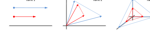
Figure 1: Visualization of optimal (blue) and suboptimal (red) $d$-rows in up to three dimensions. The vectors are individual rows in a $d$-row. The volume corresponding to the $d$-row is marked with dotted lines.

Based on our assumption, $(i^{\ast},j^{\ast})\in I^{\ast}\times J^{\ast}$. The claim that $i^{\ast}\in I^{\ast}$ follows from the observation that for any column $j$,

$$\max_{i\in[K]}U(i,:)V(j,:)^{\mathsf{\scriptscriptstyle T}}\leq\max_{z\in\mathcal{S}_{d}}zU^{\ast}V(j,:)^{\mathsf{\scriptscriptstyle T}}=\max_{k\in[d]}U^{\ast}(k,:)V(j,:)^{\mathsf{\scriptscriptstyle T}}\,.$$

The claim that $j^{\ast}\in J^{\ast}$ is proved analogously.

2.2 Simplified Problem

Our second key assumption is that we study a related problem to (1), learning of $(I^{\ast},J^{\ast})$. When $(I^{\ast},J^{\ast})$ is known, learning of $(i^{\ast},j^{\ast})$ is a problem with $d^{2}$ arms, which is small in comparison to our original problem with $KL$ arms. The learning agent interacts with our new problem as follows. At time $t$, the agent chooses arm $(\mathbf{I}_{t},\mathbf{J}_{t})\in\Pi_{d}([K])\times\Pi_{d}([L])$, a pair of $d$-subsets of rows and columns, and observes a noisy realization of matrix $\bar{R}(\mathbf{I}_{t},\mathbf{J}_{t})$, $\mathbf{r}_{t}(i,j)$ for all $(i,j)\in\mathbf{I}_{t}\times\mathbf{J}_{t}$. The reward is $\mathbf{r}_{t}(i^{\ast}(\mathbf{I}_{t},\mathbf{J}_{t}),j^{\ast}(\mathbf{I}_{t},\mathbf{J}_{t}))$, where

$$(i^{\ast}(I,J),j^{\ast}(I,J))=\operatorname*{arg\,max\,}_{(i,j)\in I\times J}\bar{R}(i,j)$$

for any $(I,J)\in\Pi_{d}([K])\times\Pi_{d}([L])$. To simplify language, we refer to the $d$-subsets of rows and columns as a $d$-row and $d$-column, respectively.

The objective of the learning agent is to minimize its expected cumulative regret in $n$ steps $\mathcal{R}(n)=\mathbb{E}\left[\sum_{t=1}^{n}\mathcal{R}(\mathbf{I}_{t},\mathbf{J}_{t})\right]$, where $\mathcal{R}(\mathbf{I}_{t},\mathbf{J}_{t})=\mathbf{r}_{t}(i^{\ast},j^{\ast})-\mathbf{r}_{t}(i^{\ast}(\mathbf{I}_{t},\mathbf{J}_{t}),j^{\ast}(\mathbf{I}_{t},\mathbf{J}_{t}))$ is the instantaneous stochastic regret of the agent at time $t$.

3 Noise-Free Problem

This section shows that the problem of finding the maximum entry of a noise-free low-rank matrix can be viewed as an elimination problem. We focus on row elimination. The column elimination is analogous. We start with rank-$1$ matrices. The maximum entry of a non-negative rank-$1$ matrix is in the row with the highest latent value [8]. Therefore, row $i$ can be eliminated by row $i^{\prime}$ when $U(i,1)<U(i^{\prime},1)$, when the length of $U(i,:)$ is lower than the length of $U(i^{\prime},:)$ (Figure 1a).

A natural generalization of the length in a one-dimensional space is the area in a two-dimensional space. Therefore, in our class of rank-$2$ matrices, a pair of rows $I\in\Pi_{2}([K])$ can be eliminated by a pair of rows $I^{\prime}\in\Pi_{2}([K])$ when the simplex over the rows of $U(I,:)$ has a smaller area than that over the rows of $U(I^{\prime},:)$, as shown in Figure 1b. This follows from our assumption that any $U(I,:)$ can be written as $U(I,:)=ZU^{\ast}$ for some $Z\in\mathcal{S}_{d,d}$.

Generally, in any rank-$d$ matrix in our class of matrices, a $d$-row $I$ can be eliminated by a $d$-row $I^{\prime}$ when the simplex over the rows of $U(I,:)$ has a smaller volume than that over the rows of $U(I^{\prime},:)$, as shown in Figure 1c. The volume of the simplex over the rows of $U(I,:)$ is $d!^{-1}\left|\operatorname{det}(U(I,:))\right|$. In the rest of this work, we neglect the factor of $d!$. This has no impact on elimination because this factor is common among all simplex volumes.

Unfortunately, the above approach cannot be implemented because $U$ is not observed, as we only observe the entries of $\bar{R}$. Therefore, we estimate $\left|\operatorname{det}(U(I,:))\right|$ from $\bar{R}(I,J)$, where $\bar{R}(I,J)$ are the observations of $d$-row $I\in\Pi_{d}([K])$ over $d$-column $J\in\Pi_{d}([L])$. In particular, from the definition of $\bar{R}$ and the properties of the determinant,

$$\operatorname{det}(\bar{R}(I,J))=\operatorname{det}(U(I,:)V(J,:)^{\mathsf{\scriptscriptstyle T}})=\operatorname{det}(U(I,:))\operatorname{det}(V(J,:))$$

for any $I\in\Pi_{d}([K])$ and $J\in\Pi_{d}([L])$. This implies that $\operatorname{det}(\bar{R}(I,J))$ can be viewed as a scaled observation of $\operatorname{det}(U(I,:))$; and that

$$\operatorname{det}^{2}(\bar{R}(I,J))<\operatorname{det}^{2}(\bar{R}(I^{\prime},J))\implies\operatorname{det}^{2}(U(I,:))<\operatorname{det}^{2}(U(I^{\prime},:))$$

for any $d$-rows $I$ and $I^{\prime}$, as long as $\operatorname{det}^{2}(V(J,:))>0$.

Algorithm 1 Finding the maximum entry of a noise-free rank-$d$ matrix.

1:Choose any $d$-column, $J_{1}\in\Pi_{d}([L])$, and observe it in all rows

2:Choose any $d$-row, $I_{1}\in\Pi_{d}([K])$, and observe it in all columns

3:

4:$I^{\ast}\leftarrow[d]$ $\triangleright$ Row elimination

5:for all $I\in\Pi_{d}([K])$ do

6:     if $\operatorname{det}^{2}(\bar{R}(I,J_{1}))>\operatorname{det}^{2}(\bar{R}(I^{\ast},J_{1}))$ then $I^{\ast}\leftarrow I$      

7:$J^{\ast}\leftarrow[d]$ $\triangleright$ Column elimination

8:for all $J\in\Pi_{d}([L])$ do

9:     if $\operatorname{det}^{2}(\bar{R}(I_{1},J))>\operatorname{det}^{2}(\bar{R}(I_{1},J^{\ast}))$ then $J^{\ast}\leftarrow J$      

The above reasoning leads to a particularly simple algorithm for solving the noise-free variant of our problem, which is presented in Algorithm 1. The algorithm is guaranteed to identify $(I^{\ast},J^{\ast})$ under the assumption that the minimum volume

$$c_{\min}=\min\left\{\min_{I\in\Pi_{d}([K])}\operatorname{det}^{2}(U(I,:)),\ \min_{J\in\Pi_{d}([L])}\operatorname{det}^{2}(V(J,:))\right\}$$ (2)

is positive. This means that any $d$ rows and columns of $\bar{R}$ are linearly independent. We discuss how to alleviate the dependence on $c_{\min}$ in Section 5.3.

4 Noisy Problem

Algorithm 1 is expected to perform poorly in the noisy setting. The challenge is that a single noisy realization of $\bar{R}(:,J_{1})$ and $\bar{R}(I_{1},:)$ is unlikely to be sufficient to learn $I^{\ast}$ and $J^{\ast}$. This issue can be addressed by observing multiple noisy realizations of $\bar{R}(:,J_{1})$ and $\bar{R}(I_{1},:)$, and then acting on their empirical averages. This approach is problematic for two reasons. First and foremost, when $I_{1}$ and $J_{1}$ are chosen poorly, $\operatorname{det}^{2}(U(I_{1},:))$ and $\operatorname{det}^{2}(V(J_{1},:))$ are close to zero, and many observations are needed to learn $I^{\ast}$ and $J^{\ast}$. Second, it is wasteful in the sense that some $d$-rows and $d$-columns can be detected as suboptimal from much less observations than the others. We propose an adaptive elimination algorithm that addresses these challenges in the next section.

4.1 Algorithm ${\tt LowRankElim}$

We propose an elimination algorithm [2] for finding the maximum entry of a noisy low-rank matrix, which maintains ${\tt UCB1}$ confidence intervals [1] on the scaled volumes of all $d$-rows and $d$-columns. The algorithm is presented in Algorithm 2 and we call it ${\tt LowRankElim}$. The algorithm operates in stages, which quadruple in length. In each stage, ${\tt LowRankElim}$ explores all remaining rows and columns randomly over all remaining $d$-columns and $d$-rows, respectively. At the end of the stage, it eliminates all $d$-rows and $d$-columns that cannot be optimal with a high probability. We denote the remaining $d$-rows and $d$-columns in stage $\ell$ by $\mathbf{A}^{\textsc{u}}_{\ell}$ and $\mathbf{A}^{\textsc{v}}_{\ell}$, respectively. The row and column variables are distinguished by their upper indices, which are u and v, respectively.

Algorithm 2 ${\tt LowRankElim}$ for finding the maximum entry of a noisy rank-$d$ matrix.

1:$\tilde{\Delta}_{0}\leftarrow 1$,  $\mathbf{A}^{\textsc{u}}_{0}\leftarrow\Pi_{d}([K])$,  $\mathbf{A}^{\textsc{v}}_{0}\leftarrow\Pi_{d}([L])$ $\triangleright$ Initialization

2:

3:for $\ell=0,1,\dots$ do

4:     $n_{\ell}\leftarrow\left\lceil 4\tilde{\Delta}_{\ell}^{-2}C(n)\right\rceil$

5:

6:     for $t=1,\dots,n_{\ell}$ do

7:         Choose random $d$-row $\mathbf{I}_{t}\in\mathbf{A}^{\textsc{u}}_{\ell}$ and $d$-column $\mathbf{J}_{t}\in\mathbf{A}^{\textsc{v}}_{\ell}$

8:         for $k=1,2$ do

9:              for all $i\in\bigcup_{I\in\mathbf{A}^{\textsc{u}}_{\ell}}I$ do $\triangleright$ Row exploration

10:                  Choose any $d$-row $I\in\mathbf{A}^{\textsc{u}}_{\ell}$ such that $i\in I$

11:                  Observe $d$-row $I$ over $\mathbf{J}_{t}$ and store it in $\mathbf{R}^{\textsc{u}}_{\ell,t,k}(I,:)$               

12:              for all $j\in\bigcup_{J\in\mathbf{A}^{\textsc{v}}_{\ell}}J$ do $\triangleright$ Column exploration

13:                  Choose any $d$-column $J\in\mathbf{A}^{\textsc{v}}_{\ell}$ such that $j\in J$

14:                  Observe $d$-column $J$ over $\mathbf{I}_{t}$ and store it in $\mathbf{R}^{\textsc{v}}_{\ell,t,k}(J,:)$                             

15:

16:     $\delta_{\ell}\leftarrow\sqrt{C(n)n_{\ell}^{-1}}$

17:     for all $I\in\mathbf{A}^{\textsc{u}}_{\ell}$ do $\triangleright$ UCBs and LCBs of all remaining $d$-rows

18:         $\hat{\mathbf{\mu}}^{\textsc{u}}_{\ell}(I)\leftarrow n_{\ell}^{-1}\sum_{t=1}^{n_{\ell}}\operatorname{det}(\mathbf{R}^{\textsc{u}}_{\ell,t,1}(I,:))\operatorname{det}(\mathbf{R}^{\textsc{u}}_{\ell,t,2}(I,:))$

19:         $\mathbf{U}^{\textsc{u}}_{\ell}(I)\leftarrow\hat{\mathbf{\mu}}^{\textsc{u}}_{\ell}(I)+\delta_{\ell}$,  $\mathbf{L}^{\textsc{u}}_{\ell}(I)\leftarrow\hat{\mathbf{\mu}}^{\textsc{u}}_{\ell}(I)-\delta_{\ell}$      

20:     for all $J\in\mathbf{A}^{\textsc{v}}_{\ell}$ do $\triangleright$ UCBs and LCBs of all remaining $d$-columns

21:         $\hat{\mathbf{\mu}}^{\textsc{v}}_{\ell}(J)\leftarrow n_{\ell}^{-1}\sum_{t=1}^{n_{\ell}}\operatorname{det}(\mathbf{R}^{\textsc{v}}_{\ell,t,1}(J,:))\operatorname{det}(\mathbf{R}^{\textsc{v}}_{\ell,t,2}(J,:))$

22:         $\mathbf{U}^{\textsc{v}}_{\ell}(J)\leftarrow\hat{\mathbf{\mu}}^{\textsc{v}}_{\ell}(J)+\delta_{\ell}$,  $\mathbf{L}^{\textsc{v}}_{\ell}(J)\leftarrow\hat{\mathbf{\mu}}^{\textsc{v}}_{\ell}(J)-\delta_{\ell}$      

23:

24:     $\mathbf{A}^{\textsc{u}}_{\ell+1}\leftarrow\mathbf{A}^{\textsc{u}}_{\ell}$,  $\mathbf{I}^{\ast}_{\ell}\leftarrow\operatorname*{arg\,max\,}_{I\in\mathbf{A}^{\textsc{u}}_{\ell}}\mathbf{L}^{\textsc{u}}_{\ell}(I)$ $\triangleright$ $d$-row elimination

25:     for all $I\in\mathbf{A}^{\textsc{u}}_{\ell}$ do

26:         if $\mathbf{U}^{\textsc{u}}_{\ell}(I)\leq\mathbf{L}^{\textsc{u}}_{\ell}(\mathbf{I}^{\ast}_{\ell})$ then $\mathbf{A}^{\textsc{u}}_{\ell+1}\leftarrow\mathbf{A}^{\textsc{u}}_{\ell+1}\setminus\left\{I\right\}$               

27:     $\mathbf{A}^{\textsc{v}}_{\ell+1}\leftarrow\mathbf{A}^{\textsc{v}}_{\ell}$,  $\mathbf{J}^{\ast}_{\ell}\leftarrow\operatorname*{arg\,max\,}_{J\in\mathbf{A}^{\textsc{v}}_{\ell}}\mathbf{L}^{\textsc{v}}_{\ell}(J)$ $\triangleright$ $d$-column elimination

28:     for all $J\in\mathbf{A}^{\textsc{v}}_{\ell}$ do

29:         if $\mathbf{U}^{\textsc{v}}_{\ell}(J)\leq\mathbf{L}^{\textsc{v}}_{\ell}(\mathbf{J}^{\ast}_{\ell})$ then $\mathbf{A}^{\textsc{v}}_{\ell+1}\leftarrow\mathbf{A}^{\textsc{v}}_{\ell+1}\setminus\left\{J\right\}$               

30:

31:     $\tilde{\Delta}_{\ell+1}\leftarrow\tilde{\Delta}_{\ell}/2$

Each stage of Algorithm 2 has three main steps: exploration, estimation, and elimination. In the exploration step (lines $4$–$12$), all remaining rows and columns are explored over $n_{\ell}$ random remaining $d$-columns and $d$-rows, respectively. The row and column observations are stored in matrices $\mathbf{R}^{\textsc{u}}_{\ell,t,k}\in\mathbb{R}^{K\times d}$ and $\mathbf{R}^{\textsc{v}}_{\ell,t,k}\in\mathbb{R}^{L\times d}$, respectively. Therefore, the maximum number of observations in stage $\ell$ is $2(K+L)d^{2}n_{\ell}$. The separation of row and column observations is necessary to guarantee that the row and column estimators are scaled by the same factor, as in Section 3.

In the estimation step (lines $13$–$19$), ${\tt LowRankElim}$ estimates high-probability upper and lower confidence bounds on the scaled volumes of all remaining $d$-rows and $d$-columns. The scaled volume of $d$-row $I\in\mathbf{A}^{\textsc{u}}_{\ell}$ is estimated as $\hat{\mathbf{\mu}}^{\textsc{u}}_{\ell}(I)$ in line $13$. Since $\mathbf{R}^{\textsc{u}}_{\ell,t,1}(I,:)$ and $\mathbf{R}^{\textsc{u}}_{\ell,t,2}(I,:)$ are independent noisy observations of $\bar{R}(I,\mathbf{J}_{t})$, it is easy to show that

$$\mathbb{E}\left[\hat{\mathbf{\mu}}^{\textsc{u}}_{\ell}(I)\right]=\left|\mathbf{A}^{\textsc{v}}_{\ell}\right|^{-1}\sum_{J\in\mathbf{A}^{\textsc{v}}_{\ell}}\operatorname{det}^{2}(\bar{R}(I,J))$$

for any remaining $d$-columns $\mathbf{A}^{\textsc{v}}_{\ell}$. Also note that any realization of $\operatorname{det}(\mathbf{R}^{\textsc{u}}_{\ell,t,k}(I,:))$ is reasonably bounded for small $d$. In particular, let $\operatorname{det}_{\max}(d)=\max_{M\in[0,1]^{d\times d}}\operatorname{det}(M)$ be the maximum determinant of a $d\times d$ matrix on $[0,1]$. Then $\left|\operatorname{det}(\mathbf{R}^{\textsc{u}}_{\ell,t,k}(I,:))\right|\leq\operatorname{det}_{\max}(d)$, where $\operatorname{det}_{\max}(d)$ is $1$, $1$, $2$, and $3$ when $d$ is $1$, $2$, $3$, and $4$, respectively. Therefore, when $d$ is small, we can argue that $\hat{\mathbf{\mu}}^{\textsc{u}}_{\ell}(I)$ concentrates at $\bar{\mathbf{\mu}}^{\textsc{u}}_{\ell}(I)$ by standard concentration inequalities for bounded i.i.d. random variables.

In the elimination step (lines $20$–$25$), ${\tt LowRankElim}$ eliminates suboptimal $d$-rows and $d$-columns. The confidence intervals are designed such that $\mathbf{U}^{\textsc{u}}_{\ell}(I)\leq\mathbf{L}^{\textsc{u}}_{\ell}(\mathbf{I}^{\ast}_{\ell})$ implies that $d$-row $I$ is suboptimal with a high probability for any column elimination policy up to the end of stage $\ell$, and $\mathbf{U}^{\textsc{v}}_{\ell}(J)\leq\mathbf{L}^{\textsc{v}}_{\ell}(\mathbf{J}^{\ast}_{\ell})$ implies that $d$-column $J$ is suboptimal with a high probability for any row elimination policy up to the end of stage $\ell$. As a result, all eliminations are correct with a high probability.

The computational complexity of the estimation and elimination steps (lines $13$–$25$) is exponential in $d$. Therefore, they can be implemented efficiently only for small $d$. The confidence radii depend on $\log n$ through

$$C(n)=4\operatorname{det}_{\max}^{2}(d)\log((K^{d}+L^{d})n)\,.$$ (3)

Since $K^{d}+L^{d}\leq(K+L)^{d}$, $C(n)$ is at most linear in $d$.

5 Analysis

This section has three parts. In Section 5.1, we present a gap-dependent upper bound on the $n$-step regret of ${\tt LowRankElim}$. In Section 5.2, we state our key lemmas and sketch their proofs. In Section 5.3, we discuss the results of our analysis.

5.1 Upper Bound

${\tt LowRankElim}$ seems to be a reasonable generalization of Algorithm 1 to the noisy setting, where the scaled estimates of volumes are substituted with their upper and lower confidence bounds. As a result, it is expected that ${\tt LowRankElim}$ eliminates all suboptimal $d$-rows and $d$-columns as the number of stages increases, as long as all confidence bounds hold with a high probability. In this section, we derive a finite-time upper bound on the regret of ${\tt LowRankElim}$.

We measure the regret of ${\tt LowRankElim}$ by several metrics. Let $I\in\Pi_{d}([K])$ be suboptimal $d$-row and $J\in\Pi_{d}([L])$ be suboptimal $d$-column. Then the gaps of $d$-row $I$ and $d$-column $J$,

$$\Delta^{\textsc{u}}_{I}=\operatorname{det}^{2}(U(I^{\ast},:))-\operatorname{det}^{2}(U(I,:))\,,\quad\Delta^{\textsc{v}}_{J}=\operatorname{det}^{2}(V(J^{\ast},:))-\operatorname{det}^{2}(V(J,:))\,,$$

measure the hardness of eliminating $I$ and $J$ under the assumption that $U$ and $V$ are known. We define the minimum gap as the minimum of the $d$-row and $d$-column gaps,

$$\Delta_{\min}=\min\left\{\min_{I\in\Pi_{d}([K])\setminus\left\{I^{\ast}\right\}}\Delta^{\textsc{u}}_{I},\ \min_{J\in\Pi_{d}([L])\setminus\left\{J^{\ast}\right\}}\Delta^{\textsc{u}}_{J}\right\}\,.$$ (4)

However, $U$ and $V$ are not known, and therefore ${\tt LowRankElim}$ estimates scaled volumes of $d$-rows and $d$-columns. The penalty for estimating scaled volumes is reflected by the minimum volume $c_{\min}$ in (2) and the maximum volume

$$c_{\max}=\min\left\{\operatorname{det}^{2}(U^{\ast}),\ \operatorname{det}^{2}(V^{\ast})\right\}\,.$$ (5)

Note that $c_{\min}>0$ implies that any $d$ rows and columns of $\bar{R}$ are linearly independent. We discuss how to eliminate the dependence on $c_{\min}$ in Section 5.3. Our main theorem is stated below.

Theorem 1.

The expected $n$-step regret of ${\tt LowRankElim}$ is bounded as

$$\mathcal{R}(n)\leq\frac{cd^{3}(K+L)}{c_{\max}c_{\min}^{2}\Delta_{\min}}C(n)+4\,,$$

where $c=3072$, $c_{\max}$ is defined in (5), $c_{\min}$ is defined in (2), $\Delta_{\min}$ is defined in (4), and $C(n)$ is defined in (3).

Proof.

Let $m$ be the first stage such that all suboptimal $d$-rows and $d$-columns are eliminated by its end, $\tilde{\Delta}_{m}<c_{\min}\Delta_{\min}/2$. Let $\mathcal{R}_{\ell}$ be the expected regret of ${\tt LowRankElim}$ in stage $\ell$ under event $\mathcal{E}$. Then the expected $n$-step regret of ${\tt LowRankElim}$ is bounded as

$$\mathcal{R}(n)\leq\mathbb{E}\left[\mathcal{R}(n)\mathds{1}\!\left\{\mathcal{E}\right\}\right]+nP(\overline{\mathcal{E}})\leq\mathbb{E}\left[\mathcal{R}(n)\mathds{1}\!\left\{\mathcal{E}\right\}\right]+4\leq\sum_{\ell=0}^{m}\mathcal{R}_{\ell}+4\,,$$

where the second inequality is from $P(\overline{\mathcal{E}})\leq 4n^{-1}$ (Lemma 1) and the last inequality holds because all suboptimal $d$-rows and $d$-columns are eliminated after stage $m$ (Lemma 3).

When $d$-row $I$ or $d$-column $J$ is active in stage $\ell$, it has not been eliminated in the previous stages. Therefore, by Lemma 3, $c_{\min}\Delta^{\textsc{u}}_{I}\leq 2\tilde{\Delta}_{\ell-1}=4\tilde{\Delta}_{\ell}$ and $c_{\min}\Delta^{\textsc{v}}_{J}\leq 2\tilde{\Delta}_{\ell-1}=4\tilde{\Delta}_{\ell}$. Furthermore, by the design of exploration in ${\tt LowRankElim}$ (lines $4$–$12$), each remaining row and column is explored in some remaining $I$ and $J$, respectively, that contains it. Therefore, by the regret decomposition in Lemma 2, the $n$-step regret is bounded from above as

$$\sum_{\ell=0}^{m}\mathcal{R}_{\ell}\leq 2\sum_{\ell=0}^{m}\frac{6d^{3}(4\tilde{\Delta}_{\ell}+4\tilde{\Delta}_{\ell})}{c_{\max}c_{\min}}(K+L)n_{\ell}=\frac{96d^{3}(K+L)}{c_{\max}c_{\min}}\sum_{\ell=0}^{m}\tilde{\Delta}_{\ell}n_{\ell}\,.$$

The additional factor of $2$ is because ${\tt LowRankElim}$ explores everything twice. Note that the above upper bound is only possible because $d$-rows and $d$-columns are eliminated simultaneously.

Now we express $n_{\ell}$ and note that $\tilde{\Delta}_{m}=\tilde{\Delta}_{m-1}/2\geq c_{\min}\Delta_{\min}/4$ from the definition of $m$,

$$\sum_{\ell=0}^{m}\tilde{\Delta}_{\ell}n_{\ell}\leq 4C(n)\sum_{\ell=0}^{m}\frac{1}{\tilde{\Delta}_{\ell}}=\frac{4}{\tilde{\Delta}_{m}}C(n)\sum_{\ell=0}^{m}2^{-\ell}\leq\frac{32}{c_{\min}\Delta_{\min}}C(n)\,.$$

Finally, we chain all above inequalities and get our main claim.  

5.2 Key Lemmas

We state our key lemmas below, together with sketches of their proofs.

Lemma 1.

Let

$$\bar{\mathbf{\mu}}^{\textsc{u}}_{\ell}(I)=\left|\mathbf{A}^{\textsc{v}}_{\ell}\right|^{-1}\sum_{J\in\mathbf{A}^{\textsc{v}}_{\ell}}\operatorname{det}^{2}(\bar{R}(I,J))\,,\quad\bar{\mathbf{\mu}}^{\textsc{v}}_{\ell}(J)=\left|\mathbf{A}^{\textsc{u}}_{\ell}\right|^{-1}\sum_{I\in\mathbf{A}^{\textsc{u}}_{\ell}}\operatorname{det}^{2}(\bar{R}(I,J))$$

be the expected scaled volumes of $d$-row $I$ and $d$-column $J$ in stage $\ell$, and let

$$\mathcal{E}^{\textsc{u}}_{\ell,I}=\left\{\bar{\mathbf{\mu}}^{\textsc{u}}_{\ell}(I)\in[\mathbf{L}^{\textsc{u}}_{\ell}(I),\mathbf{U}^{\textsc{u}}_{\ell}(I)]\right\}\,,\quad\mathcal{E}^{\textsc{v}}_{\ell,J}=\left\{\bar{\mathbf{\mu}}^{\textsc{v}}_{\ell}(J)\in[\mathbf{L}^{\textsc{v}}_{\ell}(J),\mathbf{U}^{\textsc{v}}_{\ell}(J)]\right\}$$

be the events that the confidence intervals on these expected volumes hold. Let $\mathcal{E}$ be the event that all confidence intervals hold and $\overline{\mathcal{E}}$ be the complement of this event. Then $P(\overline{\mathcal{E}})\leq 4n^{-1}$.

Proof.

First, we prove that $\mathbb{E}\left[\hat{\mathbf{\mu}}^{\textsc{u}}_{\ell}(I)\right]=\bar{\mathbf{\mu}}^{\textsc{u}}_{\ell}(I)$ and $\hat{\mathbf{\mu}}^{\textsc{u}}_{\ell}(I)\in[0,\operatorname{det}_{\max}^{2}(d)]$ for any stage $\ell$, $d$-row $I\in\Pi_{d}([K])$, and remaining $d$-columns $\mathbf{A}^{\textsc{v}}_{\ell}$ in stage $\ell$. Therefore, we can argue that $\hat{\mathbf{\mu}}^{\textsc{u}}_{\ell}(I)$ is close to $\bar{\mathbf{\mu}}^{\textsc{u}}_{\ell}(I)$ by Hoeffding’s inequality. The column argument is analogous. Finally, by the union bound, we argue that it is unlikely that $\hat{\mathbf{\mu}}^{\textsc{u}}_{\ell}(I)$ and $\hat{\mathbf{\mu}}^{\textsc{v}}_{\ell}(J)$ are not close to $\bar{\mathbf{\mu}}^{\textsc{u}}_{\ell}(I)$ and $\bar{\mathbf{\mu}}^{\textsc{v}}_{\ell}(J)$, respectively, in any stage $\ell$. The complete proof is in Appendix A.  

Lemma 2.

Let $I$ and $J$ be any $d$-row and $d$-column, respectively. Then

$$\bar{R}(i^{\ast},j^{\ast})-\bar{R}(i^{\ast}(I,J),j^{\ast}(I,J))\leq 6d^{3}\frac{\Delta^{\textsc{u}}_{I}+\Delta^{\textsc{v}}_{J}}{c_{\max}}\,.$$

Proof.

First, we bound the regret from above by the differences in its row and column components, $U^{\ast}-U(I,:)$ and $V^{\ast}-V(J,:)$. Then we argue that $U^{\ast}-U(I,:)$ can be bounded as a function of $\operatorname{det}^{2}(U^{\ast})-\operatorname{det}^{2}(U(I,:))$, which is proved in Lemma 4 in Appendix D. The column argument is analogous. The complete proof is in Appendix B.  

Lemma 3.

Let event $\mathcal{E}$ happen and $m$ be the first stage where $\tilde{\Delta}_{m}<c_{\min}\Delta^{\textsc{u}}_{I}/2$, where $c_{\min}$ is defined in (2). Then $d$-row $I$ is guaranteed to be eliminated by the end of stage $m$. Moreover, let $m$ be the first stage where $\tilde{\Delta}_{m}<c_{\min}\Delta^{\textsc{v}}_{J}/2$. Then $d$-column $J$ is guaranteed to be eliminated by the end of stage $m$.

Proof.

From the definition of our confidence intervals in ${\tt LowRankElim}$, $\mathbf{U}^{\textsc{u}}_{\ell}(I)<\mathbf{L}^{\textsc{u}}_{\ell}(I^{\ast})$ happens when $2\tilde{\Delta}_{m}\leq\bar{\mathbf{\mu}}^{\textsc{u}}_{\ell}(I^{\ast})-\bar{\mathbf{\mu}}^{\textsc{u}}_{\ell}(I)$. Now note that $\bar{\mathbf{\mu}}^{\textsc{u}}_{\ell}(I^{\ast})-\bar{\mathbf{\mu}}^{\textsc{u}}_{\ell}(I)$ is bounded from below by $c_{\min}\Delta^{\textsc{u}}_{I}$. The column argument is analogous. The complete proof is in Appendix C.  

5.3 Discussion

We derive a gap-dependent upper bound on the $n$-step regret of ${\tt LowRankElim}$ in Theorem 1. The bound does not depend on $KL$; is linear in the reciprocal of the minimum gap $\Delta_{\min}$ in (4) and logarithmic in $n$ through $C(n)$ in (3). To the best of our knowledge, ${\tt LowRankElim}$ is the first algorithm that achieves such regret. The polynomial dependence on rank $d$ is suboptimal and we believe that it can be reduced by a more elaborate analysis. The goal of our work is not to conduct such an analysis, but to demonstrate that these kinds of bounds are attainable by bandit algorithms.

Our regret bound also depends on the reciprocal of two problem-dependent quantities, $c_{\max}$ in (5) and $c_{\min}$ in (2), which do not depend on $K$, $L$, $\Delta_{\min}$, and $n$. The maximum volume $c_{\max}$ arises in Lemma 4 in Appendix D, which relates volume to regret. This quantity is not critical because it is unlikely to be small. In fact, $c_{\max}\geq c_{\min}$ by definition. The minimum volume $c_{\min}$ is the penalty for estimating scaled volumes of $d$-rows and $d$-columns, over random $d$-columns and $d$-rows, respectively. This is a form of averaging. Therefore, $c_{\min}$ is expected to be proportional to some notion of an average determinant, and not the minimum determinant as in (2).

In the rest of this section, we suggest a modification of ${\tt LowRankElim}$ whose regret scales much better with the minimum volume. The key idea is to follow Katariya et al. [8] and slightly change the exploration step. The change is to choose the $d$-rows and $d$-columns in line $5$ of ${\tt LowRankElim}$ randomly from $\Pi_{d}([K])$ and $\Pi_{d}([L])$, respectively. If the chosen $d$-row is eliminated in an earlier stage, it is replaced with the $d$-row that eliminated it; or the $d$-row that eliminated the earlier eliminating $d$-row, and so on. The same strategy is applied to $d$-columns. The result is that the averaging penalty does not worsen with elimination. Then $c_{\min}$ in Lemma 3 can be substituted with $\bar{c}=\exp[\min\left\{\bar{c}_{\textsc{u}},\bar{c}_{\textsc{v}}\right\}]$, where

$$\bar{c}_{\textsc{u}}=\left|\Pi_{d}([K])\right|^{-1}\sum_{I\in\Pi_{d}([K])}\operatorname{det}^{2}(U(I,:))\,,\quad\bar{c}_{\textsc{v}}=\left|\Pi_{d}([L])\right|^{-1}\sum_{J\in\Pi_{d}([L])}\operatorname{det}^{2}(V(J,:))\,;$$

and the expected $n$-step regret of ${\tt LowRankElim}$ becomes

$$\mathcal{R}(n)\leq\frac{cd^{3}(K+L)}{c_{\max}\bar{c}^{2}\Delta_{\min}}C(n)+4\,.$$

6 Related Work

The closest related paper to our work are stochastic rank-$1$ bandits of Katariya et al. [8]. This work can be viewed as a generalization of rank-$1$ bandits to a higher rank. Although our algorithm and analysis are motivated by Katariya et al. [8], our generalization is highly non-trivial. For instance, it is easy to see that the maximum entry of a non-negative rank-$1$ lies in its row and column with highest latent values. This is not true when the rank $d>1$. Therefore, it may seem that the work of Katariya et al. [8] cannot be generalized to a higher rank; and even if, it is unclear under what assumptions. We not only generalize this work, but also recover similar regret dependence.

Several papers studied various forms of low-rank matrix completion in the bandit setting. Zhao et al. [17] proposed a bandit algorithm for low-rank matrix completion, where the distribution over latent item factors is approximated by a point estimate. The algorithm is not analyzed. Kawale et al. [9] proposed a Thompson sampling algorithm for low-rank matrix completion, where the distribution over low-rank matrices is approximated by particle filtering. A computationally-inefficient variant of the algorithm has $O(\Delta^{-2}\log n)$ regret in rank-$1$ matrices. Sen et al. [16] proposed an $\varepsilon$-greedy algorithm for non-negative matrix completion. Its regret is $O(\Delta^{-2}\log n)$ and its analysis relies on a variant of the restricted isometry property, which may be hard to satisfy in practice. The following three papers studied clustering in the bandit setting, which is a form of a low-rank structure. Gentile et al. [7] clustered users based on their preferences, under the assumption that the features of items are known. Li et al. [12] generalized this algorithm to the clustering of items. Maillard et al. [13] studied a multi-armed bandit problem where the arms are partitioned into latent groups. All above papers also differ from our work in the setting. Our learning agent chooses both the row and column. In all above papers, the nature chooses the row.

Bhargava et al. [3] studied active matrix completion of positive semi-definite matrices and discussed its applications to bandits. This work is not comparable to our paper because the classes of completed matrices are different.

Matrix recovery and completion have been studied extensively in both machine learning and statistics [5, 10, 4, 11]. A good recent review of the prior work is Davenport and Romberg [6]. The existing guarantees in noisy matrix completion are unsuitable for our setting because they are on $\|\bar{R}-\hat{R}\|_{F}$, where $\bar{R}\in[0,1]^{K\times L}$ is the unobserved matrix and $\hat{R}\in[0,1]^{L\times K}$ is its recovered approximation. For the sake of concreteness, suppose that the noise is $\mathcal{N}(0,1)$. Then, by Theorem 7 in Candes and Plan [4], $\|\bar{R}-\hat{R}\|_{F}\leq\sqrt{\max\left\{K,L\right\}}$ at best. This bound is not sufficient for our purpose, because the gap between the highest and second highest entries of $\bar{R}$ is by definition smaller than $1$. In fact, many entries of the matrix may need to be observed many times to learn its maximum entry, as this may not be possible from observing only a small portion of the matrix.

7 Conclusions

We propose an algorithm for finding the maximum entry of a class of stochastic low-rank matrices, which we call ${\tt LowRankElim}$. ${\tt LowRankElim}$ is computationally and sample efficient when the rank of the matrix is small. We derive a gap-dependent upper bound on the $n$-step regret of our algorithm that does not depend on $KL$, the product of the number of rows $K$ and columns $L$ in the matrix. The bound is linear in the reciprocal of the minimum gap and logarithmic in the number of steps $n$. Although such bounds have become common in many bandit problems, we are unaware of any such bound in stochastic low-rank matrix completion. To the best of our knowledge, this paper presents the first such result. Note that our bound is proved without making any incoherence assumption on matrices, as is common in matrix completion [6]. This clearly indicates that the problem of learning the maximum entry of a matrix is fundamentally different from matrix completion.

We leave open several questions of interest. The strongest assumption in our work is that any row of $U$ and $V$ can be written as a convex combination of $d$ base rows and columns, respectively. We believe that this assumption can be relaxed. In particular, under the assumption that all entries of $U$ and $V$ are non-negative, the maximum entry of $\bar{R}=UV^{\mathsf{\scriptscriptstyle T}}$ at the vertices of the convex hulls over the rows of $U$ and $V$, respectively. These convex hulls are maximum volume convex objects in row and column latent spaces, similarly to $U^{\ast}$ and $V^{\ast}$ in Section 1. Therefore, we believe that they can be learned, at least in theory, by a similar algorithm to ${\tt LowRankElim}$.

Another limitation of our work is the dependence on rank $d$. The polynomial dependence on $d$ in our regret bound (Theorem 1) is likely to be suboptimal, and we believe that it can be reduced by a more elaborate analysis. In addition, ${\tt LowRankElim}$ is not computationally efficient when $d$ is large. We believe that it can be implemented computationally efficiently because our class of matrices can be factored using linear programming [14]. Finally, ${\tt LowRankElim}$ is not sample efficient when $d$ is large. We believe that our algorithm can be implemented sample efficiently if the distributions of the determinant products in ${\tt LowRankElim}$ are sub-Gaussian in $\operatorname{poly}(d)$. This may be possible because the expectations of the determinant products is in $[0,1]$.

Appendix A Proof of Lemma 1

Fix any stage $\ell$, $d$-row $I\in\Pi_{d}([K])$, and remaining $d$-columns $\mathbf{A}^{\textsc{v}}_{\ell}$ in stage $\ell$. Then

$$\operatorname{det}(\mathbf{R}^{\textsc{u}}_{\ell,t,1}(I,:))\operatorname{det}(\mathbf{R}^{\textsc{u}}_{\ell,t,2}(I,:))$$

is an i.i.d. random variable in $t$ with two properties. First, any of its realizations is bounded as

$$\operatorname{det}(\mathbf{R}^{\textsc{u}}_{\ell,t,1}(I,:))\operatorname{det}(\mathbf{R}^{\textsc{u}}_{\ell,t,2}(I,:))\leq\operatorname{det}_{\max}^{2}(d)$$

because both $\mathbf{R}^{\textsc{u}}_{\ell,t,1}(I,:)$ and $\mathbf{R}^{\textsc{u}}_{\ell,t,2}(I,:)$ are random $d\times d$ matrices on $[0,1]$. Second,

$$\mathbb{E}\left[\operatorname{det}(\mathbf{R}^{\textsc{u}}_{\ell,t,1}(I,:))\operatorname{det}(\mathbf{R}^{\textsc{u}}_{\ell,t,2}(I,:))\right] =\mathbb{E}\left[\mathbb{E}\left[\operatorname{det}(\mathbf{R}^{\textsc{u}}_{\ell,t,1}(I,:))\operatorname{det}(\mathbf{R}^{\textsc{u}}_{\ell,t,2}(I,:))\,\middle|\,\mathbf{J}_{t}\right]\right]$$

$$=\mathbb{E}\left[\mathbb{E}\left[\operatorname{det}(\mathbf{R}^{\textsc{u}}_{\ell,t,1}(I,:))\,\middle|\,\mathbf{J}_{t}\right]\mathbb{E}\left[\operatorname{det}(\mathbf{R}^{\textsc{u}}_{\ell,t,2}(I,:))\,\middle|\,\mathbf{J}_{t}\right]\right]$$

$$=\mathbb{E}\left[\operatorname{det}^{2}(\bar{R}(I,\mathbf{J}_{t})\right]$$

$$=\left|\mathbf{A}^{\textsc{v}}_{\ell}\right|^{-1}\sum_{J\in\mathbf{A}^{\textsc{v}}_{\ell}}\operatorname{det}^{2}(\bar{R}(I,J))$$

$$=\bar{\mathbf{\mu}}^{\textsc{u}}_{\ell}(I)\,,$$

where the first equality is from the tower rule, the second equality is from two independent observations of $\bar{R}(I,\mathbf{J}_{t})$, the third equality is because $\mathbb{E}\left[\operatorname{det}(\mathbf{Z})\right]=\operatorname{det}(\mathbb{E}\left[\mathbf{Z}\right])$ for any $\mathbf{Z}$ whose entries have independent noise, and the fourth equality is because $\mathbf{J}_{t}$ is chosen uniformly at random from $\mathbf{A}^{\textsc{v}}_{\ell}$. Therefore, by Hoeffding’s inequality and from the definition of $C(n)$ in (3),

$$P(\bar{\mathbf{\mu}}^{\textsc{u}}_{\ell}(I)\notin[\mathbf{L}^{\textsc{u}}_{\ell}(I),\mathbf{U}^{\textsc{u}}_{\ell}(I)]) =P\left(\left|\hat{\mathbf{\mu}}^{\textsc{u}}_{\ell}(I)-\bar{\mathbf{\mu}}^{\textsc{u}}_{\ell}(I)\right|\geq\sqrt{C(n)n_{\ell}^{-1}}\right)$$

$$\leq 2\exp[-2C(n)(2\operatorname{det}_{\max}(d))^{-2}]$$

$$\leq 2\exp[-2\log((K^{d}+L^{d})n)]$$

$$\leq 2K^{-d}n^{-2}\,.$$

By the same line of reasoning,

$$P(\bar{\mathbf{\mu}}^{\textsc{v}}_{\ell}(J)\notin[\mathbf{L}^{\textsc{v}}_{\ell}(J),\mathbf{U}^{\textsc{v}}_{\ell}(J)])\leq 2L^{-d}n^{-2}$$

for any stage $\ell$, $d$-column $J\in\Pi_{d}([L])$, and remaining $d$-rows $\mathbf{A}^{\textsc{u}}_{\ell}$ in stage $\ell$. Finally, by the union bound and from the above inequalities,

$$P(\overline{\mathcal{E}}) \leq\sum_{\ell=0}^{n-1}\sum_{I\in\Pi_{d}([K])}P(\bar{\mathbf{\mu}}^{\textsc{u}}_{\ell}(I)\notin[\mathbf{L}^{\textsc{u}}_{\ell}(I),\mathbf{U}^{\textsc{u}}_{\ell}(I)])+\sum_{\ell=0}^{n-1}\sum_{J\in\Pi_{d}([L])}P(\bar{\mathbf{\mu}}^{\textsc{v}}_{\ell}(J)\notin[\mathbf{L}^{\textsc{v}}_{\ell}(J),\mathbf{U}^{\textsc{v}}_{\ell}(J)])$$

$$\leq 4n^{-1}\,.$$

This concludes our proof.

Appendix B Proof of Lemma 2

Let $U=U(I,:)$ and $V=V(J,:)$. Fix any permutations $\pi^{\textsc{u}}$ and $\pi^{\textsc{v}}$ over $[d]$. Then the regret can be decomposed into its row and column components as

$$\bar{R}(i^{\ast},j^{\ast})-\bar{R}(i^{\ast}(I,J),j^{\ast}(I,J))$$

$$\quad=\max_{i,j\in[d]}U^{\ast}(i,:)V^{\ast}(j,:)^{\mathsf{\scriptscriptstyle T}}-\max_{i,j\in[d]}U(i,:)V(j,:)^{\mathsf{\scriptscriptstyle T}}$$

$$\quad=\max_{i,j\in[d]}U^{\ast}(i,:)V^{\ast}(j,:)^{\mathsf{\scriptscriptstyle T}}-\max_{i,j\in[d]}U(\pi^{\textsc{u}}(i),:)V^{\ast}(j,:)^{\mathsf{\scriptscriptstyle T}}+{}$$

$$\quad\hskip 11.92406pt\max_{i,j\in[d]}U(i,:)V^{\ast}(j,:)^{\mathsf{\scriptscriptstyle T}}-\max_{i,j\in[d]}U(i,:)V(\pi^{\textsc{v}}(j),:)^{\mathsf{\scriptscriptstyle T}}$$

$$\quad\leq\sum_{i,j=1}^{d}\left|(U^{\ast}(i,:)-U(\pi^{\textsc{u}}(i),:))V^{\ast}(j,:)^{\mathsf{\scriptscriptstyle T}}\right|+\sum_{i,j=1}^{d}\left|(V^{\ast}(i,:)-V(\pi^{\textsc{v}}(i),:))U(j,:)^{\mathsf{\scriptscriptstyle T}}\right|\,.$$ (6)

Now we focus on the first term. By definition, $U=ZU^{\ast}$ for some $Z\in\mathcal{S}_{d,d}$, and therefore

$$\sum_{i,j=1}^{d}\left|(U^{\ast}(i,:)-U(\pi^{\textsc{u}}(i),:))V^{\ast}(j,:)^{\mathsf{\scriptscriptstyle T}}\right|\leq\sum_{i=1}^{d}\left|E(i,:)-Z(\pi^{\textsc{u}}(i),:))\right|\sum_{j=1}^{d}\left|U^{\ast}V^{\ast}(j,:)^{\mathsf{\scriptscriptstyle T}}\right|\,,$$

where $E=I_{d}$. By the Cauchy-Schwarz inequality,

$$\sum_{i=1}^{d}\left|E(i,:)-Z(\pi^{\textsc{u}}(i),:))\right|\sum_{j=1}^{d}\left|U^{\ast}V^{\ast}(j,:)^{\mathsf{\scriptscriptstyle T}}\right| \leq\sum_{i=1}^{d}\left\|E(i,:)-Z(\pi^{\textsc{u}}(i),:)\right\|_{2}\Bigg{\|}\sum_{j=1}^{d}\left|U^{\ast}V^{\ast}(j,:)^{\mathsf{\scriptscriptstyle T}}\right|\Bigg{\|}_{2}$$

$$\leq d^{\frac{3}{2}}\sum_{i=1}^{d}\left\|E(i,:)-Z(\pi^{\textsc{u}}(i),:)\right\|_{2}\,.$$

Let $\pi^{\textsc{u}}$ be the permutation in Lemma 4. Then we apply the lemma and get that

$$d^{\frac{3}{2}}\sum_{i=1}^{d}\left\|E(i,:)-Z(i,:)\right\|_{2}\leq 6d^{3}(1-\operatorname{det}^{2}(Z))=6d^{3}\frac{\operatorname{det}^{2}(U^{\ast})-\operatorname{det}^{2}(U)}{\operatorname{det}^{2}(U^{\ast})}\,.$$

The second term in (6) can be bounded analogously as

$$\sum_{i,j=1}^{d}\left|(V^{\ast}(i,:)-V(\pi^{\textsc{v}}(i),:))U(j,:)^{\mathsf{\scriptscriptstyle T}}\right|\leq 6d^{3}\frac{\operatorname{det}^{2}(V^{\ast})-\operatorname{det}^{2}(V)}{\operatorname{det}^{2}(V^{\ast})}\,.$$

Now we put both upper bounds together and get that

$$\bar{R}(i^{\ast},j^{\ast})-\bar{R}(i^{\ast}(I,J),j^{\ast}(I,J))\leq 6d^{3}\frac{\Delta^{\textsc{u}}_{I}+\Delta^{\textsc{v}}_{J}}{\min\left\{\operatorname{det}^{2}(U^{\ast}),\ \operatorname{det}^{2}(V^{\ast})\right\}}\,.$$

This concludes our proof.

Appendix C Proof of Lemma 3

We only prove the first claim. The other claim can be proved analogously.

Let $\bar{\mathbf{\mu}}^{\textsc{u}}_{\ell}(I)$ and $\hat{\mathbf{\mu}}^{\textsc{u}}_{\ell}(I)$ be defined as in Lemma 1. Let $\bar{\mathbf{\mu}}^{\textsc{u}}_{\ell}(I^{\ast})$ and $\hat{\mathbf{\mu}}^{\textsc{u}}_{\ell}(I^{\ast})$ be the corresponding values for $I^{\ast}$. Then from the definition of our confidence intervals and that event $\mathcal{E}$ happens,

$$\mathbf{U}^{\textsc{u}}_{\ell}(I) \leq\hat{\mathbf{\mu}}^{\textsc{u}}_{\ell}(I)+\frac{\tilde{\Delta}_{m}}{2}\leq\bar{\mathbf{\mu}}^{\textsc{u}}_{\ell}(I)+\tilde{\Delta}_{m}\,,\quad$$

$$\mathbf{L}^{\textsc{u}}_{\ell}(I^{\ast}) \geq\hat{\mathbf{\mu}}^{\textsc{u}}_{\ell}(I^{\ast})-\frac{\tilde{\Delta}_{m}}{2}\geq\bar{\mathbf{\mu}}^{\textsc{u}}_{\ell}(I^{\ast})-\tilde{\Delta}_{m}\,.$$

To complete the proof, it remains to show that

$$\bar{\mathbf{\mu}}^{\textsc{u}}_{\ell}(I^{\ast})-\tilde{\Delta}_{m}-(\bar{\mathbf{\mu}}^{\textsc{u}}_{\ell}(I)+\tilde{\Delta}_{m})\geq 0\,.$$

This follows from $\bar{\mathbf{\mu}}^{\textsc{u}}_{\ell}(I^{\ast})-\bar{\mathbf{\mu}}^{\textsc{u}}_{\ell}(I)\geq c_{\min}\Delta^{\textsc{u}}_{I}$ and our assumption that $\tilde{\Delta}_{m}<c_{\min}\Delta^{\textsc{u}}_{I}/2$.

Appendix D Technical Lemmas

Lemma 4.

Let $Z\in\mathcal{S}_{d,d}$ and $E=I_{d}$. Then there exists a permutation $\pi$ over $[d]$ such that

$$\sum_{i=1}^{d}\left\|E(i,:)-Z(\pi(i),:)\right\|_{2}\leq 6d^{\frac{3}{2}}(1-\operatorname{det}^{2}(Z))\,.$$

Proof.

Our proof has two parts. First, suppose that $\left|\operatorname{det}(Z)\right|\leq 5/6$. Then our claim holds trivially because the distance of any two points in the $d$-dimensional simplex is bounded by

$$\sqrt{d}\leq 6\sqrt{d}(1-\left|\operatorname{det}(Z)\right|)\leq 6\sqrt{d}(1-\operatorname{det}^{2}(Z))\,.$$

Now suppose that $\left|\operatorname{det}(Z)\right|\geq 5/6$. Then any row of $Z$ must contain an entry whose value is at least $\operatorname{det}^{2}(Z)$. We prove this claim by contradiction. Suppose that $\left\|Z(i,:)\right\|_{\infty}<\operatorname{det}^{2}(Z)$ for some row $i$. Then

$$\operatorname{det}^{2}(Z)\leq\prod_{k=1}^{d}\left\|Z(k,:)\right\|_{2}^{2}\leq\left\|Z(i,:)\right\|_{2}^{2}\leq\left\|Z(i,:)\right\|_{1}\left\|Z(i,:)\right\|_{\infty}<\operatorname{det}^{2}(Z)\,,$$

where the first inequality is Hadamard’s determinant inequality, the second inequality follows from the observation that $\left\|Z(k,:)\right\|_{2}\leq 1$ for all $k\in[d]$, the third inequality is Hölder’s inequality, and the last inequality follows from $\left\|Z(i,:)\right\|_{1}\leq 1$ and $\left\|Z(i,:)\right\|_{\infty}<\operatorname{det}^{2}(Z)$. The above inequality is clearly false, and therefore it must be true that $\left\|Z(i,:)\right\|_{\infty}\geq\operatorname{det}^{2}(Z)$ for all $i\in[d]$.

Note that any row of $Z$ has only one entry whose value is at least $\operatorname{det}^{2}(Z)$, because $\operatorname{det}^{2}(Z)>1/2$. These entries are at distinct columns. We prove this by contradiction. Without loss of generality, let $Z(1,1)\geq\operatorname{det}^{2}(Z)$ and $Z(2,1)>\operatorname{det}^{2}(Z)$. Then from the Laplace expansion of the first row of $Z$, we have that

$$\left|\operatorname{det}(Z)\right|\leq Z(1,1)\left|\operatorname{det}(M_{1,1})\right|+\sum_{j=2}^{d}Z(1,j)\left|\operatorname{det}(M_{1,j})\right|\,,$$

where $M_{i,j}$ is a $(d-1)\times(d-1)$ matrix obtained from matrix $Z$ by removing its $i$-th row and $j$-th column. From $Z(1,1)>\operatorname{det}^{2}(Z)$ and $1-\left|\operatorname{det}(Z)\right|\leq\left|\operatorname{det}(Z)\right|/5$, we have that

$$\sum_{j=2}^{d}Z(1,j)\leq 1-\operatorname{det}^{2}(Z)=(1+\left|\operatorname{det}(Z)\right|)(1-\left|\operatorname{det}(Z)\right|)\leq\frac{2}{5}\left|\operatorname{det}(Z)\right|\,.$$

Similarly, from $Z(2,1)>\operatorname{det}^{2}(Z)$ and $1-\left|\operatorname{det}(Z)\right|\leq\left|\operatorname{det}(Z)\right|/5$, we have that

$$\left|\operatorname{det}(M_{1,1})\right|\leq 1-\operatorname{det}^{2}(Z)=(1+\left|\operatorname{det}(Z)\right|)(1-\left|\operatorname{det}(Z)\right|)\leq\frac{2}{5}\left|\operatorname{det}(Z)\right|\,.$$

Now chain the above three inequalities, and note that $Z(1,1)\leq 1$ and $\left|\operatorname{det}(M_{1,j})\right|\leq 1$ for $j\geq 2$. The result is a contradiction that $\left|\operatorname{det}(Z)\right|\leq(4/5)\left|\operatorname{det}(Z)\right|$, and therefore it must be true that the maximum entries in each row of $Z$ are at distinct columns.

Based on the above, there exists a permutation $\pi$ over $d$ such that

$$\left|E(i,i)-Z(\pi(i),i)\right|\leq 1-\operatorname{det}^{2}(Z)$$

for any $i\in[d]$. Moreover, because $Z(\pi(i),j)\leq 1-\operatorname{det}^{2}(Z)$ for any $j\neq\pi(i)$, we have that

$$\left|E(i,j)-Z(\pi(i),j)\right|\leq 1-\operatorname{det}^{2}(Z)\,.$$

It follows that

$$\sum_{i=1}^{d}\left\|E(i,:)-Z(\pi(i),:)\right\|_{2}\leq d^{\frac{1}{2}}\sum_{i=1}^{d}\left\|E(i,:)-Z(\pi(i),:)\right\|_{\infty}\leq d^{\frac{3}{2}}(1-\operatorname{det}^{2}(Z))\,.$$

This concludes our proof.

References

- [1] Peter Auer, Nicolo Cesa-Bianchi, and Paul Fischer. Finite-time analysis of the multiarmed bandit problem. Machine Learning, 47:235–256, 2002.
- [2] Peter Auer and Ronald Ortner. UCB revisited: Improved regret bounds for the stochastic multi-armed bandit problem. Periodica Mathematica Hungarica, 61(1-2):55–65, 2010.
- [3] Aniruddha Bhargava, Ravi Ganti, and Rob Nowak. Active positive semidefinite matrix completion: Algorithms, theory and applications. In Proceedings of the 20th International Conference on Artificial Intelligence and Statistics, 2017.
- [4] Emmanuel Candes and Yaniv Plan. Matrix completion with noise. Proceedings of the IEEE, 98(6):925–936, 2010.
- [5] Emmanuel Candes and Benjamin Recht. Exact matrix completion via convex optimization. Foundations of Computational Mathematics, 9(6):717–772, 2009.
- [6] Mark Davenport and Justin Romberg. An overview of low-rank matrix recovery from incomplete observations. IEEE Journal of Selected Topics in Signal Processing, 10(4):608–622, 2016.
- [7] Claudio Gentile, Shuai Li, and Giovanni Zappella. Online clustering of bandits. In Proceedings of the 31st International Conference on Machine Learning, pages 757–765, 2014.
- [8] Sumeet Katariya, Branislav Kveton, Csaba Szepesvari, Claire Vernade, and Zheng Wen. Stochastic rank-1 bandits. In Proceedings of the 20th International Conference on Artificial Intelligence and Statistics, 2017.
- [9] Jaya Kawale, Hung Bui, Branislav Kveton, Long Tran-Thanh, and Sanjay Chawla. Efficient Thompson sampling for online matrix-factorization recommendation. In Advances in Neural Information Processing Systems 28, pages 1297–1305, 2015.
- [10] Yehuda Koren, Robert Bell, and Chris Volinsky. Matrix factorization techniques for recommender systems. IEEE Computer, 42(8):30–37, 2009.
- [11] Akshay Krishnamurthy and Aarti Singh. Low-rank matrix and tensor completion via adaptive sampling. In Advances in Neural Information Processing Systems 26, pages 836–844, 2013.
- [12] Shuai Li, Alexandros Karatzoglou, and Claudio Gentile. Collaborative filtering bandits. In Proceedings of the 39th Annual International ACM SIGIR Conference, 2016.
- [13] Odalric-Ambrym Maillard and Shie Mannor. Latent bandits. In Proceedings of the 31st International Conference on Machine Learning, pages 136–144, 2014.
- [14] Ben Recht, Christopher Re, Joel Tropp, and Bittorf Victor. Factoring nonnegative matrices with linear programs. In Advances in Neural Information Processing Systems 25, pages 1214–1222, 2012.
- [15] Francesco Ricci, Lior Rokach, and Bracha Shapira. Introduction to recommender systems handbook. In Recommender Systems Handbook, pages 1–35. 2011.
- [16] Rajat Sen, Karthikeyan Shanmugam, Murat Kocaoglu, Alex Dimakis, and Sanjay Shakkottai. Contextual bandits with latent confounders: An NMF approach. In Proceedings of the 20th International Conference on Artificial Intelligence and Statistics, 2017.
- [17] Xiaoxue Zhao, Weinan Zhang, and Jun Wang. Interactive collaborative filtering. In Proceedings of the 22nd ACM International Conference on Information and Knowledge Management, pages 1411–1420, 2013.