Integrated Model, Batch, and Domain Parallelism in Training Neural Networks

Abstract.

We propose a new integrated method of exploiting model, batch and domain parallelism for the training of deep neural networks (DNNs) on large distributed-memory computers using minibatch stochastic gradient descent (SGD). Our goal is to find an efficient parallelization strategy for a fixed batch size using $P$ processes. Our method is inspired by the communication-avoiding algorithms in numerical linear algebra. We see $P$ processes as logically divided into a $P_{r}\times P_{c}$ grid where the $P_{r}$ dimension is implicitly responsible for model/domain parallelism and the $P_{c}$ dimension is implicitly responsible for batch parallelism. In practice, the integrated matrix-based parallel algorithm encapsulates these types of parallelism automatically. We analyze the communication complexity and analytically demonstrate that the lowest communication costs are often achieved neither with pure model nor with pure data parallelism. We also show how the domain parallel approach can help in extending the theoretical scaling limit of the typical batch parallel method.

1. Introduction and Background

Neural Networks (NNs) have proved to be very effective in diverse applications ranging from semantic segmentation (long2015fully, ; squeezeseg, ) and detection (ren2015faster, ; wu2016squeezedet, ) to medical image segmentation (havaei2017brain, ; brats, ). In most cases the hardware limits have been reached for most of the kernels, and the next milestone is in distributed computing. This is becoming increasingly important with renewed attention to super resolution machine learning (kim2016accurate, ), as well as significant increase in the training dataset in cases such as autonomous driving. Effective use of these datasets in a reasonable time is not possible without a scalable parallel method.

Given $N$ empirical samples, the DNN training procedure seeks to find the model parameters, $w$, such that the forward pass on sample inputs would produce outputs that are similar to ground truth outputs and that it generalizes well for unseen test samples. The weights are initialized randomly and SGD algorithm updates them iteratively as: $w^{n+1}=w^{n}-\eta\nabla f_{i}$, where $i$ is an index chosen randomly (with replacement) from $[1,N]$, $\eta$ is the learning rate, and $f$ is the loss function. In practice, one can use a mini-batch SGD by drawing a set of indices $i\in\textrm{Batch}$ at each iteration, chosen randomly from $[1,N]$ and update the parameters as follows:

(1) $$w^{n+1}=w^{n}-\eta\frac{1}{B}\sum_{i\in\textrm{Batch}}\nabla f_{i},$$

where $B$ is the mini-batch size. This whole SGD-based training requires a “forward pass” where the network’s output and the corresponding loss functional is computed given the current model parameters, and a “backward pass” (commonly referred to as backpropagation or simply backprop) where the gradient of the loss is computed with respect to the model parameters, $w$.

The forward phase of DNN training is a sequential combination of affine transformation $Y_{i}=W_{i}X_{i}$, followed by nonlinear transforms $X_{i+1}=f(Y_{i})$ . Each column of $X_{i}\in\mathbb{R}^{d_{i-1}\times B}$ holds input activations for one sample and similarly each column of $Y_{i}\in{\mathbb{R}^{d_{i}\times B}}$ holds output activations for one sample. Notice that $X_{i+1}$ and $Y_{i}$ have the same shape. The matrix $W_{i}\in\mathbb{R}^{d_{i}\times d_{i-1}}$ holds the weights of the neural network between the $i$th and $(i-1)$th layer. The number of neurons in the $i$th DNN layer is denoted by $d_{i}$.

Forward phase is followed by backpropagation that can also be written in matrix form as $\Delta_{X_{i}}=W_{i}^{T}\Delta_{Y_{i}}$. Here, $\Delta_{X_{i}}$ and $\Delta_{Y_{i}}$ are the gradients of the loss function, with respect to input and output activations, respectively. Finally, the gradient of the loss function with respect to model weights is calculated using $\Delta_{W_{i}}=\Delta_{Y_{i}}X_{i}^{T}$. Consequently, DNN training requires 3 matrix multiplications, including gradient computations. The derivations of the forward pass and the backpropagation are shown in detail in Sections 7.1 and 7.2, respectively.

A single pass over the whole data (also called an epoch) requires $N/B$ iterations. It takes many iterations until the training error is sufficiently small. Consequently, DNN training is computationally expensive. To accelerate training, one can change the training algorithm with an aim to reduce the number of epochs, or make each epoch run faster through distributed training. We are focusing on the latter.

Figure 1. Illustration of matrix multiplications for the pure model parallel training using $P=2$ (top: forward pass, middle/bottom: weight gradient computation).

Two well-known techniques for distributed SGD based DNN training are model parallelism and data parallelism. In simplest terms, model parallelism is the partitioning of the weights of the neural network to processes. Data parallelism corresponds to partitioning of the input data to processes. The existing literature merely considers data parallelism to be the assignment of groups of whole data points, such as images, to individual processes. However, one can instead assign fractions of data points to processes as well. For example, training a convolutional neural network (CNN) on two processes with domain parallelism can assign all the top halves of the images to the first processor and all the bottom halves of the images to the second processor (jin2018spatially, ). Consequently, there are two subtypes of data parallelism: batch parallelism, which is the commonly studied option in literature, is the assignment of groups of data points in whole to processes and domain parallelism is the subdivision of individual data points to processes.

This paper presents a new method for integrated model, batch, and domain parallelism. There are existing approaches that exploit both model and batch parallelism but they often only provide ad-hoc solutions to hard engineering constraints such as the model no longer fitting into a single GPU or the mini batch sizes hitting a convergence limit. Our method, by contrast, is amenable to precise communication analysis and covers the whole spectrum between pure data parallelism (which includes batch parallelism as a special case) and pure model parallelism. It often finds favorable performance regimes that are better than pure batch parallelism and pure model parallelism, even in the absence of hard engineering constraints.

Limitations

We find it useful and necessary to describe the limitations in our analysis. For the communication complexity we assume that all the compute nodes are connected and thus do not consider the topology of the interconnect, and we also do not consider network conflicts in our model (chan2007collective, ). However, the effects of this can be approximated by adjusting the latency and bandwidth terms accordingly, as a detailed analysis will become network specific.

While the presented simulated results are based on AlexNet, the mathematical analysis we present for the integrated framework is generally applicable to any neural network. For instance, cases with Recurrent Neural Networks mainly consist of fully connected layers and our analysis naturally extends to those cases. Moreover, we empirically measure the computation time. A more detailed analysis of the computation time would require a hardware specific execution model which is outside the scope of this work. Finally, we present simulation results based on the complexity analysis. Those simulation results assume idealized network behavior (i.e. perfect utilization of bandwidth, no additional software overheads, and perfect overlap of communication and computation when considered), and hence provide an upper bound on achievable performance.

2. Parallelism in DNN Training

Deep Neural Networks are typically trained using first-order methods, i.e. those that rely on first order derivatives. SGD is the canonical example of first-order methods used in DNN training. Regardless of the specific approach, all methods calculate activations using forward propagation and calculate derivatives using backprop. Consequently, our results generalize to other first-order methods even though we will describe it using SGD for simplicity.

The SGD iterations have a sequential dependency. One possibility to break this barrier for parallel training is the family of asynchronous SGD methods (rogers1998using, ; jin2016scale, ; recht2011hogwild, ; chilimbi2014project, ; dean2012large, ; zhang2015deep, ). Here, this dependency is broken and each process is allowed to use stale parameters and update either its weights or that of a parameter server. However, these approaches often do not converge to the same performance as in the synchronous SGD cases. Here, we focus only on the latter which obeys the sequential consistency of the original algorithm. However, the framework that we present can be used to accelerate asynchronous methods as well.

In terms of terminology, we use the word “process” to refer to the program running on a compute node. It is often the case that a compute node has many processing elements (or cores); thus one can map multiple processes, each with its own local private memory, to a compute node. The exact nature of process to compute node mapping is immaterial to our analysis.

Figure 2. Illustration of matrix multiplications for the pure batch parallel training using $P=3$ (top: forward pass, middle/bottom: weight gradient computation).

2.1. Layers of Deep Neural Networks

Deep Neural Networks are composed of many layers. Typically each layer is either a convolutional layer, a fully connected layer, activation layer, or a dropout layer. A convolutional layer is composed of a number of filters (also called kernels), applied in a sliding window fashion with a stride length $s$ over the whole input sample. The application of each filter in a convolutional layer results in a distinct channel in the output layer. Hence, we will use $X^{i}_{C}$ to denote the number of channels in the $i$th layer. The number of input channels in the first layer is equal to the number of channels in the input data (usually three channels for RGB). A convolutional filter in the $i$th layer takes a tensor input $k_{h}^{i}\times k_{w}^{i}\times X^{i}_{C}$ and creates a single scalar value (Here $k_{h}^{i},\ k_{w}^{i}$ are the kernel convolution kernel’s size). There are $Y^{i}_{C}$ such different filters in the $i$th convolutional layer. Consequently an input of dimensions $X^{i}_{H},\ X^{i}_{W},\ X^{i}_{C}$ is transformed into an output of dimensions $Y^{i}_{W},\ Y^{i}_{H},\ Y^{i}_{C}$ where

$$Y^{i}_{W}=\left\lceil\frac{X^{i}_{W}-k_{w}}{s}\right\rceil,Y^{i}_{H}=\left\lceil\frac{X^{i}_{H}-k_{h}}{s}\right\rceil.$$

With proper padding, it simplifies to $Y^{i}_{W}=\left\lceil X^{i}_{W}/s\right\rceil$ and $Y^{i}_{H}=\left\lceil X^{i}_{H}/s\right\rceil$.

The number of distinct parameters between two convolutional layers is equal to the number of nonzeros in $W$ if they are represented compactly without redundancy. Hence,

(2) $$\begin{split}\lvert W_{i}\rvert&=(k_{h}k_{w}X^{i}_{C})Y^{i}_{C},\\ d_{i-1}&=X^{i}_{H}X^{i}_{W}X^{i}_{C},\\ d_{i}&=Y^{i}_{H}Y^{i}_{W}Y^{i}_{C}=\left\lceil X^{i}_{W}/s\right\rceil\left\lceil X^{i}_{H}/s\right\rceil Y^{i}_{C}.\end{split}$$

The number of parameters between two fully-connected layers, or between a convolutional layer and a fully-connected layer is simply $\lvert W_{i}\rvert=d_{i}d_{i-1}$. Dropout is sometimes applied to fully-connected layers and has the effect of pruning a certain percentage of both the input and output activations.

2.2. Communication Cost Analysis of Pure Batch, Pure Model, and Pure Domain-Parallel Approaches

Two possibilities for parallel computations in synchronous SGD is model and data parallel. The latter can be subdivided into batch parallelism and domain parallelism as explained in the previous section.

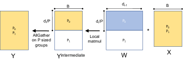
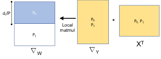
Communication costs of pure model parallelism. In the model parallel case, the computation of the loss in the forward pass can be computed by distributing the model parameters $W$ as shown in Fig. 1.

Figure 3. Illustration of domain parallel approach for $P=4$. For NCHW format, it is best to distribute along the height to avoid non-contiguous memory accesses. NCHW format corresponds to the data layout in the memory, where the data runs fastest in width, height, channel size, and then across batch size.

Consider a convolutional layer without loss of generality: each process performs a subset of the convolutions on the input activations and computes a subset of the output activations. For instance, assume one of the layers consists of $Y_{C}$ $k_{h}\times k_{w}\times X_{C}$ convolutions, where $k_{h},\ k_{w}$ is the size of each convolution filter and $X_{C},\ Y_{C}$ are the sizes of input and output channels. In the model parallel case, the kernels are distributed so that each process gets $Y_{C}/P$ filters and computes the corresponding $Y_{C}/P$ channels of the output activation. As computations of the other layers would require access to all of the previous activations, one needs to perform an all-gather operation per layer. Backpropagation also requires an all-reduce communication during $\Delta_{X}$ calculation (details are discussed in appendix). This yields the following communication complexity for the model parallel case:

(3) $$\begin{split}T_{\mathit{comm}}(\mathit{model})&=\sum_{i=1}^{L}\left(\alpha\lceil\log(P)\rceil+\beta B\frac{P-1}{P}d_{i}\right)\\ &+2\sum_{i=2}^{L}\left(\alpha\lceil\log(P)\rceil+\beta B\frac{P-1}{P}d_{i-1}\right),\end{split}$$

where $P$ is the number of processes, $L$ is the number of DNN layers, $\alpha$ is the network latency, and $\beta$ is the inverse bandwidth. The first sum considers the cost for all-gather required after every layer, and the second sum considers the all-reduce cost for backpropagating activation gradients. Note that the second sum starts from $i=2$ as we do not need to backpropagate the gradient beyond the first layer. This analysis assumes the use of Bruck’s algorithm for all-gather and ring algorithm for all-reduce (thakur2005optimization, ). We note that the complexity depends on the mini-batch size. The model parallel approach was partially used in AlexNet (krizhevsky2012imagenet, ), where the model was split into two GPUs. The original GoogLeNet work also exploited a certain amount of model parallelism (szegedy2015going, ). Distributed DNN training engines that rely solely on model parallelism also exist (coates2013deep, ), especially for low-latency high-bandwidth systems.

The other possibility for distributing the SGD computation is data parallelism. This can be performed either by distributing the data over the batch size, or partition each individual image. We refer to the latter as domain parallelism, which will be discussed further below.

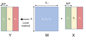
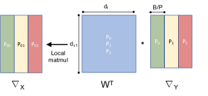
Communication costs of pure batch parallelism. For the batch parallel case, the reduction for the gradient computation over the mini-batch sum (1) can be computed independently by each process. This approach is known as batch parallel method, where each process computes a partial sum, followed by an all-reduce to compute the mini-batch gradient. This communication cost is due to the reduction that is needed to form $\Delta_{W}=\Delta_{Y}X^{T}$ product. The communication complexity for the batch parallel approach using ring algorithm for all-reduce (thakur2005optimization, ) is:

(4) $$T_{\mathit{comm}}(\mathit{batch})=2\sum_{i=0}^{L}\left(\alpha\lceil\log(P)\rceil+\beta\frac{P-1}{P}\lvert W_{i}\rvert\right),$$

where $|W_{i}|$ is the total number of model parameters in the $i$th layer. Here, the factor of 2 is merely due to the all-reduce algorithm (thakur2005optimization, ). Note that for $P\gg 1$ the bandwidth costs are independent of $P$ and unlike the model parallel case does not depend on the batch size. Most of the current work on distributed training uses batch parallel to scale training (goyal2017accurate, ; you2017imagenet, ). The DistBelief paper (dean2012large, ) provides easy-to-understand descriptions of model and batch parallelism.

For a convolutional layer, based on Equation 2, the ratio of communication volume between pure model and batch parallelism becomes

$$\frac{T_{\mathit{comm-volume}}(\mathit{batch})}{T_{\mathit{comm-volume}}(\mathit{model})} =\frac{2\lvert W_{i}\rvert}{3Bd_{i}}=\frac{(2k_{h}k_{w}X^{i}_{C})Y^{i}_{C}}{3BY^{i}_{H}Y^{i}_{W}Y^{i}_{C}}$$

(5) $$=\frac{2k_{h}k_{w}X^{i}_{C}}{3BY^{i}_{H}Y^{i}_{W}}$$

Consequently, whenever $B>(2k_{h}k_{w}X^{i}_{C}/3Y^{i}_{H}Y^{i}_{W})$, pure batch parallelism is favorable to pure model parallelism. Surprisingly, it is not a foregone conclusion that batch parallelism is always favorable to model parallelism for convolutional layers. For several convolutional layers that are used in practice (such as those found in AlexNet with 3x3 filters on 13x13x384 activations), model parallelism has lower communication volume than batch parallelism for $B\leq 12$.

If one were to switch from a data parallel distribution shown in Figure 2 to a model parallel distribution shown in Figure 1, the only added communication cost is the redistribution of $X$ to processes using an all-gather operation, with an associated cost of

(6) $$T_{\mathit{comm}}(\text{redistribute batch to model})=\alpha\lceil\log(P)\rceil+\beta B\frac{P-1}{P}d_{i}.$$

It is important to note that this redistribution cost is asymptotically free because the subsequent model parallel step has communication cost that is three times of the cost of the redistribution.

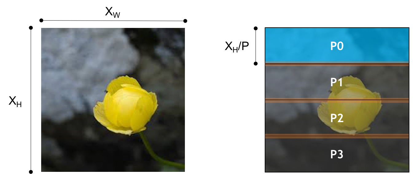
Communication costs of pure domain parallelism. A third possibility for parallelization is domain parallel (jin2018spatially, ), where one can decompose the input activation map as shown in Fig. 3. Here each process contains all of the model parameters (as in the pure batch parallel case), but performs the convolutions only on a subset of the input image, and writes a subset of the output activations. For convolutions with filter size larger than one, we have to perform a halo exchange to communicate the boundary points. This can be performed as a non-blocking, pair-wise exchange while the convolution is being applied to the rest of the image. This means that the convolutions that do not require this boundary data could be computed while the communication is being performed. The cost of the communication in this case will be:

(7) $$\begin{split}T_{\mathit{comm}}(\mathit{domain})=&\sum_{i=0}^{L}\left(\alpha+\beta BX^{i}_{W}X^{i}_{C}\lfloor k^{i}_{h}/2\rfloor\right)\\ +&\sum_{i=0}^{L}\left(\alpha+\beta BY^{i}_{W}Y^{i}_{C}\lfloor k^{i}_{w}/2\rfloor\right)\\ +2&\sum_{i=0}^{L}\left(\alpha\lceil\log(P)\rceil+\beta\frac{P-1}{P}|W_{i}|\right),\end{split}$$

where $X^{i}_{W},\ X^{i}_{H},\ X^{i}_{C},Y^{i}_{W},\ Y^{i}_{H},\ Y^{i}_{C}$ are the input/output activation’s width, height, and channel size in the $i$th layer, and $k^{i}_{h},\ k^{i}_{w}$ is the corresponding convolution size of that layer. Note that for a $1\times 1$ convolution no communication is needed. For layers with large input activation size and large number of convolution filters, this approach can reduce the computation time with good strong scaling efficiency. However, it is not effective for small image sizes and not applicable to fully connected layers.

Model parallelism, as published in literature, corresponds to performing a 1D distribution of the matrix $W_{i}$, replicating $X_{i}$ and gathering $Y_{i}$ multivectors after multiplication. The $k$th processor can perform its local matrix multiplication of the form $W_{i}(k,:)\,X_{i}$ without any communication, but in order to fully assemble $Y_{i}$, each processor needs to gather other components from other processes. Even if input/output multivectors were also distributed, the communication bounds stay the same, because while this communication time would not be necessary for the output $Y_{i}$, it would be needed for gathering $X_{i}$ before the local multiplication.

By contrast, in data parallelism, every process starts with the same parameters, which get updated by the same gradient. In fact, the forward pass of batch parallel training needs no communication. The communication in this case happens during backpropagation, where a collective all-reduce operation is needed to compute the total sum of the partial gradients. The parallel matrix multiplications in the batch parallel case are illustrated in Figure 2, where the input activations $X_{i}$ and the output activations $Y_{i}$ are distributed 1D columnwise to processes.

2.3. Integrated Model and Batch Parallelism

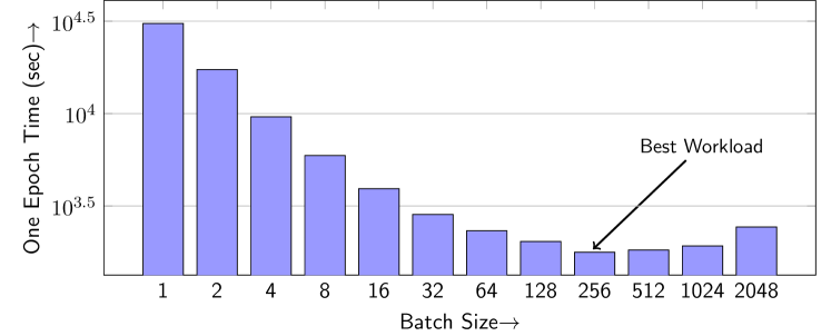
We first discuss the integrated model and batch parallelism and then discuss the full integration with domain parallelism which extends the scalability limit of the pure batch method. Batch parallelism has a favorable communication complexity, but there is an inherent limit on increasing the batch size. Furthermore, small batch size training is not efficient in terms of hardware utilization and ultimately training time. This is due to the fact that small matrix-matrix operations (aka level-3 BLAS operations) cannot use all the hardware resources, in terms of cores or vectorized units. This is empirically shown in Fig. 4, where we report one epoch training time of AlexNet for different batch sizes measured on a single Intel Knights Landing (KNL) processor. The fastest training time is achieved with a batch size of $256$. With the batch parallel approach one has no choice but to reduce per process batch size for scaling before hitting the limit of 1 batch per process.

Figure 4. One epoch training time of AlexNet computed on a single KNL. Increasing batch size up to 256, reduces the time due to better use of hardware resources and fewer SGD updates.

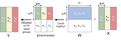
Our integrated batch and model parallel approach allows us to reduce the communication overhead of the pure batch parallel case. Here, we consider replicating a subset of $W_{i}$ as opposed to all of it, a concept that has been explored under the name of 1.5D algorithms for matrix multiplication (spdmmm16, ). We think of our process grid logically partitioned as $P=P_{r}\times P_{c}$. Each process holds $(1/P_{r})$th piece of $W_{i}$, effectively replicating $W_{i}$ matrix $P_{c}$ times (as opposed to $P$ times in batch parallelism). Conversely, data matrices are replicated $P_{r}$ times and each process holds $(1/P_{c})$th piece of $X_{i}$ and $Y_{i}$. Communication cost of this 1.5D algorithm, which is illustrated in Figure 5, is:

(8) $$\begin{split}T_{comm}=&\sum_{i=1}^{L}\left(\alpha\lceil\log(P_{r})\rceil+\beta\frac{B}{P_{c}}\frac{P_{r}-1}{P_{r}}{d_{i}}\right)\\ +&2\sum_{i=2}^{L}\left(\alpha\lceil\log(P_{r})\rceil+\beta\frac{B}{P_{c}}\frac{P_{r}-1}{P_{r}}{d_{i-1}}\right)\\ +&2\sum_{i=0}^{L}\left(\alpha\lceil\log(P_{c})\rceil+\beta\frac{P_{c}-1}{P_{c}}\frac{|W_{i}|}{P_{r}}\right).\end{split}$$

Note that unlike in Eq. 4, the all-reduce communication volume is now reduced by a factor of $P_{r}$. This provides a theoretically sound integration of batch and model parallelism. It can be especially valuable for networks with many fully connected layers. Furthermore, this algorithm automatically selects the best configuration to distribute the model and batch parallel work given a fixed batch size on $P$ processes. The closest approach to ours is the hybrid model/batch parallel approach described by Das et al. (das2016distributed, ), but that paper does not describe the details of the partitioning of the data and the model to the processes. In addition, the authors claim that using any other dimension to extract parallelism would always be sub-optimal, which we show not be true in general by using domain parallelism.

Similar to the analysis of pure model and pure batch cases, the cost of redistribution is asymptotically amortized in this integrated batch and model parallel case as well. In particular, if one were to switch process grids in between layers, say from a pure batch case ($1\times P$ grid) to a balanced case ($\sqrt{p}\times\sqrt{p}$) grid, the communication costs would asymptotically stay constant.

For the curious reader familiar with the theory of parallel matrix multiplication, we would like to clarify why we consider our approach a 1.5D algorithm, as opposed to a 2D algorithm such as Cannon’s algorithm (cannon, ) or SUMMA (van1997summa, ). 2D matrix multiplication algorithms are optimal in terms of their memory usage; that is, each processor only holds $(1/p)$th of the total memory needed to store all three matrices (2 inputs and 1 output). In other words, there is no replication. The class of .5D algorithms (of which 1.5D algorithm is a member), by contrast, are not optimal in terms of memory consumption. At least one matrix is replicated multiple times, which often results in an asymptotic reduction in communication costs (ballard2011minimizing, ). This is indeed the case for the algorithm described in Figure 5.

Figure 5. 1.5D matrix multiply illustration for integrated parallel DNN training (top: forward pass, middle/bottom: weight gradient computation) using a $2\times 3$ process grid indexed as $P_{ij}$.

Figure 6. Strong scaling analysis of integrated model and batch parallel approach using the simulated results. The orange bar shows the total communication time, with the cross hatched portion representing the time spent in batch parallel communication (i.e. the ring all-reduce during backprop). Here we use the same process grid for all layers, which means some amount of model parallelism is used for both convolutional and FC layers when $P_{r}>1$. The speedup for the total time compared to pure batch parallel is shown in bold text on top of the best bar chart. We also report the corresponding speedup for communication time in parenthesis. In strong scaling, we keep the global batch size fixed, and increase the number of processes to reduce the training time.

2.4. Integrated Model, Batch and Domain Parallelism

The pure batch parallel method has a theoretical strong scaling limit of $B$. In the limit each process gets a batch size of one (i.e. it reads a single data). It is possible to extend this limit with the integrated model and batch parallel approach discussed above. But this approach is sub-optimal for early layers of the network, as the all-gather communication volume is very high there (Eq. 8). This is due to the fact that this communication volume depends on the size of the activation map (i.e. $Y_{i}$) which is prohibitively large in the beginning layers.

Figure 7. Strong scaling analysis of integrated model and batch parallel approach using the simulated results. Model parallelism is used in FC layers only. Notice the significant improvement in best time compared to Fig. 6 which uses model parallelism in both convolutional and FC layers.

However, as we show below the domain parallel approach has a favorable communication complexity for early layers of a neural network where the input activation size is large. For these layers it is favorable to use domain parallelism instead of model parallelism, as it leads to a smaller communication volume that can actually be overlapped with part of the computation in both forward and backward pass. Note that in model parallel one has to perform a blocking all-gather operation which is detrimental for performance. Moreover, the domain parallel approach does not require any communication for $1\times 1$ convolutions which are actually becoming a dominant portion of the network in recent architectures (he2016deep, ). However, for fully connected layers the halo exchange region will consist of all of the input activations. To avoid that large communication cost we can actually integrate all the three parallelism methods. The communication complexity for integrating all the three methods would then become:

(9) $$\begin{split}T_{comm}=&\sum_{i\in L_{M}}\left(\alpha\lceil\log(P_{r})\rceil+\beta\frac{B}{P_{c}}\frac{P_{r}-1}{P_{r}}{d_{i}}\right)+\\ 2&\sum_{i\in L_{M}}\left(\alpha\lceil\log(P_{r})\rceil+\beta\frac{B}{P_{c}}\frac{P_{r}-1}{P_{r}}{d_{i-1}}\right)+\\ 2&\sum_{i\in L_{M}}\left(\alpha\lceil\log(P_{c})\rceil+\beta\frac{P_{c}-1}{P_{c}}\frac{|W_{i}|}{P_{r}}\right)+\\ &\sum_{i\in L_{D}}\left(\alpha+\beta\frac{B}{P_{c}}X^{i}_{W}X^{i}_{C}\lfloor k^{i}_{h}/2\rfloor\right)+\\ &\sum_{i\in L_{D}}\left(\alpha+\beta\frac{B}{P_{c}}X^{i+1}_{W}X^{i+1}_{C}\lfloor k^{i}_{w}/2\rfloor\right)+\\ 2&\sum_{i\in L_{D}}\left(\alpha\lceil\log(P)\rceil+\beta\frac{P-1}{P}{|W_{i}|}\right),\end{split}$$

where $L_{M}$ and $L_{D}$ refer to the list of layers where the $P_{r}$ groups are used to partition either the model or the domain. Note that for $L_{M}=L$, $L_{D}=0$, we get the integrated model and batch parallel complexity as expected.

The choice of whether to partition the model or the domain can be made by computing the communication complexity. Generally, it is better to use domain parallelism for the initial layers of the network, since the activation size is large. However, the domain parallel approach loses its communication advantage for fully connected layers (for which $k_{h}=X_{H},\ k_{w}=X_{W}$).

3. Simulated Performance in Training AlexNet

Simulation setup. We analytically explore the spectrum of both the integrated batch and model parallel approach, as well as the full integration with domain parallelism by simulating Eq. 8 and Eq. 9. To limit the number of variables, we fix a network (AlexNet), a training set of images (ImageNet LSVRC-2012 contest), and a computing platform (NERSC’s Cori supercomputer). These fixed options, described in Table 1, are chosen just to develop a proof-of-concept of our integrated batch and model parallel approach.

We considered two scenarios: (a) $B\geq P$: here the relevant integration is between model and batch parallel approaches and domain parallelism is not used as its communication overhead is higher than batch parallel (Eq. 7) (b) $B<P$: This is the case where we reach the maximum scaling limit of the batch parallel method, and use domain parallelism to scale beyond this (Eq. 9). For the first scenario, we considered two cases. At first, the same process grid is used for all layers of the network, which means that if $P_{r}>1$ then some amount of model parallelism will be used even in convolutional layers. Then we considered the improved case where we force $P_{r}=1,P_{c}=P$ for the convolutional layers and use varying $P_{r}\times P_{c}$ grids for the fully connected layers.

We compute the communication time for a single iteration with various choices of the mini-batch size $B$, the number of processes, and the configuration of process grid $P_{r}\times P_{c}$. Using this data, we then compute the communication time for a complete epoch by multiplying the communication time form Eq. 4 by $N/B$. A typical simulation of the Neural Network would require many epochs of training (100 epochs in the case of AlexNet (krizhevsky2012imagenet, )).

Furthermore, we also consider the computational time by empirically measuring the time needed for an SGD iteration for AlexNet on a single KNL using Intel Caffe as shown in Fig. 4. We use this data for cases with the same computational workload to compute the total run time.

	Fixed options	Relevant parameters
Network	AlexNet (krizhevsky2012imagenet, )	5 convolutional and
architecture	parameters: 61M	3 fully connected layers
Training	ImageNet	training images: 1.2M
images	LSVRC-2012 contest	Number of categories: 1000
Computing	NERSC’s Cori2	Processor: Intel KNL
platform		latency: $\alpha=2\mu$ s
		inverse bw: $1/\beta=6$GB/s

Table 1. Fixed parameters used to simulate the cost of training neural networks using integrated batch and model parallel approach. We only change the mini-batch size and the number and configurations of processes in the presented results.

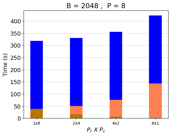
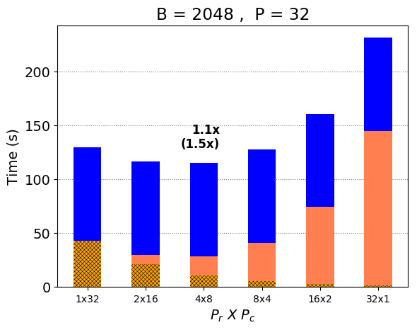
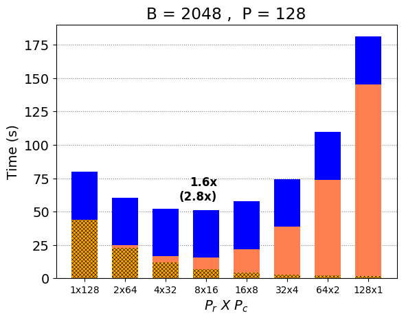
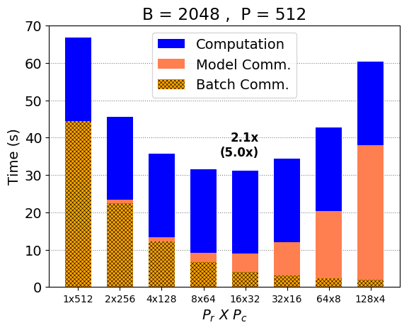
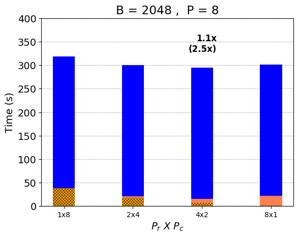
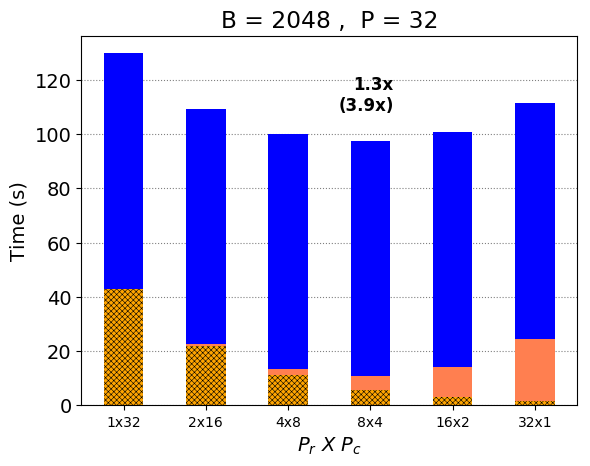
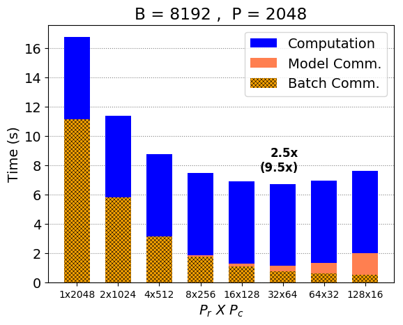
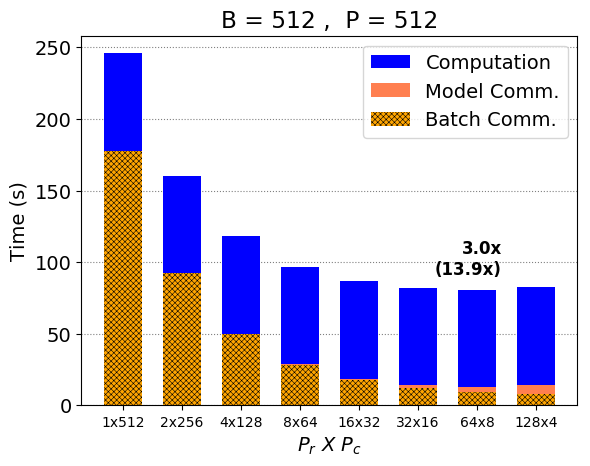
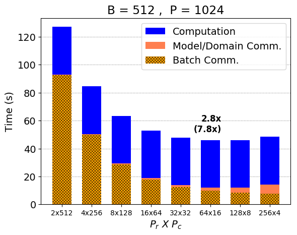
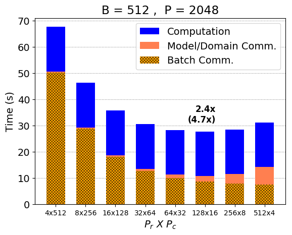
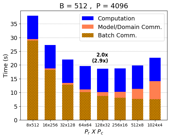
Strong scaling with a fixed mini-batch size. At first, we present the strong scaling results for integrated model and batch. We initially apply the integrated method in a way that the same process grid is used for all layers of the network, which means that if $P_{r}>1$ then some amount of model parallelism will be used even in convolutional layers. The results are shown Fig. 6 where the training was performed using $P=8$ to $P=512$ processes with a fixed mini-batch size of $B=2,048$. In each subfigure in Fig. 6, only the configurations of the process grid vary. We can see that even in the naive format, better performance can be attained with an integrated batch and model parallelism, especially for larger values of $P$. For example, on $P=512$ processes, the best performance is observed with $16\times 32$ process grid which results in $2.1\times$ speed up in the overall runtime and $5.0\times$ speedup in communication ( Figure 6-d). The improved performance is primarily driven by reduced communication needed by the integrated model and batch parallel approach (notice the reduction of the communication volume of the parameters by $P_{r}$ factor in Eq. 8). However, the benefit of the integrated approach is not realized on a relatively small number processors, such as with 8 processes in Figure 6(a). The first reason is that here the main bottleneck is computation. Moreover, the communication time for model parallel does not scale down since per process batch size is very large (note the $B/P_{c}$ term in Eq.8).

Next, we considered the improved case where we force $P_{r}=1,P_{c}=P$ for the convolutional layers and use varying $P_{r}\times P_{c}$ grids for the fully connected layers. For the configurations considered, this results in using pure batch parallelism in convolutional layers and both model and batch parallelism in FC layers as shown in Figure 7. Making the convolutional layer pure batch parallel can reduce the communication significantly, as evident by comparing Fig. 7 and Fig. 6. For instance, the case with $B=2048,\ P=512$ results in $2.5\times$ speedup in overall runtime and $9.7\times$ speedup in communication time (Figure 7-d). We also show how the results would change if we consider a perfect overlap between communication and computation as shown in Fig. 8. This overlapping can only be performed with the backpropagation phase, where the all-reduce communication can happen while the transpose convolution of next layers are being performed (which accounts for two-thirds of the communication). Even in this setting there is $2.0\times$ speedup. We believe that this speed up is actually going to increase, given the new domain specific architectures optimized for accelerating the computation part of neural network training/inference.

Figure 8. Here we show results for perfect overlapping of communication with backpropagation part of the computations.

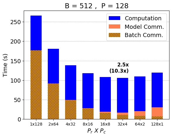
Scaling with a variable mini-batch size. We now consider weak scaling by varying the mini-batch size and the process grid simultaneously, as shown in Fig. 9. Here we use choose model/batch parallel based on the complexity analysis of Eq. 8 (similar to the strong scaling shown in Fig. 7). In each subfigure, only the configurations of the process grid vary for a fixed $P$ and $B$. Similar to the strong scaling results, we observe that the integrated approach can reduce the communication significantly as we change the mini-batch size.

Figure 9. Simulated cost of integrated model and batch parallel method. We present weak scaling results for the communication and computation complexity when training AlexNet. The speedup for the total time compared to pure batch parallel is shown in bold text on top of the best bar chart. We also report the corresponding speedup for communication time in parenthesis. Here we use the same process grid for all layers, which results in using some amount of model parallelism (when $P_{r}>1$) for convolutional layers as well, which is sub-optimal. A better approach is to use pure batch parallelism for convolutional layers.

Figure 10. Illustration of how domain parallel can extend strong scaling limit of pure batch parallelism.

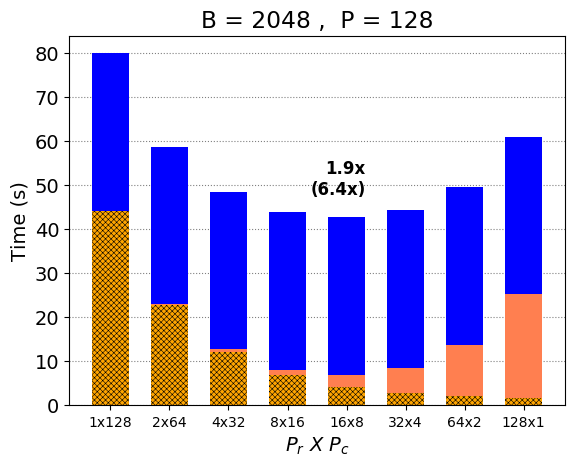
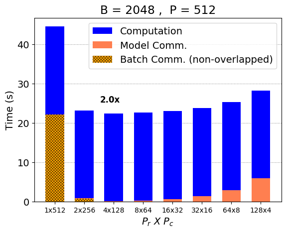
Scaling beyond batch size. The pure batch parallel method has a scaling limit to the maximum batch size that one can use. However, one cannot increase batch size indefinitely as it is known to be detrimental to the performance of the Neural Network (keskar2016large, ). Recent works have tried to increase this limit by changing the hyper-parameters of SGD (goyal2017accurate, ; you2017scaling, ), but these methods also hit a limit and have been only shown to work for certain applications in ImageNet classification. So a natural question is how do we scale beyond this theoretical limit with pure batch parallelism? One could use the integrated approach and scale the model part for all layers, but as shown above this results in sub-optimal communication time. A better approach is to use an integrated batch, domain, and model parallel where for the initial layers we use domain parallel instead of the model. Note that the domain parallel approach requires a much smaller communication as compared to model parallel, and actually requires no communication for $1\times 1$ convolutions (Eq. 7). To illustrate this, we show the scaling results for $B=512$ up to $P=4096$ in Fig. 10. In Fig. 10(a), convolutional layers use pure batch parallelism with per-process batch size set to one. By contrast, in Fig. 10(c-d), each image is partitioned into 2,4, and 8 parts where each process works with one part of the image. Using this integrated batch, domain, and model parallel approach, we can continue scaling beyond the theoretical limit with pure batch parallelism (beyond 512 processes in Fig. 10).

4. Discussion

One disadvantage of batch parallelism over model and domain parallelism is that it tends to change the convergence characteristics of DNN training algorithms as larger minibatches beyond a certain point can hurt accuracy. Our integrated framework also provides guidance on how to choose the right parallelization parameters if the user decides to limit the maximum allowable batch parallelism in light of accuracy concerns related to large batch sizes.

Due to DNN training being computational intensive, memory considerations have been secondary to performance. Solutions that exploit pure data parallelism often replicate the whole model in each node. By contrast, the 1.5D matrix-multiplication algorithms used by our integrated parallel approach cut down the model replication cost by a factor of $p_{r}$, at the cost of an increase in data replication by a factor of $p_{c}$. Like our communication costs, our memory costs are simply a linear combination of the memory costs of these two extremes of pure data and pure model parallelism.

We also considered the alternative of using 2D matrix multiplication algorithms instead of the 1.5D algorithm. The popular stationary-C variant of the 2D SUMMA algorithm (van1997summa, ) is symmetrical in nature; in the sense that it communicates equal proportions of both input matrices for an operation $C=AB$. When matrices $A$ and $B$ are of comparable sizes, this is a good fit. Often in deep learning, one of the matrices is bigger than the other. For such situations, there are other less-common variants of SUMMA that keep another matrix stationary (schatz2016parallel, ). These algorithms are more complicated that our 1.5D algorithm, and communicate more data either asymptotically or by higher constants.

Consider stationary-A SUMMA, which is the best fit for the forward propagation $Y=WX$ among all 2D algorithm variants. This algorithm has $4$ communication steps compared to a single step in our algorithm. For simplicity assume that $d_{i}=d_{i-1}$. Also assume that $p_{r}$ and $p_{c}$ are large enough such that $(p_{r}-1)/p_{r}\approx(p_{c}-1)/p_{c}\approx 1$. When $\lvert W_{i}\rvert>Bd_{i}$, it communicates $2B\,d_{i}/p_{r}+B\,d_{i}/p_{c}$ words, compared to our 1.5D algorithm’s $B\,d_{i}/p_{c}$ words. In that sense, its communication costs approach 1.5D when $p_{r}\gg p_{c}$ but never surpass it. When $\lvert W_{i}\rvert<Bd_{i}$, all possible 2D algorithms become asymptotically slower because they have to communicate two matrices and no matter which two they choose, the costs become higher than solely communicating the single smaller matrix. By contrast, our 1.5D algorithm communicates only that single matrix. Hence, there is no regime where 2D becomes strictly favorable in terms of communication volume. The main advantage of 2D algorithms over 1.5D algorithm is that their memory consumption is optimal in the sense that they do not perform any asymptotic data replication. Memory consumption optimality might be a legitimate concern depending on the platform and the DNN model size.

5. Conclusion

We presented an integrated parallel algorithm that exploits model, batch, and domain parallelism in training deep neural networks (DNNs). We discussed the associated communication complexity by analyzing both forward and backwards pass, and showed that theoretically the integrated parallel approach can achieve better run time. Furthermore, the integrated parallel approach increases the scalability limit of the pure batch parallel method that is commonly used, by decomposing both along the weight matrix as well as the domain. This approach allows optimal selection of per process batch size and model size which results in better throughput as compared to pure batch/model parallel algorithms.

Our analysis toolset is primarily comprised of parallel matrix algorithms. In particular, the analysis of our integrated model and batch parallel approach relies on a communication-avoiding 1.5D matrix multiplication algorithm. This explicit connection between parallel matrix algorithms and DNN training has the potential to enable the discovery of new classes of parallel algorithms and lower bounds for training DNNs.

6. Acknowlegments

This manuscript has been authored by an author at Lawrence Berkeley National Laboratory under Contract No. DE-AC02-05CH11231 with the U.S. Department of Energy. The U.S. Government retains, and the publisher, by accepting the article for publication, acknowledges, that the U.S. Government retains a non-exclusive, paid-up, irrevocable, world-wide license to publish or reproduce the published form of this manuscript, or allow others to do so, for U.S. Government purposes.

This work was supported by the Laboratory Directed Research and Development Program of Lawrence Berkeley National Laboratory under U.S. Department of Energy Contract No. DE-AC02-05CH11231.

The authors would also like to acknowledge generous support from Intel’s VLAB team for providing access to KNLs.

7. Appendix: Detailed Derivations

7.1. Detailed Derivation of the Forward Pass

During the forward pass for data parallel, each process reads a mini-batch size of $B/P$ input images and the calculations are performed as follows:

$$Y_{i}=WX_{i},$$

where $X_{i}$ and $Y_{i}$ is the $i$th column of X and Y, respectively. Here, $W$ is shared and no communication is needed. However, in the model parallel case we have:

$$Y_{p,i}=W_{p}X_{i},$$

where $p$ denotes the process id, $W_{p}$ is the fraction of weights in each process, and $Y_{p,i}$ is the fraction of output activation computed locally. This local component needs to be communicated via an all-gather operation to concatenate all partial activations for the next layer’s computation.

7.2. Detailed Derivation of Backpropagation

During backpropagation, the gradient of the loss functional with respect to output activations $Y$ is given ($\Delta_{Y}=\frac{\mathop{}\!\mathrm{d}\mathcal{J}}{\mathop{}\!\mathrm{d}Y}$), and one has to compute the gradient with respect to the weights ($\Delta_{W})$ as well as the input feature map ($\Delta_{X})$. The latter is needed for propagating the gradient to lower layers. We use capital letters for input and output activation as we are mostly interested in the mini-batch setting $B>1$. Using chain rule we have:

$$\Delta_{W}=\frac{\mathop{}\!\mathrm{d}\mathcal{J}}{\mathop{}\!\mathrm{d}W}=\sum_{i=1}^{B}\frac{\mathop{}\!\mathrm{d}\mathcal{J}}{\mathop{}\!\mathrm{d}Y_{i}}\frac{\mathop{}\!\mathrm{d}Y_{i}}{\mathop{}\!\mathrm{d}W}=\sum_{i=1}^{B}\frac{\mathop{}\!\mathrm{d}\mathcal{J}}{\mathop{}\!\mathrm{d}Y_{i}}X_{i}^{T}=\Delta_{Y}X^{T},$$

Now in the distributed case, we have:

$$\frac{\mathop{}\!\mathrm{d}\mathcal{J}}{\mathop{}\!\mathrm{d}W}^{p}=\sum_{i=1}^{B/P_{c}}\frac{\mathop{}\!\mathrm{d}\mathcal{J}}{\mathop{}\!\mathrm{d}Y_{i}}X_{i}^{T},$$

$$\frac{\mathop{}\!\mathrm{d}\mathcal{J}}{\mathop{}\!\mathrm{d}W}=\sum_{k=1}^{P_{c}}\frac{\mathop{}\!\mathrm{d}\mathcal{J}}{\mathop{}\!\mathrm{d}W}^{p}.$$

where $p$ is the process id. Notice that the last step requires an all-reduce between $P_{c}$ processes, but no communication is needed for the model parallel part as the input activation is already communicated via the all-gather collective of forward pass. To backpropagate the gradient, one needs to compute $\Delta_{X}=\frac{\mathop{}\!\mathrm{d}\mathcal{J}}{\mathop{}\!\mathrm{d}X}$ as well. We derive it for one column of $\Delta_{X}$ below as each column can be computed independently:

$$\Delta_{X_{i}}=\frac{\mathop{}\!\mathrm{d}\mathcal{J}}{\mathop{}\!\mathrm{d}X_{i}}=\frac{\mathop{}\!\mathrm{d}\mathcal{J}}{\mathop{}\!\mathrm{d}Y_{i}}\frac{\mathop{}\!\mathrm{d}Y_{i}}{\mathop{}\!\mathrm{d}X_{i}}=W^{T}\frac{\mathop{}\!\mathrm{d}\mathcal{J}}{\mathop{}\!\mathrm{d}Y_{i}}=W^{T}\Delta_{Y_{i}},$$

Here in the distributed model parallel part, the weight matrix is distributed among $P_{r}$ processes. To backpropagate the gradient, every process computes its contribution to the gradient followed by an all-reduce collective between $P_{r}$ processes:

$$\frac{\mathop{}\!\mathrm{d}\mathcal{J}}{\mathop{}\!\mathrm{d}X_{i}}^{p}=W^{T}\frac{\mathop{}\!\mathrm{d}\mathcal{J}}{\mathop{}\!\mathrm{d}Y_{i}},$$

$$\frac{\mathop{}\!\mathrm{d}\mathcal{J}}{\mathop{}\!\mathrm{d}X_{i}}=\sum_{k=1}^{P_{r}}\frac{\mathop{}\!\mathrm{d}\mathcal{J}}{\mathop{}\!\mathrm{d}X_{i}}^{k}.$$

References

- [1] Grey Ballard, James Demmel, Olga Holtz, and Oded Schwartz. Minimizing communication in numerical linear algebra. SIAM Journal on Matrix Analysis and Applications, 32(3):866–901, 2011.
- [2] Lynn Elliot Cannon. A cellular computer to implement the Kalman filter algorithm. PhD thesis, Montana State University, 1969.
- [3] Ernie Chan, Marcel Heimlich, Avi Purkayastha, and Robert Van De Geijn. Collective communication: theory, practice, and experience. Concurrency and Computation: Practice and Experience, 19(13):1749–1783, 2007.
- [4] Trishul M Chilimbi, Yutaka Suzue, Johnson Apacible, and Karthik Kalyanaraman. Project adam: Building an efficient and scalable deep learning training system. In OSDI, volume 14, pages 571–582, 2014.
- [5] Adam Coates, Brody Huval, Tao Wang, David Wu, Bryan Catanzaro, and Ng Andrew. Deep learning with COTS HPC systems. In International Conference on Machine Learning, pages 1337–1345, 2013.
- [6] Dipankar Das, Sasikanth Avancha, Dheevatsa Mudigere, Karthikeyan Vaidynathan, Srinivas Sridharan, Dhiraj Kalamkar, Bharat Kaul, and Pradeep Dubey. Distributed deep learning using synchronous stochastic gradient descent. arXiv preprint arXiv:1602.06709, 2016.
- [7] Jeffrey Dean, Greg Corrado, Rajat Monga, Kai Chen, Matthieu Devin, Mark Mao, Andrew Senior, Paul Tucker, Ke Yang, Quoc V Le, et al. Large scale distributed deep networks. In Advances in neural information processing systems, pages 1223–1231, 2012.
- [8] Priya Goyal, Piotr Dollár, Ross Girshick, Pieter Noordhuis, Lukasz Wesolowski, Aapo Kyrola, Andrew Tulloch, Yangqing Jia, and Kaiming He. Accurate, large minibatch SGD: Training ImageNet in 1 hour. arXiv preprint arXiv:1706.02677, 2017.
- [9] Mohammad Havaei, Axel Davy, David Warde-Farley, Antoine Biard, Aaron Courville, Yoshua Bengio, Chris Pal, Pierre-Marc Jodoin, and Hugo Larochelle. Brain tumor segmentation with deep neural networks. Medical image analysis, 35:18–31, 2017.
- [10] Kaiming He, Xiangyu Zhang, Shaoqing Ren, and Jian Sun. Deep residual learning for image recognition. In Proceedings of the IEEE conference on computer vision and pattern recognition, pages 770–778, 2016.
- [11] Peter Jin, Boris Ginsburg, and Kurt Keutzer. Spatially parallel convolutions. ICLR 2018 Workshop, 2018.
- [12] Peter H Jin, Qiaochu Yuan, Forrest Iandola, and Kurt Keutzer. How to scale distributed deep learning? arXiv preprint arXiv:1611.04581, 2016.
- [13] Nitish Shirish Keskar, Dheevatsa Mudigere, Jorge Nocedal, Mikhail Smelyanskiy, and Ping Tak Peter Tang. On large-batch training for deep learning: Generalization gap and sharp minima. arXiv preprint arXiv:1609.04836, 2016.
- [14] Jiwon Kim, Jung Kwon Lee, and Kyoung Mu Lee. Accurate image super-resolution using very deep convolutional networks. In Proceedings of the IEEE Conference on Computer Vision and Pattern Recognition, pages 1646–1654, 2016.
- [15] Penporn Koanantakool, Ariful Azad, Aydın Buluç, Dmitriy Morozov, Sang-Yun Oh, Leonid Oliker, and Katherine Yelick. Communication-avoiding parallel sparse-dense matrix-matrix multiplication. In Proceedings of the IPDPS, 2016.
- [16] Alex Krizhevsky, Ilya Sutskever, and Geoffrey E Hinton. Imagenet classification with deep convolutional neural networks. In Advances in neural information processing systems, pages 1097–1105, 2012.
- [17] Jonathan Long, Evan Shelhamer, and Trevor Darrell. Fully convolutional networks for semantic segmentation. In Proceedings of the IEEE Conference on Computer Vision and Pattern Recognition, pages 3431–3440, 2015.
- [18] A. Mang, S. Tharakan A. Gholami, N. Himthani, S. Subramanian, J. Levitt, M. Azmat, K. Scheufele, M. Mehl, C. Davatzikos, B. Barth, and G. Biros. SIBIA-GlS: Scalable biophysics-based image analysis for glioma segmentation. The multimodal brain tumor image segmentation benchmark (BRATS), MICCAI, 2017.
- [19] Benjamin Recht, Christopher Re, Stephen Wright, and Feng Niu. Hogwild: A lock-free approach to parallelizing stochastic gradient descent. In Advances in neural information processing systems, pages 693–701, 2011.
- [20] Shaoqing Ren, Kaiming He, Ross Girshick, and Jian Sun. Faster R-CNN: Towards real-time object detection with region proposal networks. In Advances in neural information processing systems, pages 91–99, 2015.
- [21] RO Rogers and David B Skillicorn. Using the BSP cost model to optimise parallel neural network training. Future Generation Computer Systems, 14(5):409–424, 1998.
- [22] Martin D Schatz, Robert A Van de Geijn, and Jack Poulson. Parallel matrix multiplication: A systematic journey. SIAM Journal on Scientific Computing, 38(6):C748–C781, 2016.
- [23] Christian Szegedy, Wei Liu, Yangqing Jia, Pierre Sermanet, Scott Reed, Dragomir Anguelov, Dumitru Erhan, Vincent Vanhoucke, and Andrew Rabinovich. Going deeper with convolutions. In Proceedings of the IEEE conference on computer vision and pattern recognition, pages 1–9, 2015.
- [24] Rajeev Thakur, Rolf Rabenseifner, and William Gropp. Optimization of collective communication operations in MPICH. The International Journal of High Performance Computing Applications, 19(1):49–66, 2005.
- [25] Robert A Van De Geijn and Jerrell Watts. SUMMA: Scalable universal matrix multiplication algorithm. Concurrency-Practice and Experience, 9(4):255–274, 1997.
- [26] Bichen Wu, Forrest Iandola, Peter H Jin, and Kurt Keutzer. Squeezedet: Unified, small, low power fully convolutional neural networks for real-time object detection for autonomous driving. arXiv preprint arXiv:1612.01051, 2016.
- [27] Bichen Wu, Alvin Wan, Xiangyu Yue, and Kurt Keutzer. Squeezeseg: Convolutional neural nets with recurrent crf for real-time road-object segmentation from 3d lidar point cloud. In In Review, 2017.
- [28] Yang You, Igor Gitman, and Boris Ginsburg. Scaling SGD batch size to 32k for ImageNet training. arXiv preprint arXiv:1708.03888, 2017.
- [29] Yang You, Zhao Zhang, C Hsieh, James Demmel, and Kurt Keutzer. ImageNet training in minutes. CoRR, abs/1709.05011, 2017.
- [30] Sixin Zhang, Anna E Choromanska, and Yann LeCun. Deep learning with elastic averaging SGD. In Advances in Neural Information Processing Systems, pages 685–693, 2015.