Mapping the Real Space Distributions of Galaxies in SDSS DR7: II. Measuring the growth rate, clustering amplitude of matter and biases of galaxies at redshift $0.1$

Abstract

We extend the real-space mapping method developed in Shi et al. (2016) so that it can be applied to flux-limited galaxy samples. We use an ensemble of mock catalogs to demonstrate the reliability of this extension, showing that it allows for an accurate recovery of the real-space correlation functions and galaxy biases. We also demonstrate that, using an iterative method applied to intermediate-scale clustering data, we can obtain an unbiased estimate of the growth rate of structure $f\sigma_{8}$, which is related to the clustering amplitude of matter, to an accuracy of $\sim 10\%$. Applying this method to the Sloan Digital Sky Survey (SDSS) Data Release 7 (DR7), we construct a real-space galaxy catalog spanning the redshift range $0.01\leq z\leq 0.2$, which contains 584,473 galaxies in the north Galactic cap (NGC). Using this data, we infer $f\sigma_{8}=0.376\pm 0.038$ at a median redshift $z=0.1$, which is consistent with the WMAP9 cosmology at the $1\sigma$ level. By combining this measurement with the real-space clustering of galaxies and with galaxy-galaxy weak lensing measurements for the same sets of galaxies, we are able to break the degeneracy between $f$, $\sigma_{8}$, and $b$. From the SDSS DR7 data alone, we obtain the following cosmological constraints at redshift $z=0.1$: $f=$$0.464^{+0.040}_{-0.040}$, $\sigma_{8}=$$0.769^{+0.121}_{-0.089}~{}$, and $b=$ $1.910^{+0.234}_{-0.268}$, $1.449^{+0.194}_{-0.196}$, $1.301^{+0.170}_{-0.177}$, and $1.196^{+0.159}_{-0.161}~{}$for galaxies within different absolute magnitude bins $\>{}^{0.1}{\rm M}_{r}-5\log h=[-23,0,-22.0],[-22,0,-21.0],[-21.0,-20.0]$ and $[-20.0,-19.0]$, respectively.

1. Introduction

High-precision measurements of the growth of structure are required to understand the nature of the accelerating expansion of the universe, which can be explained by either dark energy or modified gravity (e.g. Amendola et al., 2005; Jain & Zhang, 2008; Linder, 2008; Wang, 2008; Percival & White, 2009; Song & Percival, 2009; White et al., 2009; Jennings et al., 2011; Cai & Bernstein, 2012). One of the most powerful tools to perform this measurement is redshift-space distortions (RSD; e.g. Sargent & Turner, 1977; Davis & Peebles, 1983; Kaiser, 1987; Regos & Geller, 1991; Hamilton, 1992; van de Weygaert & van Kampen, 1993), which give rise to an anisotropic two-point correlation function (2PCF) in redshift space.

These anisotropies arise because redshifts include both the Hubble expansion and the peculiar velocity of the galaxies along the line of sight. The magnitude of the anisotropies therefore depends on the amplitude of the velocity field, which is commonly parameterized, on large scales, by $f\sigma_{8}$, where $f={\rm d}\ln D/{\rm d}\ln a$ is the logarithmic derivative of the linear growth factor, $D$, with respect to the scale factor, $a$, and $\sigma_{8}$ is the clustering amplitude of matter. In general, we have that $f=\Omega_{\rm m}(z)^{\gamma}$, with $\Omega_{\rm m}(z)$ the matter density parameter at redshift $z$, and, in the case of General Relativity (GR), $\gamma\simeq 0.55$ (e.g. Linder & Cahn, 2007). Hence, we can use the redshift evolution of $f\sigma_{8}$ to test our law of gravity (Song & Percival, 2009). In addition, since the redshift evolution of the linear growth rate depends on the equation of state of dark energy, $f\sigma_{8}$ can also be used to constrain the nature of dark energy. This method has been applied successfully to data from 6dFGS (Beutler et al., 2012), WiggleZ (Blake et al., 2011), VIPERS (de la Torre et al., 2013), and the SDSS (e.g. Chuang et al., 2013; Beutler et al., 2014; Oka et al., 2014; Reid et al., 2014; Samushia et al., 2014; Alam et al., 2015; Howlett et al., 2015).

The overall clustering amplitude of galaxies depends on both $\sigma_{8}$ and the galaxy bias parameter $b$, to the extent that an observed galaxy correlation function constrains the product $b\sigma_{8}$. By taking a ratio of the quadrupole and monopole terms of the 2PCF in redshift space, one obtains a measure for the RSD, $\beta=f/b$, that is independent of the power-spectrum normalization, $\sigma_{8}$. Hence, if one could independently constrain the galaxy bias, one could use this ratio, and thus the RSD, to constrain the linear growth rate. Alternatively, one can measure $f\sigma_{8}$ (Song & Percival, 2009) without facing the difficulty of measuring the galaxy bias. Note that since the nonlinear redshift distortion effect, also know as the finger-of-God (FOG) effect, can impact the clustering pattern to quite large scales, in order to have an unbiased constraint on $f\sigma_{8}$, one needs to use the clustering measurements on very large scales. However, since the 2PCFs on large scales are close to zero and noisy, it is not easy to obtain reliable and accurate constraints on $f\sigma_{8}$ (but see Li et al., 2016, for such a probe in Fourier space).

In this paper, we present a method that can simultaneously measure the real-space 2PCF $\xi(s)$ (including $b\sigma_{8}$) and constrain $f\sigma_{8}$ using intermediate-scale clustering measurements. In Shi et al. (2016, hereafter S16), the first paper in this series, we developed a method to correct RSD for individual galaxies, and used it to construct the real-space distribution of galaxies in the SDSS DR7. S16 mainly presented measurements of the real-space 2PCF, and the bias relative to the underlying matter distribution for galaxies of different luminosities and colors. Here we improve upon the reconstruction method of S16 by using all data from the flux-limited SDSS galaxy sample, rather than restricting the method to volume-limited subsamples. We use this new and improved method to measure the growth rate parameter $f\sigma_{8}$. Since the reconstruction is cosmology-dependent, assuming an incorrect cosmology results in systematic errors in our velocity reconstruction and thus in distortions (i.e., residual anisotropies) in the correlation functions. We can therefore use the performance of redshift distortion correction to constrain cosmological parameters. The main advantage of this method is that it can provide a measure of the real-space 2PCF $\xi(s)$ (including $b\sigma_{8}$) and linear growth rate $f\sigma_{8}$ in an unbiased way. Moreover, when combined with galaxy-galaxy lensing shear measurements, one can disentangle the degeneracies among these parameters and provide individual constraints on $f$, $\sigma_{8}$, and $b$.

This paper is organized as follows. In Section 2 we present the galaxy and group catalogs used in this paper and introduce the methods to correct for the RSDs. We use mock samples to test the reliability of our correction model in Section 3. In Section 4 we describe our method for constraining the growth rate of structure and test its reliability using mock samples. In Section 5 we apply our method to the SDSS DR7 to constrain $f$, $\sigma_{8}$ and $b$. Finally, we summarize our main findings in Section 6. Throughout this paper, unless stated otherwise, we adopt a fiducial $\Lambda$CDM cosmological model with WMAP9 parameters (Hinshaw et al., 2013): $\Omega_{\rm m}=0.282$, $\Omega_{\Lambda}=0.718$, $\Omega_{\rm b}=0.046$, $n_{\rm s}=0.965$, $h=H_{0}/(100\>{\rm km}\,{\rm s}^{-1}\,{\rm Mpc}^{-1})=0.697$ and $\sigma_{8}=0.817$.

2. OBSERVATIONAL DATA

2.1. Galaxy group catalog

Our sample of galaxies is taken from the New York University Valued-Added Galaxy Catalog (NYU-VAGC; Bla2005). This catalog is based on the SDSS DR7 (Aba2009), with an independent set of significantly improved reduction algorithms over the original pipeline. Our analysis is based on galaxies in the main galaxy sample with extinction-corrected apparent magnitudes brighter than $r=17.72$, within the redshift range $0.01\leq z\leq 0.20$, and with redshift completeness $C_{z}>0.7$. In S16, we used these data to reconstruct the velocity field and correct for RSDs, using a volume-limited sample that contains only 396,068 galaxies in the northern Galactic cap (NGC) with redshifts in the range $0.01\leq z\leq 0.12$. In order to make full use of the data available, here we extend the method to a flux-limited sample and apply the reconstruction to all galaxies in the contiguous NGC region, which consists of 584,473 galaxies covering $7047$ deg² on the sky. The median redshift of the sample is at $z_{\rm med}=0.1$. Finally, using this sample, we construct flux-limited subsamples for galaxies in the following four absolute $r$-band magnitude bins: $\>{}^{0.1}{\rm M}_{r}-5\log h=$ $\bm{[}-23.0,-22.0\bm{]}$, $\bm{[}-22.0,-21.0\bm{]}$, $\bm{[}-21.0,-20.0\bm{]}$, and $\bm{[}-20.0,-19.0\bm{]}$. The corresponding redshift ranges, numbers of galaxies, and average magnitudes are listed in Table 1.

A key ingredient of our method for reconstructing the real-space distribution of galaxies (see §2.2) is galaxy groups. As in S16, we make use of the SDSS DR7 group catalog of Yang et al. (2012), constructed using the adaptive halo-based group finder developed by Yang et al. (2005, 2007) and updated to the WMAP9 cosmology adopted here. The Yang et al. group finder is optimized to group galaxies that reside in the same dark matter host halo. Halo masses are assigned to each group using the ranking of either their total characteristic luminosity or the total characteristic stellar mass. These are computed using all group member galaxies more luminous than ${}^{0.1}M_{r}-5\log h=-19.5$. As demonstrated in Yang et al. (2007), these two estimates of halo mass agree very well with each other. Here, as in S16, we adopt the halo masses based on the characteristic luminosity ranking.

[c] Sample ID $\>{}^{0.1}{\rm M}_{r}-5\log h$ Redshift    $N_{\rm gal}$ Averaged Magnitude (1) (2) (3) (4) (5) $1$ $\bm{[}-23,-22\bm{]}$ $\bm{[}0.01,0.20\bm{]}$ $~{}~{}~{}10,340$ $-22.22$ $2$ $\bm{[}-22,-21\bm{]}$ $\bm{[}0.01,0.20\bm{]}$ $~{}~{}~{}150,030$ $-21.34$ $3$ $\bm{[}-21,-20\bm{]}$ $\bm{[}0.01,0.20\bm{]}$ $~{}~{}~{}229,104$ $-20.44$ $4$ $\bm{[}-20,-19\bm{]}$ $\bm{[}0.01,0.20\bm{]}$ $~{}~{}~{}127,490$ $-19.57$ Notes. Columns (1)-(5) correspond to the ID number, absolute magnitude range, redshift range, number of galaxies and the averaged absolute magnitude for each galaxy sample, respectively.

Table 1Galaxy Flux-limited Subsamples

2.2. Correcting for RSDs

In the survey, since galaxy redshifts are not exact measures of distances, the observed galaxy distribution is distorted with respect to the true distribution. The observed redshift $z_{\rm obs}$, related to the redshift distance, consists of a cosmological redshift $z_{\rm cos}$, arising from the Hubble expansion plus a Doppler contribution due to the line-of-sight component of the galaxy’s peculiar velocity $v_{\rm pec}$. Peculiar velocities thus lead to RSDs, which contain important information regarding the growth of structure in our universe. The RSDs have different observational consequences on different scales, such as the small-scale FOG effect (Jackson, 1972; Tully & Fisher, 1978) and the large-scale Kaiser effect (Kaiser, 1987). Generally, the FOG effect is caused by the nonlinear virialized motions of galaxies within dark matter halos, while the Kaiser effect is by the linear infall motions of galaxies toward overdense regions.

Actually, the peculiar velocity of a galaxy can be split into two components:

$$v_{\rm pec}=v_{\rm cen}+v_{\sigma}\,.$$ (1)

Here $v_{\rm cen}$ is the center velocity of the halo in which the galaxy resides, and $v_{\sigma}$ is the velocity of the galaxy with respect to that halo center. Note that the velocities are both along line of sight. Roughly speaking, $v_{\rm cen}$ contributes to the Kaiser effect, while $v_{\sigma}$ contributes mainly to the FOG effect. In our method, it is then useful to correct for the Kaiser and FOG effects separately.

In order to correct for the Kaiser effect, we reconstruct the velocity field in the linear regime using the method of Wang et al. (2012, hereafter W12). Here we briefly summarize the main ingredients of this reconstruction method and refer the reader to W12 for more details. In the linear regime, the peculiar velocities are induced by and proportional to the perturbations in the matter distribution. In Fourier space, we have

$$\bm{v}(\bm{k})=H\,a\,f(\Omega)\,\frac{i\bm{k}}{k^{2}}\,\delta(\bm{k}).$$ (2)

Here $H=\dot{a}/a$ is the Hubble parameter, $a$ is the scale factor, and $\delta(\bm{k})$ is the Fourier transform of the density perturbation field $\delta(\bm{x})$. Hence, for a given cosmology, one can directly infer the linear velocity field from the density perturbation field, $\delta(\bm{x})$. Meanwhile, as $\delta(\bm{x})=\sigma_{8}\delta_{\sigma_{8}=1}(\bm{x})$, we can write

$$\bm{v}(\bm{k})=H\,a\,f(\Omega)\,\sigma_{8}\,\frac{i\bm{k}}{k^{2}}\,\delta_{\sigma_{8}=1}(\bm{k}),$$ (3)

which indicates that at a given redshift, the amplitude of the velocity field is, to first order, linearly proportional to $f(\Omega)\sigma_{8}$.

In practice, the peculiar velocity field is reconstructed from the halo density field by replacing $\delta(\bm{k})$ in Eq. (2) with $\delta_{\rm h}(\bm{k})/b_{\rm hm}$, where $\delta_{\rm h}$ is the dark matter halo density field and $b_{\rm hm}$ is the linear bias parameter for dark matter halos with mass $M_{\rm h}\geq M_{\rm th}$, which is given by

$$b_{\rm hm}={\int_{M_{\rm th}}^{\infty}M\,b_{\rm h}(M)\,n(M)\,{\rm d}M\over\int_{M_{\rm th}}^{\infty}M\,n(M)\,{\rm d}M}.$$ (4)

Here $n(M)$ and $b_{\rm h}(M)$ are the halo mass function and the halo bias function, respectively. In other words, the velocity field can be reconstructed even from a limited distribution of dark matter halos above some mass threshold. We can then actually extract the latter from our galaxy group catalog in a fairly straightforward manner.

In S16 we used a volume-limited galaxy group sample with $M_{\rm h}\geq M_{\rm th}=12.5\>h^{-1}\rm M_{\odot}$ and redshift $z\leq 0.12$. However, the volume-limited sample excludes many galaxies and greatly limits the sensitivity to large-scale modes. In this paper, we improved upon this by using a flux-limited galaxy group sample instead. This adds one nontrivial complication, though: in flux-limited samples, $b_{\rm hm}$ is no longer a constant like in a volume-limited sample but rather a function of the redshift $z$. In order to take this into account, we divide the SDSS volume into six subvolumes (or redshift bins). Each subvolume has its own mass threshold, $M_{\rm th}$, which we use to compute the corresponding bias parameter, $b_{\rm hm}$, using Eq. (4) and adopting the halo mass and halo bias functions of Tinker et al. (2008). The mass threshold, $M_{\rm th}$, is obtained from the halo mass below which the halo mass distribution starts to drop systematically. Table 2 lists the redshift range, mass threshold $M_{\rm th}$ and bias $b_{\rm hm}$ for our six subvolumes.

Next, we embed the six subvolumes in a periodic cubic box of 1111 $\>h^{-1}{\rm{Mpc}}$ on a side, divide the box into $1024^{3}$ grid cells, and compute $\delta(\bm{x})=\delta_{\rm h}(\bm{x})/b_{\rm hm}$ on that grid, where the value of $b_{\rm hm}$, listed in Table 2, is selected depending on which subvolume the halo is located in. Note that the location of each group is defined as the luminosity-weighted center of all group members. Next, we smooth $\delta(\bm{x})$ using a Gaussian smoothing kernel with a mass scale of $10^{14.75}\>h^{-1}\rm M_{\odot}$, and fast Fourier transform this smoothed over-density field to compute $\bm{v}(\bm{k})$ using Eq. (2). The velocity field of the group centers $\bm{v}_{\rm cen}(\bm{x})$ is simply estimated from the Fourier transform of $\bm{v}(\bm{k})$. Finally, we compute, for each galaxy, the Kaiser-corrected redshift as

$$z_{\rm corr}={z_{\rm obs}-(v_{\rm cen}/c)\over 1+(v_{\rm cen}/c)}\,.$$ (5)

Since the velocity field is computed using the redshift-space distribution of the groups, this method needs to be iterated until convergence is achieved. As Wang et al. (2009, 2012) suggested, two iterations are generally sufficient.

Next, we move to the correction for the FOG effect. As discussed previously, we focus on correcting for RSDs using the flux-limited sample in this paper instead of the volume-limited sample in S16. Actually, the main difference of correction between the two samples is in reconstructing the velocity field to correct for the Kaiser effect, while in the FOG correction, the method is fully the same for the two kinds of samples. Here we briefly summarize the main ingredients of the method and refer the reader to S16 for more details.

We correct for the FOG effect in a statistical sense, with the assumption that group galaxies are unbiased tracers of the halo’s mass distribution and therefore follow an NFW (Navarro et al., 1997) radial number density profile. In practice, we do not displace central galaxies and just assign the satellites new positions in the group by randomly drawing a line-of-sight distance, $r_{\pi}$, for satellites whose probability follows the NFW profile with $r=\sqrt{r_{\rm p}^{2}+r_{\pi}^{2}}$. Here $r_{\rm p}$ is the projected distance between the satellite and the luminosity-weighted center of its group. Although the FOG correction is model-dependent, it is useful to recover the large-scale clustering of galaxies. As we will discuss below, the FOG effect caused by the small-scale velocities also has a significant effect on the large-scale clustering of galaxies. Meanwhile, it is also a necessary step to constrain the growth of structure in our method.

Finally, the galaxy is assigned a comoving distance given by $r(z_{\rm corr})+r_{\pi}$, where $z_{\rm corr}$ is given by Eq. (5). Our method therefore consists of the following four steps.

1. Assigning a halo mass to each group based on its characteristic luminosity, where the groups are constructed using a halo-based group finder in redshift space.

2. Correcting, in a statistical sense, for the FOG effect by randomly assigning new line-of-sight positions to satellite galaxies. It is assumed that satellite galaxies follow an NFW radial number density distribution within their host halos.

3. Correcting for the Kaiser effect using the velocity field reconstructed from the biased halo density field with bias estimated in the flux-limited sample.

4. Computing for each galaxy the corrected redshift and corresponding comoving distance.

Although this is the order in which we apply our method, we point out that it makes no difference whether one first applies the FOG correction followed by the Kaiser correction, or vice versa.

Finally, S16 has defined a number of different spaces according to what kind of velocity ($v_{\rm cen}$, $v_{\sigma}$ , $v_{\rm pec}$) is used in computing the redshift of the galaxy. Here we also give a brief description of the various spaces in Table 3 for completeness. In what follows, the top four spaces are referred to as ‘true’ spaces, which are based on true velocities and true groups (dark matter halos) without observational errors or errors in group identifications and/or membership. The bottom three spaces are reconstructed spaces, obtained by correcting for the corresponding redshift distortions, such as re-Kaiser space in which only the FOG effect is corrected, the re-FOG space in which only the Kaiser effect is corrected, and the re-real space in which both corrections are applied. These are based on the reconstructed velocity field and on groups identified by applying the group finder in redshift space.

[c] Redshift Range Mass Threshold Bias $z$ $M_{\rm th}$ $b_{\rm hm}$ (1) (2) (3) $\bm{[}0.010,0.083\bm{]}$ $11.67$ $1.50$ $\bm{[}0.083,0.115\bm{]}$ $11.98$ $1.57$ $\bm{[}0.115,0.135\bm{]}$ $12.28$ $1.66$ $\bm{[}0.135,0.150\bm{]}$ $12.59$ $1.77$ $\bm{[}0.150,0.179\bm{]}$ $12.89$ $1.92$ $\bm{[}0.179,0.200\bm{]}$ $13.20$ $2.12$ Notes. Column (1) lists the redshift range for each of the six subvolumes. Listed in column (2), $M_{\rm th}$, is the halo mass threshold to which the sample is complete in each subvolume. In column (3), $b_{\rm hm}$ is the linear bias parameter for a halo with mass $M_{\rm h}\geq M_{\rm th}$, which is computed according to Eq.(4).

Table 2Subvolumes in Reconstruction

Space	Description
Real space	Survey geometry without redshift distortions
FOG space	Distorted only by FOG effect:   $z_{\rm obs}=z_{\rm cos}+\frac{v_{\sigma}}{c}(1+z_{\rm cos})$
Kaiser space	Distorted only by Kaiser effect:   $z_{\rm obs}=z_{\rm cos}+\frac{v_{\rm cen}}{c}(1+z_{\rm cos})$
Redshift space	Distorted by both Kaiser and FOG effects:   $z_{\rm obs}=z_{\rm cos}+\frac{v_{\rm pec}}{c}(1+z_{\rm cos})$
Re-real space	Reconstructed real space; based on correcting RSDs
Re-Kaiser space	Reconstructed Kaiser space; based on correcting for FOG effect only
Re-FOG space	Reconstructed FOG space; based on correcting for Kaiser effect only

Notes. The first four spaces are ‘true’ spaces based on true groups (all galaxies belonging to the same dark matter halo). The final three spaces are ‘reconstructed’ spaces based on groups identified by applying the group finder in redshift space.

Table 3Description of different spaces.

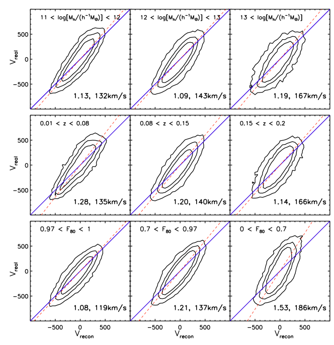
Figure 1.— Validations with mocks: true group velocities, $v_{\rm real}$, obtained directly from the mock vs. the corresponding reconstructed velocity, $v_{\rm recon}$, obtained by applying our reconstruction method to the mock data in redshift space. Note that all of these velocities are along the line of sight. The top and middle rows show results for galaxies in different halo mass and redshift bins, respectively, while the panels in the bottom row show results for different bins in the filling factor, $F_{80}$. The contours in each panel encompass $50\%$, $70\%$, and $85\%$ per cent of the groups in each subsample. The slope of the best-fitting relation and the scatter, in terms of the rms in $v_{\rm real}-v_{\rm recon}$, are also indicated in each panel.

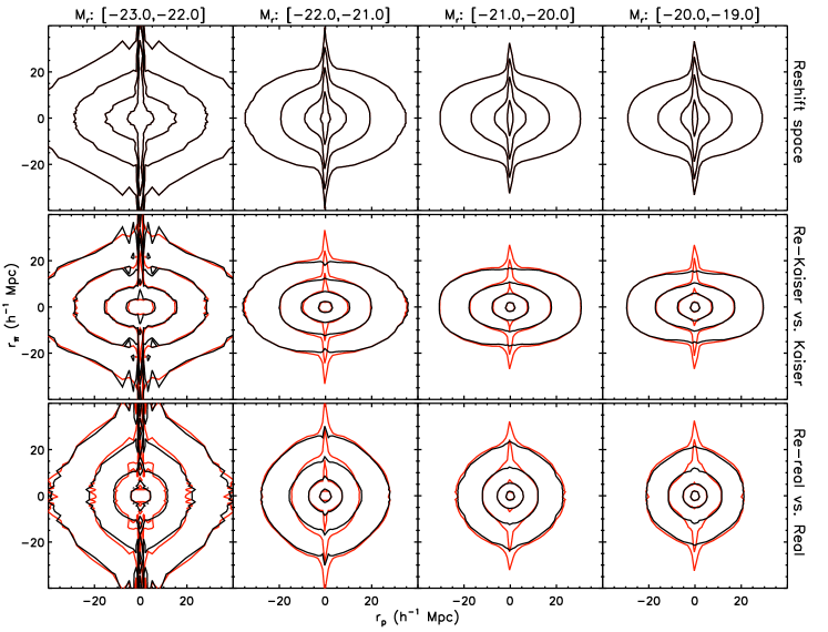
Figure 2.— Validations with mocks: comparison of two-dimensional 2PCFs of mock galaxies. Different columns correspond to mock galaxies in different absolute $r$-band magnitude bins, as indicated at the top of each column. Different rows correspond to different spaces, as indicated at the right of each row. Black and red contours correspond to the results in the true and reconstructed spaces, respectively, with contour levels corresponding to $\xi=5,~{}1,~{}0.3,~{}0.1$.

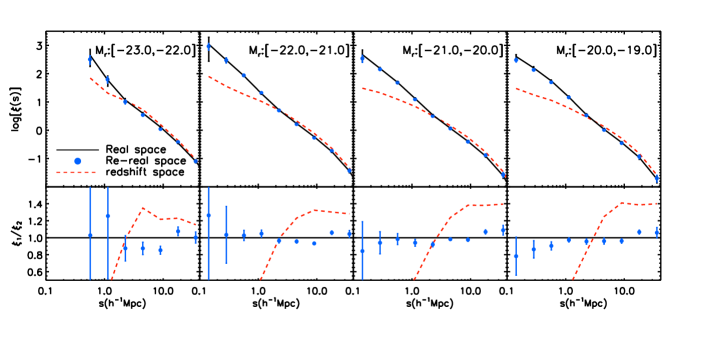
Figure 3.— Validations with mocks: 2PCFs (upper panels) and 2PCF ratios (lower panels) for mock galaxies in real vs. re-real space. The solid line in the upper panels indicates the 2PCF in the real space, averaged over 10 mock samples, while the blue filled circles indicate the corresponding average 2PCF in the re-real space, with the error bars indicating the $\pm 1\sigma$ variance among the 10 mock samples. The red dashed lines indicate the corresponding 2PCFs in redshift space and are shown for comparison. The lower panels plot the average and $\pm 1\sigma$ variance of the ratio of the 2PCFs in the re-real space over that in the real space (blue filled circles with error bars). The red dashed lines indicate the ratio of the redshift-space 2PCF to the real-space one. Different columns correspond to different $r$-band magnitude bins, as indicated.

3. Validation with Mock Data

In order to test and validate the method described above, we first apply it to a mock SDSS DR7 galaxy catalog. Although W12 and S16 already presented several tests regarding the reconstruction of the velocity field and the real-space correlation function, here we focus specifically on testing the application of our reconstruction method to a flux-limited sample.

3.1. Mock Catalogs

The mocks that we use here are exactly the same as those used in S16. For completeness, though, we briefly describe the main ingredients in what follows. The mocks are constructed from a high-resolution N-body simulation that evolves the distribution of $3072^{3}$ dark matter particles in a periodic box of $500\>h^{-1}{\rm{Mpc}}$ on a side (Li et al., 2016). This simulation was carried out at the Center for High Performance Computing at Shanghai Jiao Tong University and was run with L-GADGET, a memory-optimized version of GADGET2 (Springel, 2005). The cosmological parameters adopted by this simulation are consistent with the WMAP9 results (Hinshaw et al., 2013). Dark matter halos are identified using the standard friends-of-friends (FoF) algorithm (e.g. Davis et al., 1985) with a linking length that is 0.2 times the mean interparticle separation. Mock galaxies are assigned to dark matter halos using the conditional luminosity function (hereafter CLF, see Yang et al., 2003) as constrained by Cacciato et al. (2013). The algorithm used to assign luminosities and phase-space coordinates to the mock galaxies is similar to that used in Yang et al. (2004), and is described in detail in S16 (see also Lu et al., 2015).

Next, we proceed to construct mock galaxy samples that have the same survey selection effects as the SDSS DR7 (introduced in Section 2). We stack the populated simulation boxes in order to cover the volume of SDSS DR7. We then place a virtual observer at the center of the stack of boxes and remove all mock galaxies that are located outside of the SDSS DR7 survey region under a $(\alpha,\delta)$-coordinate system. Each galaxy is assigned the redshift and $r$-band apparent magnitude according to its distance, line-of-sight velocity, and luminosity and selected according to the position-dependent magnitude limit. To mimic the position-dependent completeness, we randomly sample each galaxy using the completeness masks provided by the SDSS DR7. We restrict the sample to galaxies within the redshift range $0.01\leq z\leq 0.2$ and with completeness $\geq 0.7$. Finally, in order to have a rough estimate of the cosmic variance, we construct a total of 10 such mock samples by randomly rotating and shifting the boxes in the stack. From each mock sample, four flux-limited subsamples are constructed using the redshift and absolute magnitude ranges listed in Table 1.

3.2. Testing the Reconstruction of the Velocity Field

We start by testing the velocity field reconstructed in the flux-limited sample. As mentioned in §2.2, since the groups are distributed in redshift space, the reconstruction needs to be iterated. As in W12, in order to facilitate a comparison with the real-space velocity field (in the mock data cube), we first use two iterations with our fiducial smoothing scale of ${\rm log}(M_{\rm s}/\>h^{-1}\rm M_{\odot})=14.75$. Next, we apply a third iteration, this time adopting a somewhat smaller smoothing scale of ${\rm log}(M_{\rm s}/\>h^{-1}\rm M_{\odot})=14.0$. This third iteration results in a weaker suppression of the (non)linear velocities, thereby giving a larger dynamic range over which the reconstruction of the velocity field can be tested.

Fig. 1 shows the comparison between the true group velocities, $v_{\rm real}$, in the simulation used to construct the mock and the velocities $v_{\rm recon}$, obtained from the reconstruction (using the three iterations described above). The slope of the best-fitting relation and the rms error between $v_{\rm real}$ and $v_{\rm recon}$ are indicated in each panel. Perfect reconstruction would correspond to unity slope and zero rms. Panels in the top and middle rows show results for groups in different halo mass bins and at different redshifts, respectively. Reconstructed velocities are linearly correlated with the true velocities, indicating overall success for the reconstruction method. However, there is appreciable scatter, which increases (weakly) with group mass and redshift. This is mainly due to the flux-limited nature of the sample used, which ensures that more massive halos are located at higher redshift, where the sampling of the density field is less accurate (mainly because $M_{\rm th}$ is larger). In addition to the scatter, there is a systematic bias, in that the slope of the $v_{\rm real}-v_{\rm recon}$ relation deviates from unity. In particular, for high values of $|v_{\rm real}|$, the corresponding $|v_{\rm recon}|$ is typically too small. This is mainly an effect of the limited volume that is used to probe the density field; recall that the velocity field is particularly sensitive to the large-scale modes. In order to quantify this effect, we follow W12 and compute for each group the ‘filling factor’ $F_{80}$, which is defined as the fraction of grid cell centers in a spherical volume of radius $80\>h^{-1}{\rm{Mpc}}$ centered on the group. Hence, $F_{80}\ll 1$ for a group that is close to the edge of the survey, while groups that are located more than $80\>h^{-1}{\rm{Mpc}}$ away from any survey boundary will have $F_{80}\sim 1$. The three panels in the bottom row of Fig. 1, show the results for groups split by $F_{80}$, as indicated. Note that we have arranged the split so that each of the three subsamples contains roughly an equal number of groups. For groups with $F_{80}\geq 0.97$, the reconstructed velocity is very accurate; the slope is close to unity, and the scatter is relatively small. As $F_{80}$ decreases, the slope of the correlation deviates more strongly from unity, while the scatter increases. Hence, the main limiting factor for the velocity reconstruction is the limiting volume probed by the SDSS data.

3.3. Testing the Clustering of Galaxies in Reconstructed Spaces

In order to gauge the accuracy of the correction method using the flux-limited sample, we now compare the clustering of galaxies in the reconstructed spaces with that in the corresponding true spaces. The method that we use to compute the 2PCFs is described in the Appendix.

We first start with a qualitative, visual comparison based on the 2D 2PCF ${\xi(r_{\rm p},r_{\pi})}$, shown in Fig. 2. Each column corresponds to a specific magnitude bin, as indicated at the top of each column. From top to bottom, the different rows show the results in different spaces, as indicated to the right of each row. In each case, black and red contours correspond to the true and reconstructed space, respectively. The ${\xi(r_{\rm p},r_{\pi})}$ in redshift space is clearly anisotropic, revealing the FOG effect on small scales and the impact of the Kaiser effect on large scales. The panels in the middle row demonstrate that the correction for the FOG compression (giving rise to re-Kaiser space) is fairly successful, except for some residual FOG effects at small projected separations. As discussed in S16, these shortcomings of the FOG compression arise from imperfections in the group finder and are virtually impossible to avoid with any group finder (see Campbell et al., 2015, for details). In fact, for FOG compression, there is no distinction as to whether the flux- or volume-limited sample is used. After correcting for both RSDs, the ${\xi(r_{\rm p},r_{\pi})}$ in re-real space (bottom row) is clearly more isotropic, showing that the correction for the Kaiser effect is fairly accurate, even for a flux-limited sample. Once again, the residual FOG effects are evident, but overall, the method appears to correct for most of the RSD.

A more quantitative estimate can be obtained using the one-dimensional 2PCF ${\xi(s)}$. Fig. 3 compares ${\xi(s)}$ in re-real space (blue filled circles) to that in real space (solid lines). Different columns correspond to different magnitude bins, as indicated. The upper panels show the actual 2PCFs obtained by averaging results from all 10 mocks, while the lower panels plot $\xi_{\rm re-real}/\xi_{\rm real}$. Error bars indicate the variance among the 10 mock samples and reflect the measurement error due to cosmic variance in an SDSS-like survey. The red dashed lines show the results in redshift space and are shown to emphasize the magnitude of the RSDs, as well as the success of our reconstruction method. Clearly, the correlation functions in re-real space are in excellent agreement with those in real space, with the vast majority of data points being consistent with $\xi_{\rm recon}/\xi_{\rm true}=1$ within $1\sigma$. For faint galaxies, the reconstructed 2PCF is systematically underpredicted on small scales, albeit at a barely significant level. This is a manifestation of the residual FOG effects arising from inaccuracies in the group finder. Overall, it is clear that the majority of RSDs have been successfully corrected. In particular, a comparison with Fig. 5 in S16 shows that the reconstruction presented here based on flux-limited samples is at least as accurate as that based on volume-limited samples.

4. Estimation of the structure Growth Rate

We now turn to our basic goal: measuring the structure growth rate $f\sigma_{8}$ using intermediate-scale clustering measurements. It is well known that modeling RSDs can be used to estimate the value of $\beta\equiv f/b$ (e.g. Peacock et al., 2001; Hawkins et al., 2003; Percival et al., 2004). Here we present a new method that can provide simultaneous measurements of $\xi(s)$, $f\sigma_{8}$ (the parameter of interest), and $b\sigma_{8}$ (the bias parameter). The idea is as follows. Our reconstruction depends (strongly) on cosmology and especially on the value taken by $f\sigma_{8}$. The reconstruction gives us both the 2PCF ${\xi(s)}$ in re-real space and the two-dimensional ${\xi(r_{\rm p},r_{\pi})}$ in re-Kaiser space (i.e., ${\xi(r_{\rm p},r_{\pi})}$ with FOG compression). By comparing ${\xi(s)}$ to the (cosmology-dependent) matter-matter correlation function on large scales, we can infer $b\sigma_{8}$, and thus $\beta=f/b$. Using linear theory, we can then use ${\xi(s)}$ and this value for $\beta$ to predict the two-dimensional 2PCF ${\xi(r_{\rm p},r_{\pi})}$ in the absence of the FOG effect, which can be compared directly to ${\xi(r_{\rm p},r_{\pi})}$ in re-Kaiser space obtained from our reconstruction. Only if the correct cosmology is used will these two correlation functions agree, thereby giving us a handle to constrain cosmological parameters, i.e., the linear growth rate parameter $f\sigma_{8}$.

In this section, we first give a detailed description of the method, and then we test it against mock galaxy samples.

4.1. Methodology

One of the key ingredients in our method to constrain the linear growth rate $f\sigma_{8}$ is the relation between ${\xi(r_{\rm p},r_{\pi})}$ and ${\xi(s)}$ in the absence of nonlinear FOG effects. According to linear theory, developed by Kaiser (1987) and Hamilton (1992), we can define ${\xi_{\rm mod}(r_{\rm p},r_{\pi})}$ as

$${\xi_{\rm mod}(r_{\rm p},r_{\pi})}=\xi_{0}(s){\cal P}_{0}(\mu)+\xi_{2}(s){\cal P}_{2}(\mu)+\xi_{4}(s){\cal P}_{4}(\mu)$$ (6)

Here ${\cal P}_{l}(\mu)$ is the $l^{\rm th}$ Legendre polynomial, $\mu$ is the cosine of the angle between the line of sight and the redshift-space separation $\bm{s}$, and the angular moments can be written as

$$\xi_{0}(s) = \left(1+\frac{2\beta}{3}+\frac{\beta^{2}}{5}\right){\xi(s)}$$ (7)

$$\xi_{2}(s) = \left(\frac{4\beta}{3}+\frac{4\beta^{2}}{7}\right)\left[{\xi(s)}-\bar{\xi}(s)\right]$$

$$\xi_{4}(s) = \frac{8\beta^{2}}{35}\left[{\xi(s)}+\frac{5}{2}\bar{\xi}(s)-\frac{7}{2}\hat{\xi}(s)\right]$$

with

$$\bar{\xi}(s) = \frac{3}{r^{3}}\int_{0}^{r}{\xi_{(}s^{\prime})s^{\prime 2}ds^{\prime}}$$ (8)

$$\hat{\xi}(s) = \frac{5}{r^{5}}\int_{0}^{r}{\xi_{(}s^{\prime})s^{\prime 4}ds^{\prime}}.$$

Note that $\beta\equiv f/b\equiv f\sigma_{8}/b\sigma_{8}$, where $f\sigma_{8}$ is the same growth rate parameter as used in the reconstruction and $b\sigma_{8}$ is the linear bias of the galaxies, which is defined by

$$\xi_{\rm gg}(s)=b^{2}\,\xi_{\rm mm}(s)=(b\sigma_{8})^{2}\,\xi_{\rm mm,\sigma_{8}=1.0}(s)\,,$$ (9)

where $\xi_{\rm gg}$ and $\xi_{\rm mm}$ are the correlation functions of galaxies and mass on large scales, respectively.

Figure 4.— Bias factor (top panels) and bias ratios (bottom panels) as a function of the absolute magnitude for mock galaxies (left panels) and SDSS galaxies (right panels). Here results are shown for a fixed $\sigma_{8}=0.817$. The bias factor is defined as the ratio of the measured re-real-space ${\xi(s)}$ to that of dark matter over the range $4\>h^{-1}{\rm{Mpc}}<s<20\>h^{-1}{\rm{Mpc}}$. Blue, black, and red solid lines correspond to cosmologies with $\Omega_{\rm m}=0.1,0.3,0.5$, respectively. The bias ratios are normalized to those for $\Omega_{\rm m}=0.1$. The error bars correspond to the $1\sigma$ variance among 10 mocks. For clarity, the error bars are only plotted for the biases of $\Omega_{\rm m}=0.3$. The dashed lines in the left panels correspond to the true bias, as measured in our mock real space, which has $\Omega_{\rm m}=0.282$.

Figure 5.— Validation with mocks, impact of cosmology: comparison of the modeled ${\xi_{\rm mod}(r_{\rm p},r_{\pi})}$ (red lines) and the measured ${\xi_{\rm mea}(r_{\rm p},r_{\pi})}$ in re-Kaiser space (black lines). Different rows correspond to the ${\xi_{\rm mod}(r_{\rm p},r_{\pi})}$ with different $\Omega_{\rm m}$, as indicated to the right of each row. Different columns correspond to different absolute magnitude bins, as indicated at the top of each column. Contour levels correspond to $\xi=0.3,~{}0.1,~{}0.05,~{}0.02$. Here again, results are shown for a fixed $\sigma_{8}=0.817$.

In summary, our method for simultaneously constraining the growth rate $f\sigma_{8}$ and the real-space 2PCF $\xi(s)$ (including bias parameter $b\sigma_{8}$) consists of the following steps.

1. Pick a set of cosmological parameters and compute the corresponding value for $f\sigma_{8}$. In practice, we use the fitting function of Lahav et al. (1991):

   $$f(z)\simeq\Omega_{\rm m}^{0.6}(z)+\frac{1}{70}\Omega_{\Lambda}(z)\left[1+\frac{\Omega_{\rm m}(z)}{2}\right].$$ (10)

2. Reconstruct the velocity field using the flux-limited group sample.

   1. Run the group finder over the data. Since this involves measuring distances and absolute magnitudes, this step is cosmology-dependent, as are all subsequent steps below.

   2. Assign halo masses to the groups using rank-order matching onto the characteristic group luminosity (see §2 for details).

   3. For each redshift range listed in Table 2, determine $M_{\rm th}$ and compute the corresponding $b_{\rm hm}$ using Eq. (4).

   4. Apply the reconstruction method, which consists of the following steps: (i) Fourier transform the density field $\delta(\bm{x})=\delta_{\rm h}(\bm{x})/b_{\rm hm}$, (ii) compute $\bm{v}(\bm{k})$ using Eq. (2), and (iii) Fourier transform $\bm{v}(\bm{k})$ to obtain the velocity field $\bm{v}_{\rm cen}(\bm{x})$. As discussed in §2.2, we iterate this process until convergence is achieved.

3. Measure the 2PCF in re-Kaiser space and re-real space.

   1. Apply the statistical FOG compression using the method described in §2.2, and compute the two-dimensional 2PCF in re-Kaiser space, which we denote by ${\xi_{\rm mea}(r_{\rm p},r_{\pi})}$.

   2. Correct for the Kaiser effect by reassigning galaxies their corrected redshifts, given by Eq. (5). Compute the corresponding comoving distances and use these to compute the 2PCF ${\xi(s)}$ in re-real space.

4. Estimate ${\xi_{\rm mod}(r_{\rm p},r_{\pi})}$

   1. Compute the galaxy bias parameter $b\sigma_{8}$, using Eq. (9) applied to the separation range $4\>h^{-1}{\rm{Mpc}}<s<20\>h^{-1}{\rm{Mpc}}$. Throughout, $\xi_{\rm mm}(s)$ is computed from the nonlinear matter power spectrum using the method of Smith et al. (2003) and adopting the transfer function of Eisenstein & Hu (1998).

   2. Compute $\beta=f/b$, and use this together with ${\xi(s)}$ to compute ${\xi_{\rm mod}(r_{\rm p},r_{\pi})}$ using Eq. (6).

5. In order to quantify the level of agreement between ${\xi_{\rm mod}(r_{\rm p},r_{\pi})}$ and ${\xi_{\rm mea}(r_{\rm p},r_{\pi})}$ we compute

   $$\chi^{2}=\sum{\left[\frac{{\xi_{\rm mod}(r_{\rm p},r_{\pi})}-{\xi_{\rm mea}(r_{\rm p},r_{\pi})}}{\sigma}\right]^{2}}.$$ (11)

   Here $\sigma$ is the rms of ${\xi_{\rm mea}(r_{\rm p},r_{\pi})}$ determined from each of our 10 mock samples, and the summation is over a total of $4\times 31$ logarithmic bins in $r_{\rm p}$ (spanning the range $10\>h^{-1}{\rm{Mpc}}<r_{\rm p}<60\>h^{-1}{\rm{Mpc}}$) and $r_{\pi}$ (spanning the range $0.06\>h^{-1}{\rm{Mpc}}<r_{\pi}<80\>h^{-1}{\rm{Mpc}}$). In order to allow for a fair comparison among the different sets of realizations, we always use the same $\sigma$, which has been obtained for the WMAP9 cosmology.

6. We repeat steps 1-5 to search for the set of cosmological parameters that yields the minimum $\chi^{2}$ value.

Note that in computing $\chi^{2}$, we exclude all data with $r_{\rm p}<10\>h^{-1}{\rm{Mpc}}$. The reason is twofold. First of all, there are still residual FOG effects in re-Kaiser space that show up on small scales (cf. Fig. 2). Second, the linear theory prediction of Eq. (6) becomes inaccurate on small, quasi-linear scales ($\lower 3.01385pt\hbox{$\;\buildrel<\over{\sim}\;$}8\>h^{-1}{\rm{Mpc}}$; Reid et al., 2014). We find that including data on smaller scales by reducing the lower limit of $r_{\rm p}$, increases the $\chi^{2}$. Focusing on larger scales by increasing the lower limit of $r_{\rm p}$ results in noisier, less accurate constraints. Following multiple tests, we found the choice of $r_{\rm p}<10\>h^{-1}{\rm{Mpc}}$ to be a good compromise between these two effects.

Note that cutting results below $r_{\rm p}=10\>h^{-1}{\rm{Mpc}}$ does not mean that one can ignore the FOG compression when computing ${\xi_{\rm mea}(r_{\rm p},r_{\pi})}$. The FOG effect caused by the nonlinear velocities on small scales has significant impact on the large-scale clustering of galaxies. This is evident from Fig. 2, which reveals clear differences between ${\xi(r_{\rm p},r_{\pi})}$ in redshift space and in Kaiser space out to large $r_{\rm p}$. Hence, it is necessary to compress the FOG effects, even when only modeling the linear ${\xi(r_{\rm p},r_{\pi})}$ on large scales ($r_{\rm p}>10\>h^{-1}{\rm{Mpc}}$). We will explicitly demonstrate this in the next section.

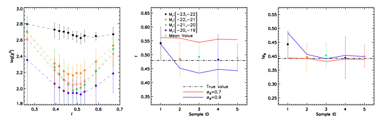
Figure 6.— Validations with mocks: left panel shows $\log(\chi^{2})$ as a function of ${f(\Omega_{\rm m})}$. This $\chi^{2}$ is computed using Eq. (11) using the ${\xi_{\rm mea}(r_{\rm p},r_{\pi})}$ measured in re-Kaiser space and assuming the same value for $\sigma_{8}$ ($0.817$) as in the simulation used to construct the mocks. Filled circles show results for galaxies in four different magnitude bins as indicated with different colors, while error bars indicate the $\pm 1\sigma$ variance among our 10 mocks. Diamonds show the corresponding results averaged over the three faintest samples. Dashed lines are simple polynomials fit to these $\chi^{2}(f)$ results. The middle panel shows the best-fitting $f$ in different magnitude samples (circles) and the corresponding averaged results (diamond). The sample IDs ($x$-axis, from 1 to 4) used in the middle and right panels correspond to the ones listed in Tabel 1, while sample 5 is for the average results based on the mean value of $\chi^{2}$ for the samples 2-4. The dot-dashed line indicates the true value of $f$ in the simulation. The red and blue solid curves show the best-fitting $f$ obtained assuming $\sigma_{8}=0.7$ and 0.9, respectively. The right panel is similar to the middle panel but for $f\sigma_{8}$ values.

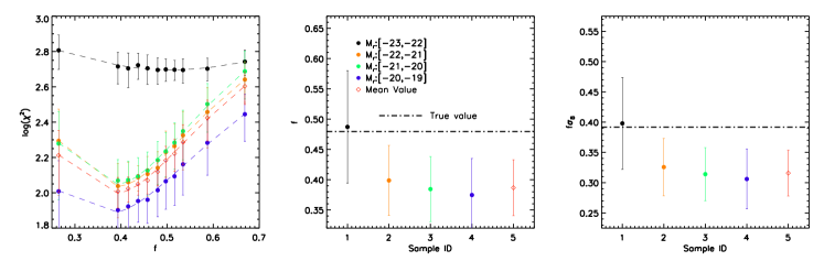
Figure 7.— Validations with mocks: same as Fig. 6 but here $\chi^{2}$ is computed using ${\xi_{\rm mea}(r_{\rm p},r_{\pi})}$ measured in redshift space, rather than in re-Kaiser space. Note that not including FOG compression results in significantly biased inferences, even when excluding data with $r_{\rm p}<10\>h^{-1}{\rm{Mpc}}$

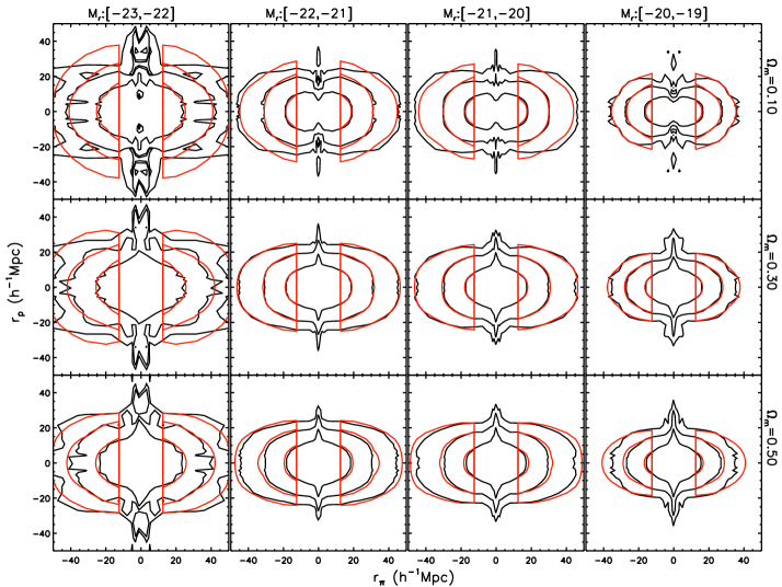
Figure 8.— Application to SDSS: comparison of the modeled ${\xi_{\rm mod}(r_{\rm p},r_{\pi})}$ (red lines) and the measured ${\xi_{\rm mea}(r_{\rm p},r_{\pi})}$ in re-Kaiser space (black lines) for SDSS DR7 data. Different rows correspond to the ${\xi_{\rm mod}(r_{\rm p},r_{\pi})}$ with different $\Omega_{\rm m}$, as indicated to the right of each row. Different columns correspond to different absolute magnitude bins, as indicated at the top of each column. Contour levels correspond to $\xi=0.3,~{}0.1,~{}0.05$.

4.2. Tests Based on Mock Data

In order to test the method outlined above, we use the mock data described in §3.1, which is based on a cosmological $N$-body simulation that adopts the WMAP9 cosmology with $\Omega_{\rm m}=0.282$ and $\sigma_{8}=0.817$. The corresponding value for $f$ is $0.48$, which we refer to as the ‘true’ value. Since the velocity field depends on a combination of $f$ and $\sigma_{8}$, in our investigation, we will use a fixed $\sigma_{8}=0.817$ at first and change to other $\sigma_{8}$ values at the second stage. We analyze the mock data assuming 11 different values of $\Omega_{\rm m}$: $0.10$, $0.20$, $0.22$, $0.24$, $0.26$, $0.28$, $0.30$, $0.32$, $0.34$, $0.40$, and $0.50$. The corresponding values for $f$ range from $0.265$ to $0.669$. In each case, we adjust $\Omega_{\Lambda}$ accordingly so as to assure a flat cosmology ($\Omega_{\rm m}+\Omega_{\Lambda}=1$), while all other cosmological parameters are held fixed to the WMAP9 cosmology used for the simulation.

First, we test how well the method can recover the galaxy bias parameter $b$, and how the inferred value depends on the assumed value of $\Omega_{\rm m}$. The top left panel of Fig. 4 shows the bias factor $b$ as a function of galaxy luminosity. Solid lines indicate the results inferred from Eq. (9), where ${\xi(s)}$ is the correlation function of mock galaxies in the reconstructed re-real space, and $\xi_{\rm mm}(r)$ is the nonlinear matter 2PCF for the assumed cosmology (i.e., the assumed value of $\Omega_{\rm m}$, as indicated). For comparison, the dashed line indicates the bias factor $b$ inferred from Eq. (9) using the ‘true’ real-space 2PCF of mock galaxies and the 2PCF of the dark matter for the actual cosmology of the simulation. Hence, this bias factor basically represents the true bias of the mock galaxies. The error bars reflect the $1\sigma$ variance among the 10 mocks and are only plotted for the results for $\Omega_{\rm m}=0.3$ for clarity. The bottom left panel shows the ratios of the bias with respect to that for $\Omega_{\rm m}=0.1$. Note that all of these results correspond to $z=0.0$, which is the redshift of the simulation output that we used to construct the mock data.

It is reassuring that the reconstructed real-space bias $b$ best matches the ‘true’ bias for $\Omega_{\rm m}=0.3$, which is the value that is closest to the actual value used in the simulation ($0.282$). Adopting $\Omega_{\rm m}=0.1$ ($0.5$) results in an inferred bias that is systematically too low (high). We thus conclude that our method can adequately recover the bias parameter as long as the assumed cosmology is correct, while an incorrect cosmology results in a systematic error in the inferred bias (see also S16 for additional tests).

Next, we compare ${\xi_{\rm mea}(r_{\rm p},r_{\pi})}$ with the corresponding model prediction, ${\xi_{\rm mod}(r_{\rm p},r_{\pi})}$. As discussed above, an incorrect cosmology results in a value for $f$ ($f\sigma_{8}$) that deviates from the true value, which in turn will introduce systematic errors in ${\xi_{\rm mod}}$. Fig. 5 shows the comparison between ${\xi_{\rm mod}}$ (red lines) and ${\xi_{\rm mea}}$ (black lines). Different rows show the ${\xi_{\rm mod}}$ inferred for three different cosmologies, $\Omega_{\rm m}=0.1,~{}0.3,~{}0.5$, from top to bottom. Different columns correspond to different magnitude bins, as indicated at the top of each column. As for the bias parameter $b$, the results for $\Omega_{\rm m}=0.3$, which is closest to the real value, are in better agreement with ${\xi_{\rm mea}}$, at least for the three fainter magnitude bins. For the brightest magnitude bin, the results for $\Omega_{\rm m}=0.5$ actually appear to give a better match on large scales, but the results for this magnitude bin are quite noisy due to the low number density of brighter galaxies.

In order to make this more quantitative, we now focus on the $\chi^{2}$ values defined by Eq. (11). The left panel of Fig. 6 plots the logarithm of $\chi^{2}$ as a function of $f$. Filled, colored circles correspond to different absolute magnitude bins, as indicated, while error bars reflect the $\pm 1\sigma$ variance among the 10 mock samples. Clearly, in the three faint bins, there is a significant, consistent minimum value for $\chi^{2}$, indicating a best-fitting $f$. For the brightest magnitude bin, though, the minimum is less pronounced and shifts to higher values of $f$. The open diamonds show the mean value averaged over the three faintest bins. The middle panel of Fig. 6 shows the best-fitting $f$ for each of our four magnitude bins (filled circles), obtained by fitting a polynomial to the $\chi^{2}(f)$ relation (shown as dashed lines in the left panel). The open diamond shows the best fit based on the mean value of $\chi^{2}$ for the three faintest bins. Error bars reflect the $1\sigma$ variance determined from each of our 10 mocks. For comparison, the dot-dashed line indicates the true value of $f$. Clearly, our best-fit values for $f$ are in excellent agreement with this true value, except for the brightest magnitude bin, which is biased toward a higher value. The mean inferred $f$ from the three faint bins is $0.488\pm 0.046$. Given that the true value of $f$ is $0.48$, we thus conclude that our method, when applied to an SDSS-like survey, is able to infer an unbiased estimate of the growth rate parameter $f$ to an accuracy of $\sim 10\%$.

Having tested the performance of our constraints on $f$ using the true $\sigma_{8}$ value ($\sigma_{8}=0.817$), we proceed to probe the impact of using different $\sigma_{8}$ values. Assuming $\sigma_{8}=0.7$ and $0.9$, we perform the same procedures that we applied for our fiducial $\sigma_{8}=0.817$ case to constrain the related $f$ values. The results are indicated by the red and blue lines in the middle panel of Fig. 6, which show that lowering $\sigma_{8}$ systematically increases the model prediction for $f$, and vice versa. This behavior is expected from the fact that the velocity field is governed by $f\sigma_{8}$ (see Eq. 3). This is confirmed by the right panel of Fig. 6, which shows that our method yields predictions for the product $f\sigma_{8}$ that are, to good approximation, independent of $\sigma_{8}$. Note that since we have used three different values of $\sigma_{8}$, each with 10 mocks, the error bars shown here are estimated to reflect the $1\sigma$ uncertainty of $f\sigma_{8}$ among all the 30 data values.

Finally, as already alluded to in the previous subsection, it is important to include FOG compression, even when excluding data with $r_{\rm p}<10\>h^{-1}{\rm{Mpc}}$. To make this evident, Fig. 7 shows the equivalent of Fig. 6, but this time the $\chi^{2}$ is computed using ${\xi_{\rm mea}(r_{\rm p},r_{\pi})}$ measured in redshift space, rather than re-Kaiser space. Although the brightest magnitude bin now yields inferred $f$ and $f\sigma_{8}$ that are consistent with the true values, albeit with large error bars, the best-fit values of $f$ and $f\sigma_{8}$ inferred from the three fainter magnitude bins are systematically and significantly biased toward lower value. Note that our sampling of $f$ is actually inadequate (it is unclear whether we have sampled the true minimum of $\chi^{2}(f)$). Consequently, if anything, we are likely to have overestimated the best-fit values for $f$ and $f\sigma_{8}$.

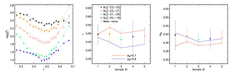
Figure 9.— Measurement of $f$ based on SDSS DR7 data. This figure is the same as Fig. 6, but here we have applied our method to the sample of $584,473$ SDSS DR7 galaxies in the NGC (see Section 2).

5. Application to the SDSS

Having demonstrated that our reconstruction method is also applicable to flux-limited samples and that we can accurately constrain the growth rate parameter $f\sigma_{8}$, we now apply our method to all galaxies in the NGC region of the SDSS DR7. As described in Section 2, this sample contains 584,473 galaxies with $z_{\rm med}=0.1$.

5.1. Measurement of $f\sigma_{8}$

We now apply our six-step iterative method, outlined in Section 4.1, to the SDSS data, using a set of cosmologies (i.e., different $\Omega_{\rm m}$ values). We start by keeping the value for $\sigma_{8}$ fixed to $0.817$. The right panels of Fig. 4 show the bias factor and bias ratios as a function of the absolute magnitude for SDSS galaxies. In agreement with the mock results, larger values for $\Omega_{\rm m}$ result in larger inferred values for the bias parameter $b$.

Fig. 8 shows the comparison between ${\xi_{\rm mea}}$ and ${\xi_{\rm mod}}$ for three cosmologies with $\Omega_{\rm m}=0.1$, $0.3$, and $0.5$, in different rows. Different columns correspond to the four absolute magnitude bins, $\bm{[}-23.0,-22.0\bm{]}$, $\bm{[}-22.0,-21.0\bm{]}$, $\bm{[}-21.0,-20.0\bm{]}$, and $\bm{[}-20.0,-19.0\bm{]}$, as indicated at the top of each column. Black and red lines correspond to ${\xi_{\rm mea}}$ and ${\xi_{\rm mod}}$, respectively. Clearly, the ${\xi_{\rm mod}}$ based on $\Omega_{\rm m}=0.3$ is in good agreement with the corresponding ${\xi_{\rm mea}}$, while for $\Omega_{\rm m}=0.1$ and $0.5$, there are clear systematic discrepancies.

The left panel of Fig. 9 shows $\chi^{2}$ as a function of the value of $f$ for the assumed cosmology. Filled, colored circles correspond to different absolute magnitude bins, while the open diamonds show the mean values obtained by combining the three faintest bins. As for the mock data, $\chi^{2}(f)$ reveals clear minima from which we can infer constraints on $f$. The middle panel of Fig. 9 shows the best-fitting $f$ for the different magnitude bins. Error bars indicate the $\pm 1\sigma$ variance among the 10 mock samples described in Section 4.2. As one can see, the values of the best-fitting $f$ in all four magnitude bins are consistent with each other to better than $1\sigma$. Based on our mock results, though, we exclude the brightest magnitude bin from our final constraint on $f$, which we base on the mean $\chi^{2}$ for the three faintest bins (indicated by the open diamond). This yields a best-fit value for the growth rate parameter of $f(z_{\rm med}=0.1)=0.484\pm 0.049$. As always, the error bar indicates the $1\sigma$ variance among the 10 mock samples.

As for the mocks, we now test the impact of $\sigma_{8}$ on our constraints for $f$ and $f\sigma_{8}$ by fixing $\sigma_{8}=0.7$ and 0.9, respectively. For each $\sigma_{8}$, we repeat the measurement of $f$ using the method described in Section 4.1. The best-fitting $f$ values are shown in the middle panel of Fig. 9. Red and blue solid curves correspond to $\sigma_{8}=0.7$ and $0.9$, respectively. As for the mocks, the values for $f$ systematically and significantly increase (decrease) with increasing (decreasing) $\sigma_{8}$. However, as shown in Eq. (3) and tested with mock samples, $f\sigma_{8}$ should be related to the unique velocity field in our universe and thus be independent of the value of $\sigma_{8}$ used in our analysis. The right panel of Fig. 9 shows that there is indeed good agreement between the $f\sigma_{8}$ values inferred assuming $\sigma_{8}=0.817$ (colored symbols) or $0.9$ (blue curve). Assuming $\sigma_{8}=0.7$ (red curve) yields values for $f\sigma_{8}$ that are somewhat lower, although the offset is small compared to the measurement errors (error bars, reflecting the $\pm 1\sigma$ variance among our 30 mock samples). Note that since the SDSS data correspond to a median redshift $z_{\rm med}=0.1$, here we have extrapolated $\sigma_{8}$ to its expected value at $z=0.1$ using $\sigma_{8}(z)=D(z)\sigma_{8}(z=0)$, with $D(z)$ the linear growth factor normalized to unity at $z=0$.

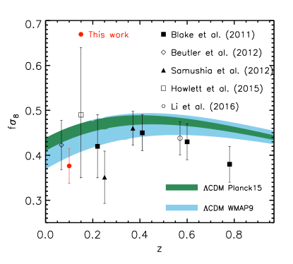
Figure 10.— Comparison of the growth of structure measured at different redshifts. Our result is shown as the red filled circle. Black symbols show results from various works, including those for 6dFGS (Beutler et al., 2012), the WiggleZ survey (Blake et al., 2011), and the SDSS (Samushia et al., 2012; Howlett et al., 2015; Li et al., 2016). The blue band shows the $1\sigma$ confidence level allowed by the WMAP9 parameters assuming a flat $\Lambda$CDM cosmology with GR. The green band shows the $1\sigma$ confidence level allowed by the Planck parameters (Planck Collaboration et al., 2015), also assuming a flat $\Lambda$CDM + GR cosmology.

Having demonstrated that our inferred value for $f\sigma_{8}$ is indeed independent of the assumed value for $\sigma_{8}$ (at the $1\sigma$ level), we now compare our constraints on $f\sigma_{8}$, as inferred under the assumption that $\sigma_{8}=0.817$, to constraints from previous studies. Our results imply that $f\sigma_{8}=0.376\pm 0.038$ at $z=0.1$ (open diamond in the right panel of Fig. 9). Fig. 10 compares this constraint on $f\sigma_{8}$ (red circle) with previous measurements spanning a range of redshifts. These include the results from the 6dFGS (Beutler et al., 2012), the WiggleZ survey (Blake et al., 2011), and various constraints from the SDSS (Samushia et al., 2012; Howlett et al., 2015; Li et al., 2016). The blue band shows the $1\sigma$ confidence level allowed by the WMAP9 parameters assuming a flat $\Lambda$CDM universe plus GR. The green band is the same but using the Planck parameters (Planck Collaboration et al., 2015). Our measurement is consistent with the WMAP9 prediction at the $1\sigma$ level and somewhat lower than the Planck $\Lambda$CDM$+$GR expectations.

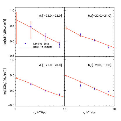
Figure 11.— The ESDs around lens galaxies in different absolute magnitude bins. The circles with error bars are the results obtained by Luo et al. (2017) from the galaxy-galaxy lensing shear measurements. The red lines are the model predictions for our best-fit $\Omega_{\rm m}/b$.

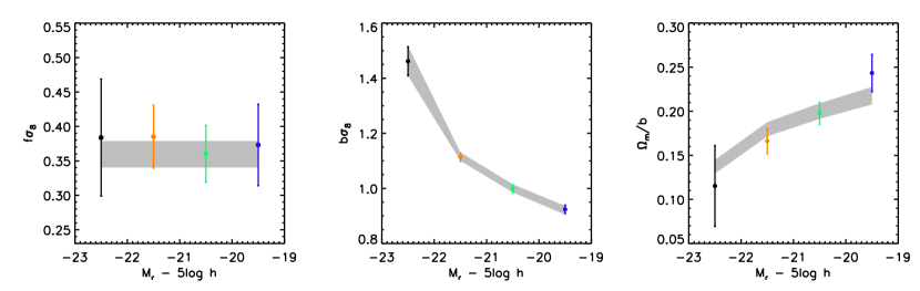
Figure 12.— The $f\sigma_{8}$ (left panel), $b\sigma_{8}$ (middle panel), and $\Omega_{m}/b$ (right panel) as a function of luminosity for SDSS DR7 data. The gray band reflects the $68\%$ confidence region predicted by the MCMC.

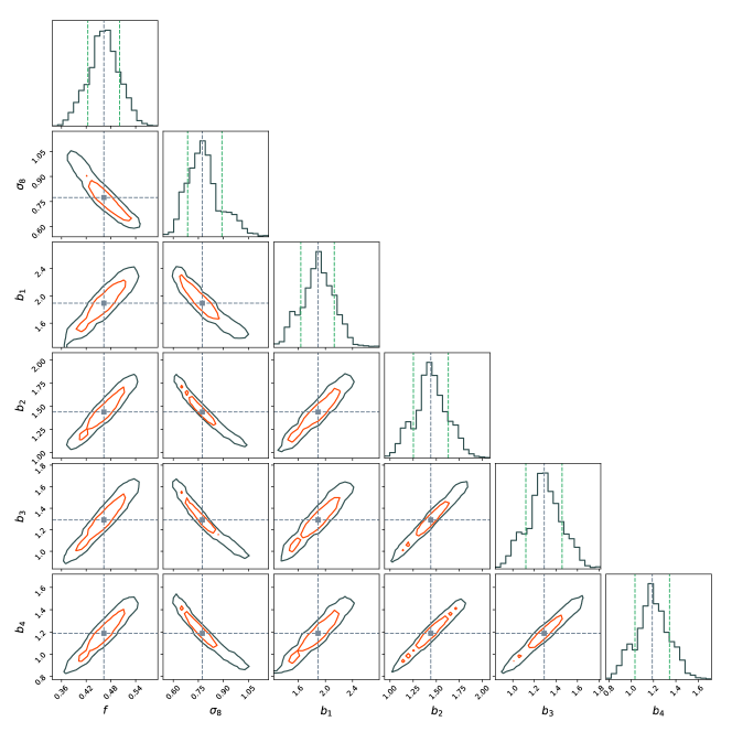
Figure 13.— Best fit (cross of dashed lines) and the projected distribution of the parameters in two-dimensional (2D) or one-dimensional (1D) space. The red and black contours in the 2D plane correspond to the boundaries of $68\%$ and $95\%$ confidence levels, respectively. The 1D distributions are the marginalized distributions of individual parameters. The vertical black and green dashed lines indicate the best-fitting values and the $68\%$ confidence region, respectively.

5.2. Constraints on $f$, $\sigma_{8}$, and $b$

In the previous subsection, we used real-space clustering data and RSDs to constrain $b\sigma_{8}$ and $f\sigma_{8}$, which both depend on the value of $\sigma_{8}$. We now complement these data with additional measurements that allow us to break the degeneracy among the three parameters $f$, $\sigma_{8}$ and $b$. In particular, we make use of galaxy-galaxy lensing data, which measure the excess surface density (ESD) of galaxy lenses using shear measurements of background source galaxies. The ESD is defined as

$$\Delta\Sigma(r_{\rm p})=\Sigma(\leq r_{\rm p})-\Sigma(r_{\rm p})=\gamma_{\rm t}\Sigma_{\rm crit}(z_{\rm l},z_{\rm s})\,,$$ (12)

where $\Sigma_{\rm crit}(z_{\rm l},z_{\rm s})=\frac{c^{2}}{4\pi G}\frac{D_{\rm s}}{D_{\rm l}D_{\rm ls}}$ is a geometry factor of the source and lens system. Here $\Sigma(\leq r_{\rm p})$ and $\Sigma(r_{\rm p})$ are the mean surface mass density inside of and at radius $r_{\rm p}$, respectively. The mean ESD around a lens galaxy is related to the line-of-sight projection of the galaxy-matter cross-correlation function, $\xi_{\rm gm}(r)$, as

$$\Sigma(r_{\rm p})={2\Omega_{\rm m}\rho_{\rm c}}\int_{r_{p}}^{\infty}\xi_{\rm gm}(r)\frac{r\,{\rm d}r}{\sqrt{r^{2}-r_{p}^{2}}}$$ (13)

and

$$\Sigma(\leq r_{\rm p})=\frac{2}{r_{p}^{2}}\int_{0}^{r_{p}}\Sigma(y)~{}y\,{\rm d}y$$ (14)

where $\rho_{\rm c}$ is the critical density of the universe. Since we have obtained reliable measurements of $\xi_{\rm gg}(r)$ in real space, we can predict the corresponding ESDs by rewriting Eq. 13 as follows:

$$\Sigma(r_{\rm p})=\frac{\Omega_{\rm m}}{b}{2\rho_{\rm c}}\int_{r_{p}}^{\infty}\xi_{\rm gg}(r)\frac{r\,{\rm d}r}{\sqrt{r^{2}-{r_{p}}^{2}}}\,,$$ (15)

where we have made the assumption that the cross-correlation coefficient $r=\xi_{\rm gm}/\sqrt{\xi_{\rm gg}\xi_{\rm mm}}$ is equal to unity (on our scales of interest). With these relations, we can use the galaxy-galaxy lensing measurements together with the real-space 2PCF measurements to obtain an independent measure of $\Omega_{\rm m}/b$.

In a recent study, Luo et al. (2017) used the background galaxies in the SDSS DR7 to measure ESDs around lens galaxies that are separated into the same luminosity bins as adopted here. The circles with error bars shown in Fig. 11 are their ESD measurements on relatively large scales in different absolute magnitude bins. The error bars shown on top of the circles are estimated using 2500 bootstrap resamplings of the lens galaxy samples, which are quite small and in general reflect the Poisson sampling errors.

Combing these ESD measurements, $\Delta\Sigma(r_{\rm p})$, with our measurements of the real-space 2PCF, $\xi_{\rm gg}(r)$, we now use Eqs.(12) - (15) to constrain the ratio $\Omega_{\rm m}/b$. Since $b$ is a scale-independent linear bias factor, which is only accurate at sufficiently large scales, we only use the $\Delta\Sigma(r_{\rm p})$ data over the radial range $2\>h^{-1}{\rm{Mpc}}<r_{\rm p}<10\>h^{-1}{\rm{Mpc}}$. On these large scales, the cross-correlation coefficient is also close to unity (e.g., Cacciato et al., 2012). We apply this method separately to each of our four magnitude bins, the results of which are shown in the right panel of Fig. 12. Error bars indicate our estimated errors on $\Omega_{\rm m}/b$, which are computed by propagating the errors on both $\xi_{\rm gg}(r)$ and $\Delta\Sigma(r_{\rm p})$.

By combining all our constraints on $\Omega_{\rm m}/b$, and $f\sigma_{8}$, and $b\sigma_{8}$ (shown, for completeness, in the left and middle panels of Fig. 12), we now derive constraints on the related parameters, $f$ (or $\Omega_{m}$) and $\sigma_{8}$, as well as the bias parameters, $b_{i}$ for each separate luminosity bin, $i$. To do so, we write

$$f\sigma_{8}=c_{i,1}\pm\sigma_{i,1}$$ (16)

$$b_{i}\sigma_{8}=c_{i,2}\pm\sigma_{i,2}$$ (17)

$$\frac{\Omega_{m}}{b_{i}}=c_{i,3}\pm\sigma_{i,3}$$ (18)

where $i$ denotes the magnitude bin ($i=1,2,3,4$), and $c_{i,1}$, $c_{i,2}$ and $c_{i,3}$ indicate the data values shown in the left, middle, and right panels of Fig. 12, respectively, the corresponding errors of which are $\sigma_{i,1}$, $\sigma_{i,2}$ and $\sigma_{i,3}$. Using these 12 measurements $(c_{i,j},\sigma_{i,j})$, where $i=1,2,3,4$ and $j=1,2,3$, we constrain the six free parameters ($\sigma_{8}$, $f$ $b_{1}$, $b_{2}$, $b_{3}$ and $b_{4}$), using a Monte Carlo Markov chain (MCMC) method to explore the likelihood function in the multidimensional parameter space. The corresponding $\chi^{2}$ is defined as

$$\chi^{2}\!=\!\!\!\sum_{i=1}^{4}\!\left[\!\left(\!\frac{f\sigma_{8}\!\!-c_{i,1}}{\sigma_{i,1}}\!\right)^{2}\!\!\!+\!\left(\!\frac{b_{i}\sigma_{8}\!\!-c_{i,2}}{\sigma_{i,2}}\!\right)^{2}\!\!\!+\!\left(\!\frac{\Omega_{m}/b_{i}\!\!-c_{i,3}}{\sigma_{i,3}}\!\right)^{2}\!\right]\,\!\!\!.\!\!$$ (19)

We start the MCMC from an initial guess that is consistent with the WMAP9 cosmology and run the MCMC for 100,000 steps. At any point in the chain, we generate a new set of model parameters by drawing the shifts in the six free parameters from six independent Gaussian distributions. The Gaussian variances are tuned so that the average acceptance rate for the new trial model is about 0.25, and we remove the first 10,000 models in the chain to correct for the burn-in phase. In order to suppress the correlation between neighboring models in the chain, we thin the chain by a factor of 10. This results in a final chain of 9000 independent models that sample the posterior distribution. Fig. 13 shows the projected two-dimensional boundaries in the parameter space. The best-fit values are indicated by the cross of the dashed lines. The red and black contours indicate the $68\%$ and $95\%$ confidence levels, respectively. Not surprisingly, many parameter pairs are strongly correlated, in particular $f$ and $\sigma_{8}$, as well as $b_{i}$ and $\sigma_{8}$. Fig. 13 also shows the marginalized, one-dimensional distributions for each parameter, with vertical black and green dashed lines indicating the mean and the $68\%$ confidence regions.

As an illustration, the solid lines in Fig. 11 show the ESD model predictions for our best-fit $\Omega_{\rm m}/b$ value. The error bars shown on top of the solid line are obtained from the $\xi_{\rm gg}(r)$ of 30 mock data points and reflect the cosmic variance. The model predictions agree extremely well with the direct measurements. In addition, the gray bands in Fig. 12 show the 68% confidence intervals from the posterior predictions for $f\sigma_{8}$ (left panel), $b\sigma_{8}$ (middle panel), and $\Omega_{\rm m}/b$ (right panel). Overplotted in color are our observational constraints for each of the four magnitude bins. As is evident, the posterior predictions are in good agreement with these constraints, indicating that the constraints are mutually consistent with each other and with a $\Lambda$CDM + GR cosmology. Combining RSDs with weak lensing data, we have thus been able to put successful constraints on the logarithmic derivative of the linear growth rate, $f$, on the clustering amplitude of matter, $\sigma_{8}$, and on the galaxy bias factor, $b$, for galaxies in four luminosity bins at a median redshift $z_{\rm med}=0.1$. For reference, Table 4 lists the best-fit parameters together with their $68\%$ confidence levels.

[c] $f$ $\sigma_{8}$ $b_{1}$ $b_{2}$ $b_{3}$ $b_{4}$ $0.464^{+0.040}_{-0.040}$ $0.769^{+0.121}_{-0.089}~{}$ $1.910^{+0.234}_{-0.268}$ $1.449^{+0.194}_{-0.196}$ $1.301^{+0.170}_{-0.177}$ $1.196^{+0.159}_{-0.161}~{}$ Notes. All of the best-fit parameters listed in this table correspond to the values at redshift $z_{\rm med}=0.1$. Note that $\sigma_{8}$ can be extrapolated to the value at $z=0$ using $\sigma_{8}(0)=\sigma_{8}(z=0.1)/D(z=0.1)$, with $D(z)$ the linear growth factor normalized to unity at $z=0$. The linear bias parameters $b_{1}$, $b_{2}$, $b_{3}$ and $b_{4}$ correspond to galaxies in absolute magnitude bins $\>{}^{0.1}{\rm M}_{r}-5\log h=[-23,0,-22.0],[-22,0,-21.0],[-21.0,-20.0]$, and $[-20.0,-19.0]$, respectively.

Table 4The Best-fit Parameter

6. Summary

In S16, we presented a new, reliable method to correct the RSDs in galaxy redshift surveys and successfully applied it to the SDSS DR7 data to construct a real-space version of the main galaxy catalog. This allows for an accurate, ‘direct’ measurement of the real-space correlation function. In this paper, the second in a series, we use the reconstructed galaxy distribution to constrain $f$ and $\sigma_{8}$, as well as the linear galaxy bias parameter, $b$, in different luminosity bins. Here $f={\rm d}\ln D/{\rm d}\ln a$ is the logarithmic derivative of the linear growth factor, $D$, with respect to the scale factor, $a$, and $\sigma_{8}$ is the clustering amplitude of matter.

We first extended our reconstruction method so that it can be applied to flux-limited, rather than volume-limited, samples of galaxies. This significantly increases both the number of galaxies available and the volume being probed, thereby improving the overall accuracy. Using a suite of 10 mock SDSS DR7 galaxy catalogs, we tested the performance of our RSD-correction method by comparing the two-point clustering statics in different spaces. We have shown that the clustering in our reconstructed re-real space is in good agreement with that in the corresponding real space. This indicates that our method works well, and thus that we can accurately correct for RSDs in flux-limited samples, allowing for an accurate, unbiased measurement of the real-space correction function.

Using this reconstruction technique, we have developed a method to constrain the growth of the structure parameter $f$, the amplitude of fluctuation $\sigma_{8}$, and the galaxy bias parameter $b$, using clustering measurements of galaxies on intermediate scales. Our method works as follows.

1. Using the 2PCF ${\xi(s)}$ in reconstructed re-real space, which is cosmology-dependent, infer the galaxy bias parameter $b\sigma_{8}$ by comparing ${\xi(s)}$ to the (cosmology-dependent) matter-matter correlation function.

2. Using the value for $f\sigma_{8}$ used in the reconstruction, evaluate the parameter $\beta=f/b$. Use this, in combination with ${\xi(s)}$, to predict ${\xi_{\rm mod}(r_{\rm p},r_{\pi})}$ based on linear theory.

3. Compare ${\xi_{\rm mod}(r_{\rm p},r_{\pi})}$ to the 2D 2PCF ${\xi_{\rm mea}(r_{\rm p},r_{\pi})}$ inferred directly from the redshift-space distribution of galaxies after applying a FOG compression based on a galaxy group catalog. These two measurements will only agree if the correct cosmology is adopted. Note that failing to apply this FOG compression results in significant systematic errors in the inferred cosmological parameters (e.g., $f\sigma_{8}$), even when excluding all data on scales $r_{\rm p}<10\>h^{-1}{\rm{Mpc}}$.

4. Use the measurements of the 2PCF in re-real space, ${\xi(s)}$, together with measurements of the ESD, $\Delta\Sigma(r_{\rm p})$ of the same galaxies as inferred from galaxy-galaxy weak lensing, to constrain the ratio $\Omega_{\rm m}/b$.

5. Combine the constraints on $f\sigma_{8}$, $b\sigma_{8}$ and $\Omega_{m}/b$, to constrain $f$, $\sigma_{8}$ and the bias parameter, $b$, for each separate luminosity bin.

Using realistic mock samples, we have shown that this method, when applied to an SDSS-like survey, can yield an unbiased estimate of $f\sigma_{8}$, with a statistical error of $\sim 10\%$. When applying this method to the SDSS DR7, we obtained $f\sigma_{8}=0.376\pm 0.038$ at $z=0.1$. This value is consistent (within the $1\sigma$ level) with the $\Lambda$CDM cosmology with WMAP9 parameters, but in slight tension (at the $\sim 2\sigma$ level) with the parameters advocated by the Planck mission.

By combining the clustering of galaxies measured in the re-real and re-Kaiser spaces with galaxy-galaxy weak lensing measurements for the same sets of galaxies, we obtain the following set of cosmological constraints at a median redshift $z=0.1$: $f=$ $0.464^{+0.040}_{-0.040}$, and $\sigma_{8}=$ $0.769^{+0.121}_{-0.089}~{}$. In addition, we are able to constrain the linear bias parameter of galaxies in absolute magnitude bins $\>{}^{0.1}{\rm M}_{r}-5\log h=[-23,0,-22.0],[-22,0,-21.0],[-21.0,-20.0]$, and $[-20.0,-19.0]$ to $b=$ $1.910^{+0.234}_{-0.268}$, $1.449^{+0.194}_{-0.196}$, $1.301^{+0.170}_{-0.177}$, and $1.196^{+0.159}_{-0.161}~{}$, respectively.

Appendix A The 2PCF

The two-dimensional 2PCF, $\xi(r_{\rm p},r_{\pi})$, is computed using the following estimator(Hamilton, 1993).

$$\xi(r_{\rm p},r_{\pi})=\frac{\langle RR\rangle\langle DD\rangle}{\langle DR\rangle^{2}}-1\,,$$ (A1)

where $\langle DD\rangle$, $\langle RR\rangle$ and $\langle DR\rangle$ are, respectively, the number of galaxy-galaxy, random-random and galaxy-random pairs with separation $(r_{\rm p},r_{\pi})$. The variables $r_{\rm p}$ and $r_{\pi}$ are the pair separations perpendicular and parallel to the line of sight, respectively. Explicitly, for a pair of galaxies, one located at $s_{1}$ and the other at $s_{2}$, where $s_{i}$ is computed using

$$s(z)=\frac{1}{H_{0}}\int_{0}^{z}\frac{{\rm d}z}{\sqrt[]{\Omega_{\Lambda}+\Omega_{\rm m}(1+z)^{3}}},$$ (A2)

then we define

$$r_{\pi}=\frac{\bm{s}\cdot\bm{l}}{\bm{\mid l\mid}},\quad r_{\rm p}=\sqrt{\bm{s}\cdot\bm{s}-r_{\pi}^{2}}\,.$$ (A3)

Here $\bm{l}=(\bm{s_{1}}+\bm{s_{2}})/2$ is the line of sight intersecting the pair and $\bm{s}=\bm{s_{1}}-\bm{s_{2}}$.

The one-dimensional, redshift-space 2PCF, $\xi(s)$, is estimated by averaging $\xi(r_{\rm p},r_{\pi})$ along constant $s=\sqrt{r^{2}_{\rm p}+r^{2}_{\pi}}$ using

$$\xi(s)=\frac{1}{2}\,\int_{-1}^{1}{\xi(r_{\rm p},r_{\pi})\,{\rm d}\mu}\,,$$ (A4)

where $\mu$ is the cosine of the angle between the line of sight and the redshift-space separation vector $\bm{s}$. Alternatively, one can also measure $\xi(s)$ by directly counting $\langle DD\rangle$, $\langle RR\rangle$, and $\langle DR\rangle$ pairs as a function of redshift-space separation $s$.

References

- Abazajian et al. (2009) Abazajian, K. N., Adelman-McCarthy, J. K., Agüeros, M. A., et al. 2009, ApJS, 182, 543
- Alam et al. (2015) Alam, S., Ho, S., Vargas-Magaña, M., & Schneider, D. P. 2015, MNRAS, 453, 1754
- Amendola et al. (2005) Amendola, L., Quercellini, C., & Giallongo, E. 2005, MNRAS, 357, 429
- Beutler et al. (2012) Beutler, F., Blake, C., Colless, M., et al. 2012, MNRAS, 423, 3430
- Beutler et al. (2014) Beutler, F., Saito, S., Seo, H.-J., et al. 2014, MNRAS, 443, 1065
- Blake et al. (2011) Blake, C., Brough, S., Colless, M., et al. 2011, MNRAS, 415, 2876
- Blanton et al. (2005) Blanton, M. R., Schlegel, D. J., Strauss, M. A., et al. 2005, AJ, 129, 2562
- Cacciato et al. (2012) Cacciato, M., Lahav O., van den Bosch, F. C., Hoekstra H., Dekel A., 2012, MNRAS, 426, 566
- Cacciato et al. (2013) Cacciato, M., van den Bosch, F. C., More, S., Mo, H. J., & Yang, X. 2013, MNRAS, 430, 767
- Cai & Bernstein (2012) Cai, Y.-C., & Bernstein, G. 2012, MNRAS, 422, 1045
- Campbell et al. (2015) Campbell, D., van den Bosch, F. C., Hearin, A., Padmanabhan, N., Berlind, A., Mo, H. J.; Tinker, J., & Yang, X. 2015, MNRAS, 452, 444
- Chuang et al. (2013) Chuang, C.-H., Prada, F., Cuesta, A. J., et al. 2013, MNRAS, 433, 3559
- Davis & Peebles (1983) Davis, M., & Peebles, P. J. E. 1983, ApJ, 267, 465
- Davis et al. (1985) Davis, M., Efstathiou, G., Frenk, C. S., & White, S. D. M. 1985, ApJ, 292, 371
- de la Torre et al. (2013) de la Torre, S., Guzzo, L., Peacock, J. A., et al. 2013, A&A, 557, A54
- Eisenstein & Hu (1998) Eisenstein, D. J., & Hu, W. 1998, ApJ, 496, 605
- Hamilton (1992) Hamilton, A. J. S. 1992, ApJ, 385, L5
- Hamilton (1993) Hamilton, A. J. S. 1993, ApJ, 417, 19
- Hawkins et al. (2003) Hawkins, E., Maddox, S., Cole, S., et al. 2003, MNRAS, 346, 78
- Hinshaw et al. (2013) Hinshaw, G., Larson, D., Komatsu, E., et al. 2013, ApJS, 208, 19
- Howlett et al. (2015) Howlett, C., Ross, A. J., Samushia, L., Percival, W. J., & Manera, M. 2015, MNRAS, 449, 848
- Jain & Zhang (2008) Jain, B., & Zhang, P. 2008, Phys. Rev. D, 78, 063503
- Jackson (1972) Jackson, J. C. 1972, MNRAS, 156, 1P
- Jennings et al. (2011) Jennings, E., Baugh, C. M., & Pascoli, S. 2011, ApJ, 727, L9
- Kaiser (1987) Kaiser, N. 1987, MNRAS, 227, 1
- Lahav et al. (1991) Lahav O., Lilje P. B., Primack J. R., Rees M. J. 1991, MNRAS, 251, 128
- Li et al. (2016) Li, Z., Jing, Y. P., Zhang, P., & Cheng, D. 2016, ApJ, 833, 287
- Linder & Cahn (2007) Linder, E. V., & Cahn, R. N. 2007, Astroparticle Physics, 28, 481
- Linder (2008) Linder, E. V. 2008, Astroparticle Physics, 29, 336
- Lu et al. (2015) Lu, Y., Yang, X., & Shen, S. 2015, ApJ, 804, 55
- Luo et al. (2017) Luo, W., Yang, X., Zhang, J., et al. 2017, ApJ, 836, 38
- Navarro et al. (1997) Navarro, J. F., Frenk, C. S., & White, S. D. M. 1997, ApJ, 490,493
- Oka et al. (2014) Oka, A., Saito, S., Nishimichi, T., Taruya, A., & Yamamoto, K. 2014, MNRAS, 439, 2515
- Peacock et al. (2001) Peacock, J. A., Cole, S., Norberg, P., et al. 2001, Nature, 410, 169
- Percival et al. (2004) Percival, W. J., Burkey, D., Heavens, A., et al. 2004, MNRAS, 353, 1201
- Percival & White (2009) Percival, W. J., & White, M. 2009, MNRAS, 393, 297
- Planck Collaboration et al. (2015) Planck Collaboration, Ade, P. A. R., Aghanim, N., et al. 2015, arXiv:1502.01589
- Regos & Geller (1991) Regos, E., & Geller, M. J. 1991, ApJ, 377, 14
- Reid et al. (2014) Reid, B. A., Seo, H.-J., Leauthaud, A., Tinker, J. L., & White, M. 2014, MNRAS, 444, 476
- Samushia et al. (2012) Samushia, L., Percival, W. J., & Raccanelli, A. 2012, MNRAS, 420, 2102
- Samushia et al. (2014) Samushia, L., Reid, B. A., White, M., et al. 2014, MNRAS, 439, 3504
- Sargent & Turner (1977) Sargent, W. L. W., & Turner, E. L. 1977, ApJ, 212, L3
- Shi et al. (2016) Shi, F., Yang, X., Wang, H., et al. 2016, ApJ, 833, 241
- Smith et al. (2003) Smith, R. E., Peacock, J. A., Jenkins, A., et al. 2003, MNRAS, 341, 1311
- Song & Percival (2009) Song, Y.-S., & Percival, W. J. 2009, JCAP, 10, 004
- Springel (2005) Springel, V. 2005, MNRAS, 364, 1105
- Tinker et al. (2008) Tinker, J., Kravtsov, A. V., Klypin, A., et al. 2008, ApJ, 688, 709-728
- Tully & Fisher (1978) Tully, R. B., & Fisher, J. R. 1978, Large Scale Structures in the Universe, 79, 31
- Wang (2008) Wang, Y. 2008, JCAP, 05, 021
- van de Weygaert & van Kampen (1993) van de Weygaert, R., & van Kampen, E. 1993, MNRAS, 263, 481
- Wang et al. (2009) Wang, H., Mo, H. J., Jing, Y. P., et al. 2009, MNRAS, 394, 398
- Wang et al. (2012) Wang, H., Mo, H. J., Yang, X., & van den Bosch, F. C. 2012, MNRAS, 420, 1809
- White et al. (2009) White, M., Song, Y.-S., & Percival, W. J. 2009, MNRAS, 397, 1348
- Yang et al. (2003) Yang, X., Mo, H. J., & van den Bosch, F. C. 2003, MNRAS, 339, 1057
- Yang et al. (2004) Yang, X., Mo, H. J., Jing, Y. P., van den Bosch, F. C., & Chu, Y. 2004, MNRAS, 350, 1153
- Yang et al. (2005) Yang, X., Mo, H. J., van den Bosch, F. C., & Jing, Y. P. 2005, MNRAS, 356, 1293
- Yang et al. (2007) Yang, X., Mo, H. J., van den Bosch, F. C., et al. 2007, ApJ, 671, 153
- Yang et al. (2012) Yang, X., Mo, H. J., van den Bosch, F. C., Zhang, Y., & Han, J. 2012, ApJ, 752, 41