Consistency of Property Specification Patterns
with Boolean and Constrained Numerical Signals

Abstract

Property Specification Patterns (PSPs) have been proposed to solve recurring specification needs, to ease the formalization of requirements, and enable automated verification thereof. In this paper, we extend PSPs by considering Boolean as well as atomic assertions from a constraint system. This extension enables us to reason about functional requirements which would not be captured by basic PSPs. We contribute an encoding from constrained PSPs to LTL formulae, and we show experimental results demonstrating that our approach scales on requirements of realistic size generated using an artificial probabilistic model. Finally, we show that our extension enables us to prove (in)consistency of requirements about an embedded controller for a robotic manipulator.

1 Introduction

In the context of safety- and security-critical cyber-physical systems (CPSs), checking the consistency of functional requirements is an indisputable, yet challenging task. Requirements written in natural language call for time-consuming and error-prone manual reviews, whereas enabling automated consistency verification often requires overburdening formalizations. Given the increasing pervasiveness of CPSs, their stringent time-to-market and product budget constraints, practical solutions to enable automated verification of requirements are in order, and Property Specification Patterns (PSPs) [8] offer a viable path towards this target. PSPs are a collection of parameterizable, high-level, formalism-independent specification abstractions, originally developed to capture recurring solutions to the needs of requirement engineering. Each pattern can be directly encoded in a formal specification language, such as linear time temporal logic (LTL) [19], computational tree logic (CTL) [2], or graphical interval logic (GIL) [5]. Because of their features, PSPs may ease the burden of formalizing requirements, yet enable their verification using current state-of-the-art automated reasoning tools — see, e.g., [14, 12, 25, 1, 10].

The original formulation of PSPs caters for temporal structure over Boolean variables. However, for most practical applications, such expressiveness is too restricted. This is the case of the embedded controller for robotic manipulators that is under development in the context of the EU project CERBERO and provides the main motivation for this work. As an example, consider the following statement: “The angle of joint1 shall never be greater than 170 degrees”. This requirement imposes a safety threshold related to some joint of the manipulator (joint1) with respect to physically-realizable poses, yet it cannot be expressed as a PSP unless we add atomic assertions from a constraint system $\mathcal{D}$. We call Constraint PSP, or PSP($\mathcal{D}$) for short, a pattern which has the same structure of a PSP, but contains atomic propositions from $\mathcal{D}$. For instance, using PSP($\mathbb{R},<,=$) we can rewrite the above requirement as an universality pattern: “Globally, it is always the case that $\theta_{1}<170$ holds”, where $\theta_{1}$ is the numerical signal (variable) for the angle of joint1. In principle, automated reasoning about Constraint PSPs can be performed in Constraint Linear Temporal Logic, i.e., LTL extended with atomic assertions from a constraint system [4]: in our example above, the encoding would be simply $\Box(\theta_{1}<170)$. Unfortunately, this approach does not always lend itself to a practical solution, because Constraint Linear Temporal Logic is undecidable in general [3]. Restrictions on $\mathcal{D}$ may restore decidability [4], but they introduce limitations in the expressiveness of the corresponding PSPs.

In this paper, we propose a solution which ensures that automated verification of requirements is feasible, yet enables PSPs mixing both Boolean variables and (constrained) numerical signals. Our approach enables us to capture many specifications of practical interest, and to pick a verification procedure from the relatively large pool of automated reasoning systems currently available for LTL. In particular, we restrict our attention to a constraint systems of the form ($\mathbb{R}$,$<$,$=$), and atomic propositions of the form $x<C$ or $x=C$, where $x\in\mathbb{R}$ is a variable and $C\in\mathbb{R}$ is a constant value. In the following, we write $\mathcal{D}_{C}$ to denote such restriction. Our contribution can be summarized as follows:

• We extended basic PSPs over the constraint system $\mathcal{D}_{C}$, and we provided an encoding from any PSP($\mathcal{D}_{C}$) into a corresponding LTL formula.

• We implemented a generator of artificial requirements expressed as PSPs($\mathcal{D}_{C}$); the generator has a number of parameters, and it uses a probability model to choose the specific pattern to emit.

• Using our generator, we ran an extensive experimental evaluation aimed at understanding $(i)$ which automated reasoning tool is best at handling set of requirements as PSPs($\mathcal{D}_{C}$), and $(ii)$ whether our approach is scalable.

• Finally, we analyzed the requirements of the aforementioned embedded controller, experimenting also with the addition of faulty ones.

The consistency of requirements written in PSP($\mathcal{D}_{C}$) is carried out using tools and techniques available in the literature [23, 24, 21, 12]. With those, we demonstrate the scalability of our approach by checking the consistency of up to 1920 requirements, featuring 160 variables and domains of size 8 within less than 500 CPU seconds. A total of 75 requirements about the embedded controller for the CERBERO project is checked in a matter of seconds, even without resorting to the best tool among those we consider.

The rest of the paper is organized as follows. Section 2 contains some basic concepts on LTL, PSPs and some related work. In Section 3 we present the extension of basic PSPs over $\mathcal{D}_{C}$ and the related encoding to LTL. In Sections 4 and 5 we report the results of the experimental analysis concerning the scalability and the case study on the embedded controller, respectively. We conclude the paper in Section 6 with some final remarks.

2 Background and Related Work

LTL syntax and semantics.

Linear temporal logic (LTL) [18] formulae are built on a finite set $Prop$ of atomic propositions as follows:

$\phi=$ $\bot$ $\mid$ $\top$ $\mid$ $p$ $\mid$ $\neg\phi_{1}$ $\mid$ $\phi_{1}\vee\phi_{2}$ $\mid$ $\mathcal{X}\phi_{1}$ $\mid$ $\phi_{1}\mathcal{U}\phi_{2}$

where $p\in Prop$, $\phi,\phi_{1},\phi_{2}$ are LTL formulae, $\mathcal{X}$ is the “next” operator and $\mathcal{U}$ is the “until” operator. An LTL formula is interpreted over a computation, i.e., a function $\pi:\mathbb{N}\rightarrow 2^{Prop}$ which assigns truth values to the elements of $Prop$ at each time instant (natural number). For a computation $\pi$ and a point $i\in\mathbb{N}$:

• $\pi,i\not\models\bot$ and $\pi,i\models\top$

• $\pi,i\models p$ for $p\in Prop$ iff $p\in\pi(i)$

• $\pi,i\models\neg\alpha$ iff $\pi,i\not\models\alpha$

• $\pi,i\models(\alpha\vee\beta)$ iff $\pi,i\models\alpha$ or $\pi,i\models\beta$

• $\pi,i\models\mathcal{X}\alpha$ iff $\pi,i+1\models\alpha$

• $\pi,i\models\alpha\mathcal{U}\beta$ iff for some $j\geq i$, we have $\pi,j\models\beta$ and for all $k$, $i\leq k<j$ we have $\pi,k\models\alpha$

We say that $\pi$ satisfies a formula $\phi$, denoted $\pi\models\phi$, iff $\pi,0\models\phi$. If $\pi\models\phi$ for every $\pi$, then $\phi$ is true and we write $\models\phi$. We abbreviate as $\Diamond\phi$ (“eventually”) the formula $\top$ $\mathcal{U}\phi$ and $\Box\phi$ (“always”) the formula $\neg\Diamond\neg\phi$. We also consider other Boolean connectives like “$\wedge$” and “$\rightarrow$” with the usual meaning. Finally, some of the PSPs use the “weak until” operator defined as $p\mathcal{W}q=\Box p\vee(p\mathcal{U}q)$.

LTL satisfiability.

Among various approaches to decide LTL satisfiability, reduction to model checking was proposed in [22] to check the consistency of requirements expressed as LTL formulae. Given a formula $\phi$ over a set $Prop$ of atomic propositions, a universal model $M$ can be constructed. Intuitively, a universal model encodes all the possible computations over $Prop$ as (infinite) traces, and therefore $\phi$ is satisfiable precisely when $M$ does not satisfy $\neg\phi$. In [24] a first improvement over this basic strategy is presented together with the tool PANDA [21], whereas in [14] an algorithm based on automata construction is proposed to enhance performances even further — the approach is implemented in a tool called aalta. Further studies along this direction include [13] and [12]. In the latter, a portfolio LTL satisfiability solver called polsat is proposed to run different techniques in parallel and return the result of the first one to terminate successfully.

Response Describe cause-effect relationships between a pair of events/states. An occurrence of the first, the cause, must be followed by an occurrence of the second, the effect. Also known as Follows and Leads-to.   Structured English Grammar It is always the case that if P holds, then S eventually holds.   LTL Mappings Globally $\Box(P\rightarrow\Diamond S)$ Before R $\Diamond R\rightarrow(P\rightarrow(\overline{R}\ \mathcal{U}\ (S\wedge\overline{R})))\ \mathcal{U}\ R$ After Q $\Box(Q\rightarrow\Box(P\rightarrow\Diamond S))$ Between Q and R $\Box((Q\wedge\overline{R}\wedge\Diamond R)\rightarrow(P\rightarrow(\overline{R}\ \mathcal{U}\ (S\wedge\overline{R})))\ \mathcal{U}\ R)$ After Q until R $\Box(Q\wedge\overline{R}\rightarrow((P\rightarrow(\overline{R}\ \mathcal{U}\ (S\wedge\overline{R})))\ \mathcal{W}\ R)$   Example If the train is approaching, then the gate shall be closed.

Figure 1: Response Pattern

Property Specification Patterns (PSPs).

The original proposal of PSPs is to be found in [8]. They are meant to describe the essential structure of system’s behaviours and provide expressions of such behaviors in a range of common formalism. An example of a PSP from [9] is given in Figure 1 — with some part omitted for sake of readability. A pattern is comprised of a Name (Response in Figure 1), an (informal) statement describing the behaviour captured by the pattern, and a (structured English) statement [11] that should be used to express requirements. The LTL mappings corresponding to different declinations of the pattern are also given, where capital letters (P,S,T,R,Q) stands for Boolean states/events. In more detail, a PSP is composed of two parts: ($i$) the scope, and ($ii$) the body. The scope is the extent of the program execution over which the pattern must hold, and there are five scopes allowed: Globally, to span the entire scope execution; Before, to span execution up to a state/event; After, to span execution after a state/event; Between, to cover the part of execution from one state/event to another one; After-until, where the first part of the pattern continues even if the second state/event never happens. For state-delimited scopes, the interval in which the property is evaluated is closed at the left and open at the right end. The body of a pattern, describes the behavior that we want to specify. In [8] the bodies are categorized in occurrence and order patterns. Occurrence patterns require states/events to occur or not to occur. Examples of such bodies are Absence, where a given state/event must not occur within a scope, and its opposite Existence. Order patterns constrain the order of the states/events. Examples of such patterns are Precedence, where a state/event must always precede another state/event, and Response, where a state/event must always be followed by another state/event within the scope. Moreover, we included the Invariant pattern introduced in [20], and dictating that a state/event must occur whenever another state/event occurs. Combining scopes and bodies we can construct 55 different types of patterns. For more details, please visit [9].

Related Work.

In [15] the framework, Property Specification Pattern Wizard (PSP-Wizard) is presented, for machine-assisted definition of temporal formulae capturing pattern-based system properties. PSP-Wizard offers a translation into LTL of the patterns encoded in the tool, but it is meant to aid specification, rather than support consistency checking, and it cannot deal with numerical signals. In [11], an extension is presented to deal with real-time specifications, together with mappings to Metric temporal logic (MTL), Timed computational tree logic (TCTL) and Real-time graphical interval logic (RTGIL). Even if this work is not directly connected with ours, it is worth mentioning it since their structured English grammar for patterns is at the basis of our formalism. The work in [11] also provided inspiration to a recent set of works [7, 6] about a tool, called VI-Spec, to assist the analyst in the elicitation and debugging of formal specifications. VI-Spec lets the user specify requirements through a graphical user interface, translates them to MITL formulae and then supports debugging of the specification using run-time verification techniques. VI-Spec embodies an approach similar to ours to deal with numerical signals by translating inequalities to sets of Boolean variables. However, VI-Spec differs from our work in several aspects, most notably the fact that it performs debugging rather than consistency, so the behavior of each signal over time must be known. Also, VI-Spec handles only inequalities and does not deal with sets of requirements written using PSPs.

3 Constraint Property Specification Patterns

Let us start by defining a constraint systems $\mathcal{D}$ as a tuple $\mathcal{D}=(D,R_{1},\ldots,R_{n},\mathcal{I}$), where $D$ is a non-empty set called domain, and each $R_{i}$ is a predicate symbol of arity $a_{i}$, with $\mathcal{I}$($R_{i})$ $\subseteq$ $D^{a_{i}}$ being its interpretation. An (atomic) $\mathcal{D}$-constraint over a set of variables $X$ is of the form $R_{i}(x_{1},\ldots,x_{a_{i}})$ for some $1\leq i\leq n$ and $x_{j}\in X$ for all $1\leq j\leq a_{i}$ — we also use the term constraint when $\mathcal{D}$ is understood from the context. We define linear temporal logic modulo constraints — LTL($\mathcal{D}$) for short — as an extension of LTL with atoms in a constraint system $\mathcal{D}$. Given a set of Boolean propositions $Prop$, a constraint system $\mathcal{D}=(D,R_{1},\ldots,R_{n},\mathcal{I})$, and a set of variables $X$, an LTL($\mathcal{D}$) formula is defined as:

$\phi=$ $\bot$ $\mid$ $\top$ $\mid$ $p$ $\mid$ $R_{i}(x_{1},\ldots,x_{a_{i}})$ $\mid$ $\neg\phi_{1}$ $\mid$ $\phi_{1}\vee\phi_{2}$ $\mid$ $\mathcal{X}\phi_{1}$ $\mid$ $\phi_{1}\mathcal{U}\phi_{2}$

where $p\in Prop$, $\phi,\phi_{1},\phi_{2}$ are LTL($\mathcal{D}$) formulas, and $R_{i}(\cdot)$ with $1\leq i\leq n$ is an atomic $\mathcal{D}$-constraint. Additional Boolean and temporal operators are defined as in LTL with the same intended meaning. Notice that the set of LTL($\mathcal{D}$) formulas is a (strict) subset of those in constraint linear temporal logic — CLTL($\mathcal{D}$) for short — as defined, e.g., in [4]. LTL($\mathcal{D}$) formulas are also interpreted over computations of the form $\pi:\mathbb{N}\rightarrow 2^{Prop}$ plus additional evaluations of the form $\nu:X\times\mathbb{N}\rightarrow D$, i.e., $\nu$ is a function assigning at each variable $x\in X$ a corresponding value $\nu(x,i)$ at each time instant $i\in\mathbb{N}$. LTL semantics is extended to LTL($\mathcal{D}$) by handling constraints:

$\pi,\nu,j\models R_{i}(x_{1},\ldots,x_{a_{i}})$ iff $(\nu(x_{1},j),\ldots,\nu(x_{a_{i}},j))\in\mathcal{I}(R_{i})$

We say that $\pi$ and $\nu$ satisfy a formula $\phi$, denoted $\pi,\nu\models\phi$, iff $\pi,\nu,0\models\phi$. A formula $\phi$ is satisfiable as long as there exist a computation $\pi$ and a valuation $\nu$ such that $\pi,\nu\models\phi$. We further restrict our attention to the constraint system $D_{C}$ = ($\mathbb{R}$,$<$,$=$), with atomic constraints of the form $x<C$ and $x=C$, where $C\in\mathbb{R}$ is a constant. While CLTL($\mathcal{D}$) is undecidable in general [4, 3], LTL$(\mathcal{D}_{C})$ is decidable since, as we show in the following, it can be reduced to LTL satisfiability.

We introduce the concept of constraint property specification pattern, denoted PSP($\mathcal{D}$), to deal with specifications containing Boolean variables as well as atoms from a constraint system $\mathcal{D}$. In particular, a PSP($\mathcal{D}_{C}$) features only Boolean atoms and atomic constraints of the form $x<C$ or $x=C$ ($C\in\mathbb{R}$). For example, the requirement:

The angle of joint1 shall never be greater than 170 degrees

can be re-written as a PSP($\mathcal{D}_{C}$):

Globally, it is always the case that $\theta_{1}<170$

where $\theta_{1}\in\mathbb{R}$ is the variable associated to the angle of joint1 and $170$ is the limiting threshold. While basic PSPs only allow for Boolean states/events in their description, PSPs($\mathcal{D}_{C}$) also allow for atomic constraints. It is straightforward to extend the translation of [8] from basic PSPs to LTL in order to encode any PSP($\mathcal{D}_{C}$) to a formula in LTL($\mathcal{D}_{C}$). Consider, for instance, the set of requirements:

• Globally, it is always the case that v $\leq$ 5.0 holds.

• After a, v $\leq$ 8.5 eventually holds.

• After a, it is always the case that if v $\geq$ 3.2 holds, then z eventually holds.

where a and z are Boolean states/events, whereas v is a numeric signal. These PSPs($\mathcal{D}_{C}$) can be rewritten as the following LTL($\mathcal{D}_{C}$) formula:

$$\begin{array}[]{ll}\Box(v<5.0\vee v=5.0)&\wedge\\ \Box(a\rightarrow\Diamond(v<8.5)\vee(v=8.5))&\wedge\\ \Box(a\rightarrow\Box(\neg(v<3.2)\rightarrow\Diamond z))\end{array}$$ (1)

Therefore, to reason about the consistency of sets of requirements written using PSPs($\mathcal{D}_{C}$) it is sufficient to provide an algorithm for deciding the satisfiability of LTL($\mathcal{D}_{C}$) formulas.

To this end, consider an LTL($\mathcal{D}_{C}$) formula $\phi$, and let $X(\phi)$ be the set of variables that occur in $\phi$. We define the set of thresholds $T_{x}(\phi)$ as the set of constant values against which variable $x\in X(\phi)$ is compared to. More precisely, for every variable $x\in X(\phi)$ we construct a set $T_{x}(\phi)$ = $\{t_{1},..,t_{n}\}$ such that, for all $t_{i}\in\mathbb{R}$ with $1\leq i\leq n$, $\phi$ contains a constraint of the form $x<t_{i}$ or $x=t_{i}$. In the following, for our convenience, we consider each threshold set $T_{x}(\phi)$ ordered in ascending order, i.e., $t_{i}<t_{i+1}$ for all $1\leq i<n$. For instance, in example (1), we have $X=\{v\}$ and the set $T_{v}=\{3.2,5.0,8.5\}$. Given an LTL($\mathcal{D}$) formula $\phi$, let $T_{x}(\phi)=\{t_{1},\ldots,t_{n}\}$ be the ordered set of thresholds for some variable $x\in X(\phi)$; given a computation $\pi$ and a valuation $\nu$ we can define:

• $C_{x}(\phi)$ as the set of Boolean variables such that for each $c_{j}\in C_{x}(\phi)$ we have $c_{j}\in\pi(i)$ for $i=0,1,\ldots$ exactly when $t_{j-1}<\nu(x,i)<t_{j}$, if $j>1$, and $\nu(x,i)<t_{j}$, if $j=1$ with $t_{j}\in T_{x}(\phi)$ for all $1\leq j\leq n$.

• $E_{x}(\phi)$ as the set of Boolean variables such that for each $e_{j}\in E_{x}(\phi)$ we have $e_{j}\in\pi(i)$ for $i=0,1,\ldots$ exactly when $\nu(x,i)=t_{j}$ for some $t_{j}\in T_{x}(\phi)$.

Notice that, by definition of $C_{x}(\phi)$ and $E_{x}(\phi$), given any time instant $i\in 0,1,2,\ldots$, we have that exactly one of the following cases is true ($1\leq j\leq n$):

• $c_{j}\in\pi(i)$ for some $j$, $c_{l}\not\in\pi(i)$ for all $l\neq j$ and $e_{j}\not\in\pi(i)$ for all $j$;

• $e_{j}\in\pi(i)$ for some $j$, $e_{l}\not\in\pi(i)$ for all $l\neq j$ and $c_{j}\not\in\pi(i)$ for all $j$;

• $c_{j}\not\in\pi(i)$ and $e_{j}\not\in\pi(i)$ for all $j$.

Intuitively, the first case above corresponds to a value of $x$ that lies between some threshold value in $T_{x}(\phi)$ or before its smallest value; the second case occurs when a threshold value is assigned to $x$, and the third case is when $x$ exceeds the highest threshold value in $T_{x}(\phi)$. For instance, in example (1) we have $T_{v}=\{3.2,5.0,8.5\}$ and the corresponding sets $C_{v}\{c_{1},c_{2},c_{3}\}$ and $E_{v}=\{e_{1},e_{2},e_{3}\}$. Assuming, e.g., $\nu(v,i)=10$ for some $i=0,1,2,\ldots$, we would have that $C_{v}\cap\pi(i)=E_{v}\cap\pi(i)=\emptyset$.

Given the definitions above, an LTL($\mathcal{D}$) formula $\phi$ over the set of Boolean propositions $Prop$ and the set of variables $X$, can be converted to an LTL formula $\phi^{\prime}$ over the set of Boolean propositions $Prop\cup\bigcup_{\xi inX}(C_{\xi}(\phi)\cup E_{\xi}(\phi))$ using the following substitutions:

$$x<t_{i}\leadsto\bigvee_{j=1}^{i}c_{j}\vee\bigvee_{j=1}^{i-1}e_{j}\qquad\mbox{and}\qquad x=t_{i}\leadsto e_{j}.$$ (2)

However, replacing atomic constraints is not enough to ensure equisatisfiability of $\phi^{\prime}$ with respect to $\phi$. In particular, we must encode the observation made above about “mutually exclusive” Boolean valuations for variables in $C_{x}(\phi)$ and $E_{x}(\phi)$ for every $x\in X(\phi)$ as corresponding Boolean constraints:

$$\phi_{M}=\bigwedge_{\xi\in X(\phi)}\left(\bigwedge_{a,b\in M_{\xi(\phi)},a\neq b}\Box\neg(a\wedge b)\right)$$ (3)

where $M_{\xi}(\phi)=C_{\xi}(\phi)\cup E_{\xi}(\phi)$. We can now state the following fact:

Property 1

Given an LTL($\mathcal{D}_{C}$) formula $\phi$ over the set of Boolean atoms $Prop$ and variables $X(\phi)$, and the corresponding sets $C_{x}(\phi)$ and $E_{x}(\phi)$ defined for all $x\in X(\phi)$ as described above, we have that $\phi$ is satisfiable if and only if the LTL formula $\phi_{M}\rightarrow\phi^{\prime}$ is satisfiable, where $\phi^{\prime}$ is obtained by replacing atomic constraints according to rules (2) and $\phi_{M}$ is defined according to (3).

For instance, given example (1), we have $C_{v}=\{c_{1},c_{2},c_{3}\}$ and $E_{v}=\{e_{1},e_{2},e_{3}\}$ and the mutual exclusion constraints are written as:

$$\begin{split}\phi_{M}=&\Box\neg(c_{1}\wedge c_{2})\wedge\Box\neg(c_{1}\wedge c_{3})\wedge\Box\neg(c_{1}\wedge e_{1})\wedge\Box\neg(c_{1}\wedge e_{2})\wedge\\ &\Box\neg(c_{1}\wedge e_{3})\wedge\Box\neg(c_{2}\wedge c_{3})\wedge\Box\neg(c_{2}\wedge e_{1})\wedge\Box\neg(c_{2}\wedge e_{2})\wedge\\ &\Box\neg(c_{2}\wedge e_{3})\wedge\Box\neg(c_{3}\wedge e_{1})\wedge\Box\neg(c_{3}\wedge e_{2})\wedge\Box\neg(c_{3}\wedge e_{3})\wedge\\ &\Box\neg(e_{1}\wedge e_{2})\wedge\Box\neg(e_{1}\wedge e_{3})\wedge\Box\neg(e_{2}\wedge e_{3}).\end{split}$$ (4)

Therefore, the LTL formula to be tested for assessing the consistency of the requirements is

$$\begin{array}[]{ll}\phi_{M}\rightarrow(&\Box(c_{1}\vee c_{2}\vee e_{1}\vee e_{2})\wedge\\ &\Box(a\rightarrow\Diamond(\bigvee_{i=1}^{3}c_{i}\vee e_{i}))\wedge\\ &\Box(a\rightarrow\Box(\neg(c_{1}\vee e_{1})\rightarrow\Diamond z))).\end{array}$$ (5)

4 Analysis with Probabilistic Requirement Generation

The main goal of this Section is to investigate the scalability of our encoding from LTL($\mathcal{D}$) to LTL. To this end, we evaluate the performances of some state-of-the-art tools for LTL satisfiability, and then we consider the best among such tools to assess whether our approach can scale to sets of requirements of realistic size. Since we want to have control over the kind of requirements, as well as the number of constraints and the size of the corresponding domains, we generate artificial specifications using a probabilistic model that we devised and implemented specifically to carry out the experiments herein presented. In particular, the following parameters can be tuned in our generator of specifications:

• The number of requirements generated ($\#req$).

• The probability of each different body to occur in a pattern.

• The probability of each different scope to occur in a pattern.

• The size ($\#vars$) of the set from which variables are picked uniformly at random to build patterns.

• The size ($dom$) of the domain from which the thresholds of the atomic constraints are chosen uniformly at random.

Evaluation of LTL satisfiability solvers.

The solvers considered in our analysis are the ones included in the portfolio solver polsat [12], namely aalta [14], NuSMV [1], pltl [25], and trp++ [10]. In order to have a better understanding about the behavior of such solvers, we ran them separately instead of running polsat. Furthermore, in the case of NuSMV, we considered two different encodings. With reference to Property 1, the first encoding defines $\phi_{M}$ as an invariant — denoted as NuSMV-invar — and $\phi^{\prime}$ is the property to check; the second encoding considers $\phi_{M}\rightarrow\phi$ as the property to check — denoted as NuSMV-noinvar. In our experimental analysis we set the range of the parameters as follows: $\#vars$ $\in\{16,32\}$, $dom\in\{2,4,8,16\}$, and $\#req$ $\in\{8,16,32,64\}$. For each combination of the parameters with $v\in\#vars$, $r\in\#req$ and $d\in dom$, we generate 10 different benchmarks. Each benchmark is a specification containing $r$ requirements where each scope has (uniform) probability 0.2 and each body has (uniform) probability 0.1. Then, for each atomic constraint in the benchmark, we choose a variable out of $v$ possible ones, and a threshold value out of $d$ possible ones. In Table 1 we show the results of the analysis. Notice that we do not show the results of trp++ because of the high number of failures obtained. Looking at the table, we can see that aalta is the tool with the best performances, as it is capable of solving two times the problems solved by other solvers in most cases. Moreover, aalta is up to 3 orders of magnitude faster than its competitors. Considering unsolved instances, it is worth noticing that in our experiments aalta never reaches the granted time limit (10 CPU minutes), but it always fails beforehand. This is probably due to the fact that aalta is still in a relatively early stage of development and it is not as mature as NuSMV and pltl. Most importantly, we did not found any discrepancies in the satisfiability results of the evaluated tools.

Table 1: Evaluation of LTL satisfiability solvers on randomly generated requirements. The first line reports the size of the domain ($dom$), while the second line reports the total amount of variables ($vars$) for each domain size. Then, for each tool (on the first column), the table shows the total amount of solved problems and the CPU time (in seconds) spent to solve them (columns “S” and “T”, respectively).

$dom$	2				4				8				16
$\#vars$	16		32		16		32		16		32		16		32
Tool	S	T	S	T	S	T	S	T	S	T	S	T	S	T	S	T
aalta	16	0.0	27	0.1	22	0.1	29	0.4	26	0.6	29	1.4	25	2.8	31	4.9
NuSMV-invar	11	30.4	10	185.1	10	804.2	9	881.3	11	68.1	8	402.9	10	1172.6	8	1001.9
NuSMV-noinvar	11	65.0	10	489.7	7	303.6	7	505.5	11	92.4	10	1277.6	8	660.0	9	1394.5
pltl	8	25.0	11	108.1	9	1.2	10	0.6	10	19.6	11	0.1	11	14.5	14	3.5

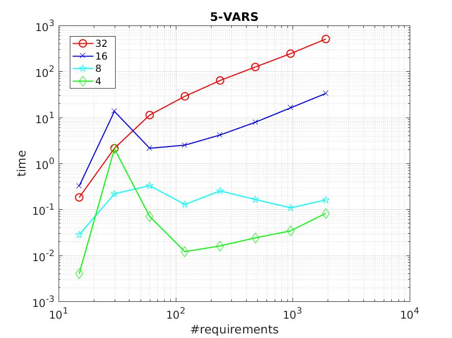
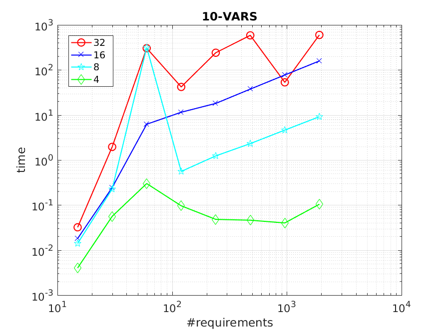
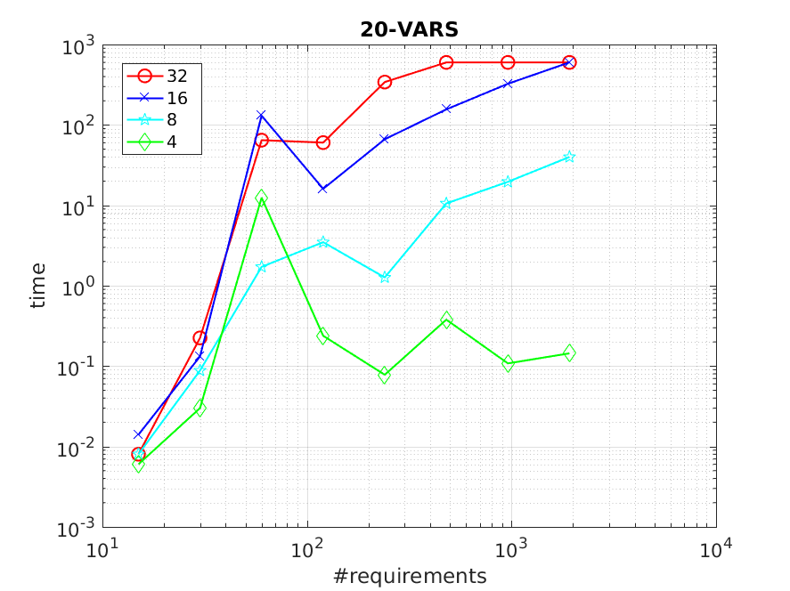
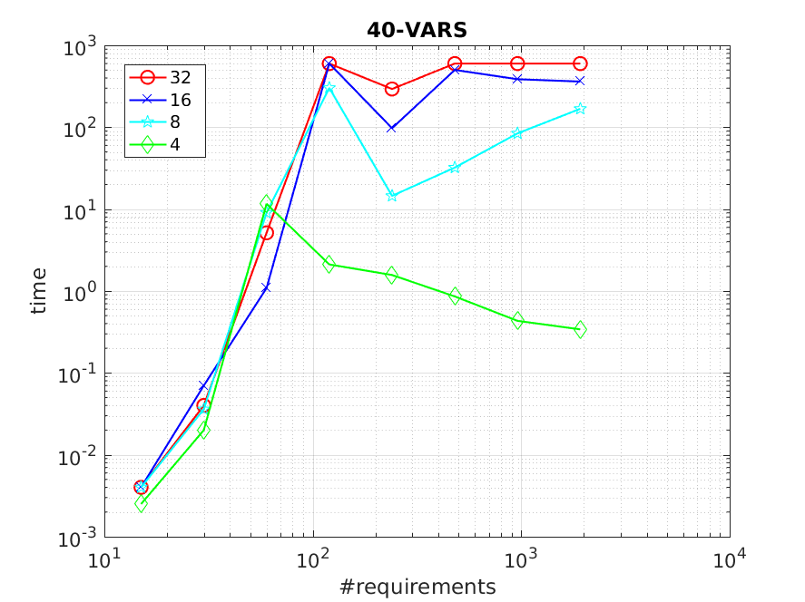
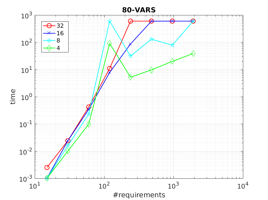
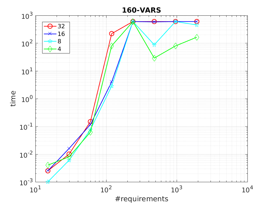
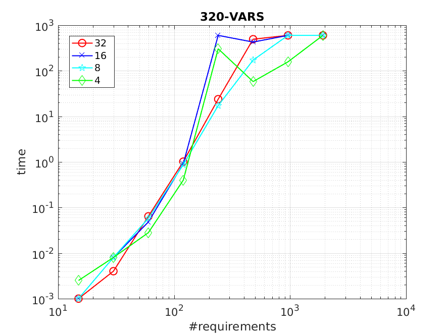
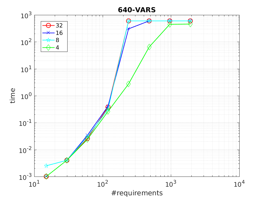
Figure 2: Scalability Analysis. On the $x$-axes ($y$-axes resp.) we report $\#req$ (CPU time in seconds resp.). Axis are both in logarithmic scale. In each plot we consider different values of $\#dom$. In particular, the diamond green line is for $\#dom$ = 4, the light blue line with stars is for $\#dom$ = 8, the blue crossed lines and red circled ones denote $\#dom=16$ and $\#dom=32$, respectively.

Evaluation of scalability.

The analysis involves 2560 different benchmarks generated as in the previous experiment. The initial value of $\#req$ has been set to 15, and it has been doubled until 1920, thus obtaining benchmarks with a total amount of requirements equals to 15, 30, 60, 120, 240, 480, 960, and 1920. Similarly has been done for $\#vars$ and $\#dom$; the former ranges from 5 to 640, while the latter ranges from 4 to 32. At the end of the generation, we obtained 10 different sets composed of 256 benchmarks. In Figure 2 we present the results, obtained running aalta. The Figure is composed by 8 plots, one for each value of $\#vars$. Looking at the plots in Figure 2, we can see that the difficulty of the problem increases when all the values of the considered parameters increase, and this is particularly true considering the total amount of requirements. The parameter $\#dom$ has a higher impact of difficulty when the number of variables is small. Indeed, when the number of variables is less then 40 there is a clear difference between solving time with $\#dom=4$ and $\#dom=32$. On the other hand when the number of variables increases, all the plots for various values of $\#dom$ are very close to each other. As a final remark, we can see that even considering the largest problem ($\#vars$ = 640, $\#dom$ = 32), more than the 60% of the problems are solved by aalta within the time limit of 10 minutes.

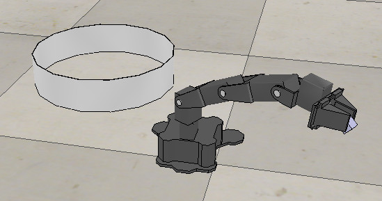
Figure 3: WidowX robotic arm moving a grabbed object in the bucket on the left.

5 Analysis with a Controller for a Robotic Manipulator

In this Section, as a basis for our experimental analysis, we consider a set of requirements from the design of an embedded controller for a robotic manipulator. The controller should direct a properly initialized robotic arm — and related vision system — to look for an object placed in a given position and move to such position in order to grab the object; once grabbed, the object is to be moved into a bucket placed in a given position and released without touching the bucket. The robot must stop even in the case of an unintended collision with other objects or with the robot itself — collisions can be detected using torque estimation from current sensors placed in the joints. Finally, if a general alarm is detected, e.g., by the interaction with a human supervisor, the robot must stop as soon as possible. The manipulator is a 4 degrees-of-freedom Trossen Robotics WidowX arm equipped with a gripper: Figure 3 shows a snapshot of the robot in the intended usage scenario taken from V-REP simulator. The design of the embedded controller is currently part of the activities related to the “Self-Healing System for Planetary Exploration” use case [16] in the context of the EU project CERBERO.

Pattern	Specification			Fault injections
	after	after_until	globally	after	after_until	globally
Absence	–	12	14	[F4]	–	[F3]
Existence	9	–	–	–	[F5]	[F4, F6]
Invariant	–	–	29	–	–	[F2, F6]
Precedence	–	–	1	–	–	–
ResponseChain	–	–	2	–	–	–
Response	1	–	4	–	–	[F1]
Universality	2	–	1	–	–	–

Table 2: Robotic use case requirements synopsis. The table is organized as follows: the first column reports the name of the patterns and it is followed by two groups of three columns denoted with the scope type: the first group refers to the intended specification, the second to the one with fault injections. Each cell in the first group reports the number of requirements grouped by pattern and by scope type. Cells in the second group categorize the 6 injected faults, labeled with F1, …, F6.

In this case study, constrained numerical signals are used to represent requirements related to various parameters, namely angle, speed, acceleration, and torque of the 4 joints, size of the object picked, and force exerted by the end-effector. We consider 75 requirements, including those involving scenario-independent constraints like joints limits, and mutual exclusion among states, as well as specific requirements related to the conditions to be met at each state. The set of requirements involved in our analysis includes 14 Boolean signals and 20 numerical ones. The full list of requirements is available at [17], each one of them expressed as a PSP($\mathcal{D}$). In Table 2 we present a synopsis of the requirements, to give an idea of the kind of patterns used in the specification.

Our first experiment is to run NuSMV-invar on the intended specification translated to LTL($\mathcal{D}_{C}$). The motivation for presenting the results with NuSMV-invar rather than aalta is twofold: While its performances are worse than aalta, NuSMV-invar is more robust in the sense that it either reaches the time limit or it solves the problem, without ever failing for unspecified reasons like aalta does at times; second, it turns out that NuSMV-invar can deal flawlessly and in reasonable CPU times with all the specifications we consider in this Section, both the intended one and the ones obtained by injecting faults. In particular, on the intended specification, NuSMV-invar is able to find a counterexample in 37.1 CPU seconds, meaning that there exists at least a model able to satisfy all the requirements simultaneously. Notice that the translation time from patterns to formulas in LTL($\mathcal{D}_{C}$) is negligible with respect to the solving time. Our second experiment is to run NuSMV-invar on the specification with some faults injected. In particular, we consider six different faults, and we extend the specification in six different ways considering one fault at a time. The patterns related to the faults are summarized in Table 2. Also in this case, we refer the reader to [17] for details. In case of faulty specifications, NuSMV-invar concludes that no counterexample exists, i..e, there is no model able to satisfy all the requirements simultaneously. In particular, in the case of F2 and F3, NuSMV-invar returned the result in 2.1 and 1.7 CPU seconds, respectively. Concerning the other faults, the tools was one order of magnitude slower in returning the satisfiability result. In particular, it spent 16.8, 50.4, 12.2, and 25.6 CPU seconds in the evaluation of the requirements when faults 1, 4, 5 and 6 are injected, respectively.

The noticeable difference in performances when checking for different faults in the specification is mainly due to the fact that F2 and F3 introduce an initial inconsistency, i.e., it would not be possible to initialize the system if they were present in the specification, whereas the remaining faults introduce inconsistencies related to interplay among constrains in time, and thus additional search is needed to spot problems. In order to explain this difference, let us first consider fault 2:

Globally, it is always the case that if state_init holds, then not arm_idle holds as well.

It turns out that in the intended specification there is one requirement specifying exactly the opposite, i.e., that when the robot is in state_init, then arm_idle must hold as well. Thus, the only models that satisfy both requirements are the ones preventing the robot arm to be in state_init. However, this is not possible because other requirements related to the state evolution of the system impose that state_init will eventually occur and, in particular, that it should be the first one. On the other hand, if we consider fault 6:

Globally, it is always the case that if arm_moving holds, then joint1_speed $>$ 15.5 holds as well.
Globally, arm_moving and proximity_sensor = 10.0 eventually holds.

we can see that the first requirement sets a lower speed bound at 15.5 $deg/s$ for joint1 when the arm is moving, while there exists a requirement in the intended specification setting an upper speed bound at 10 $deg/s$ when the proximity sensor detects an object closer than 20 $cm$. In this case, the model checker is still able to find a valid model in which proximity_sensor $<$ 20.0 never happens when arm_moving holds, but the second requirements in fault 6 prohibits this opportunity. It is exactly this kind of interplay among different temporal properties which makes NuSMV-invar slower in assessing the (in)consistency of some specifications.

6 Conclusions

Enabling the verification of high-level requirements is one of the key aspects towards the development of safety- and security-critical cyber-physical systems. Property Specification Patterns offer a viable path towards this target, but their expressiveness is often too restricted for practical applications. In this paper, we have extended basic PSPs over the constraint system $\mathcal{D}_{C}$, and we have provided an encoding from any PSP($\mathcal{D}_{C}$) into a corresponding LTL formula. This enables us to deal with many specifications of practical interest, and to verify them using automated reasoning systems currently available for LTL. Using realistically-sized specifications generated with an artificial probability model we have shown that our approach implemented on the tool aalta scales to problems containing more than a thousand requirements over hundreds of variables. Considering a real-world case study in the context of the EU project CERBERO, we have shown that it is feasible to check specifications and uncover injected faults, even without resorting to aalta, but considering the (slower, yet more robust) NuSMV. These results witness that our approach is viable and worth of adoption in the process of requirement engineering. Our next steps toward this goal will include easing the translation from natural language requirements to patterns, and extending the pattern language to deal with other relevant aspects of cyber-physical systems, e.g., real-time constraints.

Acknowledgments

The research of Luca Pulina and Simone Vuotto has been funded by the EU Commission’s H2020 Programme under grant agreement N. 732105 (CERBERO project).

References

- [1] Cimatti, A., Clarke, E., Giunchiglia, E., Giunchiglia, F., Pistore, M., Roveri, M., Sebastiani, R., Tacchella, A.: Nusmv 2: An opensource tool for symbolic model checking. In: International Conference on Computer Aided Verification. pp. 359–364. Springer (2002)
- [2] Clarke, E.M., Emerson, E.A., Sistla, A.P.: Automatic verification of finite-state concurrent systems using temporal logic specifications. ACM Transactions on Programming Languages and Systems (TOPLAS) 8(2), 244–263 (1986)
- [3] Comon, H., Cortier, V.: Flatness is not a weakness. In: Computer Science Logic. pp. 262–276. Springer (2000)
- [4] Demri, S., D’Souza, D.: An automata-theoretic approach to constraint LTL. In: FSTTCS. pp. 121–132. Springer (2002)
- [5] Dillon, L.K., Kutty, G., Moser, L.E., Melliar-Smith, P.M., Ramakrishna, Y.S.: A graphical interval logic for specifying concurrent systems. ACM Transactions on Software Engineering and Methodology (TOSEM) 3(2), 131–165 (1994)
- [6] Dokhanchi, A., Hoxha, B., Fainekos, G.: Metric interval temporal logic specification elicitation and debugging. In: . In 13. ACM IEEE International Conference on Formal Methods and Models for Codesign, MEMOCODE. pp. 21–23 (2015)
- [7] Dokhanchi, A., Hoxha, B., Fainekos, G.: Formal requirement debugging for testing and verification of cyber-physical systems. arXiv preprint arXiv:1607.02549 (2016)
- [8] Dwyer, M.B., Avrunin, G.S., Corbett, J.C.: Patterns in property specifications for finite-state verification. In: Software Engineering, 1999. Proceedings of the 1999 International Conference on. pp. 411–420. IEEE (1999)
- [9] Dwyer, M.B., Avrunin, G.S., Corbett, J.C., Halavi, H., Dillon, L., Corina, P.: Spec Patterns (1999), http://patterns.projects.cis.ksu.edu/, [Online; accessed 30-November-2017]
- [10] Hustadt, U., Konev, B.: TRP++ 2.0: A temporal resolution prover. In: CADE. vol. 2741, pp. 274–278. Springer (2003)
- [11] Konrad, S., Cheng, B.H.: Real-time specification patterns. In: Software engineering, 2005. icse 2005. proceedings. 27th international conference on. pp. 372–381. IEEE (2005)
- [12] Li, J., Pu, G., Zhang, L., Yao, Y., Vardi, M.Y., et al.: Polsat: A portfolio LTL satisfiability solver. arXiv preprint arXiv:1311.1602 (2013)
- [13] Li, J., Yao, Y., Pu, G., Zhang, L., He, J.: Aalta: an LTL satisfiability checker over infinite/finite traces. In: Proceedings of the 22nd ACM SIGSOFT International Symposium on Foundations of Software Engineering. pp. 731–734. ACM (2014)
- [14] Li, J., Zhang, L., Pu, G., Vardi, M.Y., He, J.: LTL satisfiability checking revisited. In: Temporal Representation and Reasoning (TIME), 2013 20th International Symposium on. pp. 91–98. IEEE (2013)
- [15] Lumpe, M., Meedeniya, I., Grunske, L.: PSPWizard: machine-assisted definition of temporal logical properties with specification patterns. In: Proceedings of the 19th ACM SIGSOFT symposium and the 13th European conference on Foundations of software engineering. pp. 468–471. ACM (2011)
- [16] Masin, M., Palumbo, F., Myrhaug, H., de Oliveira Filho, J., Pastena, M., Pelcat, M., Raffo, L., Regazzoni, F., Sanchez, A., Toffetti, A., et al.: Cross-layer design of reconfigurable cyber-physical systems. In: 2017 Design, Automation & Test in Europe Conference & Exhibition (DATE). pp. 740–745. IEEE (2017)
- [17] Narizzano, M., Pulina, L., Tacchella, A., Vuotto, S.: Robot Arm Usecase. https://github.com/SAGE-Lab/robot-arm-usecase (2017)
- [18] Pnueli, A.: The temporal logic of programs. In: Foundations of Computer Science, 1977., 18th Annual Symposium on. pp. 46–57. IEEE (1977)
- [19] Pnueli, A., Manna, Z.: The temporal logic of reactive and concurrent systems. Springer 16, 12 (1992)
- [20] Post, A., Hoenicke, J.: Formalization and analysis of real-time requirements: A feasibility study at bosch. Verified Software: Theories, Tools, Experiments pp. 225–240 (2012)
- [21] Rozier, K.Y.: PANDA (Portfolio Approach to Navigating the Design of Automata) (2011), https://ti.arc.nasa.gov/m/profile/kyrozier/PANDA/PANDA.html, [Online; accessed 23-January-2017]
- [22] Rozier, K.Y., Vardi, M.Y.: LTL satisfiability checking. In: Spin. vol. 4595, pp. 149–167. Springer (2007)
- [23] Rozier, K.Y., Vardi, M.Y.: LTL satisfiability checking. International Journal on Software Tools for Technology Transfer (STTT) 12(2), 123–137 (2010)
- [24] Rozier, K.Y., Vardi, M.Y.: A multi-encoding approach for LTL symbolic satisfiability checking. In: International Symposium on Formal Methods. pp. 417–431. Springer (2011)
- [25] Schwendimann, S.: A new one-pass tableau calculus for PLTL. In: International Conference on Automated Reasoning with Analytic Tableaux and Related Methods. pp. 277–291. Springer (1998)