Statistical sparsity
Abstract
The main contribution of this paper is a mathematical definition of statistical sparsity, which is expressed as a limiting property of a sequence of probability distributions. The limit is characterized by an exceedance measure and a rate parameter , both of which are unrelated to sample size. The definition is sufficient to encompass all sparsity models that have been suggested in the signal-detection literature. Sparsity implies that is small, and a sparse approximation is asymptotic in the rate parameter, typically with error in the sparse limit . To first order in sparsity, the sparse signal plus Gaussian noise convolution depends on the signal distribution only through its rate parameter and exceedance measure. This is one of several asymptotic approximations implied by the definition, each of which is most conveniently expressed in terms of the zeta-transformation of the exceedance measure. One implication is that two sparse families having the same exceedance measure are inferentially equivalent, and cannot be distinguished to first order. A converse implication for methodological strategy is that it may be more fruitful to focus on the exceedance measure, ignoring aspects of the signal distribution that have negligible effect on observables and on inferences. From this point of view, scale models and inverse-power measures seem particularly attractive.
Keywords: Convolution; Exceedance measure; False discovery; Infinite divisibility; Lévy measure; Post-selection inference; Signal activity; Tail inflation
1 Introduction
1.1 The role of a definition
Statistical sparsity is concerned partly with phenomena that are rare, partly with phenomena that are mostly zero, but more broadly with phenomena that are mostly negligible or seldom appreciably large. Progress in mathematics is seldom impeded by inadequacy of definitions, and the same may be said about progress in the development of sparsity as a concept in statistical work. But, sooner or later, definitions are needed in order to clarify ideas and to keep confusion at bay. The challenge is to formulate accurately a definition of sparsity that is faithful to current usage, and to explore its consequences. Our approach uses a probabilistic limit.
Statistical sparsity is defined in § 2 as a limiting property of a sequence of probability distributions that governs both the rate at which probability accumulates near the origin, and the rate at which it decreases elsewhere. Our definition covers all sparsity models that are found in the statistical literature on sparse-signal detection and estimation. It includes all two-group atom-and-slab mixtures, (Johnstone and Silverman 2004, Efron, 2009), all non-atomic spike-and-slab mixtures (George and McCulloch 1993; Rockova and George 2018), the low-index gamma model (Griffin and Brown, 2013), and many Gaussian scale mixtures such as the Cauchy scale family and the horseshoe scale family (Carvalho, Polson and Scott 2010).
The sparse limit is characterized by a rate parameter and a measure whose product determines the rarity of threshold exceedances. The exceedance measure is also the chief determinant of a certain restricted class of integrals, probabilities, and expected values that arise in probabilistic assessments of signal activity.
In many cases, a definition tells us only what is intuitively well known. But occasionally, a good mathematical definition reveals an aspect of the phenomenon that is unexpected and not readily apparent from a litany of examples. Sparsity is a case in point. The phenomenon may be intuitively obvious, but the definition in terms of a characteristic pair is much less so. The first reason for a definition is that it highlights the role of the characteristic pair and provides a definitive answer to the question of whether a particular probability model is or is not statistically sparse, in what way it deviates from sparsity, and so on.
The second reason is that the limit enables us to develop distributional approximations for inferential purposes in sparse signal-detection problems, i.e., approximations for the marginal distribution or the conditional distribution given the observation. The sequence is essential because a sparse approximation is asymptotic in the rate parameter , and is unrelated to sample size and sample configuration.
The third reason is that, while the sequence of distributions determines the exceedance measure, the exceedance measure does not determine the distributions. Two sequences having the same exceedance measure are first-order equivalent in the sense that all marginal and conditional distributions depend only on the exceedance measure. For example, to certain atom-free spike-and-slab mixtures there corresponds an equivalent atom-and-slab mixture. Likewise, the Cauchy and horseshoe scale families are equivalent, but they are not equivalent to the low-index gamma model.
1.2 Statistical implications
The novelty of this paper lies entirely in the definition of sparsity, which is statistically interesting on account of its implications. We leave it to the reader to decide whether the implications described in §§ 3–6 are useful or relevant or have practical consequences, but utility and practical considerations play no role in their derivation. The over-riding implication is that it is futile to estimate any functional of the signal distribution that is not first-order identifiable from the data that are observed. Subsidiary implications flowing from the definition are as follows:
-
•
the use of in place of the signal distribution for model specification;
-
•
the role of the asymptotic likelihood for parameter estimation (§§ 3.4, 7);
-
•
the role of the zeta function for inference about the signal given the data (§ 5);
-
•
the connection between scale models and inverse-power measures (§ 4);
-
•
the interpretation of the Benjamini-Hochberg procedure in terms of conditional exceedance rather than conditional false discovery or null signals (§ 5.4).
The zeta transformation is defined in § 3; it plays a key role for inference in the standard sparse signal detection model. Section 4 focuses on the inverse-power exceedance measures, a class that includes the sparse Cauchy model, the horseshoe model and all other scale families having similar tail behaviour. Within the inverse-power class, there exists a particular family of probability distributions, called the -scale family, that has a highly unusual but extremely useful property. Every Gaussian- convolution that arises in the signal-plus-noise model is expressible exactly as a binary Gaussian- mixture. This is a closure or self-conjugacy property, which means that the observation distribution belongs to the same family as the signal.
Section 5 shows how the zeta function determines the asymptotic conditional distribution of the signal given the observation, and Tweedie’s formula for the conditional moment generating function. The conditional activity, or -exceedance probability, is shown to be a rational function of the zeta transformation, which is closely related to the Benjamini-Hochberg procedure (Benjamini and Hochberg 1995).
2 Sparse limit: definitions
2.1 Exceedance measure
The sparse limit involves an exceedance measure, which is defined as follows.
Definition 1.
A non-negative measure on the real line excluding the origin is termed an exceedance measure if . A measure satisfying is called a unit exceedance measure.
Although the motivation for this definition is unconnected with stochastic processes, every exceedance measure is the Lévy measure of an infinitely divisible distribution on the real line, and vice-versa. No constraint is imposed on the total measure, which may be finite or infinite.
To every non-zero exceedance measure there corresponds a ray of proportional measures. Each ray contains as a reference point a unit measure such that is a probability distribution on . For example, the unit inverse-power measures are
| (1) |
for .
Definition 2.
The activity index gauges the behaviour in a neighbourhood of the origin:
Every finite measure has activity index zero; the measure (1) has activity index .
Comment 1: The activity index is strictly less than two because continuity of for implies that is an open set containing 2. In particular, the limit arises in § 3.5.
Definition 3.
The space of Lévy-integrable functions consists of bounded continuous functions on the real line such that is also bounded and continuous. Lévy integrability implies for every and every exceedance measure .
The functions , and belong to .
2.2 Sparse limit
Let be a sequence of probability distributions indexed by , and converging weakly to the Dirac measure as . Sparsity is a rate condition governing the approach to the weak limit.
Definition 4.
A sequence of probability distributions is said to have a sparse limit with rate if there exists a unit exceedance measure such that
| (2) |
for every . Otherwise, if the limit is zero for every , the sequence is said to be sparse with rate .
The motivation for this definition comes from extreme-value theory, which focuses on exceedances over high thresholds (Davison and Smith 1990). Each sparse-signal threshold is fixed as , but is automatically high relative to the bulk of the distribution: in this respect, the parallel with extreme-value theory is close. Unlike extreme-value theory, sparsity places no emphasis on limit distributions for the excesses over any threshold. Formally setting equal to the indicator function for the event or in the integrals (2) gives the motivating condition—that the sparsity rate is the rarity of exceedances
| (3) |
There is a similar limit for negative exceedances, and any other subset whose closure does not include zero.
Comment 2: The integral definition implies (3), but the converse fails if the limit in (3) is not a Lévy measure. For example, the Dirac-Gaussian mixture does not have a sparse limit, but (3) is satisfied by with . Section 6 discusses another example where the limit measure is non-trivial but not in the Lévy class.
Since the definition involves only the limit , it is always possible to re-parameterize by the rate function, so that . This standard parameterization is assumed where it is convenient.
Definition 5.
Sparse-limit equivalence: Regardless of their parameterization, two sparse families having the same exceedance measure are said to be equivalent in the sparse limit.
Let and be two families having the same unit exceedance measure , both taken in the standard parameterization with rate parameter . In effect, the rate parameterization matches each distribution in one family with a sparsity-matching distribution in the other, so the families are in 1–1 correspondence, at least in the approach to the limit. For any function , the limit integrals are finite and equal:
Consequently, near the sparse limit, both integrals may be approximated by
This analysis implies that every -integral using as the signal distribution is effectively the same as the integral using at the corresponding sparsity level.
Definition 6.
Sparse scale family: A scale family of distributions with density is called a sparse scale family if it is sparse in the small-scale limit . The rate function need not coincide with the scale parameter.
The Student- scale family on degrees of freedom is a sparse scale family with rate function and exceedance density proportional to .
If the scale family is sparse with rate parameter , then, for small ,
Setting and gives as . Conversely, for , implying that for some power . If is not symmetric, the power index for may be a different number. It follows that the exceedance density of a sparse scale family is an inverse power function , the same as the tail behaviour of as .
2.3 Infinite divisibility
Let be an infinitely divisible probability distribution on the real line, and let be the Lévy family indexed by the convolution parameter, i.e., with . The Lévy process is sparse with rate , and the exceedance measure is the Lévy measure (Barndorff-Nielsen and Hubalek, 2008).
To each exceedance measure there corresponds an infinite equivalence class of sparse sequences, most of which are not closed under convolution. This result tells us that each equivalence class contains exactly one Lévy process; the zero equivalence class contains the Gaussian family, i.e., the Brownian motion process. Despite this characterization, exceedance measures and Lévy processes have not played a prominent role in either frequentist or non-frequentist work on sparsity.
Comment 3: A typical spike-and-slab distribution is not infinitely divisible. However, there are exceptions. For each positive pair , the atom-and-slab lasso distribution
is infinitely divisible with finite Lévy measure
| (4) |
For each , the family exists, but the distributions are not easily exhibited.
The atom-and-slab lasso family with as the sparsity rate parameter is not to be confused with the Lévy family in which is held fixed. The exceedance measures are and .
2.4 Sparsity expansion
Weak convergence of the sequence to the Dirac measure is concerned with the behaviour of -integrals for a suitable class of functions. For any bounded continuous function having one continuous derivative at zero, the symmetrized function
is near the origin. Thus is Lévy integrable and, if is symmetric, sparseness implies a linear expansion for small :
The exceedance measure is the directional derivative or linear operator governing the approach to the weak limit:
in the sense of integrals. Sparsity determines the difference , but only to first order in .
2.5 Examples
For , the exceedance event , or activity event, is the complement of the closed interval .
Example 1: The -exceedance probability for the Laplace distribution with density is , implying for every and . The scale family is sparse with rate for every . There is no definite sparsity rate parameter satisfying (2) with a finite non-zero limit, so we say that the sequence belongs to the zero-activity class. The Gaussian scale family, and all other scale families having exponential tails, have the same property. So far as this paper is concerned all sparse families in this class are trivial and equivalent.
Example 2: Let be a probability distribution on the real line. The atom and slab family indexed by is sparse with exceedance measure proportional to . The unit exceedance measure is , where , and the exceedance rate is , so the product satisfies . The activity-reduction factors for the standard Laplace, Cauchy and Gaussian distributions are , and respectively.
The mixture-indexed spike and -slab family with a fixed scale parameter belongs to the finite class; it is not to be confused with the atom-free -scale family or intermediate combinations.
Example 3a: The family of double gamma distributions with density
is sparse with rate parameter and exceedance density . The total mass is infinite but there is no atom at zero.
Example 3b: For fixed , the re-scaled double gamma family with density is sparse with rate parameter and exceedance density , which depends on . Each of the sub-families for different has its own exceedance measure. These are not equivalent because they are not proportional.
For fixed index , the double gamma scale family is also sparse with rate for every , so the scale family belongs to the zero-activity class.
Example 4: The Cauchy family with probable error and density
is sparse with inverse-square exceedance and rate . The scale families
have the same rate parameter and exceedance measure. Similar remarks apply to a large number of families that have been proposed as prior distributions in the literature, including the scale family generated by various Gaussian mixtures such as the horseshoe distribution with density .
Example 5a: Consider the distribution with density
and let be the density of the re-scaled distribution. Then the family is sparse with rate parameter and inverse-square exceedance.
Example 5b: For , let , and let
This scale family is sparse with the same rate function and inverse-square exceedance measure as the previous two. The weight function has no role in the limit provided that the integral is finite, for small , and as .
Example 6: The Dirac-Gaussian mixture converges to a point mass, as does , but neither mixture has a sparse limit according to the definition. The Dirac-Cauchy mixture has a sparse inverse-square limit with rate parameter , but does not.
3 Zeta function and zeta measure
3.1 Definitions
We assume henceforth that every sparse family is symmetric, and the exceedance measure is expressed in unit form, so that .
To each exceedance measure there corresponds a zeta function
| (5) |
which is positive and finite, symmetric and convex, satisfying . By construction, the zeta function is the cumulant function of the infinitely divisible distribution with down-weighted Lévy measure . The zeta function is analytic at the origin, so this Lévy process has finite moments of all orders.
Numerical values are shown in Table 1 for three inverse-power measures.
The zeta measure is the integrand in (5):
| (6) |
which is a weighted linear combination of symmetric measures with coefficients for , and finite total mass . The zeta measure occurs as one of two components of the conditional distribution in § 5.3.
| Table 1: Zeta function for three inverse-power exceedance measures. | |||||||||||||
|---|---|---|---|---|---|---|---|---|---|---|---|---|---|
| 2.0 | 2.2 | 2.4 | 2.6 | 2.8 | 3.0 | 3.2 | 3.4 | 3.6 | 3.8 | 4.0 | 4.2 | 4.4 | |
| 0.5 | 1.9 | 2.7 | 3.9 | 5.8 | 8.8 | 13.9 | 22.9 | 39.4 | 70.9 | 133.7 | 264.3 | 547.6 | 1188.4 |
| 1.0 | 3.1 | 4.2 | 5.8 | 8.1 | 11.6 | 17.2 | 26.5 | 42.7 | 72.5 | 129.6 | 244.2 | 485.0 | 1013.9 |
| 1.5 | 3.8 | 4.8 | 6.2 | 8.1 | 10.7 | 14.4 | 20.2 | 29.5 | 45.5 | 74.4 | 129.8 | 241.6 | 478.7 |
3.2 Tail inflation factor
The zeta function is an integral transformation much like a Laplace transform, i.e., formally is a measure on the observation space and is a function on the dual space. However, if is the standard normal density, the product is also a probability density with characteristic function
| (7) | |||||
Provided that is a unit exceedance measure, the value at is one.
Section 3.4 shows that is the tail-inflation component of the marginal distribution of the observations. The left panel of Figure 1 shows the density function for the inverse-power exceedance measures, all of which have similar bimodal distributions differing chiefly in modal height and tail behaviour. There is a certain qualitative similarity with a pair of distributions depicted in Figure 1 of Johnson and Rossell (2009), and recommended there as priors for testing a Gaussian mean.
For typical exceedance measures having regularly-varying tails, the characteristic function of is not analytic at the origin, in which case the distribution does not have finite moments. For example, if is the inverse-power exceedance (1) for some , the characteristic function (7) reduces to
| (8) |
where . By contrast, if has exponential tails, the integral in (7) is
which is analytic at the origin. A derivation is sketched near the end of § 4.2.
3.3 Sparsity integrals
To see how the zeta function arises in sparsity calculations, consider first the integral of the weighted distribution
where is the rate function. Second, for any sparse family, the Laplace transform is
The normalized family is sparse with rate , exceedance measure , and Laplace transform .
3.4 Signal plus noise convolution
Suppose that the observation is a sum of two independent unobserved random variables , where the signal is sparse, and is a standard Gaussian variable. Then the joint density of at is , while the marginal density of the observation is a Gaussian- mixture:
| (9) | |||||
For every sparse family, the sparsity parameter satisfies , which provides a recipe for consistent estimation. Alternatively, if , or are given, the mixture (9) can be fitted directly by maximum likelihood: see § 7.
Comment 4: The Gaussian- mixture is a consequence of sparsity alone. It is compatible with a sparse atom-and-slab mixture for signals, but the sparsity rate is strictly less than the slab weight . The identity implies that cannot be the response distribution for any signal subset, so the sparsity rate in the marginal mixture (9) is not interpretable as the prior probability of a non-null signal in the standard two-group model (Johnstone and Silverman, 2004; Efron, 2008, 2010).
Although determines the marginal density to first order, Example 4 in § 2.5 show that does not determine the null fraction , which may be zero.


3.5 Two inequalities
For fixed , the zeta function is linear in , so the maximum necessarily occurs on the boundary at an atomic measure for some , or, if the maximum does not exist, the supremum occurs in the limit . For , the limit point prevails, and the supremum is
which is attained in the limit for the inverse-power class. Accordingly, the leading Taylor coefficient satisfies .
The second inequality is concerned with the behaviour of the zeta measure in a neighbourhood of the origin. If has an atom at , then also has an atom at . But implies that there is no atom at the origin, i.e., for each
| (10) |
It follows that the density limit is zero for low-activity measures and infinite for : see Fig. 3.
For , the series expansion with positive coefficients implies
For every and , it follows that
| (11) | |||||
For example, implies .
4 Inverse power exceedances
4.1 Summary
This section summarizes, without proofs, the role of the zeta function (5) for sparse scale families whose unit exceedance densities for are shown in (1). It has the following properties.
-
1.
The zeta function is expressible as a power series
(12) which is symmetric with infinite radius of convergence.
-
2.
The characteristic function of is , where is given in (8).
-
3.
The scale family is sparse with rate parameter and the same exceedance density (1).
-
4.
Let and be independent. To each pair of coefficients with there corresponds a number such that the linear combination is distributed as the mixture .
-
5.
The marginal distribution of is a mixture .
The statement in 5 is a little imprecise because the signal distribution is not mentioned. Modulo the scale factor that occurs implicitly in 4, the statement is exact if the signal is distributed as for arbitrary , which determines the mixture weight . It is also correct, modulo a similar scale factor, if the signal is distributed according to the mixture itself. More importantly, it is correct for every signal distribution in this inverse-power equivalence class, but with error in the approach to the sparse limit.
4.2 The convolution-mixture theorem
With defined by its series expansion (12), the probability distribution with density
has a remarkable property that makes it singularly well adapted for statistical applications related to sparse signals contaminated with additive Gaussian error. Not only is the -scale family sparse with inverse-power exceedance measure, but each Gaussian- convolution is also expressible as a binary Gaussian- mixture as follows.
Theorem 7.
Convolution-mixture: For arbitrary scalars , let
where and are independent random variables. Also, let be the mixture
Then and have the same distribution denoted by .
The theorem states that every linear combination with norm is equal in distribution to an equi-norm Gaussian- mixture. An arbitrary binary mixture is not expressible as a convolution unless the two scale parameters are equal.
Proof.
There is an extension to any exceedance measure that is an inverse-power mixture.
4.3 Identifiability
The convolution-mixture theorem asserts that
| (13) |
where . Of the four parameters , only three are identifiable in the marginal distribution. In principle, lack of identifiability is a serious inferential obstacle because the conditional distribution of the signal given depends on all four parameters. The difficulty is resolved in this paper, as it is elsewhere in the literature, by fixing . Without such an assumption, there are severe limitations to what can be learned from the data about the signal.
5 Conditional distribution
5.1 Tweedie’s formula
Provided that the error distribution is standard Gaussian, the argument used in § 3.4 shows that the moment generating function of the conditional distribution of the signal given is
| (14) |
depending, to first order in , only on the zeta function of the exceedance measure. In particular, the th conditional moment is , which is the first-order asymptotic version of Tweedie’s formula (Efron, 2011). For the inverse-square exceedance, the conditional mean is depicted in the middle panel of Figure 1 for a range of sparsity levels.
5.2 Mixture interpretation
Let be the probability distribution whose moment generating function is , i.e., (14) with and , and let be the exponentially tilted distribution whose moment generating function is , i.e., (14) with . Then, the two-component mixture
| (15) |
has moment generating function (14). Holding fixed as , this heuristic argument suggests that the asymptotic conditional distribution of the signal is a specific two-component mixture in which the th moment of is . The argument is non-rigorous because there is no limit distribution ( for fixed implies and ), but the moment-matching intuition is essentially correct. However, the Dirac atom in (15) could be replaced by with no first-order effect on the generating function, so, (14) does not imply that the conditional distribution has an atom at zero.
For the inverse-power family, the Laplace integral approximation for large is
implying that is approximately Gaussian with mean and unit variance. Asymptotically, for fixed implies , so the two components in (15) are asymptotically well separated with negligible probability assigned to bounded intervals for which . This behaviour is typical for exceedance measures whose log density is slowly varying at infinity, but it is not universal. Bounded and discrete exceedance measures exhibit very different behaviours.
5.3 Symmetrization
The conditional density of the signal given is proportional to the joint density,
and the symmetrized conditional distribution is proportional to
The latter approximation is understood in the usual sense of integrals.
The ratio of the conditional density at to that at is , so the conditional density may be recovered from the symmetrized version by multiplication by the bias function . Without loss of generality, therefore, we focus on the sparse limit of the symmetrized distribution shown above, ignoring terms of order .
To first order, the symmetrized conditional distribution is a mixture consisting of two components:
-
1.
A central spike distribution with weight proportional to ;
-
2.
The zeta distribution with weight proportional to .
The moment-generating function of the central spike is , and the normalization constant for the mixture is the total weight .
For , the inequality (see § 3.5) implies that the net weight on the central spike is at least . In other words, for typical -values less than 5%, and , the central spike is the dominant feature of the conditional distribution.
If , the zeta density has an integrable singularity at the origin. Ordinarily, this spike is not visible because it overlaps the central spike and its relative weight is small. But there are exceptions in which the central spike has zero density at the origin. See Fig. 3 in § 7 for one illustration.
5.4 Signal activity probability
The conditional distribution given is symmetric with sparse-limit distribution
which is negligibly different from . For any symmetric event such as whose closure does not include zero, the first-order conditional probability given is the weighted linear combination
Since , and (10) implies that tends to zero for low thresholds, the asymptotic low-threshold activity bound for fixed is
| (16) |
The argument for (16) or its complement as an asymptotic approximation with negligible asymptotic error is more delicate than that for the inequality. First, the approximation requires as , which implies a lower bound on the activity threshold. Second, for at a rate such that is bounded below, the approximation also requires . Ordinarily, if has unbounded support, increases super-linearly, i.e., , in which case the condition that be bounded below implies for every . Consequently, for every fixed threshold , the inequality (11) implies
Super-linearity implies that the ratio tends to zero as . The zero-order conditional non-exceedance probability is then
which is independent of . The non-exceedance probability serves as an upper bound for the local false-positive rate,
| (17) |
5.5 Tail average activity
Multiplication of (17) by the marginal density, and integration over gives the tail-average -inactivity probability
| (18) |
For bounded and every fixed threshold , this ratio of tail integrals is a re-interpretation of the Benjamini-Hochberg procedure, which determines the data threshold corresponding to any specified tail-average inactivity rate. The B-H procedure controls the tail-average false-positive rate in the sense that the threshold satisfying (18) serves as an upper bound. It does not approximate the tail-average false-positive rate or the local false-positive rate, both of which depend crucially on the null atom , which could be zero.
6 Hyperactivity
6.1 The Student scale family
Student’s scale family of signal distributions satisfies
for , so the limit measure exists with rate . Unfortunately this limit is not a Lévy measure, so definition (2) is not satisfied, and the approximations developed in the preceding sections do not apply. For example, if or , the integral behaves as , i.e., , not .
The -scale family is an instance of a first-order hyperactive model for which the exceedance measure exists and is -integrable. First-order hyperactivity typically implies that the exceedance density near the origin is for some . The next section provides a sketch of the modifications needed to accommodate such behaviour.
6.2 Hyperactivity integrals
Let be a first-order hyperactive exceedance measure, i.e., is a non-zero symmetric Lévy measure. Among the positive multiples of , the natural reference point satisfies
| (19) |
For the model, the unit inverse quartic exceedance density is .
The first-order asymptotic theory for hyperactive sparse models is determined by the exceedance measure plus two rate parameters as follows:
for bounded continuous Lévy-integrable functions . The rate parameters for the -scale model are and , both tending to zero as , but not at the same rate.
To first order in sparsity,
implying that .
To ensure integrability at the origin, the definition of the zeta function is modified to
implying that near the origin. Provided that satisfies (19), the product is a probability density function. Its characteristic function is
which simplifies to for the inverse quartic.
The marginal distribution of for a first-order hyperactive sparse model is a three-component mixture of the density functions , and :
Note that the basis distributions are fixed, while the coefficients are sparsity-dependent. The chief consequence of signal hyperactivity is that the non-Gaussian perturbations are not of equal order in sparsity: asymptotically, . If it is convenient, the first two components may be combined so that
at the cost of a small increase in the variance of the Gaussian component.
All of the results in §§ 3 and 4 may be extended to hyperactive models with replaced by . Tweedie’s formula for the conditional mean of the signal involves both rate parameters:
7 Illustration
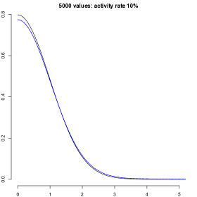
The left panel of Figure 2 shows a histogram of the absolute values of 5000 independent responses generated by Efron’s (2011) version of the sparse signal plus Gaussian noise model
where the s are independent random variables, and the signals are
for , and otherwise. The absolute non-zero signals are approximately exponentially distributed, and the mixture fraction is 10%. But a substantial fraction of the signals are small, and consequently undetectable in the presence of additive standard Gaussian noise. Example 2 in § 2.5 implies that the effective mixture fraction is
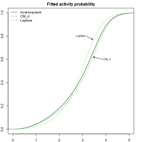
The developments in this paper suggest two ways to proceed, both using the inverse-power family of exceedance measures for illustration. The first is to estimate the parameter by maximizing the asymptotic log likelihood
Maximization with no constraints on gives , , and relative to the value at . The solid line in Fig 2b shows the fitted conditional activity probability as a function of .
The preferred option is to include a free scale parameter, , and to estimate subject to the condition as implied by the convolution-mixture (13). The log likelihood function for the model is
Constrained maximization gives
on the boundary at , for a maximum of 122.95 relative to .
For the marginal distribution of absolute values, the table below compares five quantiles of the Laplace-Gaussian mixture with the corresponding quantiles of the fitted distribution:
The match is reasonably satisfactory at least up to the 99.5 percentile. Only at the most extreme quantiles does the difference between the exponential tail of the L-G mixture and the inverse-power tail of the mixture become apparent. This discrepancy could be viewed as a deficiency of the class of inverse-power measures, but we are more inclined to view it as a deficiency of the Laplacian model for signals.
The dashed line in Fig 2b shows the fitted conditional activity probability as a function of . The difference between the two activity curves is small, and is due partly to the re-scaling () that occurs in the fit, and partly to the small difference in fitted rates. For example, the fitted conditional activity probabilities given are 46.3% and 42.9% respectively.
For this example, we know that the signals were effectively generated using the short-tailed atom-and-slab Laplace model, which is associated with the two-parameter Lévy measure in (4) with and . Using the associated zeta function, the asymptotic log likelihood achieves a maximum of 135.3 at , . In this setting, is the Lévy convolution parameter, and the likelihood function is essentially constant in over the range . For , the marginal density (9) covers both atomic and non-atomic spike-and-slab Laplace models such as , and the log likelihood is the same for all models in this equivalence class. The Laplace-activity curve shown in Fig. 2b also applies in the non-atomic setting, with the threshold-exceedance interpretation (17).
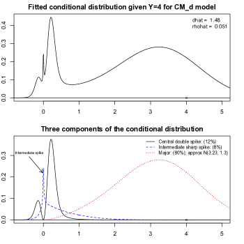
In the model, implies that the fitted conditional density given has a -singularity at the origin, which is clearly visible for in Fig. 3a. Figure 3b shows the additive decomposition of the conditional density in which the central double spike has net weight 12%, and the zeta component has weight 88%. The zeta-measure is decomposed further as a two-part mixture along the lines of § 6. The intermediate spike has density and weight proportional to , which is asymptotically negligible compared with , but not numerically negligible for . The remaining major component is unimodal with density
and weight proportional to . The latter can be approximated with reasonable accuracy by a Gaussian distribution.
The asymptotic theory in this paper tells us that, if is small, every model in the inverse-power class, such as the sparse Student , must produce essentially the same fit, with similar estimates for . In all cases, the conditional distribution given has a two-part decomposition as described in § 5.3. The asymptotic theory says little about the appearance of the central spike other than its total mass and the fact that it is concentrated near the origin. The central spike is bimodal for the model but unimodal for the sparse Student and most atom-free spike-and-slab mixtures. In neither case could the conditional distribution be said to have an atom at zero. But the asymptotic theory also tells us that the zeta component depends only on the exceedance measure, so the zeta measure, and its two-part decomposition in Figure 3, are the same for all models in the same sparsity class. To that extent at least, only the exceedance measure matters. There are indications that a second-order analysis might be capable of offering a more detailed description of the behaviour of the conditional distribution in the neighbourhood of the origin, but this paper stops at first order.
8 Acknowledgements
We are grateful to Jiyi Liu for pointing out that the convolution-mixture property in section 4.2 implies a certain form for the characteristic function, and ultimately for supplying a proof that the characteristic function of has this form.
9 References
Barndorff-Nielsen, O.E. and Hubalek, F. (2008) Probability measures, Lévy measures and analyticity in time. Bernoulli 14, 764–790.
Benjamini, Y., and Hochberg, Y. (1995). Controlling the false discovery rate: A practical and powerful approach to multiple testing. J. Roy. Statist. Soc. B, 57, 289-300
Carvalho, C.M., Polson, N.G. and Scott, J.G. (2010) The horseshoe estimator for sparse signals. Biometrika 97, 465–480.
Davison, A.C. and Smith, R.L. (1990) Models for exceedances over high thresholds. J. Roy. Statist. Soc. B 52, 393–442.
Efron, B. (2008) Microarrays, empirical Bayes and the two-groups model. Statist. Sci. 23, 1–22.
Efron, B. (2009) Empirical Bayes estimates for large-scale prediction problems. Journal of the American Statistical Association, 104, 1015–1028.
Efron, B. (2010) Large-Scale Inference: Empirical Bayes Methods for Estimation, Testing and Prediction. Cambridge University Press.
Efron, B. (2011) Tweedie’s formula and selection bias. Journal of the American Statistical Association, 106, 1602–1614.
George, E.I. and McCulloch, R.E. (1993) Variable selection via Gibbs sampling. J. Amer. Statist. Assoc., 88, 881–889.
Griffin, J.E. and Brown, P.E. (2013) Some priors for sparse regression modelling. Bayesian Analysis 8, 691–702.
Johnstone, I. and Silverman, B.W. (2004) Needles and straw in haystacks: Empirical-Bayes estimates of possibly sparse sequences. The Annals of Statistics, 32, 1594–1649.
Johnson, V.E. and Rossell, D. (2010) On the use of non-local prior densities in Bayesian hypothesis tests. J. Roy. Statist. Soc. B 72, 143–170.
Rockova, V. and George, E.I. (2018) The spike and slab LASSO. Journal of the American Statistical Association (to appear). https://doi.org/10.1080/01621459.2016.1260469