A semi-implicit scheme based on Arrow-Hurwicz method for saddle point problems

Abstract

We search saddle points for a large class of convex-concave Lagrangian. A generalized explicit iterative scheme based on Arrow-Hurwicz method converges to a saddle point of the problem. We also propose in this work, a convergent semi-implicit scheme in order to accelerate the convergence of the iterative process. Numerical experiments are provided for a nontrivial numerical problem modeling an optimal shape problem of thin torsion rods [1]. This semi-implicit scheme is figured out in practice robustly efficient in comparison with the explicit one.

49M29, 65B99, 65K05.

1 Introduction

In calculus of variations, we usually deal with problems of the following kind

$({𝒫}_h)$ $$\inf_{u\in C}\int_{\Omega}[\varphi(\nabla u)+h(u)]\,dx$$

where $\Omega$ is an open bounded subset of $\mathbb{R}^{N}$, the constraint is given by

$$C=\left\{u\in W^{1,p}(\Omega),u=u_{0}\text{\; on \;}\partial\Omega\right\},$$

and functions $\varphi:\mathbb{R}^{N}\to\mathbb{R}$ and $h:\mathbb{R}\to\mathbb{R}$ are convex continuous. The integrands satisfy suitable growth conditions to ensure the well-posedness of the problem.

Let us consider for instance a problem arising in shape optimization of thin torsion rods [1] to be a prototype situation

$$m(s):=\inf\left\{\int_{\Omega}\varphi(\nabla u):u\in H^{1}_{0}(\Omega),\int_{\Omega}u=s\right\}$$

with $N=2$ and $\varphi$ being a convex function given by

$$\varphi(z):=\begin{cases}\frac{1}{2}(|z|^{2}+1)&\text{\; if \;}|z|\geq 1\\ |z|&\text{\; if \;}|z|\leq 1.\end{cases}$$

This is a convex problem without presence of $h$. Moreover, $\varphi$ is not differentiable at the origin.

By duality argument, we can rewrite problem $(\mathcal{P}_{h})$ as a saddle point problem

$({ℳ}_h)$ $$\inf_{u\in C}\sup_{p\in K}\int_{\Omega}[\nabla u\cdot p+h(u)-\varphi^{*}(p)]dx$$

with $K=L^{p^{\prime}}(\Omega;\mathbb{R}^{N})$ and $\varphi^{*}$ being the Fenchel conjugate of $\varphi$ [9]. We denote by $L(u,p)$ the Lagrangian

$$L(u,p)=\int_{\Omega}[\nabla u\cdot p+h(u)-\varphi^{*}(p)]dx.$$

Our aim is to find solutions of $(\mathcal{P}_{h})$ by means of the saddle point problem $(\mathcal{M}_{h})$. We recall that a saddle point $(\hat{u},\hat{p})$ of $L(u,p)$ in $C\times K$ is characterized by the inequalities

(1) $$L(\hat{u},p)\leq L(\hat{u},\hat{p})\leq L(u,\hat{p}),\ \forall u\in C,\ \forall p\in K.$$

Usually, we immediately think of the gradient descent-ascent so as to seek a saddle point. For a general Lagrangian $L(u,p)$, the simplest approach introduced by Arrow and Hurwicz has the form

$$p_{n+1}=\Pi_{K}\Big{(}p_{n}+\tau_{n}\frac{\partial L}{\partial p}(u_{n},p_{n})\Big{)}$$

$$u_{n+1}=\Pi_{C}\Big{(}u_{n}-\tau_{n}\frac{\partial L}{\partial u}(u_{n},p_{n})\Big{)}.$$

where $\Pi_{K},\Pi_{C}$ are orthogonal projections on the closed convex sets $K$ and $C$, respectively. However, this first-order iterative optimization algorithm converges under very stringent conditions (like strict convexity-concavity) and special choosing of stepsizes $\tau_{n}\to 0,\;\sum_{n=0}^{\infty}\tau_{n}=\infty$ [11]. To overcome these difficulties, L. D. Popov [15] gave a modification of the Arrow-Hurwicz method by introducing the so-called "leading" point, denoted by $(\overline{u}_{n},\overline{p}_{n})$, which is an auxiliary point in order to jump to the next approximation with the help of the gradient direction,

$$p_{n+1}=\Pi_{K}\Big{(}p_{n}+\tau\frac{\partial L}{\partial p}(\overline{u}_{n},\overline{p}_{n})\Big{)}$$

$$u_{n+1}=\Pi_{C}\Big{(}u_{n}-\tau\frac{\partial L}{\partial u}(\overline{u}_{n},\overline{p}_{n})\Big{)}$$

$$\overline{p}_{n+1}=\Pi_{K}\Big{(}p_{n+1}+\tau\frac{\partial L}{\partial p}(\overline{u}_{n},\overline{p}_{n})\Big{)}$$

$$\overline{u}_{n+1}=\Pi_{C}\Big{(}u_{n+1}-\tau\frac{\partial L}{\partial u}(\overline{u}_{n},\overline{p}_{n})\Big{)}.$$

In his paper, he proved that there exists a positive scalar $\tau_{0}$ such that the modified algorithm converges for all constant stepsize $\tau$ taken in the interval $0<\tau<\tau_{0}$. This improvement enlarges the class of applicable problems whose convex-concave Lagrangians have derivatives satisfying Lipschitz conditions. It is clear that leading points makes the iterative processes more stable. But, because of extra projections, the more complicated the projections are, the heavier computation is. So, in some cases, replacing the extra projections as well as leading points is necessary. Chambolle-Pock et al. [14, 7] started dealing with a typical Lagrangian which is a linear form

$$L(u,p)=\langle Au,p\rangle+\langle f,u\rangle-\langle g,p\rangle,$$

where $A$ is a bounded linear operator and $\langle\cdot,\cdot\rangle$ denotes the associated scalar product on Hilbert spaces of variables $u,p$. With these settings, they used simply computed leading points:  $\overline{p}_{n+1}=p_{n+1}$ and $\overline{u}_{n+1}=2u_{n+1}-u_{n}$. The replaced leading points are just a linear extrapolation based on the current and previous iterates. And, it is proved that the iterative process

(2) $$\begin{aligned} &p_{n+1}=\Pi_{K}(p_{n}+\alpha(A\overline{u}_{n}-g))\\ &u_{n+1}=\Pi_{C}(u_{n}-\beta(A^{*}p_{n+1}+f))\\ &\overline{u}_{n+1}=2u_{n+1}-u_{n}\end{aligned}$$

converges to a saddle point of $L(u,p)$ if we choose $\alpha,\beta>0$ such that $\alpha\beta\|A\|^{2}<1$. Here, $A^{*}$ denotes the adjoint of operator $A$. We remark that the algorithm (2) without the projectors $\Pi_{K}$ and $\Pi_{C}$, can be interpreted as the Arrow-Hurwicz algorithm for the augmented Lagrangian

$$L_{\beta}(u,p)=L(u,p)-\beta\langle A^{*}p,A^{*}p\rangle$$

and the augmented parameter $\beta$ is optimal for the convergence.

After that, there are many efforts to accelerate the convergence of algorithms of Arrow-Hurwicz type, as shown in the same paper [7], such as with varied stepsizes, modified the extrapolation of leading points and implicit schemes. In a more recent paper [8], metric changes allow to enlarge stepsize. Such results are obtained for a general Lagrangian of type

(3) $$L(u,p)=\langle Au,p\rangle+F(u)-G(p).$$

Furthermore, numerous results on the convergence rates are achieved. Basically, the main idea is to handle the proximity technique with implicit schemes. But, the resolvent of the proximity should be easy to compute in practice. The most important is that the projections are completely ignored in almost proofs by setting $C,K$ Hilbert spaces. To the best of our knowledge, treating the Lagrangian of kind (3) with non trivial projections is still missing.

Problem $(\mathcal{P}_{h})$ can be modeled for free boundary problems [2], two-phase problem of Cahn-Hilliard fluid [6], this kind of problem also often appears in computer vision as imaging problems [7] where $\varphi$ stands for regularizers and $h$ for dataterms. But, in almost cases, $h$ owns non convexity. The interest is to find global solutions among local ones of problem $(\mathcal{P}_{h})$. In that circumstance, we shall need some convexification recipe. By duality theory, fortunately, convexification procedure [3, 4, 5] often gives convex representations of $(\mathcal{P}_{h})$ under a min-max form of $L(u,p)$ in (3). We hence restrict to the case $F$, $G$ being convex for simplification.

In this paper, we deal with the general Lagrangian (3) with non trivial projections on closed convex sets $C,K$ of Hilbert spaces. We then, arrive to generalize the scheme (2) to general $F,G$ being differentiable, namely with explicit scheme leading to simple implementation. In Section 2, we prove the convergence of this explicit scheme. In the next section, we propose a semi-implicit scheme which is very robust in comparison with the fully explicit scheme since the numerical parameters $\alpha,\beta$ do not depend on $\lVert A\rVert$. The following section deals with numerical results and exhibits the advantage of such a semi-implicit algorithm, namely for a variant with a splitting technique reducing the number iteration of implicit solvers. The computational cost of the different algorithms are then compared and shows the interest of the proposed algorithm. The last section is intended for conclusion.

Acknowledgments. We are very grateful to G. Bouchitté and I. Fragalà for fruitful discussions and collaborations on the topic.

2 Saddle point problem and explicit scheme

Let $C$ and $K$ be closed convex non empty subsets of Hilbert spaces $V$ and $W$, respectively. We denote by $\langle\cdot,\cdot\rangle$ the inner product and by $\lVert\cdot\rVert:=\sqrt{\langle\cdot,\cdot\rangle}$ the corresponding norm on both Hilbert spaces without ambiguity. Given $A:V\to W$ a continuous linear operator with its induced norm

$$\lVert A\rVert:=\sup\left\{\lVert Av\rVert:v\in V,\lVert x\rVert\leq 1\right\}.$$

We consider an inf-sup optimization problem in the very generic form

(4) $$\inf_{u\in C}\sup_{p\in K}L(u,p)\quad\text{\; with \;}\quad L(u,p)=\langle Au,p\rangle+F(u)-G(p),$$

where $F$, $G$ are convex functions and supposed to be differentiable. Their derivatives satisfy the Lipschitz condition with constants $L_{f}$, $L_{g}$, respectively. We assume that the set of saddle points $\hat{C}\times\hat{K}$ of Lagrangian $L(u,p)$ is not empty.

The aim is to find a saddle point $(\hat{u},\hat{p})$ of $L(u,p)$ in $C\times K$. Now, let us generalize the explicit scheme introduced in (2) for the general saddle point problem (4). Basically, we keep the main idea of the convergence proof by Chambolle-Pock et al. [14] with additional technical difficulties due to additional convex function $F$ and $G$.

For initialization, we choose $\alpha,\beta>0$, $(u_{0},p_{0})\in C\times K$, $\overline{u}_{0}=u_{0}$. We propose an iterative algorithm as below

(5) $$\begin{cases}p_{n+1}=\Pi_{K}(p_{n}+\alpha(A\overline{u}_{n}-G^{\prime}(p_{n})))\\ u_{n+1}=\Pi_{C}(u_{n}-\beta(A^{*}p_{n+1}+F^{\prime}(u_{n})))\\ \overline{u}_{n+1}=2u_{n+1}-u_{n}\end{cases}$$

where $A^{*}$ stands for the adjoint of operator $A$ and $\Pi_{K}$, $\Pi_{C}$ respectively denote the orthogonal projectors on closed convex sets $K$, $C$.
We get below the convergence result:

Theorem 2.1.

Under the standing assumption, for all $\alpha,\beta$ such that

(6) $$\begin{aligned} 0<\alpha<\frac{2}{L_{g}},\quad&\quad 0<\beta<\frac{2}{L_{f}},\\ \alpha\beta\left(\lVert A\rVert^{2}-\frac{L_{f}L_{g}}{4}\right)&+\frac{\alpha L_{g}}{2}+\frac{\beta L_{f}}{2}<1,\end{aligned}$$

the proposed algorithm (5) converges to a saddle point of $L(u,p)$ in the set $C\times K$.

Before proving the theorem, let us recall some important properties of orthogonal projection on a closed convex set.

Proposition 2.2.

Let $\Pi_{D}$ be an orthogonal projection on a closed convex subset $D$ in a Hilbert space $V$. Followings hold true:

• For every $u,v\in V$,

  (7) $$\langle\Pi_{D}(u)-\Pi_{D}(v),u-v\rangle\geq\|\Pi_{D}(u)-\Pi_{D}(v)\rVert^{2}.$$

  As a consequence, the projection is a monotone $1$-Lipschitz operator.

• For every $z\in D$,

  $$\lVert u-\Pi_{D}(u)\rVert^{2}+\lVert z-\Pi_{D}(u)\rVert^{2}\leq\lVert u-z\rVert^{2}.$$

  In particular, if $0\in D$ then

  (8) $$\lVert u-\Pi_{D}(u)\rVert^{2}+\lVert\Pi_{D}(u)\rVert^{2}\leq\lVert u\rVert^{2}.$$

• For every $v\in V$,

  (9) $$\Pi_{D}(u)-v=\Pi_{D-v}(u-v).$$

  where $D-v$ is the Minkowski addition, i.e. $D-v:=\{d-v:d\in D\}$.

Proof 2.3.

(i) For every $u\in V$, the characterization of $\Pi_{D}(u)$ is given by

(10) $$\langle u-\Pi_{D}(u),z-\Pi_{D}(u)\rangle\leq 0\quad\forall z\in D$$

We choose $z=\Pi_{D}(v)$, then

(11) $$\langle u-\Pi_{D}(u),\Pi_{D}(v)-\Pi_{D}(u)\rangle\leq 0.$$

Similarly, we have

(12) $$\langle v-\Pi_{D}(v),\Pi_{D}(u)-\Pi_{D}(v)\rangle\leq 0.$$

Summing inequalities (11) and (12), we obtain the inequality (7). The monotonicity and Lipschitz continuity are direct consequences.

(ii) For every $z\in D$, by using (10), we have

$$\langle u-z,u-z\rangle= \lVert u-\Pi_{D}(u)\rVert^{2}+\lVert z-\Pi_{D}\rVert^{2}+2\langle u-\Pi_{D}(u),\Pi_{D}(u)-z\rangle$$

$$\geq \lVert u-\Pi_{D}(u)\rVert^{2}+\lVert z-\Pi_{D}\rVert^{2}.$$

(iii) For every $z\in D$, we recall the characterization (10),

$$\langle u-\Pi_{D}(u),z-\Pi_{D}(u)\rangle\leq 0.$$

This is equivalent to

$$\langle u-v-(\Pi_{D}(u)-v),z-v-(\Pi_{D}(u)-v)\rangle\leq 0,\quad\forall z\in D.$$

It is to say that $\Pi_{D}(u)-v$ is the projection of $(u-v)$ on the set $D-v$.

Proof 2.4 (Proof of Theorem 2.1).

Let $(\hat{u},\hat{p})\in\hat{C}\times\hat{K}$ be a saddle point of $L(u,p)$. Beside the characterization given by the inequalities (1), saddle points of the problem (4) can be characterized by, see [9] in detail:

$(\hat{u},\hat{p})$ is a saddle point of $L(u,p)$ in $C\times K$ if and only if

(13) $$\langle A^{*}\hat{p}+F^{\prime}(\hat{u}),u-\hat{u}\rangle\geq 0\;\text{\; for all \;}\;u\in C$$

(14) $$\langle A\hat{u}-G^{\prime}(\hat{p}),p-\hat{p}\rangle\leq 0\;\text{\; for all \;}\;p\in K.$$

Under the standing assumption, $F$ and $G$ have second derivatives defined almost everywhere. Then, we obtain

(15) $$F^{\prime}(u)-F^{\prime}(v) =\int_{0}^{1}F^{\prime\prime}((1-\theta)v+\theta u))(u-v)\,d\theta\quad\forall u,v\in V,$$

(16) $$G^{\prime}(p)-G^{\prime}(q) =\int_{0}^{1}G^{\prime\prime}((1-\theta)q+\theta p))(p-q)\,d\theta\quad\forall p,q\in W.$$

We define

$$f_{v,u}:=\int_{0}^{1}F^{\prime\prime}((1-\theta)v+\theta u))d\theta,\qquad\qquad g_{q,p}:=\int_{0}^{1}G^{\prime\prime}((1-\theta)q+\theta p))d\theta.$$

We observe that $f_{v,u}$, $g_{q,p}$ are symmetric bilinear forms on product spaces $V\times V$ and $W\times W$, respectively. Since $F$, $G$ are convex functions, $f_{v,u}$ and $g_{q,p}$ are positive semi-definite. Such bilinear forms admit factorizations by operators, see [16] Theorem 12.33 p.331, as

$$\langle f_{v,u}V,V\rangle=\langle M_{f_{v,u}}V,M_{f_{v,u}}V\rangle,\qquad\qquad\langle g_{q,p}W,W\rangle=\langle M_{g_{q,p}}W,M_{g_{q,p}}W\rangle.$$

Furthermore, by Lipschitz conditions, we have

$$\langle f_{v,u}v^{\prime},u^{\prime}\rangle\leq L_{f}\lVert v^{\prime}\rVert\lVert u^{\prime}\rVert\quad\forall u^{\prime},v^{\prime}\in V\,\text{\; and \;}\,\langle g_{q,p}q^{\prime},p^{\prime}\rangle\leq L_{g}\lVert q^{\prime}\rVert\lVert p^{\prime}\rVert\quad\forall p^{\prime},q^{\prime}\in W.$$

Hence, $f_{v,u}$, $g_{q,p}$ are continuous bilinear forms, i.e. $f_{v,u}\in\mathcal{L}(V\times V;\mathbb{R})$, $g_{q,p}\in\mathcal{L}(W\times W;\mathbb{R})$. In what follows, the role of symmetric positive semi-definite bilinear forms $f_{v,u}$, $g_{q,p}$ is exploited.

We firstly introduce some useful notation:

(17) $$\begin{aligned} &P_{n}=p_{n}-\hat{p},\quad U_{n}=u_{n}-\hat{u},\quad\overline{U}_{n}=\overline{u}_{n}-\hat{u},\quad f_{n}=f_{\hat{u},u_{n}}\,,\quad g_{n}=g_{\hat{p},p_{n}}\,,\\ &\widetilde{K}=K-\hat{p},\qquad\widetilde{C}=C-\hat{u}.\end{aligned}$$

By using (9) with the settings (17) above, we can rewrite the iterative process (5) as

$$\begin{cases}P_{n+1}=\Pi_{\widetilde{K}}(P_{n}+\alpha(A\overline{u}_{n}-G^{\prime}(p_{n})))\\ U_{n+1}=\Pi_{\widetilde{C}}(U_{n}-\beta(A^{*}p_{n+1}+F^{\prime}(u_{n})))\\ \overline{u}_{n+1}=2u_{n+1}-u_{n}.\end{cases}$$

We notice that the couple of equations (15) - (16) give us the following representation

(18) $$F^{\prime}(u_{n})-F^{\prime}(\hat{u}) =f_{n}U_{n}$$

(19) $$G^{\prime}(p_{n})-G^{\prime}(\hat{p}) =g_{n}P_{n}.$$

Since $0\in\widetilde{K}$, we can handle the inequality (8) in order to deduce that

$$\lVert P_{n+1}\rVert^{2} \leq\lVert P_{n}+\alpha(A\overline{u}_{n}-G^{\prime}(p_{n}))\rVert^{2}-\lVert P_{n+1}-P_{n}-\alpha(A\overline{u}_{n}-G^{\prime}(p_{n}))\rVert^{2}$$

$$=\lVert P_{n}\rVert^{2}-\lVert P_{n+1}-P_{n}\rVert^{2}+2\alpha\langle A\overline{u}_{n}-G^{\prime}(p_{n}),P_{n+1}\rangle$$

$$\leq\lVert P_{n}\rVert^{2}-\lVert P_{n+1}-P_{n}\rVert^{2}+2\alpha\langle A\overline{U}_{n}-g_{n}P_{n}),P_{n+1}\rangle.$$

The second inequality is obtained by adding a non negative amount $-\langle A\hat{u}-G^{\prime}(\hat{p}),p-\hat{p}\rangle$, see (14) for evidence and passing the equality (19). Similarly, we just repeat the same procedure for the variable $u$

$$\lVert U_{n+1}\rVert^{2} \leq\lVert U_{n}-\beta(A^{*}p_{n+1}+F^{\prime}(u_{n}))\rVert^{2}-\lVert U_{n+1}-U_{n}+\beta(A^{*}p_{n+1}+F^{\prime}(u_{n}))\rVert^{2}$$

$$\leq\lVert U_{n}\rVert^{2}-\lVert U_{n+1}-U_{n}\rVert^{2}-2\beta\langle A^{*}P_{n+1}+f_{n}U_{n},U_{n+1}\rangle.$$

For short, let us denote

$$S_{n} =\alpha\lVert U_{n}\rVert^{2}+\beta\lVert P_{n}\rVert^{2},$$

$$R_{n} =\alpha\lVert U_{n+1}-U_{n}\rVert^{2}+\beta\lVert P_{n+1}-P_{n}\rVert^{2}.$$

It then follows that

(20) $$S_{n+1}\leq S_{n}-R_{n}-2\alpha\beta\left(\langle A^{*}P_{n+1}+f_{n}U_{n},U_{n+1}\rangle-\langle A\overline{U}_{n}-g_{n}P_{n},P_{n+1}\rangle\right).$$

By definition of adjoint operator, $\langle A^{*}P_{n+1},U_{n+1}\rangle=\langle AU_{n+1},P_{n+1}\rangle$, we observe that

$$-2\alpha\beta\left[\langle A^{*}P_{n+1}+f_{n}U_{n},U_{n+1}\rangle-\langle A\overline{U}_{n}-g_{n}P_{n},P_{n+1}\rangle\right]$$

$$= -2\alpha\beta\left[\langle f_{n}U_{n},U_{n+1}\rangle+\langle g_{n}P_{n},P_{n+1}\rangle-\langle A(\overline{U}_{n}-U_{n+1}),P_{n+1}\rangle\right].$$

In the followings, let us do some necessary estimations. By using definition of leading point $\overline{U}_{n}$ and continuity of operator $A$, we deduce that

$$\langle A(U_{n+1}-\overline{U}_{n}),P_{n+1}\rangle= \langle A(U_{n+1}-U_{n}),P_{n+1}\rangle-\langle A(U_{n}-U_{n-1}),P_{n+1}\rangle$$

$$= \langle A(U_{n+1}-U_{n}),P_{n+1}\rangle-\langle A(U_{n}-U_{n-1}),P_{n}\rangle$$

$$-\langle A(U_{n}-U_{n-1}),P_{n+1}-P_{n}\rangle$$

$$\geq \langle A(U_{n+1}-U_{n}),P_{n+1}\rangle-\langle A(U_{n}-U_{n-1}),P_{n}\rangle$$

$$-\lVert A\rVert\lVert U_{n}-U_{n-1}\rVert\lVert P_{n+1}-P_{n}\rVert.$$

We have already mentioned that the bilinear form $f_{n}$ have positive square root $M_{f_{n}}$. By taking into account this factorization, we get

(21) $$\begin{aligned} -\langle f_{n}U_{n},U_{n+1}\rangle&=-\langle M_{f_{n}}U_{n+1},M_{f_{n}}U_{n+1}\rangle-\langle M_{f_{n}}(U_{n}-U_{n+1}),M_{f_{n}}U_{n+1}\rangle\\ &\leq(-1+1)\lVert M_{f_{n}}U_{n+1}\rVert^{2}+\frac{1}{4}\lVert M_{f_{n}}(U_{n+1}-U_{n})\rVert^{2}\\ &\leq\frac{L_{f}}{4}\lVert U_{n+1}-U_{n}\rVert^{2},\end{aligned}$$

and analogously,

(22) $$-\langle g_{n}P_{n},P_{n+1}\rangle\leq\frac{L_{g}}{4}\lVert P_{n+1}-P_{n}\rVert^{2}.$$

We recall that the inequality $2ab\leq(\delta a^{2}+b^{2}/\delta)$ holds true for any $a,b$ and any $\delta>0$. We now make use of the previous estimations. For any $\delta>0$, it holds

$$S_{n+1}\leq S_{n} -\alpha\left(1-\frac{\beta L_{f}}{2}\right)\lVert U_{n+1}-U_{n}\rVert^{2}-\beta\left(1-\frac{\alpha L_{g}}{2}\right)\lVert P_{n+1}-P_{n}\rVert^{2}$$

$$-2\alpha\beta\left[\langle A(U_{n+1}-U_{n}),P_{n+1}\rangle-\langle A(U_{n}-U_{n-1}),P_{n}\rangle\right]$$

$$+2\alpha\beta\lVert A\rVert\|U_{n}-U_{n-1}\rVert\lVert P_{n+1}-P_{n}\rVert$$

$$\leq S_{n} -\alpha\left(1-\frac{\beta L_{f}}{2}\right)\lVert U_{n+1}-U_{n}\rVert^{2}-\beta\left(1-\frac{\alpha L_{g}}{2}\right)\lVert P_{n+1}-P_{n}\rVert^{2}$$

$$-2\alpha\beta\left[\langle A(U_{n+1}-U_{n}),P_{n+1}\rangle-\langle A(U_{n}-U_{n-1}),P_{n}\rangle\right]$$

$$+\alpha\beta\lVert A\rVert\left(\delta\|U_{n}-U_{n-1}\rVert^{2}+\frac{1}{\delta}\lVert P_{n+1}-P_{n}\rVert^{2}\right).$$

Given $M\geq N\geq 1$ and $\gamma>0$, let us take the sum of the inequality (20) from $N$ up to $M$:

$$S_{M+1}\leq S_{N} -\alpha\left(1-\frac{\beta L_{f}}{2}\right)\sum_{n=N}^{M}\lVert U_{n+1}-U_{n}\rVert^{2}-\beta\left(1-\frac{\alpha L_{g}}{2}\right)\sum_{n=N}^{M}\lVert P_{n+1}-P_{n}\rVert^{2}$$

$$-2\alpha\beta\left[\langle A(U_{M+1}-U_{M}),P_{M+1}\rangle-\langle A(U_{N}-U_{N-1}),P_{N}\rangle\right]$$

$$+\alpha\beta\lVert A\rVert\delta\sum_{n=N-1}^{M-1}\|U_{n+1}-U_{n}\rVert^{2}+\frac{\alpha\beta\lVert A\rVert}{\delta}\sum_{n=N}^{M}\lVert P_{n+1}-P_{n}\rVert^{2}$$

$$\leq S_{N} -\alpha\left(1-\frac{\beta L_{f}}{2}-\beta\lVert A\rVert\delta\right)\sum_{n=N}^{M-1}\lVert U_{n+1}-U_{n}\rVert^{2}$$

$$-\beta\left(1-\frac{\alpha L_{g}}{2}-\frac{\alpha\lVert A\rVert}{\delta}\right)\sum_{n=N}^{M}\lVert P_{n+1}-P_{n}\rVert^{2}$$

$$-\alpha\left(1-\frac{\beta L_{f}}{2}\right)\lVert U_{M+1}-U_{M}\rVert^{2}+\alpha\beta\lVert A\rVert\delta\|U_{N}-U_{N-1}\rVert^{2}$$

$$+2\alpha\beta\langle A(U_{N}-U_{N-1}),P_{N}\rangle$$

$$+\alpha\beta\lVert A\rVert\left(\gamma\|U_{M+1}-U_{M}\rVert^{2}+\frac{1}{\gamma}\lVert P_{M+1}\rVert^{2}\right).$$

We develop $S_{M+1}$ and rearrange the previous calculation to obtain

(23) $$\begin{aligned} \alpha\lVert U_{M+1}\rVert^{2}&+\beta\left(1-\frac{\alpha\lVert A\lVert}{\gamma}\right)\lVert P_{M+1}\rVert^{2}\\ &+\alpha\left(1-\frac{\beta L_{f}}{2}-\beta\lVert A\rVert\delta\right)\sum_{n=N}^{M-1}\lVert U_{n+1}-U_{n}\rVert^{2}\\ &+\beta\left(1-\frac{\alpha L_{g}}{2}-\frac{\alpha\lVert A\rVert}{\delta}\right)\sum_{n=N}^{M}\lVert P_{n+1}-P_{n}\rVert^{2}\\ &+\alpha\left(1-\frac{\beta L_{f}}{2}-\beta\lVert A\rVert\gamma\right)\lVert U_{M+1}-U_{M}\rVert^{2}\\ \leq S_{N}&+\alpha\beta\lVert A\rVert\delta\|U_{N}-U_{N-1}\rVert^{2}+2\alpha\beta\langle A(U_{N}-U_{N-1}),P_{N}\rangle.\end{aligned}$$

We observe that for $\alpha,\beta,\delta,\gamma$ being positive numbers, it holds

(24) $$\begin{cases}\beta\left(1-\frac{\alpha\lVert A\lVert}{\gamma}\right)>0\\ \alpha\left(1-\frac{\beta L_{f}}{2}-\beta\lVert A\rVert\delta\right)>0\\ \beta\left(1-\frac{\alpha L_{g}}{2}-\frac{\alpha\lVert A\rVert}{\delta}\right)>0\\ \alpha\left(1-\frac{\beta L_{f}}{2}-\beta\lVert A\rVert\gamma\right)>0\end{cases}\qquad\Longleftrightarrow\qquad\begin{cases}\alpha\lVert A\lVert<\gamma<\frac{2-\beta L_{f}}{2\beta\lVert A\rVert}\\ \frac{2\beta\lVert A\rVert}{2-\beta L_{f}}<\frac{1}{\delta}<\frac{2-\alpha L_{g}}{2\alpha\lVert A\rVert}.\end{cases}$$

We then derive from (24) that

(25) $$\begin{aligned} 0<\alpha<\frac{2}{L_{g}},\quad&\quad 0<\beta<\frac{2}{L_{f}},\\ \alpha\beta\left(\lVert A\rVert^{2}-\frac{L_{f}L_{g}}{4}\right)&+\frac{\alpha L_{g}}{2}+\frac{\beta L_{f}}{2}<1.\end{aligned}$$

Therefore, if we choose $(\alpha,\beta)$ satisfying (25) and $(\delta,\gamma)$ given in the intervals defined by (24), the left-hand side of inequality (23) is positive. We see that two sequences $\lVert U_{M+1}\rVert$ and $\lVert P_{M+1}\rVert$ are bounded while both $\lVert U_{M+1}-U_{M}\rVert$ and $\lVert P_{M+1}-P_{M}\rVert$ converge to 0 as $M\to+\infty$. Or, equivalently, $\{u_{M}\}$ and $\{p_{M}\}$ are bounded and the sequences $\lVert u_{M+1}-u_{M}\rVert$, $\lVert p_{M+1}-p_{M}\rVert$ go to 0 as $M\to+\infty$. So, there exists a subsequence $(u_{M_{k}},p_{M_{k}})$ weakly converging to some $(u_{*},p_{*})\in C\times K$, furthermore, $u_{M_{k}+1}$ and $\overline{u}_{M_{k}}$ converge to $u_{*}$ whilst $p_{M_{k}+1}$ converges to $p_{*}$. By passing in the limit in (5), we have

$$p_{*} =\Pi_{K}(p_{*}+\alpha(Au_{*}-G^{\prime}(p_{*})),$$

$$u_{*} =\Pi_{C}(u_{*}-\beta(A^{*}p_{*}+F^{\prime}(u_{*})).$$

This shows that $(u_{*},p_{*})$ is solution to problem (4). We now can replace $\hat{u}=u_{*}$, $\hat{p}=p_{*}$ and $N=M_{k}$ in (23). Then, as $k$ is large enough, the right-hand side of (23) will arbitrarily small. Thus, for every $M>M_{k}$, $\lVert U_{M}\rVert$ and $\lVert P_{M}\rVert$ are as small as we want. We conclude that $(U_{M},P_{M})$ converges to $(0,0)$ as $M\to+\infty$.

Remark 2.5.

If $F=G=0$, the problem (4) reduces to

(26) $$\inf_{u\in C}\sup_{p\in K}\langle Au,p\rangle,$$

and the algorithm (5) becomes

(27) $$\begin{cases}p_{n+1}=\Pi_{K}(p_{n}+\alpha A\overline{u}_{n})\\ u_{n+1}=\Pi_{C}(u_{n}-\beta A^{*}p_{n+1})\\ \overline{u}_{n+1}=2u_{n+1}-u_{n}.\end{cases}$$

In that case, positive parameters $\alpha,\beta$ will be chosen such that $\alpha\beta\lVert A\rVert^{2}<1$, so that the process (27) converges to a saddle point of $L(u,p)$ in $C\times K$. The choice of $\alpha,\beta$ is now more flexible, without upper bounds of Lipschitz constants.

3 Semi-implicit scheme

In the explicit scheme based on Arrow - Hurwicz method, the algorithm (5) is convergent under the permanent appearance of the boundedness of the linear operator $A$. We wonder whether we find out an process which converges to a saddle point of $L(u,p)$ whose numerical parameters do not depend on the boundedness of $A$. In the next works, we shall show up such a process, namely semi-implicit algorithm.

The idea of the following algorithm comes from the ascertainment that the steps $\alpha$ and $\beta$ of the algorithms (5) and (27)are limited by large eigenvalues of the operator $A$ whereas this steps could be increased for the part of the iterate associated to low eigenvalues. We then aim for progress with optimal steps $\alpha$ and $\beta$ whatever the considered eigenmode of the iterate.

We suppose that $C\subset\operatorname{dom}(A)$. Problem (4) can be written as

(28) $$\min_{(x,q)\in\ddot{C}}\max_{y\in K}\langle q,p\rangle+F(u)-G(p)$$

with $\ddot{C}:=\{(u,Au):u\in C\}$. Now, if we apply the process (5) to the problem in this form, we obtain

(29) $$\begin{cases}p_{n+1}=\Pi_{K}(p_{n}+\alpha(\overline{q}_{n}-G^{\prime}(p_{n})))\\ (u_{n+1},q_{n+1})=\Pi_{\ddot{C}}(u_{n}-\beta F^{\prime}(u_{n}),q_{n}-\beta p_{n+1})\\ \overline{q}_{n+1}=2q_{n+1}-q_{n}\end{cases}$$

It is evident that $\ddot{C}\subset V\times\operatorname{Im}A\subset V\times W$. As $V\times\operatorname{Im}A$ is a linear subspace of $V\times W$, we deduce that

$$\Pi_{\ddot{C}}(u_{n}-\beta F^{\prime}(u_{n}),q_{n}-\beta p_{n+1})= \;\Pi_{\ddot{C}}(\Pi_{V\times\operatorname{Im}A}(u_{n}-\beta F^{\prime}(u_{n}),q_{n}-\beta p_{n+1}))$$

$$= \;\Pi_{\ddot{C}}((u_{n},q_{n})-\beta\,\Pi_{V\times\operatorname{Im}A}(F^{\prime}(u_{n}),p_{n+1})).$$

The projection $\Pi_{V\times\operatorname{Im}A}(u^{0},q^{0})$ is indeed to search an optimizer for the problem

$$\text{\; minimize \;}\quad u\mapsto\frac{1}{2}\left(\lVert Au-q^{0}\rVert^{2}+\lVert u-u^{0}\rVert^{2}\right).$$

This is in fact a proximal operator of a quadratic form. Its resolvent is easily determined,

$$u^{*}=\operatorname{prox}_{A,q^{0}}(u^{0})=(A^{*}A+I)^{-1}(A^{*}q^{0}+u^{0}).$$

Besides, whenever operator $A$ is bounded, it holds

$$\lVert Au-Au^{*}\rVert^{2}+\lVert u-u^{*}\rVert^{2}\leq(\lVert A\rVert^{2}+1)\lVert u-u^{*}\rVert^{2}.$$

Then, the proximal operator assures the couple $(\Pi_{C}(u^{*}),A\Pi_{C}(u^{*}))$ isn’t too far from $(u^{*},Au^{*})$. This leads to the idea of replacing the projection $\Pi_{\ddot{C}}$ in the process (29) by a simpler approximation

(30) $$\begin{cases}u_{n+1}=\Pi_{C}(u_{n}-\beta\widetilde{u}_{n})\\ q_{n+1}=Au_{n+1}\end{cases}$$

with $\widetilde{u}_{n}$ being the proximal point determined by

(31) $$\widetilde{u}_{n}=\operatorname{prox}_{A,p_{n+1}}(F^{\prime}(u_{n}))=(A^{*}A+I)^{-1}(A^{*}p_{n+1}+F^{\prime}(u_{n})).$$

Therefore, we introduce a semi-implicit scheme:

(32) $$\begin{cases}p_{n+1}=\Pi_{K}(p_{n}+\alpha(A\overline{u}_{n}-G^{\prime}(p_{n}))\\ u_{n+1}=\Pi_{C}(u_{n}-\beta(A^{*}A+I)^{-1}(A^{*}p_{n+1}+F^{\prime}(u_{n})))\\ \overline{u}_{n+1}=2u_{n+1}-u_{n}\end{cases}$$

Remark 3.1.

If $C=V$, replacing the projection $\Pi_{\ddot{C}}$ in the process (29) by (30) is straightforward. Ortherwise, we notice that once $A$ is an isometric operator, i.e. $\lVert Au\rVert=\lVert u\rVert$, $\forall u\in\operatorname{dom}(A)$, this replacement is clearly equivalent. Then, in other words, the expression (30) defines a projector on $\ddot{C}$ which naturally coincides with the projector $\Pi_{\ddot{C}}$. In addition, if $A$ is an orthogonal operator, in this case, $Au_{n+1}$ is indeed the projection of $A(u_{n}-\beta\widetilde{u}_{n})$ on the image $AC$, which will be shown in Lemma 3.2.

Lemma 3.2.

Let $O$ be a closed convex subset of Hilbert space $V$ such that $0\in O$ and $\Pi_{O}$ be the orthogonal projector on $O$. For every densely defined, closed, linear operator $A:V\to W$ satisfying

(33) $$\forall O,\quad\forall u\in V,\quad\langle A(u-\Pi_{O}(u)),A\Pi_{O}(u)\rangle\geq 0,$$

the process (30) is identified with

(34) $$\begin{cases}u_{n+1}=\Pi_{C}(u_{n}-\beta\widetilde{u}_{n})\\ q_{n+1}=\Pi_{AC}(Au_{n}-\beta A\widetilde{u}_{n}).\end{cases}$$

Proof 3.3.

By making use of notation (9), it is easy to verify that

$$u_{n+1}=\Pi_{C}(u_{n}-\beta\widetilde{u}_{n})\quad\Longleftrightarrow\quad u_{n+1}-u_{0}=\Pi_{C-u_{0}}(u_{n}-u_{0}-\beta\widetilde{u}_{n}),\;\forall u_{0}\in C.$$

Since $0$ is always in $C-u_{0}$, and by dealing with the characterization of the projection $\Pi_{C-u_{0}}$, we derive that for all $u_{0}\in C$,

$$\langle u_{n}-u_{0}-\beta\widetilde{u}_{n}-(u_{n+1}-u_{0}),u_{0}-u_{n+1}\rangle\leq 0.$$

We deduce from the hypothesis (33) on the operator $A$ that

(35) $$\forall u_{0}\in C,\quad\langle Au_{n}-\beta A\widetilde{u}_{n}-Au_{n+1},Au_{0}-Au_{n+1}\rangle\leq 0.$$

$AC$ is closed convex. Convexity is preserved by linearity and closedness is preserved by closedness of $A$. The inequality (35) well defines a projection on $AC$,

$$Au_{n+1}=\Pi_{AC}(Au_{n}-\beta A\widetilde{u}_{n}).$$

If $q_{n+1}$ is a projection of $Au_{n}-\beta A\widetilde{u}_{n}$ on $AC$ then by the uniqueness of projection, $q_{n+1}$ must coincide with $Au_{n+1}$. The proof is completed.

Remark 3.4.

When $A$ is an orthogonal operator, it evidently satisfies the hypothesis (33). At the moment, keeping in mind that $A^{*}A=I$, it gives an identification

$$\langle A(u-\Pi_{O}(u)),A\Pi_{O}(u)\rangle=\langle A^{*}A(u-\Pi_{O}(u)),\Pi_{O}(u)\rangle=\langle u-\Pi_{O}(u),\Pi_{O}(u)\rangle.$$

In practice, $A$ usually stands for gradient operator $\nabla$. Let us show that, in this case, gradient operator satisfies the hypothesis (33). In the following lemma, we regard $u$ as a function of variable $x$ in a suitable space, for example $u\in V=L^{2}(\Omega)$. We say that $u$ has local constraints in the convex $C$ if $u(x)\in C(x)$ for all $x\in\Omega$.

Lemma 3.5.

Let $O$ be a closed convex subset of Hilbert space $V$ such that $0\in O$ and $\Pi_{O}$ be the orthogonal projector on $O$. We suppose, in addition, that the projection $\Pi_{O}$ is local in the sense that $\mathring{u}=\Pi_{O}(u)$ is equivalent to $\mathring{u}(x)=\Pi_{O(x)}(u(x)),\forall x\in\Omega$. Then, the gradient operator $\nabla$ satisfies the hypothesis (33).

Proof 3.6.

For every $u,v\in V$, let $\mathring{u}$, $\mathring{v}$ be the projections of $u,v$ on $O$, respectively. By using the inequality (7), we have that

$$\langle u-v-(\mathring{u}-\mathring{v}),\mathring{u}-\mathring{v}\rangle\geq 0.$$

Since the projection $\Pi_{O}$ is realized locally, choosing $v\in V$ such that $v(x)=u(x+th)$ for $t>0$ and some given $h\in\mathbb{R}^{N}$, we have

$$\frac{1}{t^{2}}\langle u(x)-u(x+th)-[\mathring{u}(x)-\mathring{u}(x+th)],\mathring{u}(x)-\mathring{u}(x+th)\rangle\geq 0.$$

We recall that the Gateaux derivative of $u$ is defined by

$$\langle\nabla u(x),h\rangle:=\lim_{t\to 0^{+}}\frac{u(x+th)-u(x)}{t}.$$

By passing to limit as $t\to 0^{+}$, we obtain

$$\langle\nabla u(x)-\nabla\mathring{u}(x),\nabla\mathring{u}(x)\rangle\geq 0.$$

In other words, we get

$$\langle\nabla u-\nabla\Pi_{O}(u),\nabla\Pi_{O}(u)\rangle\geq 0.$$

This completes the proof of lemma.

It is ready to prove the convergence of semi-implicit scheme proposed in (32). Here are the main result:

Theorem 3.7.

Let $A:V\to W$ be a densely defined, closed linear operator satisfied the hypothesis (33). For all $\alpha,\beta$ such that

$$0<\alpha<\frac{2}{L_{g}},\qquad 0<\beta<\frac{2}{L_{f}},\qquad\alpha\beta+\frac{\alpha L_{g}}{2}<1,$$

the iterative process defined by (32) converges to a saddle point of $L(u,p)$ in the set $C\times K$.

Proof 3.8.

We maintain using the notation (17) and introduce some more notation:

$$\widetilde{q}_{n}=A\widetilde{u}_{n},\quad q_{n}=Au_{n},\quad Q_{n}=AU_{n},\quad\overline{Q}_{n}=A\overline{U}_{n}.$$

Under the above settings and passing the translation of projection (9), we can rewrite the process (32) as

$$\begin{cases}P_{n+1}=\Pi_{\widetilde{K}}(P_{n}+\alpha(\overline{q}_{n}-G^{\prime}(p_{n})))\\ U_{n+1}=\Pi_{\widetilde{C}}(U_{n}-\beta\widetilde{u}_{n})\\ q_{n+1}=Au_{n+1}\\ \overline{q}_{n+1}=2q_{n+1}-q_{n}.\end{cases}$$

We manipulate again the property of projection (8), the characterization (14) and the representation (19) to obtain that

$$\lVert P_{n+1}\rVert^{2} \leq\lVert P_{n}+\alpha(\overline{q}_{n}-G^{\prime}(p_{n}))\rVert^{2}-\lVert P_{n+1}-P_{n}-\alpha(\overline{q}_{n}-G^{\prime}(p_{n}))\rVert^{2}$$

$$\leq\lVert P_{n}\rVert^{2}-\lVert P_{n+1}-P_{n}\rVert^{2}+2\alpha\langle\overline{Q}_{n}-g_{n}P_{n},P_{n+1}\rangle$$

and similarly,

$$\lVert U_{n+1}\rVert^{2} \leq\lVert U_{n}-\beta\widetilde{u}_{n}\rVert^{2}-\lVert U_{n+1}-U_{n}+\beta\widetilde{u}_{n}\rVert^{2}$$

$$\leq\lVert U_{n}\rVert^{2}-\lVert U_{n+1}-U_{n}\rVert^{2}-2\beta\langle\widetilde{u}_{n},U_{n+1}\rangle.$$

Within the spirit of Lemma (3.2), $Q_{n+1}$ is indeed the projection of $(Q_{n}-\beta\widetilde{q}_{n})$ on $A\widetilde{C}$. We then have

$$\lVert Q_{n+1}\rVert^{2} \leq\lVert Q_{n}-\beta\widetilde{q}_{n}\rVert^{2}-\lVert Q_{n+1}-Q_{n}+\beta\widetilde{q}_{n}\rVert^{2}$$

$$\leq\lVert Q_{n}\rVert^{2}-\lVert Q_{n+1}-Q_{n}\rVert^{2}-2\beta\langle\widetilde{q}_{n},Q_{n+1}\rangle$$

We denote that

$$S_{n} =\alpha(\lVert U_{n}\rVert^{2}+\lVert Q_{n}\rVert^{2})+\beta\lVert P_{n}\rVert^{2}$$

$$R_{n} =\alpha(\lVert U_{n+1}-U_{n}\rVert^{2}+\lVert Q_{n+1}-Q_{n}\rVert^{2})+\beta\lVert P_{n+1}-P_{n}\rVert^{2}$$

Then, it holds

(36) $$S_{n+1}\leq S_{n}-R_{n}-2\alpha\beta\left(\langle\widetilde{u}_{n},(A^{*}A+I)U_{n+1}\rangle-\langle\overline{Q}_{n}-g_{n}P_{n},P_{n+1}\rangle\right).$$

Keeping in mind that $\widetilde{u}_{n}=(A^{*}A+I)^{-1}(A^{*}p_{n+1}+F^{\prime}(u_{n}))$, $(A^{*}A+I)$ is self-adjoint, and use the inequality (13) and the representation (18), we get

$$\langle\widetilde{u},(A^{*}A+I)U_{n+1}\rangle= \langle(A^{*}A+I)^{-1}(A^{*}p_{n+1}+F^{\prime}(u_{n})),(A^{*}A+I)U_{n+1}\rangle$$

$$= \langle A^{*}p_{n+1}+F^{\prime}(u_{n}),U_{n+1}\rangle$$

$$\geq \langle A^{*}P_{n+1}+f_{n}U_{n},U_{n+1}\rangle.$$

Besides, we derive that

$$\langle A^{*}P_{n+1}+f_{n}U_{n},U_{n+1}\rangle-\langle\overline{Q}_{n}-g_{n}P_{n},P_{n+1}\rangle$$

$$= \langle f_{n}U_{n},U_{n+1}\rangle+\langle g_{n}P_{n},P_{n+1}\rangle-\langle\overline{Q}_{n}-Q_{n+1},P_{n+1}\rangle$$

$$= \langle M_{f_{n}}U_{n},M_{f_{n}}U_{n+1}\rangle+\langle M_{g_{n}}P_{n},M_{g_{n}}P_{n+1}\rangle$$

$$+\langle Q_{n+1}-Q_{n},P_{n+1}\rangle-\langle Q_{n}-Q_{n-1},P_{n}\rangle-\langle Q_{n}-Q_{n-1},P_{n+1}-P_{n}\rangle$$

$$\geq -\frac{L_{f}}{4}\lVert U_{n+1}-U_{n}\rVert^{2}-\frac{L_{g}}{4}\lVert P_{n+1}-P_{n}\rVert^{2}$$

$$+\langle Q_{n+1}-Q_{n},P_{n+1}\rangle-\langle Q_{n}-Q_{n-1},P_{n}\rangle-\lVert Q_{n}-Q_{n-1}\rVert\lVert P_{n+1}-P_{n}\rVert$$

In the inequality above, we reused the estimates (21)-(22) in the proof of congvergence of explicit scheme. We recall that $2ab\leq(\delta a^{2}+b^{2}/\delta)$ for any $a,b$ and any $\delta>0$. Therefore, for every $\delta>0$, it follows

$$S_{n+1}\leq S_{n} -\alpha\lVert Q_{n+1}-Q_{n}\rVert^{2}-\alpha\left(1-\frac{\beta L_{f}}{2}\right)\lVert U_{n+1}-U_{n}\rVert^{2}$$

$$-\beta\left(1-\frac{\alpha L_{g}}{2}\right)\lVert P_{n+1}-P_{n}\rVert^{2}$$

$$-2\alpha\beta\left[\langle Q_{n+1}-Q_{n},P_{n+1}\rangle-\langle Q_{n}-Q_{n-1},P_{n}\rangle\right]$$

$$+2\alpha\beta\|Q_{n}-Q_{n-1}\rVert\lVert P_{n+1}-P_{n}\rVert,$$

and then

$$S_{n+1}\leq S_{n} -\alpha\lVert Q_{n+1}-Q_{n}\rVert^{2}-\alpha\left(1-\frac{\beta L_{f}}{2}\right)\lVert U_{n+1}-U_{n}\rVert^{2}$$

$$-\beta\left(1-\frac{\alpha L_{g}}{2}\right)\lVert P_{n+1}-P_{n}\rVert^{2}$$

$$-2\alpha\beta\left[\langle Q_{n+1}-Q_{n},P_{n+1}\rangle-\langle Q_{n}-Q_{n-1},P_{n}\rangle\right]$$

$$+\alpha\beta\left(\delta\|Q_{n}-Q_{n-1}\rVert^{2}+\frac{1}{\delta}\lVert P_{n+1}-P_{n}\rVert^{2}\right).$$

Let $M\geq N\geq 1$ and $\gamma>0$. We take the sum of the inequality (36) from $N$ up to $M$ in order to obtain

$$S_{M+1}\leq S_{N} -\alpha\sum_{n=N}^{M}\lVert Q_{n+1}-Q_{n}\rVert^{2}$$

$$-\alpha\left(1-\frac{\beta L_{f}}{2}\right)\sum_{n=N}^{M}\lVert U_{n+1}-U_{n}\rVert^{2}-\beta\left(1-\frac{\alpha L_{g}}{2}\right)\sum_{n=N}^{M}\lVert P_{n+1}-P_{n}\rVert^{2}$$

$$-2\alpha\beta\left[\langle Q_{M+1}-Q_{M},P_{M+1}\rangle-\langle Q_{N}-Q_{N-1},P_{N}\rangle\right]$$

$$+\alpha\beta\delta\sum_{n=N-1}^{M-1}\|Q_{n+1}-Q_{n}\rVert^{2}+\frac{\alpha\beta}{\delta}\sum_{n=N}^{M}\lVert P_{n+1}-P_{n}\rVert^{2},$$

which leads to

$$S_{M+1}\leq S_{N} -\alpha(1-\beta\delta)\sum_{n=N}^{M-1}\lVert Q_{n+1}-Q_{n}\rVert^{2}-\alpha\left(1-\frac{\beta L_{f}}{2}\right)\sum_{n=N}^{M}\lVert U_{n+1}-U_{n}\rVert^{2}$$

$$-\beta\left(1-\frac{\alpha L_{g}}{2}-\frac{\alpha}{\delta}\right)\sum_{n=N}^{M}\lVert P_{n+1}-P_{n}\rVert^{2}$$

$$-\alpha\lVert Q_{M+1}-Q_{M}\rVert^{2}+\alpha\beta\delta\|Q_{N}-Q_{N-1}\rVert^{2}$$

$$+2\alpha\beta\langle Q_{N}-Q_{N-1},P_{N}\rangle$$

$$+\alpha\beta\left(\gamma\|Q_{M+1}-Q_{M}\rVert^{2}+\frac{1}{\gamma}\lVert P_{M+1}\rVert^{2}\right).$$

After rearranging, it turns out immediately that

(37) $$\begin{aligned} \alpha\lVert Q_{M+1}\rVert^{2}&+\alpha\lVert U_{M+1}\rVert^{2}+\beta\left(1-\frac{\alpha}{\gamma}\right)\lVert P_{M+1}\rVert^{2}\\ &+\alpha(1-\beta\delta)\sum_{n=N}^{M-1}\lVert Q_{n+1}-Q_{n}\rVert^{2}\\ &+\alpha\left(1-\frac{\beta L_{f}}{2}\right)\sum_{n=N}^{M}\lVert U_{n+1}-U_{n}\rVert^{2}\\ &+\beta\left(1-\frac{\alpha L_{g}}{2}-\frac{\alpha}{\delta}\right)\sum_{n=N}^{M}\lVert P_{n+1}-P_{n}\rVert^{2}\\ &+\alpha(1-\beta\gamma)\lVert Q_{M+1}-Q_{M}\rVert^{2}\\ \leq S_{N}&+\alpha\beta\delta\|Q_{N}-Q_{N-1}\rVert^{2}+2\alpha\beta\langle Q_{N}-Q_{N-1},P_{N}\rangle.\end{aligned}$$

We extract all the coefficients in the left-hand side of the inequality (37) and regard that for any $\alpha,\beta,\delta,\gamma$ being positive parameters, the following holds true

(38) $$\begin{cases}\beta\left(1-\frac{\alpha}{\gamma}\right)>0\\ \alpha(1-\beta\delta)>0\\ \alpha\left(1-\frac{\beta L_{f}}{2}\right)>0\\ \beta\left(1-\frac{\alpha L_{g}}{2}-\frac{\alpha}{\delta}\right)>0\\ \alpha(1-\beta\gamma)>0\end{cases}\quad\Longleftrightarrow\quad\begin{cases}\beta<\frac{2}{L_{f}}\\ \alpha<\gamma<\frac{1}{\beta}\\ \beta<\frac{1}{\delta}<\frac{2-\alpha L_{g}}{2\alpha}.\end{cases}$$

We then derive from the right-hand side of (38) that

(39) $$0<\alpha<\frac{2}{L_{g}},\qquad 0<\beta<\frac{2}{L_{f}},\qquad\alpha\beta+\frac{\alpha L_{g}}{2}<1.$$

So, if we choose the couple $(\alpha,\beta)$ as in (39) and $(\gamma,\delta)$ in the intervals defined by the right-hand side of (38) then the left-hand side of (37) is positive. We deduce that the sequences $\lVert U_{M+1}\rVert$, $\lVert Q_{M+1}\rVert$, $\lVert P_{M+1}\rVert$ are bounded while $\lVert U_{M+1}-U_{M}\rVert$, $\lVert Q_{M+1}-Q_{M}\rVert$ and $\lVert P_{M+1}-P_{M}\rVert$ must converge to 0 as $M\to+\infty$. We then have the same conclusion for the sequences $\lVert u_{M+1}\rVert$, $\lVert q_{M+1}\rVert$, $\lVert p_{M+1}\rVert$, $\lVert u_{M+1}-u_{M}\rVert$, $\lVert q_{M+1}-q_{M}\rVert$ and $\lVert p_{M+1}-p_{M}\rVert$, respectively. Therefore, the sequences $\{u_{M+1}\}$, $\{q_{M+1}\}$, $\{p_{M+1}\}$ have subsequences converging in weak topology. Let say $u_{*}$, $q_{*}$, and $p_{*}$ are corresponding limits. By substituting $\hat{u}=u_{*}$, $\hat{q}=q_{*}$, $\hat{p}=p_{*}$, and handling again the inequality (37) we can derive that sequences $\{u_{M}\}$, $\{q_{M}\}$, $\{p_{M}\}$ are indeed Cauchy sequences, hence converge to the limits $u_{*}$, $q_{*}$, and $p_{*}$, respectively. By passing to the limit in (32) and (34), we have

$$p_{*} =\Pi_{K}(p_{*}+\alpha(Au_{*}-G^{\prime}(p_{*}))$$

$$u_{*} =\Pi_{C}(u_{*}-\beta\widetilde{u}_{*})$$

$$Au_{*} =\Pi_{AC}(Au_{*}-\beta A\widetilde{u}_{*})$$

where $\widetilde{u}_{*}$ is the proximal point $\operatorname{prox}_{A,p_{*}}(F^{\prime}(u_{*}))$ (see (31)), that is

$$\widetilde{u}_{*}=(A^{*}A+I)^{-1}(A^{*}p_{*}+F^{\prime}(u_{*})).$$

It is easy to see that for every $u\in C$

$$0\leq\langle\widetilde{u}_{*},u-u_{*}\rangle+\langle A\widetilde{u}_{*},A(u-u_{*})\rangle=\langle(A^{*}A+I)\widetilde{u}_{*},u-u_{*}\rangle.$$

We deduce that

$$\langle Au_{*}-G^{\prime}(p_{*}),p-p_{*}\rangle \leq 0\quad\forall p\in K,$$

$$\langle A^{*}p_{*}+F^{\prime}(u_{*}),u-u_{*}\rangle \geq 0\quad\forall u\in C.$$

This is to say that $(u_{*},p_{*})$ is a saddle point of $L(u,p)$ in $C\times K$.

Remark 3.9.

We emphasize that if the term $F(u)$ is absent in the Lagrangian $L(u,p)$, the projection on $\ddot{C}$ can be restricted only on $AC$. Then, the algorithm (32) reads

$$\begin{cases}p_{n+1}=\Pi_{K}(p_{n}+\alpha(\overline{q}_{n}-G^{\prime}(p_{n}))\\ q_{n+1}=\Pi_{AC}(q_{n}-\beta A(A^{*}A)^{-1}A^{*}p_{n+1})\\ \overline{q}_{n+1}=2q_{n+1}-q_{n}\end{cases}$$

where $q_{n}=Au_{n}$. In this situation, the hypothesis (33) should be replaced by $A^{*}A$ being positive definite so that $A^{*}A$ is invertible. And when the term $G(p)$ is not also present, the positive parameters $\alpha,\beta$ just have to satisfy the constraint $\alpha\beta<1$ to ensure the convergence of the algorithm.

4 Application to the shape optimization of thin torsion rods

Let $D$ be a bounded connected domain in $\mathbb{R}^{2}$ and $s$ be a real parameter. We are interested in considering the variational problem, studied in [1]

$$m(s):=\inf\left\{\int_{D}\varphi(\nabla u):u\in H^{1}_{0}(D),\int_{D}u=s\right\}$$

where $\varphi:\mathbb{R}^{2}\to\mathbb{R}$ is a convex function given by

$$\varphi(z):=\begin{cases}\frac{1}{2}(|z|^{2}+1)&\text{\; if \;}|z|\geq 1\\ |z|&\text{\; if \;}|z|\leq 1.\end{cases}$$

We see that the integrand $\varphi$ is not strictly convex and not differentiable at $0$. Its Fenchel conjugate is the positive part of a quadratic form

$$\varphi^{*}(p)=\frac{1}{2}\left(|p|^{2}-1\right)_{+}.$$

It is clear that $\varphi^{*}$ is convex but non strictly convex, too. See Figure 1 for illustration.

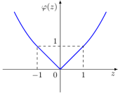
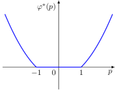
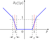
Figure 1: From left to right, the description of function $\varphi(z)$, its Fenchel conjugate $\varphi^{*}(p)$ and the regularization of $\varphi^{*}(p)$.

We recall that the Fenchel conjugate of an integral functional is an integral of the Fenchel conjugate of the corresponded integrand, i.e.

$$\left(\int_{D}f(p(x))dx\right)^{*}=\int_{D}f^{*}(p^{*}(x))dx.$$

For more details on this topic, we refer to [9]. We are going to apply this fact to calculate the conjugate of $m(s)$. For every $\lambda\in\mathbb{R}$,

$$m^{*}(\lambda) =\sup_{s\in\mathbb{R}}\left\{\lambda s-m(s)\right\}=-\inf_{u\in H^{1}_{0}(D)}\left\{\int_{D}\varphi(\nabla u)-\lambda\int_{D}u\right\}$$

$$=-\inf_{u\in H^{1}_{0}(D)}\sup_{p\in L^{2}(D;\mathbb{R}^{2})}\left\{\int_{D}p\cdot\nabla u-\int_{D}\varphi^{*}(p)-\lambda\int_{D}u\right\}$$

The second equality occurs with a replacement of the functional $\int_{D}\varphi(\nabla u)$ by a Fenchel conjugate. We regard that the functional

$$p\mapsto\inf_{u\in H^{1}_{0}(D)}\left\{\int_{D}p\cdot\nabla u-\int_{D}\varphi^{*}(p)-\lambda\int_{D}u\right\}$$

is finite if and only if $-\operatorname{div}p=\lambda$. So, by passing the inf-sup permutation argument, $m^{*}(\lambda)$ can be rewritten as

(40) $$m^{*}(\lambda)=\inf\left\{\int_{D}\varphi^{*}(p):p\in L^{2}(D;\mathbb{R}^{2}),-\operatorname{div}p=\lambda\right\}.$$

Furthermore, optimal solutions of $m(s)$ and $m^{*}(\lambda)$ are characterized by certain optimality conditions

$$\begin{cases}u\text{\; solution to \;}m(s)\\ p\text{\; solution to \;}m^{*}(\lambda)\\ \lambda\in\partial m(s)\end{cases}\qquad\Longleftrightarrow\qquad\begin{cases}\int_{D}u=s\\ -\operatorname{div}p=\lambda\\ p\in\partial\varphi(\nabla u)\text{\; a.e. \;}\end{cases}$$

Many interesting properties of functions $m(s)$ and $m^{*}(\lambda)$ were studied in [1]. One of them which is obviously seen is that the Fenchel equality is satisfied

$$m(s)+m^{*}(\lambda)=s\lambda,$$

since $\lambda\in\partial m(s)$.

We shall focus on the inf-sup formulation of $m^{*}(\lambda)$ which is adapted within our numerical schemes. But we must notice that $\varphi^{*}$ is neither strictly convex and nor differentiable on the unit circle $\{p\in\mathbb{R}^{2}:|p|=1\}$. A regularization for $\varphi^{*}$ should be done before enforcing the algorithms. See Figure 1 for visualization. Instead of taking the subgradient of $\varphi^{*}$, we regularize it by removing the discontinuities with an $\varepsilon$-affine symmetric connection

$$\partial\varphi^{*}_{\varepsilon}(p)=\begin{cases}\frac{2+\varepsilon}{2\varepsilon}\left(|p|+\frac{\varepsilon}{2}-1\right)\frac{p}{|p|}&\text{\; if \;}||p|-1|\leq\frac{\varepsilon}{2}\\ \partial\varphi^{*}(p)&\text{\; otherwise. \;}\end{cases}$$

It is ready to find a saddle point of the problem with $\varepsilon$-regularization.

The solution of such a problem in the context of shape optimization of thin torsion rods exhibits regions where $u$ is constant corresponding to regions without material, regions where $|\nabla u|\geq 1$ corresponds to the optimal region for the material in order to struggle torsion. Regions where $0<|\nabla u|<1$ describes the regions of homogenized material for which the convexity of the Lagrangian is not strict. This makes the problem nontrivial. Depending on the mass constraint, such a homogenization region can appear (low mass constraint leading to the so-called "homogeneous solution") or not ("special solution"). To answer the question whether an optimal design contains some homogenization region is equivalent to investigate when the special solution exists. And naturally, we wonder in which domain $D$ special solutions present. These are still open issue. In Figure 2, the magnitude of the gradient of the solution is plotted, a special solution can be found in the left figure, a homogenized solution is in the middle with weak gradient (lower than $1$) on regions limited by thick lines corresponding to $|\nabla u|=1$. In the right figure, the value $\lambda$ is close to the critical Cheeger constant while as we see, the optimal shape becomes thinner and tends to the boundary of the Cheeger set of the domain $D$ [12].

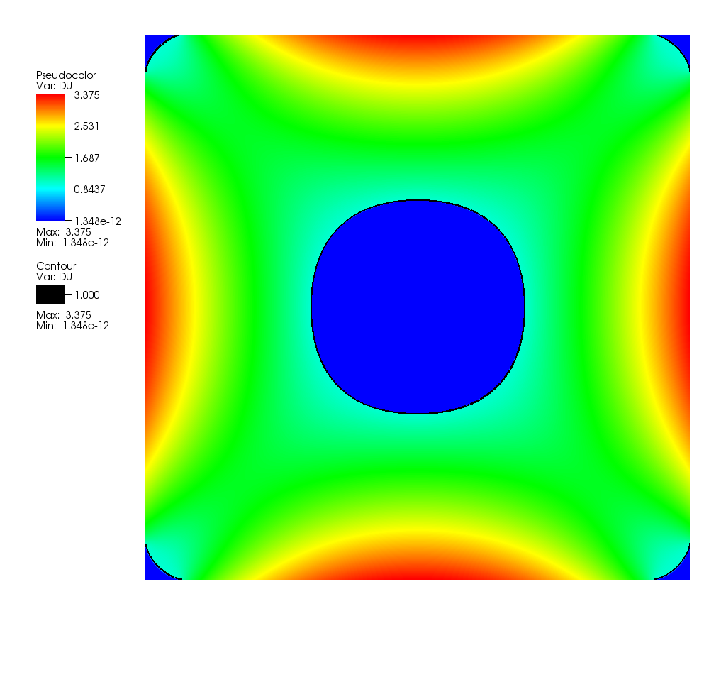
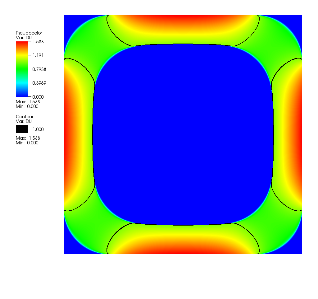
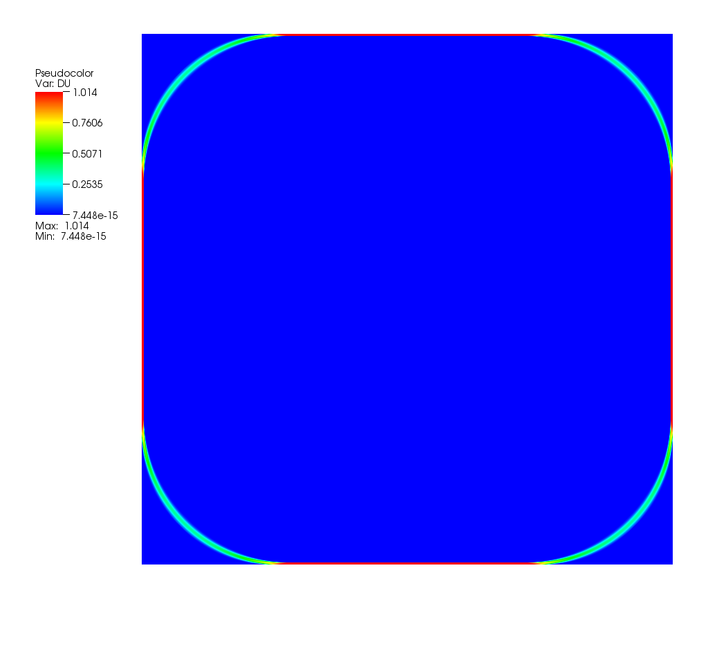
Figure 2: Special (left) and homogenized (middle and right) solutions depending on the mass constraint.

It is easy to see that if $D$ is a symmetric simple connected domain then solutions of $m(s)$ are symmetric. When $D$ is a square, the symmetrization allows dividing $D$ in four parts. Without lost of generality, let us describe the discretization settings with $D=[0,0.5]^{2}$ instead of unit square. Let $x=(x_{1},x_{2})$, $p=(p_{1},p_{2})$. The subdivision leads to the appearance of extra boundary conditions

$$u(\cdot,0.5)=u(0.5,\cdot)=0$$

$$p_{1}(0,\cdot)=p_{2}(\cdot,0)=0.$$

We shall implement our algorithms with space discretization on staggered MAC grids [10]. This choice leads to discretizations satisfying $\operatorname{div}^{h}=-(\nabla^{h})^{*}$, where the superscript denote the discretization with a mesh size $h$. $\nabla^{h}$ stands for discrete gradient operator.

We provide an explicit iterative process in discrete scheme with

(41) $$\begin{cases}p_{n+1}^{h}=p_{n}^{h}+\alpha(\nabla^{h}\overline{u}_{n}^{h}-\partial\varphi^{*}_{\varepsilon}(p_{n}^{h}))\\ u_{n+1}^{h}=\Pi_{C}^{h}(u_{n}^{h}+\beta(\operatorname{div}^{h}(p^{h}_{n+1})+\lambda))\\ \overline{u}^{h}_{n+1}=2u^{h}_{n+1}-u^{h}_{n}.\end{cases}$$

where $\Pi_{C}^{h}$ is the discretized projection. In this case, the projection is just simple to keep the boundary condition $u=0$ on $\partial D$. Since Lipschitz constants $L_{f}=0$, $L_{g}=(2+\varepsilon)/2\varepsilon$, the positive parameters $\alpha,\beta$ should be chosen such that

$$\alpha<\frac{4\varepsilon}{2+\varepsilon},\qquad\alpha\beta c_{h}^{2}+\frac{\alpha(2+\varepsilon)}{4\varepsilon}\leq 1\qquad\text{\; with \;}c_{h}:=||\nabla^{h}||=\frac{2\sqrt{2}}{h}.$$

We remark that $\alpha<4$ and tends to $0$ as $\varepsilon\to 0$. But with the second condition, the product $\alpha\beta$ should be of order $O(h^{2})$.

In the point of view of implicit scheme, the proposed convergent process reads

(42) $$\begin{cases}p_{n+1}^{h}=p_{n}^{h}+\alpha(\nabla^{h}\overline{u}_{n}^{h}-\partial\varphi^{*}_{\varepsilon}(p_{n}^{h}))\\ u_{n+1}^{h}=u_{n}^{h}+\beta(I-\Delta^{h})^{-1}(\operatorname{div}^{h}(p^{h}_{n+1})+\lambda)\\ \overline{u}^{h}_{n+1}=2u^{h}_{n+1}-u^{h}_{n}.\end{cases}$$

We replaced $\operatorname{div}^{h}(p^{h}_{n+1})+\lambda$ in the explicit process by $\widetilde{u}_{n}=(I-\Delta^{h})^{-1}(\operatorname{div}^{h}(p^{h}_{n+1})+\lambda)$ which is solution of the equations

$$\begin{cases}(I-\Delta^{h})v=\operatorname{div}^{h}(p^{h}_{n+1})+\lambda\\ v=0\quad\text{\; on \;}\quad\partial D\end{cases}$$

The projection $\Pi_{C}^{h}$ then disappears since the boundary condition on $u$ is added within resolving $\widetilde{u}_{n}$. Moreover, the positive parameters are simplified

$$\alpha<\frac{4\varepsilon}{2+\varepsilon},\qquad\alpha\beta+\frac{\alpha(2+\varepsilon)}{4\varepsilon}<1.$$

We see that the choices of $\alpha,\beta$ now do not depend on $c_{h}$ and thus, the product $\alpha\beta$ is of order $O(1)$ with respect to $h$. Nevertheless, the step size $\alpha$ is still restricted by small $\varepsilon$.

The regularizing parameter $\varepsilon$ is linked to the grid size, in practice we take for instance $\varepsilon=3h$. This relation makes the step size $\alpha$ be of order of $h$ for the implicit algorithm (42). It leads to introduce a new algorithm with $\kappa$ sub-iterations on the explicit part of (42), in implementation $\kappa=50$:

(43) $$\begin{cases}p_{n+1,0}^{h}=p_{n,\kappa}^{h}\\ p_{n+1,k+1}^{h}=p_{n+1,k}^{h}+\frac{\alpha}{\kappa}(\nabla^{h}\overline{u}_{n}^{h}-\partial\varphi^{*}_{\varepsilon}(p_{n+1,k}^{h})),\qquad k=0,1,...,\kappa-1\\ u_{n+1}^{h}=u_{n}^{h}+\beta(I-\Delta^{h})^{-1}(\operatorname{div}^{h}(p_{n+1,\kappa}^{h})+\lambda)\\ \overline{u}^{h}_{n+1}=2u^{h}_{n+1}-u^{h}_{n}.\end{cases}$$

The algorithm (43) allows $\alpha$ to be $\kappa$ times bigger and then reduces the number of iterations in $n$.

From now on, the algorithm (43) is called Implicit Sub-iteration Scheme (ISS), the algorithm (42) is called Implicit Scheme (IS) and the algorithm (41) is called Explicit Scheme (ES).

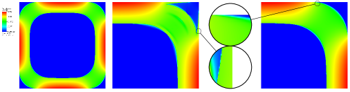
Figure 3: Case $\lambda=5$ for (ES) on the left, (IS) in the middle, (ISS) on the right, for the same grid size.

In Figure 3, we present the Euclidean norm of the gradient of a solution, i.e. $|\nabla u|$. The left figure shows an expected solution with the explicit scheme. The centered and the right ones are in a quarter domain which are done with implicit methods (IS) and (ISS), respectively. We see that in implicit scheme (IS), the contact zones are still not tangent to the boundary of domain (the region on which it is difficult to converge the algorithm). And, the (IS) algorithm, expected to be slower than (ISS), introduces an other drawback with numerical artefacts.

In the processes (42)-(43), the inverse Laplacian computation is the most costly. The computational cost thus depends highly on the solver used for the inverse Laplacian operator. If one uses a multigrid or a FFT solver, it can be of order $\displaystyle\frac{1}{h^{2}\log h}$. Besides, handling a multigrid solver, for instance AGMGPAR (A parallel version of Algebraic Multigrid method), see [13], and MAC scheme, it easy to implement our algorithms with MPI (Massage Passing Interface) library which provides an effective environment for parallel computation. In the following computations, comparisons between the different schemes are done with a fixed number of process to $6$, leading to good scalability for all methods.

Before comparing the computational cost, we ensure that the algorithms converge to the exact solution as the grid size $h$ goes to zero. We then consider a case in which the unique exact solution is known, that is when $D$ is a disk. In such a case, the solution is a special solution and it is radial with mass concentrated on the periphery and with an internal radius of $\overline{R}=\frac{2}{\lambda}$ (see Figure 4), see [1] for the expression of the exact solution.

Figure 4: Exact solution when the constraint domain $D$ is a disk.

We are then able to compute the numerical internal radius $r_{N}$, $R_{N}$ defined respectively as the maximal value of radius where $|\nabla u|$ is smaller than a half and the minimal value of radius where $|\nabla u|$ is bigger than one. The error on the internal radius is measured as a number of cells for different cell sizes. The radius error is of order of a half of grid size whatever the grid, as shown on Figure 5.

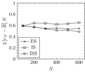
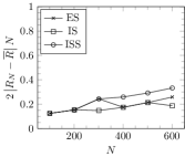
Figure 5: Graph of $2{|r_{N}-\overline{R}|}{N}$ and $2{|R_{N}-\overline{R}|}{N}$ with respect to the grid size $N$.

We are now concerned with the comparison of computational cost between schemes (ES), (IS), (ISS) in the case where $\lambda=5$, for a unitary square $D$, so that an homogeneous solution occurs.

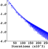
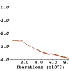
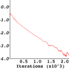
Figure 6: Convergence of algorithms with criterion $\|\operatorname{div}p+\lambda\|_{L^{2}}<10^{-4}$ in case $\lambda=5$. From left to right, the first figure is in (ES), the second with (IS), and the last one is done with (ISS)

We remark that we have to well pay for the cost of inverse Laplacian operator. So, the choice of solvers should be carefully considered. But, the positive side of semi-implicit scheme is to reduce globally many iterations of the iterative process. When the projections on convex sets become more expensive, this reduction of iteration will evidently save the computational time. At the moment, semi-implicit scheme is the most efficient, see Table 1, Figure 6 and Figure 7.

$\|\operatorname{div}p+\lambda\|_{L^{2}}<10^{-4}$ with MPI in 6 processes
$N$	iterations			time (seconds)
	ES	IS	ISS	ES	IS	ISS
101	9451	763	360	0.59	12.75	5.84
201	21647	1340	545	4.92	47.63	20.18
301	34719	1857	733	17.96	92.01	39.93
501	59438	2822	856	113.29	311.92	121.36
801	98484	4072	1251	848.15	819.10	467.12
1201	154107	5777	1596	3590.69	2625.47	1460.76
1701	232793	7629	2038	11520.75	7642.35	3876.28
1921	268999	8507	2230	17183.18	11174.52	5717.89

Table 1: Comparison of three methods in iterations and computational time in case $\lambda=5$. The stop criterion is $\|\operatorname{div}p+\lambda\|_{L^{2}}<10^{-4}$. They are implemented with MPI in 6 processes.

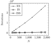
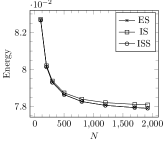
Figure 7: Comparison of three methods in term of iterations, computational time, convergence of energy function in case $\lambda=5$.

5 Conclusion

The generalized explicit scheme for searching saddle points of Lagrangians of type (3) is convergent and widely applicable. The main contribution of this article is to propose a semi-implicit extension of such an algorithm. It remains convergent under less restrictive constraint on numerical parameters. Non differentiability can possibly occur in Lagrangians, and in this case, to fix it, we regularize derivatives of Lagrangians, with a smoothing parameter linked to the space discretization parameter. The semi-implicit scheme, coupled to a splitting method for the rapidly computed explicit part, provides a robust acceleration of the computational cost in comparison with the fully explicit one. The number of iterations in order to reach a precise convergence is widely reduced as shown in Section 4. Even if an iteration is more costly for the semi-implicit algorithm, the global computational cost is clearly reduced, specially for fine grids and provides accurate solutions. Furthermore, such an algorithm can reveal even more performing than explicit scheme when Lipschitz constants functions $F$ and $G$ are lower and also if the Lagrangian contains large quadratic terms with respect to the $p$ variable. This algorithm has then been willingly tested on a stiff problem. In any case, the solver of a Laplacian type problem must be carefully chosen since it mainly contributes to the computational cost. Once set up, the heavier projections are, the more efficiency the semi-implicit scheme shows.

References

- [1] J. J. Alibert, G. Bouchitté, I. Fragalà, and I. Lucardesi, A nonstandard free boundary problem arising in the shape optimization of thin torsion rods, Interfaces Free Bound, 15 (2013), pp. 95–119.
- [2] H. Alt and L. Caffarelli, Existence and regularity for a minimum problem with free boundary, J. Reine Angew. Math., 325 (1981), pp. 105–144.
- [3] G. Bouchitté and I. Fragalà, Duality for non-convex variational problems, C. R. Math. Acad. Sci. Paris, 353 (2015), pp. 375–379.
- [4] G. Bouchitté and I. Fragalà, A duality theory for non-convex variational problems, submitted, (2017), https://arxiv.org/pdf/1607.02878.pdf.
- [5] G. Bouchitté and M. Phan, A duality recipe for non convex variational problems, submitted.
- [6] G. Bouchitté and P. Seppecher, Cahn and hilliard fluid on an oscillating boundary, Motion by mean curvature and related topics (Trento, 1992), (1994), pp. 23–42.
- [7] A. Chambolle and T. Pock, A first-order primal-dual algorithm for convex problems with applications to imaging, Journal of mathematical imaging and vision, 40 (2011), pp. 120–145.
- [8] A. Chambolle and T. Pock, On the ergodic convergence rates of a first-order primal–dual algorithm, Mathematical Programming, 159 (2016), pp. 253–287.
- [9] I. Ekeland and R. Temam, Analyse convexe et problemes variationneles, Dunod Gauthier-Villars, Paris, (1974).
- [10] F. H. Harlow and J. E. Welch, Numerical calculation of time-dependent viscous incompressible flow of fluid with free surface, The physics of fluids, 8 (1965), pp. 2182–2189.
- [11] M. Kallio and A. Ruszczynski, Perturbation methods for saddle point computation, (1994).
- [12] B. Kawohl and T. Lachand-Robert, Characterization of cheeger sets for convex subsets of the plane, Pacific journal of mathematics, 225 (2006), pp. 103–118.
- [13] Y. Notay, User’s guide to agmg, Electronic Transactions on Numerical Analysis, 37 (2010), pp. 123–146.
- [14] T. Pock, D. Cremers, H. Bischof, and A. Chambolle, An algorithm for minimizing the mumford-shah functional, in Computer Vision, 2009 IEEE 12th International Conference on, IEEE, 2009, pp. 1133–1140.
- [15] L. D. Popov, A modification of the arrow-hurwicz method for search of saddle points, Mathematical notes of the Academy of Sciences of the USSR, 28 (1980), pp. 845–848.
- [16] W. Rudin, Functional analysis. international series in pure and applied mathematics, 1991.