Fluid dynamics of out of equilibrium boost invariant plasmas

Jean-Paul Blaizot Institut de Physique Théorique, Université Paris Saclay, CEA, CNRS, F-91191 Gif-sur-Yvette, France Li Yan Department of Physics, McGill University, 3600 rue University Montréal, QC Canada H3A 2T8

Abstract

By solving a simple kinetic equation, in the relaxation time approximation, and for a particular set of moments of the distribution function, we establish a set of equations which, on the one hand, capture exactly the dynamics of the kinetic equation, and, on the other hand, coincide with the hierarchy of equations of viscous hydrodynamics, to arbitrary order in the viscous corrections. This correspondence sheds light on the underlying mechanism responsible for the apparent success of hydrodynamics in regimes that are far from local equilibrium.

Introduction.

The observation that the evolution of the quark-gluon plasma produced in ultra-relativistic heavy ion collisions is well described by viscous hydrodynamic equations raises a number of interesting questions that are very much debated presently Florkowski:2017olj . Traditional understanding of hydrodynamics would imply that the system has reached local equilibrium, and the small viscosity extracted from the analysis of the data is suggestive of short mean free paths. However, works on strongly coupled plasmas, using in particular holography techniques, indicate that viscous hydrodynamics works even when large anisotropies, that signal departure from local equilibrium, are still present Heller:2011ju . At the same time, there is evidence that hydrodynamics is capable of describing small colliding systems, for which no clear separation a priori exists between microscopic and macroscopic scales (see e.g. the recent discussion in Romatschke:2017vte ; Florkowski:2017olj and references therein).

Recently, it has been argued that part of the success of hydrodynamics could be due to the existence of a stable attractor, to which the solution of the dynamical equations quickly converge before eventually reaching the viscous hydrodynamic regime Heller:2015dha . This suggestion has triggered many studies, some of which involve sophisticated mathematical developments Spalinski:2017mel ; Strickland:2017kux ; Romatschke:2017acs ; Denicol:2017lxn ; Behtash:2017wqg . In this paper, we would like to offer an alternative perspective on the issue, based on the simple, and physically motivated observation, that the main features of the dynamics of expanding plasmas are determined by the competition between the expansion itself, which is dictated by the external conditions of the collisions, and the collisions among the plasma constituents which generically tend to isotropize the particle momentum distribution functions. These two competing effects give rise to two independent fixed points of a suitably defined dynamical quantity. Many recent results find a natural interpretation in the interplay between these two fixed points.

As in many works on this issue, we focus on the paradigmatic example of the Bjorken flow Bjorken:1982qr , and consider an expanding system of massless particles characterized by a distribution function $f$ whose time evolution is given by a kinetic equation. Symmetry allows us to reconstruct the full space-time history of the system from the knowledge of what happens in a slice centered around the plane $z=0$ where the collision takes place. The distribution function in that slice depends solely on the momentum of the particle and the (proper) time $\tau$ , i.e., $f=f({\bf p},\tau)$ . Using a relaxation time approximation for the collision kernel, we can then write the following simple kinetic equation Baym:1984np

\left[\partial_{\tau}-\frac{p_{z}}{\tau}\partial_{p_{z}}\right]f({\bf p},\tau)=-\frac{f({\bf p},\tau)-f_{\rm eq}(p/T)}{\tau_{R}}.

(1)

Here $f_{\rm eq}(p/T)$ is a function that depends only on $p=|{\bf p}|$ and an effective temperature $T(\tau)$ which is determined by requiring that the energy density calculated with $f_{\rm eq}(p/T)$ and $f({\bf p},\tau)$ takes the same value, $\varepsilon\propto T^{4}$ , at all times. The kinetic equation (1) makes transparent the competition alluded to above, between the expansion and the collisions. In the absence of the collision term, the expansion, controlled by the term $-p_{z}/\tau$ in the left hand side, leads to a flattened distribution, $f({\bf p},\tau)\to f_{0}(p_{z}\tau,{\bf p}_{\perp})$ , where $f_{0}$ is the initial distribution and ${\bf p}_{\perp}$ is the component of the momentum orthogonal to the $z$ -axis. On the other hand, the collision term in the right hand side drives the distribution towards isotropy, at a rate controlled by the relaxation time $\tau_{R}$ .

Kinetics in terms of ${\cal L}$ -moments.

Although Eq. (1) can be easily solved numerically, more insight can be gained by using an alternative, albeit approximate, approach that eliminates from the description as much of irrelevant information as possible. Thus, in this paper, instead of considering the full distribution $f({\bf p},\tau)$ , we focus on some of its moments, introduced in Ref. Blaizot:2017lht :

{\cal L}_{n}=\int\!\!\!\frac{d^{3}{\bf p}}{(2\pi)^{3}p^{0}}|{\bf p}|^{2}P_{2n}(p_{z}/|{\bf p}|)f({\bf p},\tau),

(2)

where $P_{2n}$ is a Legendre polynomial of order $2n$ . The moments ${\cal L}_{n}$ with $n\geq 1$ describe the momentum anisotropy of the system. In particular ${\cal L}_{1}={\mathcal{P}}_{L}-{\mathcal{P}}_{T}$ reflects the asymmetry between longitudinal ( $P_{L})$ and transverse ( $P_{T}$ ) pressures. The moment ${\cal L}_{0}$ coincides with the energy density, ${\cal L}_{0}=\varepsilon=P_{L}+2P_{T}$ . Observe that the momentum weight of the integration in Eq. (2) is always $|{\bf p}|^{2}$ , instead of being an increasing power of $|{\bf p}|$ as is the case in more standard approaches (see e.g. Bazow:2016oky ). Thus, the ${\cal L}_{n}$ ’s contain little information on the radial shape of the momentum distribution, preventing us for instance to reconstruct from them the full distribution. However, this radial shape plays a marginal role in the isotropization of the momentum distribution, which is our main concern here. Note that all the ${\cal L}_{n}$ have the same dimension.

By using the recursion relations among the Legendre polynomials, we can recast Eq. (1) into the following (infinite) set of coupled equations

		$\displaystyle\frac{\partial{\cal L}_{n}}{\partial\tau}=$	$\displaystyle-\frac{1}{\tau}\left[a_{n}{\cal L}_{n}+b_{n}{\cal L}_{n-1}+c_{n}{\cal L}_{n+1}\right]-\frac{{\cal L}_{n}}{\tau_{R}}\quad(n\geq 1)$
		$\displaystyle\frac{\partial{\cal L}_{0}}{\partial\tau}=$	$\displaystyle-\frac{1}{\tau}\left[a_{0}{\cal L}_{0}+c_{0}{\cal L}_{1}\right],$		(3)

where the coefficients $a_{n},b_{n},c_{n}$ are pure numbers


$\displaystyle a_{n}=$	$\displaystyle\frac{2(14n^{2}+7n-2)}{(4n-1)(4n+3)}\,,\quad b_{n}=\frac{(2n-1)2n(2n+2)}{(4n-1)(4n+1)}\,,$
$\displaystyle c_{n}=$	$\displaystyle\frac{(1-2n)(2n+1)(2n+2)}{(4n+1)(4n+3)},$	(4a)

entirely determined by the free streaming part of the kinetic equation. Note that the collision term does not affect directly the energy density, but only the moments with $n\geq 1$ . In fact, if one ignores the expansion, i.e., set $a_{n}=b_{n}=c_{n}=0$ , the moments evolve according to

\displaystyle{\cal L}_{0}(\tau)={\cal L}_{0}(0),\quad{\cal L}_{n}(\tau)={\cal L}_{n}(0)\,{\rm e}^{-\tau/\tau_{R}}.

(5)

This solution illustrates the role of the collisions in erasing the anisotropy of the momentum distribution as the system approaches equilibrium. Of course, the expansion prevents the system to ever reach this trivial equilibrium fixed point: instead, the system goes into an hydrodynamical regime, as we shall discuss later.

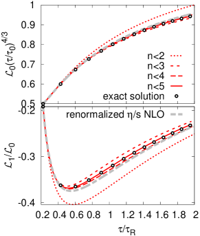
The system of Eqs. (Kinetics in terms of ${\cal L}$ -moments.) lends itself to simple truncations. Thus by ignoring all moments of order higher than $n$ , one obtains a finite set of $n+1$ equations that can be easily solved. The accuracy of such a procedure can be judged from Fig. 1, where the moments obtained from various truncations are compared with those of the numerical solution of Eq. (1) for an initial distribution typical of a heavy ion collision: $f(\tau_{0},p_{T},p_{z})=f_{0}\Theta\left(Q_{s}-\sqrt{\xi^{2}p_{z}^{2}+p_{T}^{2}}\right)$ with $f_{0}=0.1$ , $\xi=1.5$ , corresponding to an initial momentum anisotropy ${\mathcal{P}}_{L}/{\mathcal{P}}_{T}\approx 0.5$ , and $\tau_{0}=Q_{s}^{-1}$ Blaizot:2017lht . Already the lowest order truncation at $n=1$ captures the qualitative behaviour of the full solution. Note that the approach to the exact solution is alternating, which offers an estimate of the truncation error. The energy density approaches smoothly the hydrodynamic regime as $\tau\gtrsim\tau_{R}$ , while the non monotonous behaviour of the ratio ${\cal L}_{1}/{\cal L}_{0}$ reflects the competition between expansion and collisional effects that we now analyze in more detail, starting with the free streaming regime.

Refer to caption — Figure 1: (Color online) Comparison of the ${\cal L}$ -moment equations obtained from various truncation of Eqs. (Kinetics in terms of ${\cal L}$ -moments.) (lines), with those of the numerical solution of the kinetic equation (1) (symbols).

The free streaming fixed point.

The free streaming regime is described by Eq. (Kinetics in terms of ${\cal L}$ -moments.) where one ignores the collision term. It is not hard to see that the resulting equation possesses a stable solution at large time, in which all moments decay as $1/\tau$ and are proportional to each other: ${\cal L}_{n}(\tau)=A_{n}{\cal L}_{0}(\tau)$ , where the dimensionless constants $A_{n}$ characterize the moments of a distribution that is flat in the $p_{z}$ direction Blaizot:2017lht

\displaystyle A_{n}=P_{2n}(0)=(-1)^{n}\,\frac{(2n-1)!!}{(2n)!!}.

(6)

Note that $A_{1}=-1/2$ , corresponding to a vanishing longitudinal pressure. As for the factor $1/\tau$ it reflects the conservation of the energy in the increasing comoving volume ( $\tau\varepsilon(\tau)={\rm cste}$ ). Defining

g_{n}(\tau)=\tau\partial_{\tau}\ln{\cal L}_{n},

(7)

we get from Eq. (Kinetics in terms of ${\cal L}$ -moments.)

g_{n}(\tau)=-a_{n}-b_{n}\frac{{\cal L}_{n-1}}{{\cal L}_{n}}-c_{n}\frac{{\cal L}_{n+1}}{{\cal L}_{n}}-(1-\delta_{n0})\frac{\tau}{\tau_{R}}.

(8)

The solution above corresponds to a fixed point for the $g_{n}$ ’s. Dropping the last term, and using the expression (6) for the ratio of moments, one indeed verifies easily that for all $n$ , $g_{n}(\tau)=-1$ . If the initial ratios of moments are chosen according to Eq. (6), the $g_{n}$ ’s remain constant in time (all equal to $-1$ ), whereas for arbitrary initial conditions, they will reach the fixed point at late time. Note that the fixed point obtained from a truncation at a finite order differs slightly from $-1$ : for instance, in the simplest truncation at $n<2$ , $g_{0}=g_{1}=-0.92937$ instead of -1, and $A_{1}\approx-0.6$ instead of $-0.5$ .

The hydrodynamic fixed point.

We know from our previous study Blaizot:2017lht that, at late times, ${\cal L}_{n}(\tau)$ admits the following expansion, analogous to a gradient expansion¹¹1For Bjorken flow, the gradient expansion coincides with an expansion in powers of $\tau_{R}/\tau$ , which may also be viewed as an expansion in Knudsen number.

{\cal L}_{n}(\tau)=\frac{1}{\tau^{n}}\sum_{m=0}^{\infty}\frac{\alpha_{n}^{(m)}}{\tau^{m}}\,.

(9)

The coefficients in Eq. (9) are nothing but transport coefficients, except for the first moment, equal to the energy density, i.e., $\alpha_{0}^{(m)}=\varepsilon\delta_{m0}$ . The behavior of $\varepsilon(\tau)$ at large time is obtained from Eq. (Kinetics in terms of ${\cal L}$ -moments.), ignoring the contribution of ${\cal L}_{1}$ . Since $a_{0}=4/3$ , this behavior is that of ideal hydrodynamics, $\varepsilon(\tau)\sim\tau^{-4/3}$ , and hence $T(\tau)\sim\tau^{-1/3}$ . The leading and sub-leading transport coefficients in Eq. (9) can be determined analytically. To do so, we return to Eq. (8) and note that a cancellation of the relaxation term has to occur in order to eliminate the exponential decaying contributions to the moments. This cancellation determines the leading order coefficient, viz. $\alpha_{n}^{(0)}=(-\tau_{R})^{n}\varepsilon\prod_{i=1}^{n}b_{i}$ . In particular, $\alpha_{1}^{(0)}=-b_{1}\tau_{R}\varepsilon=-2\eta$ , with $\eta$ the shear viscosity. In a conformal invariant setting Baier:2007ix , we allow $\tau_{R}$ to depend on the temperature, with $\tau_{R}T(\tau)$ kept constant²²2The constant is given by $\tau_{R}T(\tau)=5\eta/s$ , with the entropy density given by $s=4\varepsilon/(3T)$ .. Then, one gets $\alpha_{n}^{(0)}\sim\tau^{-(4-n)/3}$ which implies that in leading order, ${\cal L}_{n}(\tau)\sim\tau^{-(4+2n)/3}$ . This defines the hydrodynamic fixed point, $g_{n}(\tau)=-(4+2n)/3$ .³³3In the conformal invariant setting, this result could also be obtained from a simple dimensional analysis. For a time-independent relaxation time, the hydrodynamic fixed point is instead $g_{n}(\tau)=-(4+3n)/3$ . The sub-leading coefficients in Eq. (9) are then fixed by imposing this asymptotic power law, which yields

\frac{\alpha_{n}^{(1)}}{\alpha_{n}^{(0)}}=\tau_{R}b_{n}\left[\frac{1}{b_{n}}\left(\frac{4+2n}{3}-a_{n}\right)-\frac{\alpha_{n-1}^{(1)}}{\alpha_{n}^{(0)}}\right]\,.

(10)

The first few coefficients reproduce the values of known transport coefficients Blaizot:2017lht ; Teaney:2013gca , for instance $\alpha_{2}^{(0)}=\frac{64}{105}\,\varepsilon\tau_{R}^{2}=\frac{4}{3}(\lambda_{1}+\eta\tau_{\pi})$ , $\alpha_{1}^{(1)}=-\frac{32}{315}\,\varepsilon\tau_{R}^{2}=\frac{4}{3}(\lambda_{1}-\eta\tau_{\pi})$ , with $\lambda_{1}$ and $\tau_{\pi}$ as defined in Baier:2007ix .

The attractor.

One may define an attractor solution as the particular solution of Eqs. (Kinetics in terms of ${\cal L}$ -moments.) which, at short time, coincides with the free streaming fixed point $g_{n}=-1$ , and at large time goes over to the hydrodynamic fixed point. It can be determined numerically, by solving Eqs. (Kinetics in terms of ${\cal L}$ -moments.) with initial conditions specified by the constants (6). We have checked that $g_{0}$ obtained in this way is consistent with what was found by other methods in Ref. Romatschke:2017vte ; Heller:2015dha . The solution, obtained by truncating Eqs. (Kinetics in terms of ${\cal L}$ -moments.) at $n<20$ , is displayed in Fig. 2 for the first few $g_{n}(\tau)$ . The universal character of the curves is worth emphasizing.

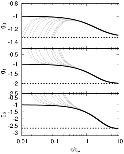
All the $g_{n}$ ’s behave in the same way, interpolating between the two fixed point $g_{n}\approx-1$ ⁴⁴4Because of the truncation at $n<20$ , the fixed point does not lie exactly at $-1$ , but at $-1.00294$ and $g_{n}=-(4+2n)/3$ , the transition occurring when $\tau\sim\tau_{R}$ .

Hydrodynamics.

At this point, we note that the truncations of the equations (Kinetics in terms of ${\cal L}$ -moments.) for the moments are closely related to successive viscous corrections to hydrodynamics. We have already seen that the lowest order truncation, i.e., with only ${\cal L}_{0}$ non vanishing, is identical to ideal hydrodynamics. The truncation at order $n=1$ yields two coupled equations that can be cast in the form

\displaystyle\partial_{\tau}\epsilon=-\frac{4}{3}\frac{\epsilon}{\tau}+\frac{\Pi}{\tau}\,,\quad\partial_{\tau}\Pi=\frac{4}{3}\frac{\eta}{\tau\tau_{R}}-a_{1}\frac{\Pi}{\tau}-\frac{\Pi}{\tau_{R}}\,,

(11)

where $\Pi\equiv-c_{0}{\cal L}_{1}$ , and we used the leading order relation ${4}{\eta}/(3{\tau\tau_{R})}=c_{0}b_{1}{\varepsilon}/{\tau}.$ These are just the second order viscous hydrodynamic equations, in the version of Ref. Denicol:2012cn with $\beta_{\pi\pi}=a_{1}=38/21$ . The first order viscous hydrodynamics uses the solution of the second equation (11) for small $\tau_{R}$ , viz. $\Pi\simeq 4\eta/(3\tau)=(16/45)\varepsilon(\tau_{R}/\tau)$ . The much studied (lack of) convergence of the hydrodynamic gradient expansion in the context of Bjorken flow concerns the series of the coefficients $\alpha_{1}^{(n)}$ in Eq. (9) for ${\cal L}_{1}\sim\Pi$ , as can be deduced from the solution of the coupled equations (11) at large time Spalinski:2017mel .

Taking higher moments into account is tantamount to including higher order viscous corrections. For instance, the lowest order contribution of ${\cal L}_{2}$ to the equation for ${\cal L}_{1}$ reads

\frac{c_{0}c_{1}{\cal L}_{2}}{\tau}=\frac{c_{1}b_{2}}{c_{0}b_{1}\varepsilon}\frac{\Pi^{2}}{\tau}

(12)

where we have used Eqs. (9) and (10) to write ${\cal L}_{2}=\alpha_{2}{(0)}/\tau^{2}=\alpha_{2}^{(0)}/(\alpha_{1}^{(0)}c_{0})^{2}\Pi^{2}$ . It can be verified that the correction (12) coincides with the third order viscous correction derived in Ref. Jaiswal:2013vta . Obviously, it would be straightforward to obtain in this way higher order viscous corrections, if needed. Note that since $b_{n}\sim n$ at large $n$ , $\alpha_{n}^{(0)}\propto n!$ , and the series of the $\alpha_{n}^{(0)}$ suffers from the same lack of convergence as that of the $\alpha_{1}^{(n)}$ determining the viscous part of the energy momentum tensor.

Renormalization of $\eta/s$ .

Alternatively, the effects of the higher moments can be treated as a renormalization of the viscosity entering the equations for ${\cal L}_{0}$ and ${\cal L}_{1}$ . To see that, rewrite the equation for ${\cal L}_{1}$ as

\displaystyle\partial_{\tau}{\cal L}_{1}=-\frac{1}{\tau}\left(a_{1}{\cal L}_{1}+b_{1}{\cal L}_{0}\right)-\left[1+\frac{c_{1}\tau_{R}}{\tau}\frac{{\cal L}_{2}}{{\cal L}_{1}}\right]\frac{{\cal L}_{1}}{\tau_{R}},

(13)

with $Z_{\eta/s}^{-1}\equiv\left[1+\frac{c_{1}\tau_{R}}{\tau}\frac{{\cal L}_{2}}{{\cal L}_{1}}\right]$ . The dimensionless ratio ${\cal L}_{2}/{\cal L}_{1}$ is analytically related to the attractor $g_{2}(\tau)$ , the leading order result being

\frac{{\cal L}_{2}}{{\cal L}_{1}}=-\frac{b_{2}}{a_{2}+{\tau}/{\tau_{R}}+g_{2}(\tau)}\,.

(14)

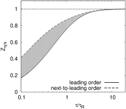
Sub-leading contributions involving higher $g_{n}$ ’s can be obtained iteratively. The quantity $Z_{\eta/s}$ in Eq. (13) then defines a multiplicative renormalizaiton of $\eta/s$ (or equivalently of $\tau_{R}$ : $\tau_{R}\to Z_{\eta/s}\tau_{R}$ ), whose variation with $\tau_{R}$ is displayed in Fig. 3. Since successive corrections alternate in sign, the grey band provides an estimate of the error. At large times, corresponding to a system in local thermal equilibrium, $Z_{\eta/s}$ is close to unity. For systems far-from-equilibrium, $Z_{\eta/s}$ tends to vanish. Thus, in systems out-of-equilibrium, higher order viscous corrections effectively reduce the value of $\eta/s$ entering the second order viscous hydrodynamic equations, an effect first pointed out by Lublinsky and Shuryak Lublinsky:2007mm . As can be seen on Fig. 1 (grey dashed line), this simple renormalization brings the solution of the lowest non trivial truncation quite close to the exact solution. That is, with this correction, second order viscous hydrodynamics reproduces accurately the exact solution of the kinetic theory.

In summary, we have seen that it is possible for viscous hydrodynamics to describe accurately the evolution of boost invariant plasmas, even in regimes where the usual conditions of applicability of hydrodynamics are not satisfied. This is because the viscous hydrodynamic equations can be mapped into equations for moments of the momentum distribution that account exactly for the underlying kinetic theory. Although the present discussion relies on specific properties of Bjorken flow and the use of a simplified kinetic equation, we expect some general features to be robust, such as the existence of the free streaming and the hydrodynamic fixed points⁵⁵5In approaches based on holography, the hydrodynamic fixed point naturally emerges. However what plays the role of the free streaming fixed point in this context is unclear to us., joined by an attractor solution, or the renormalization of the effective viscosity. Clearly these results may have impact on the interpretation of heavy ion data and deserve further study.

Acknowledgements

LY is supported in part by the Natural Sciences and Engineering Research Council of Canada. We thank Jean-Yves Ollitrault for insightful comments on the manuscript.

References

(1) W. Florkowski, M. P. Heller and M. Spalinski, arXiv:1707.02282 [hep-ph].
(2) M. P. Heller, R. A. Janik and P. Witaszczyk, Phys. Rev. Lett. 108 (2012) 201602 [arXiv:1103.3452 [hep-th]].
(3) P. Romatschke, arXiv:1704.08699 [hep-th].
(4) M. P. Heller and M. Spalinski, Phys. Rev. Lett. 115 (2015) no.7, 072501 [arXiv:1503.07514 [hep-th]].
(5) M. Spalinski, arXiv:1708.01921 [hep-th].
(6) M. Strickland, J. Noronha and G. Denicol, arXiv:1709.06644 [nucl-th].
(7) P. Romatschke, arXiv:1710.03234 [hep-th].
(8) G. S. Denicol and J. Noronha, arXiv:1711.01657 [nucl-th].
(9) A. Behtash, C. N. Cruz-Camacho and M. Martinez, arXiv:1711.01745 [hep-th].
(10) J. D. Bjorken, Phys. Rev. D 27 (1983) 140.
(11) G. Baym, Phys. Lett. 138B (1984) 18.
(12) J. P. Blaizot and L. Yan, JHEP 1711, 161 (2017) doi:10.1007/JHEP11(2017)161 [arXiv:1703.10694 [nucl-th]].
(13) D. Bazow, G. S. Denicol, U. Heinz, M. Martinez and J. Noronha, Phys. Rev. D 94 (2016) no.12, 125006 [arXiv:1607.05245 [hep-ph]].
(14) R. Baier, P. Romatschke, D. T. Son, A. O. Starinets and M. A. Stephanov, JHEP 0804 (2008) 100 [arXiv:0712.2451 [hep-th]].
(15) D. Teaney and L. Yan, Phys. Rev. C 89 (2014) no.1, 014901 [arXiv:1304.3753 [nucl-th]].
(16) G. S. Denicol, H. Niemi, E. Molnar and D. H. Rischke, Phys. Rev. D 85 (2012) 114047 Erratum: [Phys. Rev. D 91 (2015) no.3, 039902] [arXiv:1202.4551 [nucl-th]].
(17) A. Jaiswal, Phys. Rev. C 88, 021903 (2013) [arXiv:1305.3480 [nucl-th]].
(18) M. Lublinsky and E. Shuryak, Phys. Rev. C 76 (2007) 021901 [arXiv:0704.1647 [hep-ph]].