Long-Range Correlation Underlying Childhood Language
and Generative Models

Abstract

Long-range correlation, a property of time series exhibiting long-term memory, is mainly studied in the statistical physics domain and has been reported to exist in natural language. Using a state-of-the-art method for such analysis, long-range correlation is first shown to occur in long CHILDES data sets. To understand why, Bayesian generative models of language, originally proposed in the cognitive scientific domain, are investigated. Among representative models, the Simon model was found to exhibit surprisingly good long-range correlation, but not the Pitman-Yor model. Since the Simon model is known not to correctly reflect the vocabulary growth of natural language, a simple new model is devised as a conjunct of the Simon and Pitman-Yor models, such that long-range correlation holds with a correct vocabulary growth rate. The investigation overall suggests that uniform sampling is one cause of long-range correlation and could thus have a relation with actual linguistic processes.

Keywords: Bayesian generative models of language, long-range correlation, autocorrelation function, vocabulary growth

1 Introduction

State-of-the-art Bayesian mathematical models of language include the Simon and Pitman-Yor models and their extensions (Pitman 2006) (Goldwater et al. 2011) (Lee and Wagenmakers 2014) (Chater and Oaksford 2008). These models have been not only successful in modeling language from a cognitive perspective but also applicable in natural language engineering (Teh 2006). They have been adopted primarily because the rank-frequency distribution of words in natural language follows a power law. Advances in studies on the statistical nature of language have revealed other characteristics besides Zipf’s law. For example, Heaps’ law describes how the growth of vocabulary forms a power law with respect to the total size (Guiraud 1954) (Herdan 1964) (Heaps 1978); the Pitman-Yor model follows this principle well.

In this paper, another power law underlying the autocorrelation function of natural language is considered. Called long-range correlation, it captures a qualitatively different characteristic of language. As described in detail in the following section, long-range correlation is a property of time series that has mainly been studied in the statistical physics domain for application to natural and financial phenomena, including natural language. When a text has long-range correlation, there exists a (yet unknown) structure underlying the arrangements of words. One rough, intuitive way to understand this is by the tendency of rare words to cluster. The phenomenon is actually more complex, however, because it has been reported to occur at a long-range scale. Since the methods used to investigate this phenomenon measure the similarity between two long subsequences within a sequence, long-range correlation suggests some underlying self similarity. In other words, it is not only the case that rare words cluster, but more precisely, that words at all different rarity levels tend to cluster.

Verification of the universality of long-range correlation in language is an ongoing topic of study and has been reported across domains. In linguistics, it has been shown through hand counting how rare words cluster in the Iliad (van Emde Boas 2004). Computational methods from the statistical physics domain have given multiple indications of the existence of long-range memory in literary texts (Ebeling and Pöschel 1994) (Altmann et al. 2012) (Tanaka-Ishii and Bunde 2016). Moreover, long-range correlation has been reported to occur across multiple texts (Serrano et al. 2009) and also in news chats (Altmann et al. 2009). In recent years, using the methods proposed in the statistical physics domain, analysis of long-range correlation is reported: For example, Bedia et al. (2014) shows how social interaction is long-range correlated by using detrended fluctuation analysis, and Ruiz et al. (2014) shows how skilled piano play also is long-range correlated and how it is related to auditory feedback.

In this article, first, long-range correlation for long sets of CHILDES data is reported. The fact that power-law behavior exists in early childhood language is surprising, since children’s linguistic utterances seem undeveloped, lacking vocabulary and proper structure, and full of grammatical errors. Given the power law indicated by the autocorrelation function, there must be an innate mechanism for the human language faculty.

To explore the source of this mechanism, the article investigates how this autocorrelative nature is present in Bayesian models, one state-of the art models, originating in psychology. The sequences generated by a Pitman-Yor model (Pitman 2006) are not long-range correlated, which raises a question of the validity of Pitman-Yor models in scientific language studies. In contrast, the Simon model (Simon 1955), the simplest model commonly adopted in complex systems studies, has strong long-range correlation. Given how the Simon model works, this suggests that one cause of autocorrelative nature lies in uniform sampling from the past sequence along with introduction of new words from time to time. Since the Simon model has a drawback with respect to vocabulary growth, a simple conjunct model is defined so as to produce both long-range correlation and correct vocabulary growth. In conclusion, the article discusses the relation between uniform sampling and linguistic procedures.

2 Quantification of Long-Range Correlation

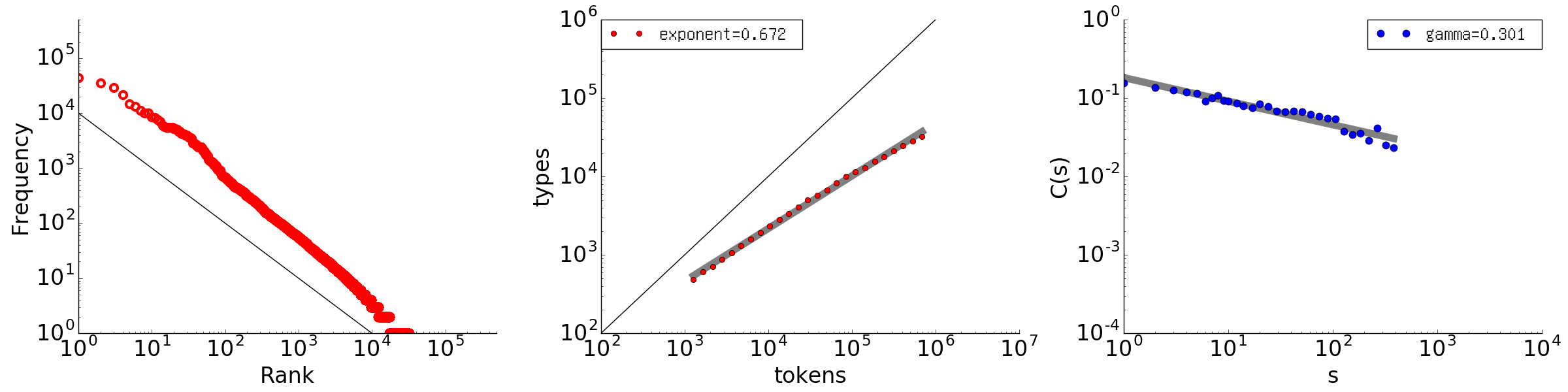
Figure 1: Log-log plots of the rank-frequency distribution, type-token relation, and autocorrelation function for Les Misérables (by V. Hugo (French), number of words $691407$). Left: Rank-frequency distribution, where the x-axis indicates the rank, and the y-axis indicates the frequency. The red points represent the actual data, and the black line indicates a slope of $\xi=1.0$. Middle: Type-token relation, where the x-axis indicates the text size in words, and the y-axis indicates the vocabulary size. The set of red points represents the actual data, along with its fit line in light gray, and the black line indicates a slope of $\zeta=1.0$. The fitted exponent is shown in the upper left corner. Right: Autocorrelation function applied to intervals, where the x-axis indicates the offset $s$, and the y-axis indicates the value of the autocorrelation function $C(s)$ for an interval sequence consisting of one-sixteenth of all the words. The blue points represent the actual data, the thick gray line is the fitted power law, and the slope is shown in the upper right corner.

The focus of this paper is the power law observed for the autocorrelation function when applied to natural language. As an example, the rightmost graph in Figure 1 shows the autocorrelation function applied to the text of Les Misérables. The points are aligned linearly in a log-log plot, so they follow a power law. The correlation is long, in contrast to short-range correlation, in which the points drop much earlier in an exponential way.

There is a history of nearly 25 years of great effort to quantify this long-range correlation underlying text. Since all the existing analysis methods for quantifying long-range memory—i.e., the autocorrelation function that is defined and used later in this section, fluctuation analysis (Kantelhardt et al. 2001) (Kantelhardt 2002), and the older Hurst method (Hurst 1951)—apply only to numerical data, much effort has focused on the question of how best to apply these methods to linguistic (thus, non-numerical) sequences. Previous studies applied one of these methods to a binary sequence based on a certain target word (Ebeling and Pöschel 1994) (Altmann et al. 2012), a word sequence transformed into corresponding frequency ranks (Montemurro 2014), and so on. State-of-the-art approaches use the concept of intervals (Altmann et al. 2009) (Tanaka-Ishii and Bunde 2016), with which a numerical sequence is derived naturally from a linguistic sequence. Note that this transformation into an interval sequence is not arbitrary compared with other transformations, such as the one into a rank sequence. An approach using only interval sequences, however, suffers from the low-frequency problem of rare words, and clear properties cannot be quantified even if they exist. Here, instead, the analysis uses the method proposed in (Tanaka-Ishii and Bunde 2016), which combines interval analysis and extreme value analysis and has been rigorously established, applied, and validated in the statistical physics domain (Lennartz and Bunde 2009). A self-contained summary of the analysis scheme is provided here, and a detailed argument for the method is found in (Tanaka-Ishii and Bunde 2016).

The method basically uses the autocorrelation function to quantify the long-range correlation. Given a numerical sequence $R=r_{1},r_{2},\ldots,r_{M}$, of length $M$, let the mean and standard deviation be $\mu$ and $\sigma$, respectively. Consider the following autocorrelation function:

$$C(s)=\frac{1}{(M-s)\sigma^{2}}\sum_{i=1}^{M-s}(r_{i}-\mu)(r_{i+s}-\mu).$$ (1)

This is a fundamental function to measure the correlation, the similarity of two subsequences of $s$ distance apart: it calculates the statistical co-variance between the original sequence and a sub-sequence starting from the $s$th offset element, standardized by the original variance of $\sigma^{2}$. For every $s$, the value ranges between $-1.0$ and $1.0$, with $C(0)=1.0$ by definition. For a simple random sequence, such as a random binary sequence, the function gives small values fluctuating around zero for any $s$, since the sequence has no correlation with itself. The sequence is judged to be long-range correlated when $C(s)$ decays by a power law, as denoted in the following:

$$C(s)=C(1)s^{-\gamma},s>0.$$ (2)

The particularity of the autocorrelation lies in its long-range nature: two subsequences existing in a sequence remain similar even if $s$ becomes fairly large. Short-term memory, which gives the correlation only for small $s$, shows how the target relies only on local arrangements, in a Markovian way. In contrast, the long-range correlation is considered important precisely because such correlation lasts long. For a natural language sequence, too, $C(s)$ can be calculated, and whether it exhibits power-law decay can be verified. The essential problem lies in the fact that a language sequence is not numerical and thus must be transformed into some numerical sequence.

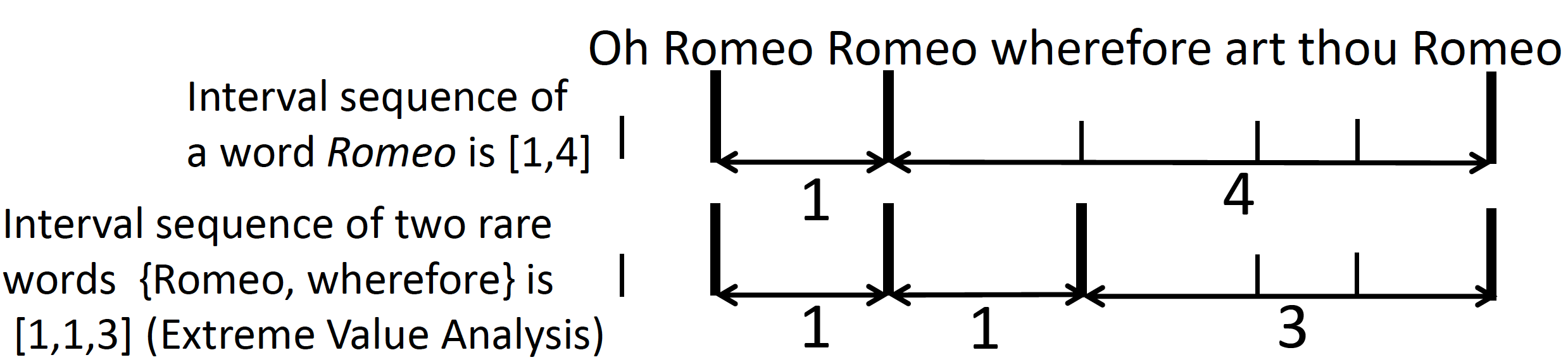
Figure 2: A toy example of interval analysis and extreme value analysis.

The method of (Tanaka-Ishii and Bunde 2016) transforms a word sequence into a numerical sequence by using intervals of rare words. The following example demonstrates how this is done. Consider the target Romeo in the sequence “Oh Romeo Romeo wherefore art thou Romeo,” shown in Figure 2. Romeo, indicated by the thick vertical bar, has a one-word interval between its first and second occurrences, and the third Romeo occurs as the fourth word after the second Romeo. This gives the numerical sequence $[$1, 4$]$ for this clause and the target word Romeo. The target does not have to be one word but could be any element in a set of words. Suppose that the target consisted of two words, the two rarest words in this clause: Romeo, and wherefore. Then, the interval sequence would be $[$1,1,3$]$, since wherefore occurs right after the second Romeo, and the third Romeo occurs as the third word after wherefore. Since rare words occur in such small numbers, consideration of multiple rare words serve to quantify their behavior as an accumulated tendency.

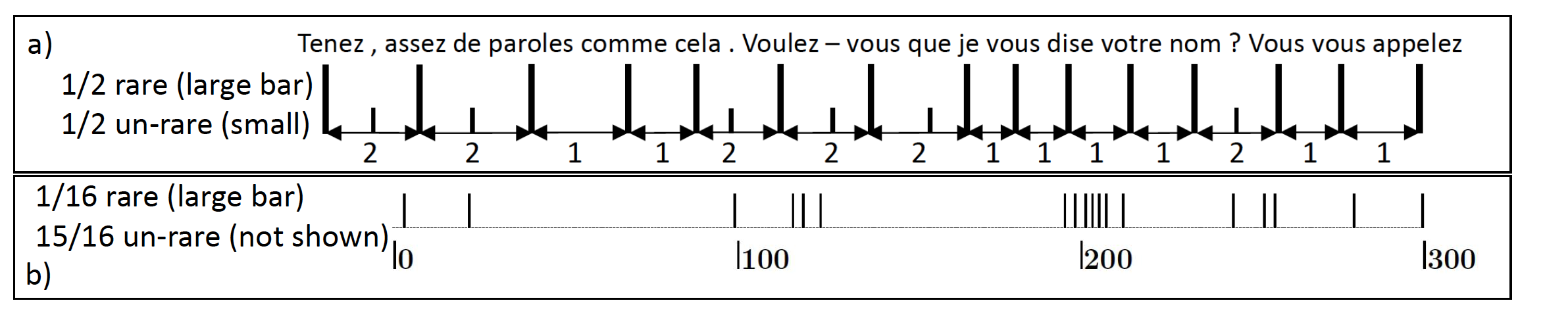
Figure 3: Illustrations of (a) the procedure to acquire an interval sequence and (b) how rare words are clustered in a part of Les Misérables.

Figure 3 illustrates the analysis scheme for a longer sequence. The upper portion (a) shows an example from Les Misérables in which half the words in the text are considered rare (large bars), and the other half, common (small bars). By using the large bars, the text portion is transformed into an interval sequence shown at the bottom as $[$2,2,1,$\ldots$$]$, similarly to the Romeo example in Figure 3. In the bottom portion (b), one sixteenth of all the words, instead of half, are considered rare. The locations of only the large bars are shown for a passage of 300 words starting from the 31096th word in Les Misérables: the bars appear in a clustered manner.

As a summary, the overall procedure is described as follows. Given a numerical sequence of length $M$, the interval length for one $N$th of (rare) words would be $M_{N}\equiv M/N-1$. For the resulting interval sequence $R_{N}=r_{1},r_{2},\ldots,r_{M_{N}}$, let the mean and standard deviation be $\mu_{N}$ and $\sigma_{N}$, respectively. Then the autocorrelation function is calculated for $R_{N}$ with $M_{N}$, $\mu_{N}$, $\sigma_{N}$ replacing $M$, $\mu$, $\sigma$, respectively, in formula (1).

For literary texts, $C(s)$ take positive values forming a power law (Tanaka-Ishii and Bunde 2016). The blue points in the rightmost graph in Figure 1 represent the actual $C(s)$ values in a log-log plot for a sequence of Les Misérables in its entirety. The thick gray line represents the fitted power-law function, which shows that this degree of clustering decays by a power law with exponent $\gamma=0.301$ and a fit error of 0.00158 per point. The fit error reported in this article is the average distance from the fitted line for a point, or in other words, the root of all the accumulated square errors, divided by the number of points. The points were all positive within the chosen range of $s$.

As mentioned previously, the analysis scheme explained above uses extreme value analysis in addition to interval analysis. The method was established within the statistical physics domain, originally for analyzing extreme events with numerical data, such as devastating earthquakes. Analysis schemes using intervals between such rare events always consider rarer events above a threshold (corresponding here to $N$), in order to tackle the low-frequency problem. Various complex systems are known to exhibit long-range correlation (or long-range memory), as reported in the natural sciences and finance, e.g., (Corral 1994: 2005; Bunde et al. 2005; Santhanam and Kantz 2005; Blender et al. 2015; Turcotte 1997; Yamasaki et al. 2007; Bogachev et al. 2007). Rare words in a language sequence should then correspond to extreme events, and the analysis scheme was hence developed as reported in (Tanaka-Ishii and Bunde 2016). That work showed how 10 single-author texts exhibit long-range correlation. Thus, among multiple reports so far, there is abundant evidence arguing that language is long-range correlated in the word arrangement.

Therefore, following that previous work, long-range correlation is reconsidered here through CHILDES data and mathematical generative models. In (Tanaka-Ishii and Bunde 2016), $N$ was varied across $2,4,8,16,32,64$. For large $N$, the interval sequence becomes too short for proper analysis, but for small $N$, it includes words that occur too frequently. To focus on the main point of the article without having too many parameters, $N=16$ is used throughout the remainder.

The main contribution of this paper is to discuss Bayesian models in seeking the reason why such long-range correlation exists. Before proceeding, two other, more common power laws are introduced because they are necessary for the later discussion in §4. The leftmost graph in Figure 1 shows the log-log rank-frequency distribution for Les Misérables, which demonstrates a power-law relationship between the frequency rank and frequency, i.e., Zipf’s law. Given word rank $u$ and frequency $F(u)$ for a word of rank $u$, Zipf’s law suggests the following proportionality formula:

$$F(u)\propto u^{-\xi},\ \ \hskip 8.53581pt\xi\approx 1.0.$$ (3)

As shown here for Les Misérables, the plot typically follows formula (3) only very approximately. A skew or bias, such as the convex tendency to the upper right, often appears, as will be seen for the CHILDES corpus in the following section. There have been discussions on how to improve the Zipf model by incorporating such bias (Mandelbrot 1952) (Mandelbrot 1965) (Montemuro 2001) (Deng et al. 2014) altmanprx. To the best of the author’s knowledge, however, mathematical model fully explains the bias is still under debate.

The middle graph in Figure 1 shows the type-token relation based on another power law, usually referred to as Heaps’ Law, indicating the growth rate of the vocabulary size with respect to text length. Given vocabulary size $V(m)$ for a text of length $m$, Heaps’ law is as follows:

$$V(m)\propto m^{\zeta},\ \ \hskip 8.53581pt\zeta<1.0.$$ (4)

This feature was known even before (Heaps 1978), as published in (Herdan 1964) and (Guiraud 1954). In the graph, the black line represents an exponent of 1.0. As seen here, for Les Misérables, $\zeta=0.672$, much smaller than 1.0; indeed, the growth rate for natural language is below 1.0.

3 Autocorrelation Functions for Childhood Language

Using the method introduced in the previous section, this section introduces a kind of data, which has never been considered in the context of long-range correlation: childhood language data from the CHILDES corpus. In contrast to the previous work on single-author texts, these data concern utterances (speech). Furthermore, the data are chronologically ordered, thus showing the development of a child’s linguistic capability.

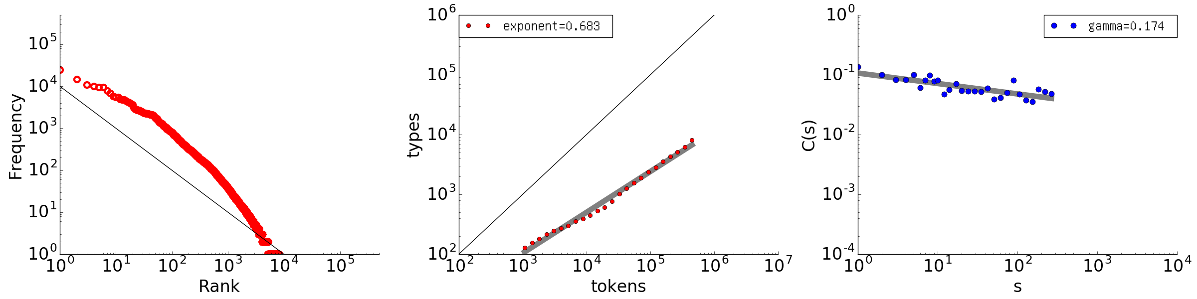
Figure 4: Rank-frequency distribution, type-token relation, and autocorrelation function for the Thomas data set (103762 words).

The first example is Thomas in English, which is the longest data set in CHILDES. Figure 4 shows the rank-frequency distribution, type-token relation, and autocorrelation function for Thomas’ utterances, similarly to Figure 1.

The autocorrelation function (right) has a surprisingly tight power law, thus indicating long-range correlation. Since a child’s utterances are linguistically under development, this result is not trivial. The slope is smaller than that of the literary text shown in Figure 1. None of the calculated $C(s)$ values were negative, and the fit error was 0.00255 per point.

As for the rank-frequency distribution (left), the overall slope is larger than 1.0 and the plot has a clear convex tendency, as compared with the black line representing a slope of 1.0. Such convex tendency of the rank-frequency distribution has been reported elsewhere, such as for single-author collections (Montemuro 2001) or Chinese characters (Deng et al. 2014), but the convexity here seems different from both of those cases. This convex tendency suggests, rather, that Thomas generated utterances using more frequent words, especially the top 100 words.

Lastly, the middle graph shows the type-token relation. As compared with Les Misérables, the vocabulary growth is less stable and slightly steeper, with an exponent of $\zeta=0.683$.

The 10 longest CHILDES data sets were selected, and these included utterances in different languages. The utterances were carefully separated by speaker, and only those by children were used. Moreover, the CHILDES codes for unknown words were removed. Figure 5 shows the autocorrelation function results for Thomas and the other nine children. Although not always as tight as in Thomas’s case, the power law does hold in every case. Except for a single point at $s=10$ for Ris, all calculated $C(s)$ values are positive and aligned almost linearly. Moreover, the power law holds more tightly for the larger data sets.

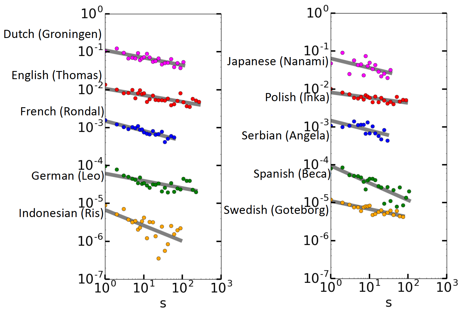
Figure 5: Autocorrelation functions for the 10 children. For the sake of vertical placement, the $C(s)$ values for the $z$th data set from the top are multiplied by $1/10^{z-1}$ in each graph.

4 Generative Language Models

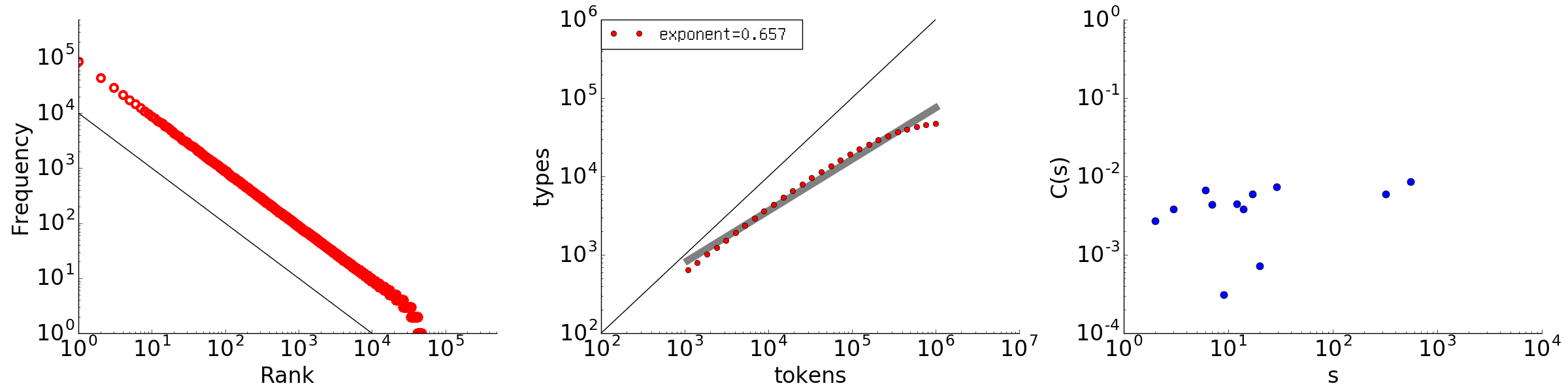
Figure 6: Rank-frequency distribution, type-token relation, and autocorrelation function for a randomly generated sequence that follows a Zipf distribution (one million words with a vocabulary size of 50000).

The autocorrelative characteristic reported here for children’s utterances and in many previous works for natural language texts does not hold for simple random data. To demonstrate this, three examples are provided. The first example is a randomized word set whose rank-frequency sequence strictly follows a Zipf distribution. Figure 6 shows graphs of the rank-frequency distribution, type-token relation, and autocorrelation function for this sequence, with a length of one million words and a vocabulary size of 50000 words.

The leftmost graph does exhibit a power law with the exponent $-1.0$, but the rightmost graph shows that the long-range correlation is completely destroyed. Many $C(s)$ values are negative and thus not shown here because the plot is log-log. As noted before, for random data the autocorrelation function fluctuates around 0. Approximately half the values become negative and thus disappear from the figure, leaving a sparse set of plotted points, exactly as observed here.

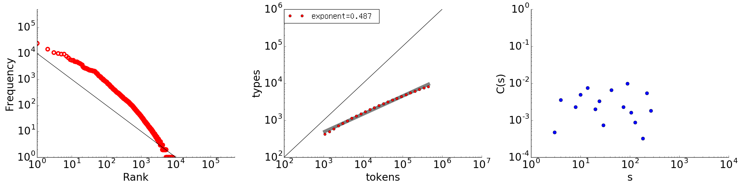
Figure 7: Rank-frequency distribution, type-token relation, and autocorrelation function for the Thomas data set randomly shuffled at the word level.

A second example was obtained by shuffling Thomas’s utterances at the word level. Random shuffling destroys the original intervals between words in the Thomas data set. Figure 7 shows the analysis results, in which the autocorrelation function has become random, whereas the rank-frequency distribution and type-token relation remain the same as the original results shown in Figure 4.

Figure 8: Rank-frequency distribution, type-token relation, and autocorrelation function for a sequence randomly generated from bigram (1st-order Markov) models of Les Misérables (one million words).

The third example is a Markov sequence generated using bigrams obtained from Les Misérables. The random sequence was generated from the bigrams according to the probabilities recorded in a word transition matrix. Figure 8 shows the analysis results, with the rightmost graph indicating that the autocorrelation function does not exhibit any memory.

Long-range correlation therefore does not hold for such simple random sequences. At the same time, given that long-range memory holds for the CHILDES data, it should be natural to consider that some simple mechanism underlies language production. In early childhood speech, utterances are still lacking in full vocabulary, ungrammatical, and full of mistakes. Therefore, the long-range correlation of such speech must be based on a simple mechanism other than linguistic features such as grammar that we generally consider.

The problem with all the findings related to power laws underlying the statistical physics domain is that even though, as mentioned before, the method has been effective in analyzing natural sciences and finance, the exact reason why such power laws hold remains unknown. This applies to long-range correlation, as well: “rare words tend to cluster” is only one simplistic way to express a limited aspect of the phenomenon. As mentioned before, however, the phenomenon is more complex and has some relation to the scale-free property underlying language.

In the case of Zipf’s law, Mandelbrot mathematically proved that it holds by optimizing the communication efficiency (Mandelbrot 1952)(Mandelbrot 1965). It is unknown how this optimization theory could relate to long-range correlation. Moreover, it is not obvious whether an infant child would optimize every word of an utterance. It would be more natural to consider that a child learns how to act in choosing a word, and that this action, in fact, is mathematically bound so as to be optimal. One possible approach to understand what’s behind such an act would be to consider the behavior of mathematical models of language with respect to power laws. Roughly, at least four representative families of mathematical processes have been considered as language models: Markov models, Poisson processes Church and Gale (1995) or renewal processes Altmann et al. (2009), neural languages models, and recent Bayesian models. The first two models require a predefined vocabulary size, so without further modification of these models, they could not be applied to confirm either Zipf’s or Heaps’ law. Neural language models have been successful in language applications, but has been reported recently that they do not exhibit long range correlation Takahashi and Kumiko Tanaka-Ishii (2018).

The rest of this paper therefore focuses on Bayesian models, which naturally accommodate infinite vocabulary growth. In all the generative models presented hereafter, the model generates elements one after another, either by introducing a new word or by reusing a previous element. Let $K_{t}$ be the number of kinds of elements (vocabulary size) at time $t$, and let $S_{t,i}$ be the frequency of elements of kind $i$ occurring until $t$. At $t=0$, all models presented hereafter start with the following status:

$$K_{0}=1,\hskip 8.53581ptS_{0,1}=1,\hskip 8.53581ptS_{0,i}=0,\hskip 8.53581pti\in\mathbb{Z}_{>1}.$$

The most fundamental model is the Simon model (Simon 1955) (Mitzenmacher 2003). This model, described colloquially as “the rich get richer,” is used for a variety of natural and artificial phenomena. A similar model in complex network systems is the Barabási-Albert model (Barabasi and Reka 1999). For $t>0$, given a constant $0<\alpha<1$, an element is generated at time $t+1$ with the following probabilities:

$$\displaystyle P(K_{t+1}=K_{t}+1,S_{t+1,j}=S_{t,j},j\in\mathbb{Z}_{\geq 1}\backslash\{K_{t}+1\},S_{t+1,K_{t}+1}=1) = \alpha,$$

$$P(K_{t+1}=K_{t},S_{t+1,i}=S_{t,i}+1,S_{t+1,j}=S_{t,j},j\in\mathbb{Z}_{\geq 1}\backslash\{i\}) = (1-\alpha)\frac{S_{t,i}}{t},i=1,\ \ \ldots,K_{t}.$$

Note that the first definition gives the case when a new word is introduced, and the second gives the case when a previous word is sampled. The scheme can thus be described as follows: with constant probability $\alpha$, a new, unseen element is generated; and with the remaining probability $1-\alpha$, an element that has already occurred is selected according to the frequency distribution in the past. Suppose, for example, that the previously generated sequence is $X$=$[$‘x’, ‘y’, ‘x’, ‘z’, ‘x’, ‘z’$]$. Then the next element will be a new element with probability $\alpha$, or ‘x’, ‘y’, or ‘z’ with probability $3(1-\alpha)/6$, $(1-\alpha)/6$, or $2(1-\alpha)/6)$, respectively. It is trivial to understand that this reuse of previous elements is equivalent to a uniform sample from the past sequence, i.e., by considering that all past elements occurred equally under a uniform distribution. In this example, uniform sampling entails picking one element randomly from $X$=$[$‘x’, ‘y’, ‘x’, ‘z’, ‘x’, ‘z’$]$.

It has been mathematically proven that the rank-frequency distribution of a sequence generated with the Simon model roughly follows a power law, independently of the value of $\alpha$ (Mitzenmacher 2003). Since the vocabulary introduction rate is constant, it is trivial to see that the type-token ratio also has the exponent $1.0$.

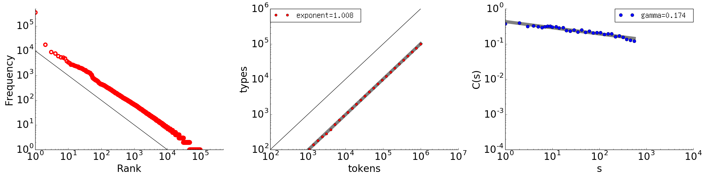
Figure 9: Rank-frequency distribution, type-token relation, and autocorrelation function for a one-million-element sequence generated with the Simon model, where $\alpha=0.10$.

To investigate the Simon model, a sequence of one million elements with $\alpha=0.10$ was generated, and its rank-frequency distribution, type-token relation, and autocorrelation function were obtained. The autocorrelation function was calculated according to the scheme explained in §2, since a new element introduced in this scheme can be anything, even a non-numerical element.

Figure 9 shows the results. The first two graphs agree with the theory by giving exponents of $-1.0$ and $1.0$, respectively. As for the autocorrelation function, surprisingly, long-range memory is clearly present. The slope is $\gamma=0.174$, which is coincidentally the same as that for the Thomas data set. None of the $C(s)$ values is negative, and the fit to the slope is very tight, with a fit error of 0.00369.

To examine the parameter dependence, 10 sequences for each of $\alpha={0.1,0.2,0.3,0.4}$ were generated, and the autocorrelation function was obtained for each. The results included no negative $C(s)$ values. For each $\alpha$, the respective mean values of $\gamma$ were 0.156, 0.133, 0.118, and 0.095, with small standard deviations of 0.019, 0.018, 0.011, and 0.013, respectively. Thus, the slope decreased with increasing $\alpha$. The average fit error obtained via the square error across all 40 sequences was 0.00366 per point.

The Simon model has two known problems, however, as a language model. The first is that the vocabulary growth (proven to have exponent 1.0) is too fast. Indeed, such fast vocabulary growth is very unlikely in natural language production. The second problem is that the model cannot handle the convexity underlying a rank-frequency distribution, as observed especially for the Thomas data set (Figure 4). Such convexity has been reported elsewhere, as noted before.

Another Bayesian model called the Pitman-Yor model (Pitman 2006) solves these two problems. Using the same mathematical notation as before, and given two constants $0\leq a<1$ and $0\leq b$, the following generative process is applied for $t>0$ at time $t+1$ with the following probabilities:

$$P(K_{t+1}=K_{t}+1,S_{t+1,j}=S_{t,j},j\in\mathbb{Z}_{\geq 1}\backslash\{K_{t}+1\},S_{t+1,K_{t}+1}=1) = \frac{aK_{t}+b}{t+b},$$

$$P(K_{t+1}=K_{t},S_{t+1,i}=S_{t,i}+1,S_{t+1,j}=S_{t,j},j\in\mathbb{Z}_{\geq 1}\backslash\{i\}) = \frac{S_{t,i}-a}{t+b},i=1,\ \ \ldots,K_{t}.$$

As with the Simon model, the first line defines the introduction rate for new elements. It decreases with the length of the sequence, $t$, yet is linear in the vocabulary size $K_{t}$ according to the strength $a$. This amount is generated as a sum of taking every element kind $i=1,\ldots,K_{t}$ by subtracting $a$ from frequency $S_{t,i}$, which appears in the numerator of the second definition above. Apart from this, the parameter $b$ controls the convex trend (Pitman 2006) (Teh 2006) often seen in rank-frequency distributions. When $a=0$, this model reduces to the Chinese restaurant process (Goldwater et al. 2009), which has been applied widely in the language engineering domain.

Mathematically, the parameter $a$ in the Pitman-Yor model almost equals the value of the exponent of the type-token relation, $\zeta$, which describes the vocabulary growth speed, provided that $b$ is small and Heaps’ law holds (Appendix A). According to empirical verification, even for a large $b=10000$, $\zeta$ only differed from $a$ by a maximum of 0.1. Given this, $a=0.68$ was chosen for the remaining Pitman-Yor models presented in this article, a value somewhat in the middle of $\zeta=0.683$ for the Thomas data set and $\zeta=0.672$ for Les Miserables.

For generation of one million elements by a Pitman-Yor process with $a=0.68$ and $b=0.80$, Figure 10 shows the three resulting graphs. Agreeing with theory, the middle graph showing the type-token relation has a slope reasonably close to 0.68. As for the leftmost graph showing the rank-frequency distribution, with $b=0.80$ a slight convex tendency appears, but with a larger $b\geq 100$, the convex tendency would clearly be present. In the rightmost figure, however, the power law of particular interest here, for the autocorrelation function, has disappeared. Although the change from the Simon model is subtle, with respect to the value of $a$, the sequence does not exhibit any arrangement underlying natural language.

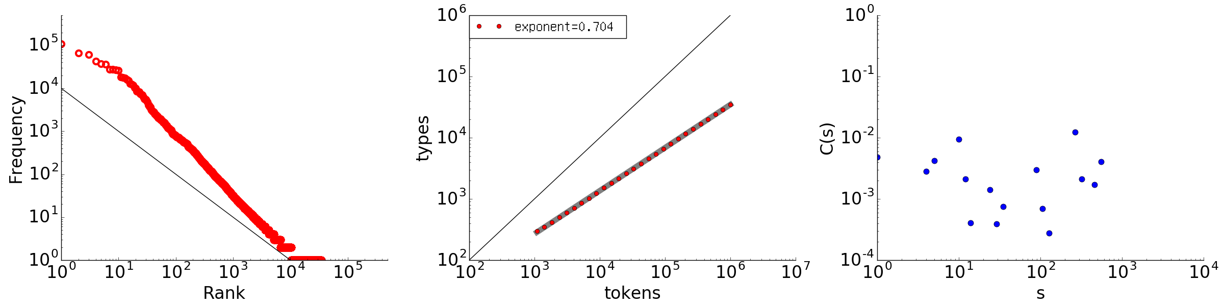
Figure 10: Rank-frequency distribution, type-token relation, and autocorrelation for a sequence of one million elements generated by a Pitman-Yor model with $a=0.68$ and $b=0.80$.

Since this result could be due to the parameter setting, all possible combinations of $a=\{0.0,0.1,0.2,\dots,0.9\}$ (10 values) and $b=\{0.0,0.1,0.2,\ldots,1.0,10.0,100.0,1000.0,10000.0\}$ (15 values) were considered. For every pair $(a,b)$ out of these 150 possibilities, a sequence of one million elements was generated and examined for long-range correlation. If any $C(s)$ value for $s<10$ was negative, then long-range memory was judged not to hold. This criterion is somewhat loose, because it considers long-range correlation to hold even when the points are scattered and not exhibiting power-law behavior, as long as they are still positive. Even with this loose criterion, however, none of the sequences had long-range correlation. When $a$ is too small, the rate of introducing new words becomes too weak. Even when there are sufficient new words, the arrangement seems qualitatively different from the case of the Simon model.

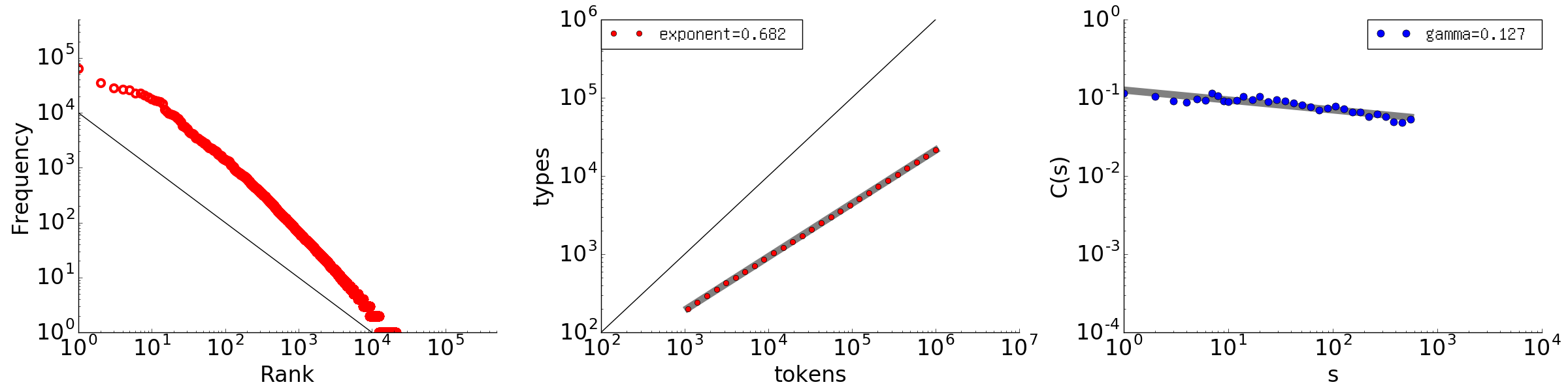
Figure 11: Rank-frequency distribution, type-token relation, and autocorrelation for a sequence of one million elements generated by the proposed conjunct model with $a=0.68$ and $b=0.80$.

We have now seen that the Simon model exhibits a bad type-token relation but a good autocorrelation, while the opposite is true for the Pitman-Yor model. Since long-range correlation is due to the arrangement of frequent words and rare words, a natural approach is to test the following conjunct generative model for $t>0$ at time $t+1$ with the following probabilities:

$$P(K_{t+1}=K_{t}+1,S_{t+1,j}=S_{t,j},j\in\mathbb{Z}_{\geq 1}\backslash\{K_{t}+1\},S_{t+1,K_{t}+1}=1) = \eta,\ \ \ where\ \ \eta=\frac{aK_{t}+b}{t+b},$$

$$P(K_{t+1}=K_{t},S_{t+1,i}=S_{t,i}+1,S_{t+1,j}=S_{t,j},j\in\mathbb{Z}_{\geq 1}\backslash\{i\}) = (1-\eta)\frac{S_{t,i}}{t},i=1,\ \ \ldots,K_{t}.$$

This mixed model introduces new words with a probability $\eta$ equal to that of the Pitman-Yor model, so the first line is exactly the same as in the definition of that model. As for sampling, with probability $1-\eta$ a previous element is introduced in proportion to the frequencies of the elements. In other words, the conjunct model achieves uniform sampling, as in the Simon model, by replacing that model’s $\alpha$ with $\eta$.

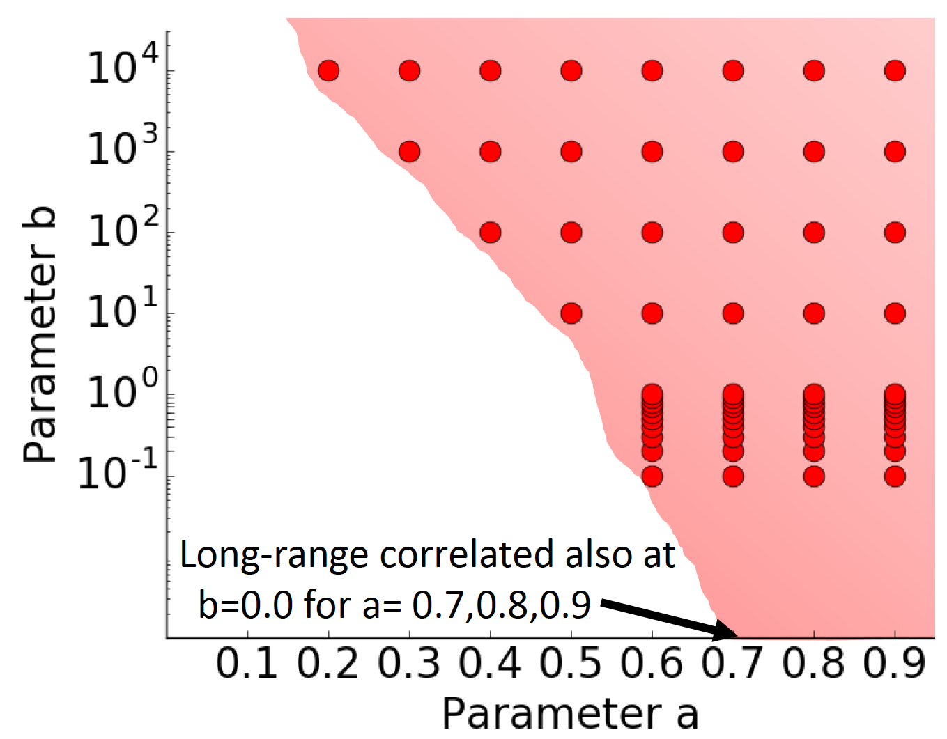
Figure 12: Pairs of parameters $a$ and $b$ for which a sequence generated by the conjunct model exhibits long-range correlation. The red dots represent the experimental results, while the interpolated area of long-range correlation was manually shaded red.

Figure 11 shows the behavior of a sequence generated by the conjunct model with $a=0.68$ and $b=0.80$. The model clearly exhibits the desired vocabulary growth while maintaining its long-range correlation. The $\gamma$ exponent decreases to 0.127, with a fit error of 0.00162.

To examine the parameter dependence, again all possible combinations of 10 values of $a=\{0.0,0.1,0.2,\dots,0.9\}$ with $b=\{0.0,0.1,0.2,\ldots,0.9,1.0,10.0,100.0,1000.0,10000.0\}$ (15 values) were again considered. For every pair $(a,b)$, a sequence of one million elements was generated 10 times and examined for long-range correlation. Figure 12 shows all the pairs of values for which long-range correlation was observed. When $a$ is too small, the rate of introducing new words becomes too small and gives no correlation. For a sufficiently large $a$ and a value of $b$ that depends on $a$, on the other hand, long-range correlation is observed.

The variance of the obtained exponent $\gamma$ for the autocorrelation function was almost the same for small $b$ below 1.0. For example, for $a=0.68$ the average $\gamma$ was 0.126 with a standard deviation of 0.0318 and fit error per point of 0.0013. For larger $b$, $\gamma$ tended to be smaller. For other $a$ values, as well, the $\gamma$ values were not as steep as 0.2.

5 Discussion

The findings reported in this article lead to two main points. First, the findings raise the question of the Pitman-Yor model’s validity as a language model. Pitman-Yor models have been used because they nicely model the rank-frequency distribution and the growth rate of natural language. However, the Pitman-Yor model is not long range correlated, different from natural language. Although the current work does not invalidate the usefulness of Pitman-Yor models for language engineering (since they are effective), the long-range correlation behavior does reveal a difference between the nature of language and a Pitman-Yor model. This could be a factor for consideration in future scientific research on language.

Second, this work reveals that among possible mathematical language models considered so far, those with uniform sampling generated strong long-range correlation (i.e., the Simon model and the conjunct model developed at the end of the previous section). Given how simple uniform sampling is, however, the findings could suggest that natural language has some connection with uniform sampling. In fact, long-range correlation is present in music, as well (Appendix B), which is another human resource, similar to language. Therefore, the human faculty to generate linguistic-related time series might have a fundamental structure with some relation to a very simple procedure, with uniform sampling as one possibility.

Without noting, however, uniform sampling only by itself is limited as a language model. In addition to the lack of linguistic grammatical features, the Simon model and its extensions exhibit different nature at the beginning part and later part of the sample: this is different from language, where a sample from any location of the data is long range correlated. Mathematical generative processes that satisfy all the stylized facts of languages would aid to clarify what kind of process language is, and to this end, the proposed conjunct model could be yet another starting point towards a better language model. The conjunct model currently has two differences from actual natural language. The first is the exponent $\gamma$, which is larger for both literature and the CHILDES data, sometimes exceeding 0.3, but remains below around 0.15 for the conjunct model. Second, the rank-frequency distribution is convex for large $b$ in the conjunct model, but such large $b$ makes $\gamma$ even smaller. Therefore, the conjunct model must be modified to fill this gap. This would require more exhaustive knowledge of long-range memory in natural language, and the model would have to integrate more complex schemes that possibly introduce n-grams or grammar models.

6 Conclusion

This article has investigated the long-range correlation underlying the autocorrelation function with CHILDES data and Bayesian models by using an analysis method for non-numerical time series, which was borrowed from the statistical physics domain. After first overviewing how long-range correlation phenomena have been reported for different kinds of natural language texts, they were also verified to occur for children’s utterances.

To find a reason for this shared feature, we investigated three generative models: the Simon model, the Pitman-Yor model, and a conjunct model integrating both. The three models share a common scheme of introducing a new element with some probability and otherwise sampling from the previous elements. The Simon model exhibits outstanding long-range correlation, but it deviates from natural language texts by causing the vocabulary to grow too fast. In contrast, the Pitman-Yor model exhibits no long-range correlation, despite having an appropriate vocabulary growth rate. Therefore, the conjunct model uses the Pitman-Yor introduction rate for new vocabulary but samples from the past through uniform sampling, like the Simon model. This conjunct model produces long-range correlation while maintaining a growth rate similar to that of natural language text.

The fact that the Pitman-Yor model does not exhibit long-range correlation raises the question of the Pitman-Yor model’s validity as a natural language model. Since the mathematical generative models among Simon kind that exhibited long-range correlation are based on uniform sampling, we may conjecture that there could be some relation between natural language and uniform sampling. The findings in this article could provide another direction towards better future language models.

Appendix A

This appendix explains why $a\approx\zeta$. At time $t$, the number of words introduced into the sequence is

$$K_{t}=\int_{0}^{t}\frac{aK_{t}+b}{t+b}.$$ (5)

Assuming that $b$ is sufficiently small and $K_{t}=t^{\zeta}$,

$$\displaystyle\int_{0}^{t}\frac{at^{\zeta}+b}{t+b} \approx \int_{0}^{t}at^{\zeta-1}$$ (6)

$$= \frac{a}{\zeta}t^{\zeta},$$ (7)

and since this must equal $K_{t}$, $a=\zeta$. Empirically, this was almost always the case for $b$ up to around 1.0. For larger $b$, $\zeta$ became larger than $a$: when $b=10000$, for example, $\zeta$ was larger than $a$ by 1.0, at most.

Appendix B

This Appendix shows the long range correlation of 10 long classical music pieces (Figure 13). Original data was in MIDI format and they are pre-processed. The headers and footers were eliminated and so that the data contain only the musical part, including pause indications. Every tune played by different instrument kind is separated and concatenated As far as these 10 pieces, the long range correlation can be considered as to hold. Previous work on also reports how long-range correlation holds in skilled piano playRuiz et al. (2014).

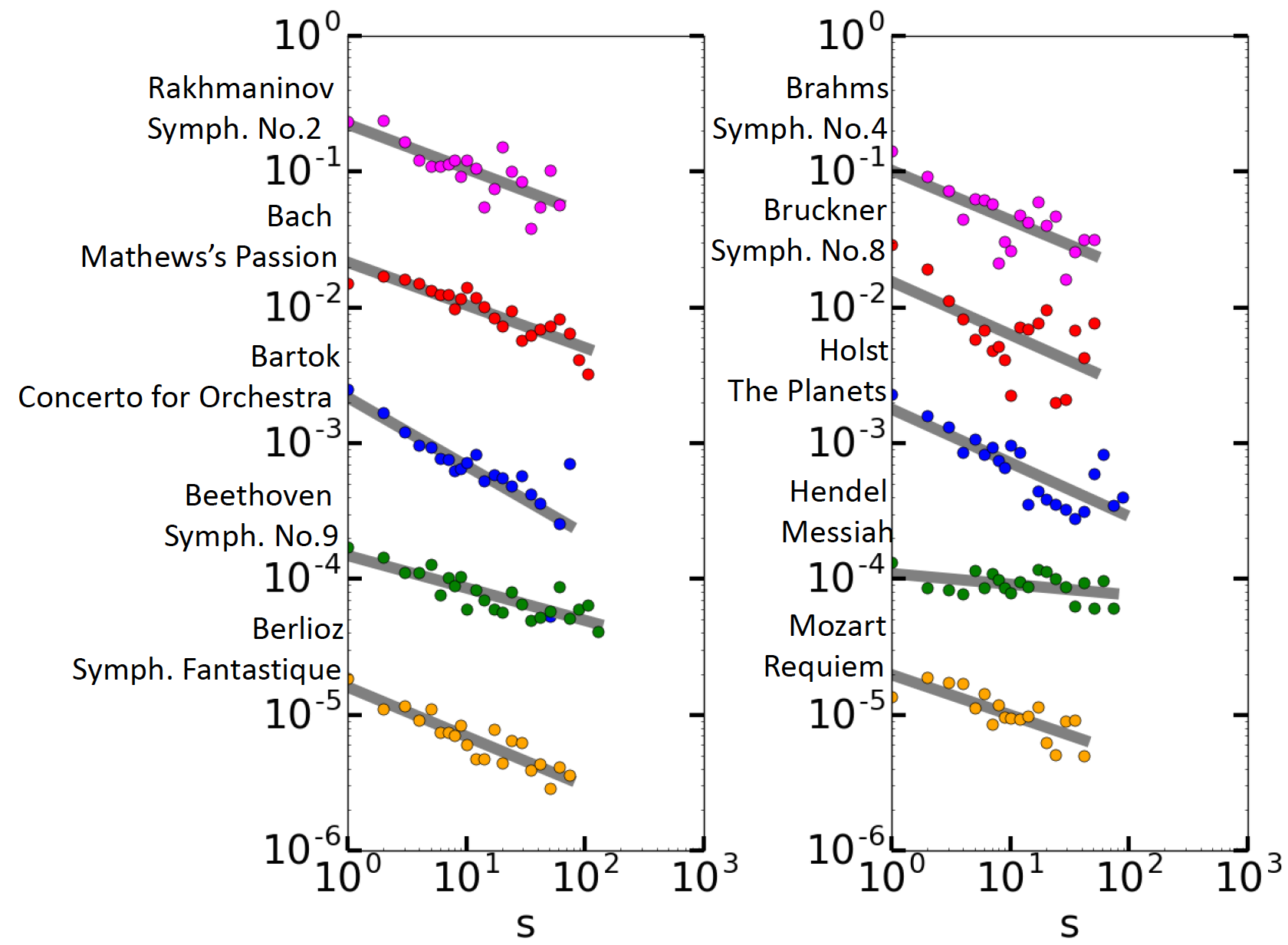
Figure 13: Long range correlation of 10 long classical music pieces. For the sake of vertical placement, the C(s) values for the zth data set from the top are multiplied by $1/10^{z-1}$ in each graph.

References

- Altmann et al. (2009) Altmann, E.G. , Pierrehumbert, J.B. , and Motter, E.A. (2009). Beyond word frequency: Bursts, lulls, and scaling in the temporal distributions of words.
- Altmann et al. (2012) Altmann, E.G. , Cristadoro, G. , and Esposti, M.D. (2012). On the origin of long-range correlations in texts. Proceedings of the National Acaddemy of Sciences, 109, 11582–11587.
- Barabasi and Reka (1999) Barabasi, A.-L. and Reka, A. (1999). Emergence of scaling in random networks. Science, pages 509–612. 286.
- Bedia et al. (2014) Bedia, M.G. , Aguilera, M. , Gomez, T. , Larrode, D.G. , and Seron, F. (2014). Quantifying long-range correlations and 1/f patterns in a minimal experiment of social interaction. Frontiers in Psychology. https://doi.org/10.3389/fpsyg.2014.01281.
- Blender et al. (2015) Blender, R. , Raible, C. , and Lunkeit, F. (2015). Non-exponential return time distributions for vorticity extremes explained by fractional poisson processes. Quarterly Journal of the Royal Meteorology Society, 141, 249–257.
- Bogachev et al. (2007) Bogachev, M.I. , Eichner, J.F. , and Bunde, A. (2007). Effect of nonlinear correlations on the statistics of return intervals in multifractal data sets. Physical Review Letters, 99(240601).
- Bunde et al. (2005) Bunde, A. , Eichner, J. , Havlin, S. , and Kantelhardt, J.W. (2005). Long-term memory: A natural mechanism for the clustering of extreme events and anomalous residual times in climate records. Physical Review Letters, 94(048701).
- Chater and Oaksford (2008) Chater, N. and Oaksford, M. (2008). The Probabilistic Mind: Prospects for Bayesian Cognitive Science. Oxford University Press.
- Church and Gale (1995) Church, K.W. and Gale, W.A. (1995). Poisson mixtures. Natural Language Engineering, pages 163–190.
- Corral (1994) Corral, A. (1994). Long-term clustering, scaling, and universality in the temporal occurrences of earthquakes. Physical Review Letters, 92(108501).
- Corral (2005) Corral, A. (2005). Renomalization-group transformations and correlations of seismicity. Physical Review Letters, 95(028501).
- Deng et al. (2014) Deng, W. , Allahverdyan, E. , and Wang, Q. A. (2014). Rank-frequency relation for chinese characters. The European Physical Journal B. 87:47.
- Ebeling and Pöschel (1994) Ebeling, W. and Pöschel, T. (1994). Entropy and long-range correlations in literary english. Europhys. Letters, 26, 241–246.
- Goldwater et al. (2009) Goldwater, S. , Griffiths, Thomas L. , and Johnson, M. (2009). A baysian framework for word segmentation: Exploring the effects of context. Cognition, pages 21–54.
- Goldwater et al. (2011) Goldwater, S. , Griffiths, Thomas L. , and Johnson, M. (2011). Producing power-law distributions and damping word frequencies with two-stage language models. Journal of Machine Learning Research, pages 2335–2382.
- Guiraud (1954) Guiraud, H. (1954). Les Charactères Statistique du Vocabulaire. Universitaires de France Press.
- Heaps (1978) Heaps, H. S. (1978). Information retrieval: Computational and theoretical aspects, academic press. page 206–208.
- Herdan (1964) Herdan, G. (1964). Quantitative Linguistics. Butterworths.
- Hurst (1951) Hurst, H. E. (1951). Long-term storage capacity of reservoirs. Transactions of the American Society of Civil Engineers, 116, 770–808.
- Kantelhardt et al. (2001) Kantelhardt, J. W. , Koscielny-Bunde, E. , Rego, H. H. A. , Havlin, S. , and Bunde, A. (2001). Detecting long-range correlations with detrended fluctuation analysis. Physica A, 295, 441–454.
- Kantelhardt (2002) Kantelhardt, J. W. et al. (2002). Multifractal detrended fluctuation analysis of non-stationary time series. Physica A, 316, 87.
- Lee and Wagenmakers (2014) Lee, D. M. and Wagenmakers, E.-J. (2014). Bayesian Cognitive Modeling: A Practical Course. Cambridge University Press.
- Lennartz and Bunde (2009) Lennartz, S. and Bunde, A. (2009). Eliminating finite-size effects and detecting the amount of white noise in short records with long-term memory. Physical Review E, 79(066101).
- Mandelbrot (1952) Mandelbrot, B. (1952). An informational theory of the statistical structure of language. Proceedings of Symposium of Applications of Communication theory, pages 486–500.
- Mandelbrot (1965) Mandelbrot, B. (1965). Information theory and psycholinguistics. Basic Books.
- Mitzenmacher (2003) Mitzenmacher, M. (2003). A brief history of generative models for power law and lognormal distributions. Internet Mathematics, 1(2), 226–251.
- Montemuro (2001) Montemuro, M.A. (2001). Beyond the zipf-mandelbrot law in quantitative linguistics. Physica A: Statistical Mechanics and its Applications, 300, 567–678.
- Montemurro (2014) Montemurro, M.A. (2014). Quantifying the information in the long-range order of words: Semantic structures and universal linguistic constraints. Cortex, 55, 5–16.
- Pitman (2006) Pitman, J. (2006). Combinatorial Stochastic Processes. Springer.
- Ruiz et al. (2014) Ruiz, M.H. , Hong, S.B. , Hennig, H. , Altenmüller, E. , and Kühn, A.A. (2014). Long-range correlation properties in timing of skilled piano performance: the influence of auditory feedback and deep brain stimulation. Frontiers in Psychology. https://doi.org/10.3389/fpsyg.2014.01030.
- Santhanam and Kantz (2005) Santhanam, M. and Kantz, H. (2005). Long-range correlations and rare events in boundary layer wind fields. Physica A, 345, 713–721.
- Serrano et al. (2009) Serrano, M.A. , Flammini, A. , and Menczer, F. (2009). Modeling statistical properties of written text. PLOS ONE. http://journals.plos.org/plosone/article?id=10.1371/journal.pone.0005372.
- Simon (1955) Simon, H.A. (1955). On a class of skew distribution functions. Biometrika, 42(3/4), 425–440.
- Takahashi and Kumiko Tanaka-Ishii (2018) Takahashi, Shuntaro and Kumiko Tanaka-Ishii (2018). Do neural nets learn statistical laws behind natural langauge? PLoS One. https://arxiv.org/abs/1707.04848.
- Tanaka-Ishii and Bunde (2016) Tanaka-Ishii, K. and Bunde, A. (2016). Long-range memory in literary texts: On the universal clustering of the rare words. PLOS One. http://journals.plos.org/plosone/article?id=10.1371/journal.pone.0164658.
- Teh (2006) Teh, Y.W. (2006). A hierarchical bayesian language model based on pitman-yor processes. In Annual Conference on Computational Linguistics, pages 985–992.
- Turcotte (1997) Turcotte, D.L. (1997). Fractals and Chaos in Geology and Geophysics. Cambridge University Press.
- van Emde Boas (2004) van Emde Boas, E. (2004). Clusters of Hapax Legomena: An examination of hapax-dense passage in the Iliad. Universiteit van Amsterdam. XXX thesis.
- Yamasaki et al. (2007) Yamasaki, K. , Muchnik, L. , Havlin, S. , Bunde, A. , and Stanley, H.E. (2007). Scaling and memory in volatility return intervals in financial markets. Proceedings of the National Acaddemy of Sciences, 102, 9424–9428.