How proper are Bayesian models in the astronomical literature?

Abstract

The well-known Bayes theorem assumes that a posterior distribution is a probability distribution. However, the posterior distribution may no longer be a probability distribution if an improper prior distribution (non-probability measure) such as an unbounded uniform prior is used. Improper priors are often used in the astronomical literature to reflect a lack of prior knowledge, but checking whether the resulting posterior is a probability distribution is sometimes neglected. It turns out that black23 articles out of 75 articles (black30.7%) published online in two renowned astronomy journals (ApJ and MNRAS) between Jan 1, 2017 and Oct 15, 2017 make use of Bayesian analyses without rigorously establishing posterior propriety. A disturbing aspect is that a Gibbs-type Markov chain Monte Carlo (MCMC) method can produce a seemingly reasonable posterior sample even when the posterior is not a probability distribution (Hobert and Casella,, 1996). In such cases, researchers may erroneously make probabilistic inferences without noticing that the MCMC sample is from a non-blackexisting probability distribution. We review why checking posterior propriety is fundamental in Bayesian analysesblack, and discuss how blackto set up scientifically motivated proper priors.

1 Introduction

A Bayesian model is uniquely determined by two components: (i) a likelihood function of unknown parameters $\boldsymbol{\theta}$ given the data $\boldsymbol{y}$ denoted by $L(\boldsymbol{\theta};\boldsymbol{y})$, which is proportional to a conditional probability density $f(\boldsymbol{y}\mid\boldsymbol{\theta})$ of a sampling distribution, and (ii) a joint prior density, $p(\boldsymbol{\theta})$. Using the fundamental Bayes theorem black(see Appendix A for details), we can derive the posterior density of $\boldsymbol{\theta}$ as follows:

$$\pi(\boldsymbol{\theta}\mid\boldsymbol{y})=\frac{f(\boldsymbol{y}\mid\boldsymbol{\theta})p(\boldsymbol{\theta})}{\int f(\boldsymbol{y}\mid\boldsymbol{\theta})p(\boldsymbol{\theta})d\boldsymbol{\theta}}=\frac{L(\boldsymbol{\theta};\boldsymbol{y})p(\boldsymbol{\theta})}{\int L(\boldsymbol{\theta};\boldsymbol{y})p(\boldsymbol{\theta})d\boldsymbol{\theta}}.$$ (1)

Even if blackthe joint prior is improper (i.e., $\int p(\boldsymbol{\theta})d\boldsymbol{\theta}=\infty$), the posterior density in Equation (1) can still be a valid probability density as long as the denominator is finite given the data $\boldsymbol{y}$, i.e., $\int L(\boldsymbol{\theta};\boldsymbol{y})p(\boldsymbol{\theta})d\boldsymbol{\theta}<\infty$. The finite integrability of the product $L(\boldsymbol{\theta};\boldsymbol{y})p(\boldsymbol{\theta})$ is called posterior propriety. It is often unnecessary to compute blackthis integral because only a posterior kernel function, $q(\boldsymbol{\theta}\mid\boldsymbol{y})\equiv L(\boldsymbol{\theta};\boldsymbol{y})p(\boldsymbol{\theta}),$ which is proportional to $\pi(\boldsymbol{\theta}\mid\boldsymbol{y})$ if posterior propriety holds, is required to implement most MCMC algorithms.
Posterior propriety blackis crucial in MCMCblack, ensuring a couple of conditions for the convergence of a Markov chain. An irreducible, aperiodic, and recurrent Markov chain converges to a unique stationary distribution, and posterior propriety (with a random walk proposal) guarantees the aperiodicity and recurrence (p. 279, Gelman et al.,, 2013; Tierney,, 1994).
However, posterior propriety blackdoes not necessarily hold if the prior $p$ is improper. For example, uniform($0,\infty$) and uniform($-\infty,\infty$) are widely used improper priors. blackAdopting such improper priors, one may fail to check posterior propriety because most MCMC methods do not require users to check posterior propriety, i.e., $\int L(\boldsymbol{\theta};\boldsymbol{y})p(\boldsymbol{\theta})d\boldsymbol{\theta}<\infty$. When the posterior is improper, the most serious issue is that a Gibbs-type MCMC method may still appear to work well by producing a seemingly reasonable posterior sample from the path of the Markov chain (Hobert and Casella,, 1996). Consequently, blackresearchers may continue making blackposterior inferences without knowing that the blackMCMC sample is in fact drawn from a non-existent posterior blackprobability distribution. Hobert and Casella, (1996) first warned about this insidious feature of posterior impropriety. blackTo prevent this, they recommended either proving posterior propriety (analytically) for improper priors or using jointly proper priors. Since then, statisticians have rigorously established posterior propriety using analytical techniques when improper priors are employed (Daniels,, 1999; Natarajan and Kass,, 2000; Tak and Morris,, 2017).

Posterior propriety is sometimes neglected in the astronomical literature. Our investigation reveals that black23 articles out of 75 (black$30.7$%) published online in ApJ and MNRAS between Jan 1, 2017 and Oct 15, 2017 report Bayesian analyses without rigorously establishing posterior propriety. We hope that the posterior distributions of these 24 articles are actually proper, although it remains an open issue until posterior propriety is analytically established.

The rest of this article is organized as follows. Section 2 introduces a simple but non-trivial example of using an MCMC method blackfor an improper posterior distribution. In Section 3, we blackinvestigate posterior propriety in 75 articles published online in ApJ and MNRAS. Section 4 discusses several ways to prove posterior propriety, focusing on using scientifically motivated proper priors blackwhich automatically guarantees posterior propriety.

2 A Simple but Non-trivial Example

Here we reproduce a classical example of Hobert and Casella, (1996) that handles a Gaussian hierarchical model commonly used in Bayesian analyses. Suppose the observation $y_{j}$ ($j=1,\ldots,n$) follows an independent Gaussian distribution given unknown mean $\mu_{j}$ with known measurement variance $V_{j}$. blackAlso, $\mu_{j}$ follows another independent Gaussian distribution with unknown mean $\theta$ and unknown variance $\sigma^{2}$:

$$y_{j}\mid\mu_{j}\sim\textrm{N}(\mu_{j},V_{j})~{}~{}\textrm{and}~{}~{}\mu_{j}\mid\theta,\sigma^{2}\sim\textrm{N}(\theta,\sigma^{2}).$$ (2)

We set up a joint prior kernel function of $\theta$ and $\sigma^{2}$ as

$$p_{1}(\theta,\sigma^{2})=p_{1}(\theta)p_{1}(\sigma^{2})\propto\frac{1}{\sigma^{2}},$$ (3)

which is improper because $\int_{0}^{\infty}\int_{-\infty}^{\infty}p_{1}(\theta,\sigma^{2})d\theta~{}\!\!d\sigma^{2}=\infty$. The prior on $\sigma^{2}$ in Equation (3) is equivalent to both $d\sigma/\sigma$ and $d\log(\sigma)$, i.e., a blackwidely used blackimproper flat prior on a logarithmic scale of $\sigma$. The resulting posterior kernel function is

$$q(\boldsymbol{\mu},\theta,\sigma^{2}\mid\boldsymbol{y})=p_{1}(\theta,\sigma^{2})\prod_{j=1}^{n}\left[f(y_{j}\mid\mu_{j})~{}p(\mu_{j}\mid\theta,\sigma^{2})\right],$$ (4)

where $\boldsymbol{\mu}=(\mu_{1},\ldots,\mu_{n})$, $\boldsymbol{y}=(y_{1},\ldots,y_{n})$, and density functions $f$ and $p$ are defined by Equation (2). This posterior kernel function is improper due to the prior on $\sigma^{2}$ regardless of the data; see Appendix B for a proof.

Although the posterior kernel function in Equation (4) is not a probability density, we can still derive its MCMC sampling scheme. blackFollowing Hobert and Casella, (1996), we set $\boldsymbol{y}=(-10,10)$, $n=2$, and $V_{j}=1$, but we keep using the notation $V_{j}$, $y_{j}$, and $n$ for generality. We use a Gibbs sampler (Geman and Geman,, 1984) that iteratively samples the following conditional posterior distributions: For $j=1,2$,

$$\begin{aligned} &\mu_{j}\mid\boldsymbol{\mu}_{[-j]},\theta,\sigma^{2},\boldsymbol{y}\sim\textrm{N}\left(~{}\frac{\sigma^{2}y_{j}+V_{j}\theta}{V_{j}+\sigma^{2}},~{}\frac{\sigma^{2}}{V_{j}+\sigma^{2}}~{}\right),\\ &\theta\mid\boldsymbol{\mu},\sigma^{2},\boldsymbol{y}\sim\textrm{N}\left(~{}\bar{\mu},~{}\frac{\sigma^{2}}{n}~{}\right),\\ &\sigma^{2}\mid\boldsymbol{\mu},\theta,\boldsymbol{y}\sim\textrm{in}\textrm{verse-Gamma}\left(~{}\frac{n}{2},~{}\frac{\sum_{j=1}^{n}(\mu_{j}-\theta)^{2}}{2}~{}\right),\end{aligned}$$ (5)

where $\boldsymbol{\mu}_{[-j]}$ denotes $\boldsymbol{\mu}$ without the $j$th component, $\bar{\mu}$ blackis the average of the elements of $\boldsymbol{\mu}$, and the inverse-Gamma($a,b$) kernel function of $x$ is $x^{-a-1}\exp(-b/x)$. At iteration $i$, for example, this blackGibbs sampler updates each parameter in a sequence, i.e., $(\boldsymbol{\mu}^{(i)},\theta^{(i-1)},\sigma^{2(i-1)})$, $(\boldsymbol{\mu}^{(i)},\theta^{(i)},\sigma^{2(i-1)})$, and $(\boldsymbol{\mu}^{(i)},\theta^{(i)},\sigma^{2(i)})$. Almost all MCMC schemes for sampling blackmultiple parameters use such Gibbs-type updates (either blacksingle-coordinate-wise or block-wise) at each iteration to form a Markov chain. We set the initial values as $\boldsymbol{\mu}^{(0)}=(-10,10)$, $\theta^{(0)}=0$, and $\sigma^{2(0)}=1$, and draw 10,000 posterior samples of each parameter.

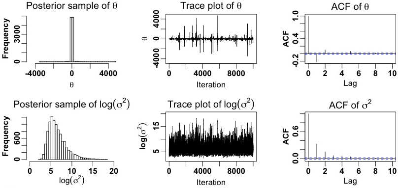
Figure 1: The result of sampling an improper posterior distribution in Equation (4). The histogram, trace plot, and auto-correlation function of 10,000 posterior samples of $\theta$ are on the top panels and those of $\log(\sigma^{2})$ on the bottom panels. The Markov chain appears to converge to a certain probability distribution, although the target posterior distribution in Equation (4) is not a probability distribution.

In Figure 1, we display the histogram, trace plot, and auto-correlation function of 10,000 posterior samples of $\theta$ on the top and those of $\log(\sigma^{2})$ on the bottom. The posterior sample of $\theta$ concentrates on zero and that of $\log(\sigma^{2})$ also forms a unimodal histogram. The trace plots show that the Markov chain explores the parameter space rapidly and the auto-correlation functions decrease quickly. The effective sample size of $\theta$ is black8,140 and that of $\log(\sigma^{2})$ is black1,847. Clearly, the Markov chain appears to converge to a certain probability distribution, and thus it makes sense to make a probabilistic inference using this posterior sample. However, if the initial value of $\sigma^{2}$ were close to zero at which the posterior kernel function puts infinite mass, the Markov chain would stay at $\sigma^{2}=0$ permanently without producing such a seemingly reasonable posterior sample. blackSee Hobert and Casella, (1996) for more theoretical details.

Such an inappropriate probabilistic inference based on a non-blackexisting probability distribution can actually happen in reality unless posterior propriety is proven in advance. The article of Pihajoki, (2017) published in MNRAS uses a similar but more complicated Gaussian hierarchical model that can be built upon a marginalized model of Equation (2), that is,

$$y_{j}\mid\theta,\sigma^{2}\sim\textrm{N}(\theta,V_{j}+\sigma^{2}).$$ (6)

blackA model of Pihajoki, (2017) replaces $\theta$ in Equation (6) with $\alpha+\beta x_{j}$, where $\alpha$ and $\beta$ are unknown regression coefficients and $x_{j}$ is some known covariate information with its known measurement variance $V_{x_{j}}$. Also, blackthe model replaces $V_{j}$ in Equation (6) with $\beta^{2}V_{x_{j}}+V_{j}-2\beta\rho(V_{x_{j}}V_{j})^{0.5}$, multiplies $\sigma^{2}$ in Equation (6) by black$1+\beta^{2}$, and adopts an improper blackjoint prior $\textcolor{black}{d\alpha}d\sigma/\sigma$; see Equations (33)–(37) of Pihajoki, (2017). blackThis improper joint prior is equivalent to the problematic choice in Equation (3). The resulting posterior is not a probability distribution. This is because when $\beta=0$, the model of Pihajoki, (2017) becomes exactly the same as the one in Equation (6) that is improper with $\textcolor{black}{d\alpha}d\sigma/\sigma$. Therefore, the integral of the posterior kernel function of Pihajoki, (2017) is not finite.
blackThe article of Pihajoki, (2017) does not check posterior propriety before using an MCMC method. Thus, without recognizing posterior impropriety, the article makes a probabilistic inference using the seemingly reasonable posterior sample drawn from a non-existent posterior distribution. An MCMC method for this model may not show blackany evidence of posterior impropriety unless a Markov chain starts with the initial value of $\sigma^{2}$ close to zero. In practice, blackhowever, the inference blackin Pihajoki, (2017) may be similar to blackthat based on a proper posterior equipped with weakly informative proper priors. This is because it is likely that the blackMarkov chain of Pihajoki, (2017) resides in a safe (high-likelihood) region without exploring the entire parameter space.
blackOne may think that we are exaggerating a problem with a pathological example where a tiny corner of the parameter space becomes a problem. We emphasize again that our concern is whether researchers are clearly aware that their Bayesian inferences are based on probability distributions. We have used such a tiny parameter space, e.g, $\sigma^{2}\in[0,\epsilon)$ and $\beta=0$, to raise a question about this concern, not to criticize Pihajoki, (2017)’s omission in exploring this pathological region. Exploring the entire parameter space, however, is a useful practice to check a Markov chain’s convergence. Inconsistent results from multiple Markov chains, whose initial values are spread across the parameter space, indicate the lack of convergence, e.g., due to multimodality or possibly posterior impropriety. A popular convergence diagnostic statistic of Gelman and Rubin (1992) is based on this idea. Initiating multiple Markov chains at least one of which begins near $\sigma^{2}=0$ might have indicated posterior impropriety in the case of Pihajoki, (2017).
blackAn astronomer’s intuition or prior knowledge may indicate which parameter space is scientifically meaningful to search a priori. This is invaluable information, but should be used carefully because one may have an incentive to initiate a Markov chain only in such a specific part of the parameter space. This chain might have stayed in that part, inevitably producing a result that is consistent with the astronomer’s intuition. But, it is not desirable to report this result as if the entire parameter space were explored (even though a physically inspired model may have more power to constrain the region of interest than a non-physically inspired ones). Without being fully informed of such a limited search, readers may assume that evidence for multiple modes or posterior impropriety has not been found in the entire parameter space. Therefore, it is desirable to run multiple Markov chains with widely spread initial values across the parameter space or to use more tightly bounded priors to clarify which part is actually explored.

3 Posterior propriety in the astronomical literature

We investigated the literature published online in ApJ and MNRAS between Jan 1, 2017 and Oct 15, 2017. blackOn the webpages of IOPscience and MNRAS, we found 75 articles whose titles or abstracts contain a word ‘Bayesian’black; see Appendix C for details of the selection. None of the 75 articles mention posterior propriety, and thus we blackchecked further by classifying them into three categories; (a) priors are jointly proper; (b) priors are jointly improper; and (c) priors are not clearly specified. The last category includes cases where uniform (or flat) prior distributions are used without clearly specified ranges. Table 1 summarizes the classification; blackalso see Appendix C for details. More than half of the articles use jointly proper priors. blackHowever, there are black23 articles in categories (b) and (c) that need proofs for posterior propriety to assure that their scientific arguments are actually based on blackproper posterior distributions.

The issue of the 20 articles in category (c) is not only posterior propriety but also reproducibility because blacktheir results cannot be reproduced without information about their priors. blackFor instance, there are infinitely many uniform prior distributions according to their ranges, and thus a flat uniform prior is not a clear description. Proving posterior propriety can contribute to reproducible science as a by-product because its first step is to blackspecify a Bayesian model blackclearly, i.e., a likelihood function of unknown parameters and their prior distributions.

blackWithout hurting readability, one may be able to specify both likelihood function and priors in an appendix, mentioning only the resulting posterior propriety in the main text. This practice will greatly improve statistical clarity and reproducibility in the astronomical literature.

Table 1: Classification of 75 articles published online in $ApJ$ and $MNRAS$ between Jan 1, 2017 and Oct 15, 2017 according to their prior distributions.

	$ApJ$	$MNRAS$
(a) Jointly proper priors	18	black34
(b) Jointly improper priors	1	black2
(c) Unclear priors	11	9
Total	30	45

4 Discussion

4.1 blackProving posterior propriety

Improper prior distributions are widely used because they are blackmathematically convenient and blackare considered non-informative. blackA uniform($-\infty,\infty$) prior on a location parameter, e.g., $p_{1}(\theta)$ in Equation (3), blackis a Jeffreys’ prior. It also has an advantage to make the data (likelihood function) speak more about the parameter when prior knowledge is limitedblack, and results in a proper posterior distribution in many cases.

However, there is a cost to be paid for using improper priors, which is often neglected: Proving posterior propriety. blackAdopting an improper prior for even one parameter requires proving that the integral of a posterior kernel function over the entire parameter space is finite. It is challenging to develop a universal rule-of-thumb about when improper priors are likely to cause improper posterior and when they are not. This is because posterior propriety cannot be assured before it is actually proven on a case by case basis. The problematic choice $d\sigma^{2}/\sigma^{2}$ in Section 2, for example, does not cause posterior impropriety for a different Gaussian model such as $y_{j}\mid\mu,\sigma^{2}\sim\textrm{N}(\mu,\sigma^{2})$. With $p(\mu,\sigma^{2})\propto 1/\sigma^{2}$, the resulting posterior is proper if $n\geq 2$; see Appendix D for a proof.
There are several ways to prove blackposterior propriety. The most rigorous one is to analytically show that the integral of the target posterior kernel function blackover the entire parameter space is finite. However, if the dimensions are large and the model is complicated, blackwhich is usually the case in the astronomical literature, it is challenging to prove posterior propriety analytically.
blackWe can also apply existing theorems about posterior propriety only if a model considered in a theorem is the same as a blackcandidate model to be used. For example, suppose a blackcandidate model has two more parameters than a model whose posterior propriety is proven in a theorem. Posterior propriety of blackthe candidate model holds if a marginalized blackcandidate model (with the two additional parameters integrated out from blackthe candidate model) is the same as blackthe model considered in the theorem. This is because an unexpected term that is a function of unknown parameters may arise during the integration, which can make seemingly similar models completely different.

Jointly proper priors guarantee posterior propriety based on standard probability theory. blackThus, when researchers want to adopt physically motivated improper priors whose posterior propriety is challenging to be proven, it is a useful practice to adopt proper priors that can mimic the behavior of the improper ones. The resulting posterior inference with mimicking proper priors will be almost identical to the one with improper priors. For a location parameter whose support is a real line, e.g., $\theta$ in Equation (3), a diffuse Gaussian or diffuse Student’s $t$ prior blackwith an arbitrarily large scale can approximate an improper flat prior. The arbitrarily large scale of such a diffuse prior is a computational trick to approximate the improper flat prior although the scale itself may not make sense in practice. As for a parameter blackdefined on a positive real line, e.g., $\sigma^{2}$ in Equation (3), a log-Normal, half Normal, and half Student’s $t$ with relatively large variance are known to be vague choices (Gelman,, 2006) blackthat can approximate an improper flat prior $d\sigma^{2}$. blackAlso, a uniform shrinkage prior, $d\sigma^{2}/(c+\sigma^{2})^{2}$, where $c$ is set to an arbitrarily large constant, can approximate $d\sigma^{2}$ with good frequentist coverage properties (Tak,, 2017).

4.2 blackScientifically motivated proper priors for posterior propriety

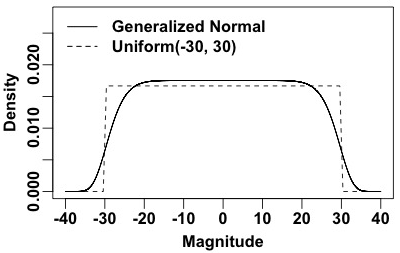
Figure 2: blackPrior distributions of magnitude. The density of the generalized Gaussian distribution with $\mu=0$, $\sigma=30$, and $s=10$ is denoted by a solid curve and that of the uniform($-30,30$) distribution is represented by a dashed curve. As $s$ increases, the two densities become close in shape. Unlike the uniform distribution whose hard bounds completely exclude a certain range of magnitude, the generalized Gaussian distribution sets up soft bounds.

blackAdopting scientifically motivated priors is one advantage of using Bayesian machinery because it provides a natural way to incorporate scientific knowledge into inference via priors. Proper priors are ideal for this purpose. Tak et al., (2017), for example, use a uniform($-30,30$) prior for the unknown mean magnitude of a damped random walk process, considering a practical magnitude range from that of the Sun to that of the faintest object identifiable by the Hubble Space Telescope. This prior can be considered weakly informative because the range of the uniform prior is wide enough not to affect the resulting posterior inference. (A bounded uniform prior is not non-informative because its hard bounds completely exclude a certain range of parameter values.) If the range of a uniform prior is narrow and thus it significantly influences the posterior inference, such an informative choice may need further justification.

blackIf one is uncomfortable about completely excluding a certain parameter space, a generalized Gaussian distribution (Nadarajah,, 2005, 2006), also called a power exponential distribution, can be used to set up soft bounds. These soft bounds allow values outside the bounds with small but non-zero probability. Its kernel function of $x$ is proportional to $\exp(-|(x-\mu)/\sigma|^{s})$, where $\mu$ is the location parameter, $\sigma$ is the scale parameter, and $s$ is the shape parameter. The distribution approaches the uniform($\mu-\sigma,\mu+\sigma$) distribution, i.e., the tails of its density decrease more sharply, as $s$ goes to infinity. Figure 2 displays its density function for $\mu=0$, $\sigma=30$, and arbitrarily chosen shape parameter $s=10$ with the density of uniform($-30,30$) superimposed. A generalized Student’s $t$ distribution (McDonald and Newey,, 1988) can be an alternative if one prefers geometrically decreasing tails so that the data (likelihood) can dominate these bounds more easily (i.e., less informative).

For an unknown parameter whose support is the positive real line, an inverse-Gamma prior can be used as a scientifically motivated prior because it enables us to set up a soft lower bound of a parameter using scientific knowledge or past studies. The kernel function of $x$ that follows an inverse-Gamma($a,b$) distribution is $x^{-a-1}\exp(-b/x)$. Its mode, $b/(a+1)$, plays a role of the soft lower bound, and a small shape parameter $a$ is desirable for a weakly informative prior. When $x$ goes to infinity, the right tail of this kernel function decreases as a power law, while the left tail exponentially decreases as $x$ approaches zero. Thus $x$ is less likely to take on values much smaller than the mode (soft lower bound) a priori. blackSee Figure 3 for a few density curves of inverse-Gamma($a,b$) prior according to different values of $a$ and $b$. Modeling quasar variability, for example, Tak et al., (2017) adopt an inverse-Gamma(1, $b$) prior for the unknown timescale (in days) of a damped random walk process. The scale parameter $b$ is set to one day so that its soft lower bound, 0.5 day, is much smaller than any timescale estimates of 9,275 quasars in a past study (MacLeod et al.,, 2010) a priori.

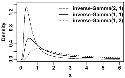
Figure 3: blackThree inverse-Gamma($a,b$) densities according to different shape and scale parameters, $a$ and $b$. We suggest using an inverse-Gamma($a,b$) prior as a way to set up a soft lower bound of a random variable $x$ a priori. The right tail geometrically decreases with power $a+1$ and the left tail exponentially decreases, which indicates that $x$ is less likely to take on values much smaller than the mode (soft lower bound), $b/(a+1)$, a priori. A small value of the shape parameter is desirable for a weakly informative prior. Fixing the shape parameter first ($a\ll n$), we can adjust the scale parameter to set a scientifically motivated soft lower bound.

For a second-level variance component in a Gaussian hierarchical model such as $\sigma^{2}$ in Equation (2), Gelman, (2006) does not recommend an inverse-Gamma($a,b$) prior with arbitrarily small values blackfor both $a$ and $b$ as a non-informative choice. This makes sense because an inverse-Gamma prior always sets up a soft lower bound a priori. When the likelihood puts significant weight at zero but with relatively small data size, it is difficult for the likelihood to dominate the soft lower bound blackthat is located near zero. In this case, the resulting posterior inference becomes sensitive to the location of the soft lower bound. Thus when the data size is small, it is important to construct the soft lower bound carefully, considering scientific knowledge or past studies.

Table 2: blackA few proper priors that can be set up easily to reflect scientific knowledge and past studies in a weakly informative way.

blackDistribution	blackSupport	blackKernel function	blackNote
blackuniform($a,b$)	black$\mathbb{R}$	black$1/(b-a)$	blackIts hard bounds $(a,b)$, where $a<b~{}(\in\mathbb{R})$, can reflect past studies.
blackgeneralized Gaussian	black$\mathbb{R}$	black$\exp(-|(x-\mu)/\sigma|^{s})$	black$\mu~{}(\in\mathbb{R})$ is the location parameter, $\sigma~{}(\in\mathbb{R}^{+})$ is the scale parameter, and
			black$s~{}(\in\mathbb{R}^{+})$ is the shape parameter. As $s\to\infty$, this distribution becomes
			blackuniform($\mu-\sigma,\mu+\sigma$), and thus $(\mu-\sigma,\mu+\sigma)$ can be considered as
			blacksoft bounds set to represent scientific knowledge. The choice of $s$ may be
			blackarbitrary. A generalized $t$ distribution can be an alternative whose tails
			blackdecreases geometrically.
blackinverse-Gamma($a,b$)	black$\mathbb{R}^{+}$	black$x^{-a-1}\exp(-b/x)$	black$a~{}(\in\mathbb{R}^{+})$ is the shape parameter and is treated as the amount of prior
			blackinformation. It is desirable to be small for a weakly informative prior
			black($a\ll n$). Given $a$, the scale parameter $b~{}(\in\mathbb{R}^{+})$ is set to form a soft lower
			blackbound $b/(a+1)$ that represent past studies.
blackmultiply-broken	black$\mathbb{R}^{+}$	black$x^{-\alpha_{1}}I_{(0<x\leq b_{1})}\textcolor{black}{+}$	blackSmall values of powers, $\alpha_{1},\ldots,\alpha_{k}$, are desirable for a weakly informative
blackpower-law		$\textcolor{black}{\beta_{2}}x^{-\alpha_{2}}I_{(b_{1}<x\leq b_{2})}\textcolor{black}{+}$	prior. blackWhen $k=1$, $\alpha_{1}\in[0,1)$ and $b_{0}=0$. If $k=2$, $\alpha_{1}\in[0,1)$ and $\alpha_{2}>1$.
		$\cdots\textcolor{black}{+}$	blackFor $k\geq 3$, $\alpha_{1}\in[0,1)$, $\alpha_{j}\geq 0~{}\textrm{for}~{}j=2,3,\ldots,k-1$, and $\alpha_{k}>1$. Segment-
		$\textcolor{black}{\beta_{k}}x^{-\alpha_{k}}I_{(b_{k-1}<x)}$	blackwise uniform priors are feasible if $\alpha_{i}=0$ ($i\neq k$). blackIf $\beta_{i}=b_{i-1}^{\alpha_{i}-\alpha_{i-1}}$ for $i\geq 2$,
			blackthis power law becomes a continuous function. All powers blackand coefficients,
			black$\alpha_{i}$, $b_{i}$, and $\beta_{i}$, can reflect scientific knowledge.

blackA multiply-broken power-law density, proposed by Professor Eric B. Ford during a personal communication, can be another easy-to-construct scientifically inspired prior for parameters defined on a positive real line. For example, a doubly-broken power-law density is defined as $p(x)\propto x^{-\alpha_{1}}$ for $0<x\leq b_{1}$, $\textcolor{black}{p(x)=\beta_{2}x^{-\alpha_{2}}}$ for $b_{1}<x\leq b_{2}$, and $\textcolor{black}{p(x)=\beta_{3}x^{-\alpha_{3}}}$ for $b_{2}<x$. blackIf $\beta_{i}=b_{i-1}^{\alpha_{i}-\alpha_{i-1}}$ for $i=2,3$, it becomes a smoothly broken power-law (e.g., Anchordoqui et al.,, 2014). Small blackvalues of powers, $\alpha_{1}\textcolor{black}{(<1)}$, $\alpha_{2}$, and $\alpha_{3}$ $(>\!1)$, are desirable for weakly informative priors, and zero powers for $\alpha_{1}$ and $\alpha_{2}$ enable segment-wise uniform priors. All these parameters including the cut-offs $b_{1}$ and $b_{2}$ ($0<b_{1}<b_{2}$) need to reflect astronomical knowledge or past studies.

blackWe summarize all these proper priors in Table 2.

4.3 blackRe-analysis of the example in Section 2 with jointly proper priors

Let us revisit the example in Section 2 to see an impact of adopting jointly proper priors. Instead of the improper choiceblacks in Equation (3), we set a diffuse Gaussian prior for $\theta$ and a weakly informative inverse-Gamma prior for $\sigma^{2}$ independently:

$$\theta\sim\textrm{N}(0,~{}10^{5})~{}~{}\textrm{and}~{}~{}\sigma^{2}\sim\textrm{inverse-Gamma}(\textcolor{black}{10^{-2},1}).$$ (7)

blackWe first set the shape parameter of the inverse-Gamma($a,b$) prior to $10^{-2}$ that is much smaller than the data size ($a\ll n$). Next we set $b=1$ to construct a soft lower bound, 0.99, assuming that it reflects scientific knowledge a priori. We denote the joint prior distribution in Equation (7) by $p^{\ast}(\theta,\sigma^{2})$. The resulting full posterior kernel function is

$$q^{\ast}(\boldsymbol{\mu},\theta,\sigma^{2}\mid\boldsymbol{y})=p^{\ast}(\theta,\sigma^{2})\prod_{j=1}^{n}\left[f(y_{j}\mid\mu_{j})~{}p(\mu_{j}\mid\theta,\sigma^{2})\right],$$ (8)

where density functions $f$ and $p$ are defined in Equation (2). The corresponding Gibbs sampler updates each coordinate of $\boldsymbol{\mu}$ by its conditional posterior specified in Equation (LABEL:conditionals) but updates $\theta$ and $\sigma^{2}$ by

$$\begin{aligned} \theta\mid\boldsymbol{\mu},\sigma^{2},\boldsymbol{y}&\sim\textrm{N}\left(~{}\frac{(n/\sigma^{2})\bar{\mu}}{n/\sigma^{2}+1/10^{5}},~{}\frac{1}{n/\sigma^{2}+1/10^{5}}~{}\right),\\ \sigma^{2}\mid\boldsymbol{\mu},\theta,\boldsymbol{y}&\\ \sim\textrm{inverse}&\textrm{-Gamma}\left(~{}\frac{n}{2}+\frac{1}{10^{2}},~{}\frac{\sum_{j=1}^{n}(\mu_{j}-\theta)^{2}}{n}+1~{}\right).\end{aligned}$$ (9)

blackThe conditional distribution of $\theta$ in Equation (9) is similar to that in Equation (LABEL:conditionals), considering that $10^{-5}$ is close to zero. The other simulation configuration is the same.

Figure 4 exhibits the sampling result. The ranges of the horizontal and vertical axes in each panel are the same as those of Figure 1 for a comparison. Because of the jointly proper priors in Equation (7), we know that the resulting posterior kernel function $q^{\ast}$ in Equation (8) is proper and thus the posterior sample displayed in Figure 4 represents the target posterior distribution. Although not shown here, the MCMC method produces nearly the same sampling result regardless of the initial value of $\sigma^{2}$black, meaning that the Markov chain converges no matter where it starts. The histogram of $\theta$ in Figure 4 has much shorter tails than that in Figure 1, although the histogram of $\log(\sigma^{2})$ in Figure 4 is similar to that in Figure 1. The soft lower bound of $\log(\sigma^{2})$, i.e., black$\log(0.99)=-0.01$, is not close to the high density region. This indicates that blackthe soft lower bound does not affect the blackresulting posterior inference even though there are just two data points; the degrees of freedom blackparameter of an equivalent inverse-$\chi^{2}$ prior blackis 0.02. blackA sensitivity analysis, though not shown here, indicates that the results are robust as long as the scale parameter $b$ of the inverse-Gamma($10^{-2},b$) prior puts the soft lower bound on the left-hand side of the high-density region. The effective sample size improves greatly; it is black9,823 for $\theta$ and black2,668 for $\log(\sigma^{2})$. Consequently, the inference on $\theta$ becomes quite different from that in Section 2, empirically blackshowing that checking posterior propriety before using MCMC methods can make a significant difference.

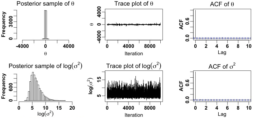
Figure 4: The result of sampling the proper posterior kernel function in Equation (8) that is based on weakly informative and vague proper priors in Equation (7). The histogram, trace plot, and auto-correlation function of 10,000 posterior samples of $\theta$ are on the top panels and those of $\log(\sigma^{2})$ on the bottom panels. The ranges of vertical and horizontal axes are the same as those in Figure 1. Since priors in Equation (7) are jointly proper, we know that the resulting posterior $q^{\ast}$ in Equation (8) is proper and thus the posterior sample is from $q^{\ast}$. Also, the sampling result hardly varies even if the initial value of $\sigma^{2}$ is close to zero. The ensuing Bayesian inference on $\theta$ is quite different from that in Section 2 with much shorter tails.

4.4 blackConcluding remarks

It is well understood that any probabilistic blacktool such as Bayesian blackinterface should be based on a probability distribution. Jointly proper priors lead to a proper posterior distribution and can be either vague or scientifically motivated. However, improper priors are sometimes used to represent the lack of prior knowledge. Such improper priors combined with a likelihood function can result in an improper posterior distribution that is not blacka probability measure. Therefore, when improper priors are adopted, posterior propriety must be carefully proven before using any MCMC methodsblack, which can also improve statistical clarity and reproducibility. We hope that posterior propriety draws more attention when improper priors are used in the astronomical literature.
blackFor a more complete Bayesian analysis, posterior propriety is not the only thing to be checked in practice. We list some procedures or practices essential for a good Bayesian analysis as the referee recommends. Above all, we re-emphasize the importance of clarifying a Bayesian model, i.e., clearly specifying both likelihood function and priors, which is the beginning of the Bayesian analysis that precedes even checking posterior propriety. During the analysis, it is important to explore the entire (pre-specified) parameter space by implementing multiple Markov chains whose initial values are spread across the parameter space; it is desirable to specify the initial values of the chains. After the analysis, a good Bayesian analysis comes with various diagnostic procedures. An MCMC convergence check is necessary in both visual and numerical ways, e.g., trace plots, auto-correlation functions, effective sample sizes, and Gelman-Rubin diagnostic statistics (Gelman and Rubin,, 1992). As for model checking (Section 6, Gelman et al.,, 2013), a posterior predictive check is a valuable tool to assess a model’s consistency with the observed data, i.e., whether the model can explain the data generation process well. A prior predictive check (if priors are proper) is also useful for model checking, which generates a data set using a model with known parameter values and checks whether a fitted model can recover the generative parameter values. In addition, a sensitivity check is important to understand the influence of prior assumptions on the resulting posterior inference. We hope good Bayesian practice becomes more popular in the astronomical literature for more reliable Bayesian analysis.

Appendix A The Bayes Theorem in Detail

It is well known that a Bayesian statistical model consists of (i) a sampling distribution, $f(\boldsymbol{y}\mid\boldsymbol{\theta})$, denoting the conditional probability density of the data $y$ given unknown parameters $\boldsymbol{\theta}$; and (ii) a prior distribution, $p(\boldsymbol{\theta})$, denoting an unconditional probability density of $\boldsymbol{\theta}$. The resulting joint density of $\boldsymbol{y}$ and $\boldsymbol{\theta}$ is $f(\boldsymbol{y}\mid\boldsymbol{\theta})p(\boldsymbol{\theta})$ based on standard probability theory. We can also express this joint density as a product of the unconditional density of the data $h(\boldsymbol{y})\equiv\int f(\boldsymbol{y}\mid\boldsymbol{\theta})p(\boldsymbol{\theta})d\boldsymbol{\theta}$ and the so-called posterior density of $\boldsymbol{\theta}$ given $\boldsymbol{y}$, i.e.,

$$\pi(\boldsymbol{\theta}\mid\boldsymbol{y})=\frac{f(\boldsymbol{y}\mid\boldsymbol{\theta})p(\boldsymbol{\theta})}{\int f(\boldsymbol{y}\mid\boldsymbol{\theta})p(\boldsymbol{\theta})d\boldsymbol{\theta}}.$$ (10)

All density functions are formally defined with respect to Lebesgue measure (or counting measure). However, in many scientific applications, we may relax the need for the use of a probability measure for the prior distribution by using a kernel function $k(\boldsymbol{\theta})=c_{0}p(\boldsymbol{\theta})$ for some constant $c_{0}>0$ and also write the likelihood function $L(\boldsymbol{\theta};\boldsymbol{y})=c(\boldsymbol{y})f(\boldsymbol{y}\mid\boldsymbol{\theta})$ for some function $c(\boldsymbol{y})>0$. Then, as illustrated in Ghosh, (2010), we can reexpress Equation (10) as

$$\pi(\boldsymbol{\theta}\mid\boldsymbol{y})=\frac{f(\boldsymbol{y}\mid\boldsymbol{\theta})p(\boldsymbol{\theta})}{\int f(\boldsymbol{y}\mid\boldsymbol{\theta})p(\boldsymbol{\theta})d\boldsymbol{\theta}}=\frac{L(\boldsymbol{\theta};\boldsymbol{y})k(\boldsymbol{\theta})}{\int L(\boldsymbol{\theta};\boldsymbol{y})k(\boldsymbol{\theta})d\boldsymbol{\theta}}.$$ (11)

As illustrated in Section 1, even if $\int k(\boldsymbol{\theta})d\boldsymbol{\theta}=\infty$, making the prior distribution improper, the posterior density as given in Equation (11) is still a valid probability density as long as the denominator $\int L(\boldsymbol{\theta};\boldsymbol{y})k(\boldsymbol{\theta})d\boldsymbol{\theta}<\infty$ is finitely integrable. However, an improper prior necessarily leads to improper marginal distribution of the data $\boldsymbol{y}$ (and vice versa), i.e., $\int k(\boldsymbol{\theta})d\boldsymbol{\theta}=\infty$ is equivalent to $\int h(\boldsymbol{y})d\boldsymbol{y}=\infty$. This is because

$$\int h(\boldsymbol{y})d\boldsymbol{y} =\int\int f(\boldsymbol{y}\mid\boldsymbol{\theta})p(\boldsymbol{\theta})d\boldsymbol{\theta}~{}\!dy$$

$$=\int\int f(\boldsymbol{y}\mid\boldsymbol{\theta})p(\boldsymbol{\theta})d\boldsymbol{y}~{}\!d\boldsymbol{\theta}=\int p(\boldsymbol{\theta})d\boldsymbol{\theta},$$

where the second equality holds from Fubini’s theorem. This aspect is not a concern if $\pi(\boldsymbol{\theta}\mid\boldsymbol{y})$ is a proper probability density. It is well known that, in order to make an inference about $\boldsymbol{\theta}$ (or its function) conditional on the observed data, it is often sufficient to draw samples from a posterior kernel given by $L(\boldsymbol{\theta};\boldsymbol{y})k(\boldsymbol{\theta})$, i.e., the numerator in Equation (11) without the need to evaluate the denominator. Unfortunately, Gibbs-type MCMC methods can generate a sample from the posterior kernel which need not correspond to a proper posterior distribution; see Hobert and Casella, (1996) for various examples. When a proper prior density $p(\boldsymbol{\theta})$ is used, this is not an issue as a posterior distribution is necessarily proper by standard probability theory. However, when an improper prior kernel is used, then the only option is to verify analytically that integral in the denominator of Equation (11) is finite.

Appendix B Proof of Posterior Impropriety in Section 2

The full posterior kernel function $q(\boldsymbol{\mu},\theta,\sigma^{2}\mid\boldsymbol{y})$ in Equation (4) is improper because the marginal posterior kernel function $q_{1}(\sigma^{2}\mid\boldsymbol{y})$ with $\boldsymbol{\mu}$ and $\theta$ integrated out from $q(\boldsymbol{\mu},\theta,\sigma^{2}\mid\boldsymbol{y})$ is improper. We derive the marginal posterior kernel function of $\theta$ and $\sigma^{2}$ by integrating out $\boldsymbol{\mu}$ from $q(\boldsymbol{\mu},\theta,\sigma^{2}\mid\boldsymbol{y})$:

$$\begin{aligned} q_{2}(\theta,&~{}\sigma^{2}\mid\boldsymbol{y})=\int_{\mathbb{R}^{n}}q(\boldsymbol{\mu},\theta,\sigma^{2}\mid\boldsymbol{y})~{}d\boldsymbol{\mu}\\ &=p_{1}(\theta,\sigma^{2})\prod_{j=1}^{n}f_{1}(y_{j}\mid\theta,V_{j}+\sigma^{2})\\ &=\frac{1}{\sigma^{2}}\exp\left(-\sum_{j=1}^{n}\frac{(y_{j}-\theta)^{2}}{2(V_{j}+\sigma^{2})}\right)\prod_{j=1}^{n}(V_{j}+\sigma^{2})^{-0.5}\\ &=\frac{1}{\sigma^{2}}\exp\left(-\sum_{j=1}^{n}\frac{(y_{j}-\hat{y})^{2}}{2(V_{j}+\sigma^{2})}-\frac{(\theta-\hat{y})^{2}}{2V^{\ast}}\right)\prod_{j=1}^{n}(V_{j}+\sigma^{2})^{-0.5},\end{aligned}$$ (12)

where density functions $p_{1}$ and $f_{1}$ are defined in Equations (3) and (6), respectively,

$$\hat{y}\equiv\frac{\sum_{j=1}^{n}y_{j}/(V_{j}+\sigma^{2})}{\sum_{j=1}^{n}1/(V_{j}+\sigma^{2})}~{}~{}\textrm{and}~{}~{}V^{\ast}\equiv\frac{1}{\sum_{j=1}^{n}1/(V_{j}+\sigma^{2})}.$$

Next we marginalize out $\theta$ from Equation (12) as follows:

$$q_{1}(\sigma^{2}\mid\boldsymbol{y}) =\int_{\mathbb{R}}q_{2}(\theta,\sigma^{2}\mid\boldsymbol{y})~{}d\theta$$

$$=\frac{(V^{\ast})^{0.5}}{\sigma^{2}}\exp\left(-\sum_{j=1}^{n}\frac{(y_{j}-\hat{y})^{2}}{2(V_{j}+\sigma^{2})}\right)\prod_{j=1}^{n}(V_{j}+\sigma^{2})^{-0.5}.$$ (13)

This marginal posterior kernel function of $\sigma^{2}$ approaches infinity as $\sigma^{2}$ goes to zero due to the prior on $\sigma^{2}$, i.e., $d\sigma^{2}/\sigma^{2}$. Therefore, $\int_{\mathbb{R}^{+}}q_{1}(\sigma^{2}\mid\boldsymbol{y})~{}d\sigma^{2}=\infty$.

Appendix C Classification of 75 articles in Section 3

blackOn the webpage of IOPscience, we found 33 ApJ articles whose titles or abstracts contain a word ‘Bayesian’. We excluded three of them because one is an erratum (Eadie et al., 2017b, ) and the other two use just Bayesian methods previously developed by other researchers (Abeysekara et al.,, 2017; Murphy et al.,, 2017). We also obtained a list of 51 articles from the webpage of MNRAS that have the word ‘Bayesian’ in their abstracts. We did not consider six of them because one mentions a Bayesian analysis as a potential application (Watkinson et al.,, 2017), another uses a Bayesian information criterion for a model selection (Wilkinson et al.,, 2017), and the other four simply utilize Bayesian methods developed in other articles (Pinamonti et al.,, 2017; Green et al.,, 2017; Sampedro et al.,, 2017; Basak et al.,, 2017).

Among the 30 articles published online in ApJ, 18 articles adopt jointly proper priors, and we classify these into category (a); Fogarty et al., (2017); Montes-Solís and Arregui, (2017); Zevin et al., (2017); Leung et al., (2017); Farnes et al., (2017); Benson et al., (2017); Sathyanarayana Rao et al., (2017); Sliwa et al., (2017); Park et al., (2017); Khrykin et al., (2017); Budavári et al., (2017); Wang et al., (2017); Scherrer and McKenzie, (2017); Tabatabaei et al., (2017); Lund et al., (2017); Eadie et al., 2017a ; Martínez-García et al., (2017); Küpper et al., (2017).

Knežević et al., (2017) set an unbounded flat prior on the logarithm of the total flux without proving posterior propriety, and thus we classify this article into category (b).

We cannot check posterior propriety of 11 articles published online in ApJ because they do not specify priors clearly, i.e., their Bayesian models are not uniquely determined. We designate them as category (c) which contains cases where uniform (or flat) priors are used without clear ranges. Here we list them; Kern et al., (2017) use flat priors over the astrophysical parameters; Bitsakis et al., (2017) say nothing about priors; Raithel et al., (2017) do not specify a joint prior on five pressures; Oyarzún et al., (2017) utilize flat priors on all parameters; Tanaka et al., (2017) make use of uniform priors on $m_{\textrm{TRGB}}$ and $a$; Mandel et al., (2017) adopt a flat prior on $\mu_{s}$ whose range is unclear; Daylan et al., (2017) adopt uniform priors on many parameters; Warren et al., (2017) utilize an uninformative prior on $\beta$; Solá et al., (2017) make use of an uninformative prior on $h$; Eilers et al., (2017) do not specify priors on $\gamma$, $\sigma_{C}$, and $\sigma_{ij}$; and Jones et al., (2017) use flat priors on SN Ia distances.

Next, we classify 45 articles published online in MNRAS into three categories. Category (a) contains black34 articles whose priors are jointly proper; Ashton et al., (2017); Bainbridge and Webb, (2017); Ata et al., (2017); Wagner-Kaiser et al., (2017); Cibirka et al., (2017); Patel et al., (2017); Si et al., (2017); Dwelly et al., (2017); Maund, (2017); Davis et al., (2017); Hahn et al., (2017); Burgess, (2017); Silburt and Rein, (2017); MacDonald and Madhusudhan, (2017); Abdurro’uf and Akiyama, (2017); Kafle et al., (2017); Aigrain et al., (2017); Henderson et al., (2017); Kimura et al., (2017); Schellenberger and Reiprich, (2017); Mejía-Narváez et al., (2017); Köhlinger et al., (2017); Dam et al., (2017); Garnett et al., (2017); Andrews et al., (2017); Kovalenko et al., (2017); McEwen et al., (2017); Oh et al., (2017); Duncan et al., (2017); Galvin et al., (2017); Salvato et al., (2017); Yu and Liu, (2017); Greig and Mesinger, (2017); blackand Sereno and Ettori, (2017).

blackTwo articles published online in MNRAS employ improper priors without proving posterior propriety; Kos, (2017) sets an improper prior on $l_{\textrm{se}}$ without an upper limit; and we proved posterior impropriety of Pihajoki, (2017) resulting from the improper prior on $\sigma^{2}$.

We cannot judge posterior propriety of 9 articles published in MNRAS because their priors are not clearly specified; Rodrigues et al., (2017) adopt flat priors on metallicity and age; Vallisneri and van Haasteren, (2017) do not specify priors on $\sigma_{\textrm{out}}$ and $c$; Binney and Wong, (2017) use uniform priors for the logarithm of scale parameters; Ashworth et al., (2017) use flat priors on $\alpha_{3}$ and $A_{V}$; Jeffreson et al., (2017) utilize uniform priors on eight parameters (three are on the logarithmic scale); Molino et al., (2017) adopt flat priors on galaxy type and redshift; Accurso et al., (2017) do not specify priors on $\alpha$ and $\beta_{j}$; Günther et al., (2017) adopt uniform priors on all parameters; and Igoshev and Popov, (2017) do not clarify a joint prior on $\vec{v}_{o}$.

Appendix D Proof of Posterior Propriety in Section 4

blackThe target posterior kernel function of $\mu$ and $\sigma^{2}$ is as follows:

$$\pi(\mu,\sigma^{2}\mid\boldsymbol{y})\propto(\sigma^{2})^{n/2-1}\exp\left[-\frac{\sum_{i=1}^{n}(y_{i}-\mu)^{2}}{2\sigma^{2}}\right].$$ (14)

The marginal posterior kernel function of $\sigma^{2}$ with $\mu$ integrated out from Equation (14) is

$$\pi(\sigma^{2}\mid\boldsymbol{y})\propto(\sigma^{2})^{-(n-1)/2-1}\exp\left[-\frac{\sum_{i=1}^{n}(y_{i}-\bar{y})^{2}}{2\sigma^{2}}\right].$$ (15)

The integral of $\pi(\sigma^{2}\mid\boldsymbol{y})$ in Equation (15) is finite if $n$ is greater than 1 because the marginal posterior distribution of $\sigma^{2}$ is inverse-Gamma($(n-1)/2,~{}\sum_{i=1}^{n}(y_{i}-\bar{y})^{2}/2$), considering the functional form of $\pi(\sigma^{2}\mid\boldsymbol{y})$ in Equation (15).

References

- Abdurro’uf and Akiyama, (2017) Abdurro’uf and Akiyama, M. (2017). Understanding the Scatter in the Spatially Resolved Star Formation Main Sequence of Local Massive Spiral Galaxies. Monthly Notices of the Royal Astronomical Society, 469(3):2806–2820.
- Abeysekara et al., (2017) Abeysekara, A. U., Albert, A., Alfaro, R., Alvarez, C., Álvarez, J. D., Arceo, R., et al. (2017). Daily Monitoring of TeV Gamma-Ray Emission from Mrk 421, Mrk 501, and the Crab Nebula with HAWC. The Astrophysical Journal, 841(2):100.
- Accurso et al., (2017) Accurso, G., Saintonge, A., Catinella, B., Cortese, L., Davé, R., Dunsheath, S. H., et al. (2017). Deriving a Multivariate CO Conversion Function using the [C]/CO (1–0) Ratio and its Application to Molecular Gas Scaling Relations. Monthly Notices of the Royal Astronomical Society, 470(4):4750–4766.
- Aigrain et al., (2017) Aigrain, S., Parviainen, H., Roberts, S., Reece, S., and Evans, T. (2017). Robust, Open-Source Removal of Systematics in Kepler Data. Monthly Notices of the Royal Astronomical Society, 471(1):759–769.
- Anchordoqui et al., (2014) Anchordoqui, L. A., Barger, V., Cholis, I., Goldberg, H., Hooper, D., Kusenko, A., et al. (2014). Cosmic Neutrino Pevatrons: A Brand New Pathway to Astronomy, Astrophysics, and Particle Physics. Journal of High Energy Astrophysics, 1–2:1–30.
- Andrews et al., (2017) Andrews, J. J., Chanamé, J., and Agüeros, M. A. (2017). Wide Binaries in Tycho-Gaia: Search Method and the Distribution of Orbital Separations. Monthly Notices of the Royal Astronomical Society, 472(1):675–699.
- Ashton et al., (2017) Ashton, G., Jones, D. I., and Prix, R. (2017). On the Free Precession Candidate PSR B1828–11: Evidence for Increasing Deformation. Monthly Notices of the Royal Astronomical Society, 467(1):164–178.
- Ashworth et al., (2017) Ashworth, G., Fumagalli, M., Krumholz, M. R., Adamo, A., Calzetti, D., Chandar, R., Cignoni, M., et al. (2017). Exploring the IMF of Star Clusters: A Joint SLUG and LEGUS Effort. Monthly Notices of the Royal Astronomical Society, 469(2):2464–2480.
- Ata et al., (2017) Ata, M., Kitaura, F.-S., Chuang, C.-H., Rodríguez-Torres, S., Angulo, R. E., Ferraro, S., et al. (2017). The Clustering of Galaxies in the Completed SDSS-III Baryon Oscillation Spectroscopic Survey: Cosmic Flows and Cosmic Web from Luminous Red Galaxies. Monthly Notices of the Royal Astronomical Society, 467(4):3993–4014.
- Bainbridge and Webb, (2017) Bainbridge, M. B. and Webb, J. K. (2017). Artificial Intelligence Applied to the Automatic Analysis of Absorption Spectra. Objective Measurement of the Fine Structure Constant. Monthly Notices of the Royal Astronomical Society, 468(2):1639–1670.
- Basak et al., (2017) Basak, R., Iyyani, S., Chand, V., Chattopadhyay, T., Bhattacharya, D., Rao, A. R., and Vadawale, S. V. (2017). Surprise in Simplicity: An Unusual Spectral Evolution of a Single Pulse GRB 151006A. Monthly Notices of the Royal Astronomical Society, 472(1):891–903.
- Benson et al., (2017) Benson, B., Wittman, D. M., Golovich, N., Jee, M. J., van Weeren, R. J., and Dawson, W. A. (2017). MC 2 : A Deeper Look at ZwCl 2341.1+0000 with Bayesian Galaxy Clustering and Weak Lensing Analyses. The Astrophysical Journal, 841(1):7.
- Binney and Wong, (2017) Binney, J. and Wong, L. K. (2017). Modelling the Milky Way’s Globular Cluster System. Monthly Notices of the Royal Astronomical Society, 467(2):2446–2457.
- Bitsakis et al., (2017) Bitsakis, T., Bonfini, P., Gonzáez-Lópezlira, R. A., Ramírez-Siordia, V. H., Bruzual, G., Charlot, S., Maravelias, G., and Zaritsky, D. (2017). A Novel Method to Automatically Detect and Measure the Ages of Star Clusters in Nearby Galaxies: Application to the Large Magellanic Cloud. The Astrophysical Journal, 845(1):56.
- Budavári et al., (2017) Budavári, T., Szalay, A. S., and Loredo, T. J. (2017). Faint Object Detection in Multi-Epoch Observations via Catalog Data Fusion. The Astrophysical Journal, 838(1):52.
- Burgess, (2017) Burgess, J. M. (2017). The Rest-Frame Golenetskii Correlation via a Hierarchical Bayesian Analysis. Monthly Notices of the Royal Astronomical Society, page stx1159.
- Carpenter et al., (2017) Carpenter, B., Gelman, A., Hoffman, M. D., Lee, D., Goodrich, B., Betancourt, M., Brubaker, M. A., Guo, J., and Li, P. (2017). Rgbp: An R Package for Gaussian, Poisson, and Binomial Random Effects Models, with Frequency Coverage Evaluations. Journal of Statistical Software, 71(1):1–32.
- Cibirka et al., (2017) Cibirka, N., Cypriano, E. S., Brimioulle, F., Gruen, D., Erben, T., van Waerbeke, L., Miller, L., Finoguenov, A., Kirkpatrick, C., Henry, J. P., Rykoff, E., Rozo, E., Dupke, R., Kneib, J.-P., Shan, H., and Spinelli, P. (2017). CODEX Weak Lensing: Concentration of Galaxy Clusters at z 0.5. Monthly Notices of the Royal Astronomical Society, 468(1):1092–1116.
- Dam et al., (2017) Dam, L. H., Heinesen, A., and Wiltshire, D. L. (2017). Apparent Cosmic Acceleration from Type Ia Supernovae. Monthly Notices of the Royal Astronomical Society, 472(1):835–851.
- Daniels, (1999) Daniels, M. J. (1999). A Prior for the Variance in Hierarchical Models. The Canadian Journal of Statistics, 27(3):567–578.
- Davis et al., (2017) Davis, T. A., Bureau, M., Onishi, K., Cappellari, M., Iguchi, S., and Sarzi, M. (2017). WISDOM Project – II. Molecular Gas Measurement of the Supermassive Black Hole Mass in NGC 4697. Monthly Notices of the Royal Astronomical Society, 468(4):4675–4690.
- Daylan et al., (2017) Daylan, T., Portillo, S. K. N., and Finkbeiner, D. P. (2017). Inference of Unresolved Point Sources at High Galactic Latitudes Using Probabilistic Catalogs. The Astrophysical Journal, 839(1):4.
- Denwood, (2016) Denwood, M. J. (2016). runjags: An R Package Providing Interface Utilities, Model Templates, Parallel Computing Methods and Additional Distributions for MCMC Models in JAGS. Journal of Statistical Software, 71(9):1–25.
- Duncan et al., (2017) Duncan, K. J., Brown, M. J. I., Williams, W. L., Best, P. N., Buat, V., Burgarella, D., et al. (2017). Photometric Redshifts for the Next Generation of Deep Radio Continuum Surveys - I: Template Fitting. Monthly Notices of the Royal Astronomical Society, page stx2536.
- Dwelly et al., (2017) Dwelly, T., Salvato, M., Merloni, A., Brusa, M., Buchner, J., Anderson, S. F., Boller, T., Brandt, W. N., et al. (2017). SPIDERS: Selection of Spectroscopic Targets Using AGN Candidates Detected in All-Sky X-ray Surveys. Monthly Notices of the Royal Astronomical Society, 469(1):1065–1095.
- (26) Eadie, G. M., Springford, A., and Harris, W. E. (2017a). Bayesian Mass Estimates of the Milky Way: Including Measurement Uncertainties with Hierarchical Bayes. The Astrophysical Journal, 835(2):167.
- (27) Eadie, G. M., Springford, A., and Harris, W. E. (2017b). Erratum: “Bayesian Mass Estimates of the Milky Way: Including Measurement Uncertainties with Hierarchical Bayes” (2017, ApJ, 835, 167). The Astrophysical Journal, 838(1):76.
- Eilers et al., (2017) Eilers, A.-C., Hennawi, J. F., and Lee, K.-G. (2017). Joint Bayesian Estimation of Quasar Continua and the Ly Forest Flux Probability Distribution Function. The Astrophysical Journal, 844(2):136.
- Farnes et al., (2017) Farnes, J. S., Rudnick, L., Gaensler, B. M., Haverkorn, M., O’Sullivan, S. P., and Curran, S. J. (2017). Observed Faraday Effects in Damped Ly Absorbers and Lyman Limit Systems: The Magnetized Environment of Galactic Building Blocks at Redshift = 2. The Astrophysical Journal, 841(2):67.
- Fogarty et al., (2017) Fogarty, K., Postman, M., Larson, R., Donahue, M., and Moustakas, J. (2017). The Relationship Between Brightest Cluster Galaxy Star Formation and the Intracluster Medium in CLASH. The Astrophysical Journal, 846(2):103.
- Foreman-Mackey et al., (2013) Foreman-Mackey, D., Hogg, D. W., Lang, D., and Goodman, J. (2013). emcee: The MCMC Hammer. Publications of the Astronomical Society of the Pacific, 125(925):306–312.
- Galvin et al., (2017) Galvin, T. J., Seymour, N., Marvil, J., Filipović, M. D., Tothill, N. F. H., McDermid, R. M., et al. (2017). The Spectral Energy Distribution of Powerful Starburst Galaxies I: Modelling the Radio Continuum. Monthly Notices of the Royal Astronomical Society, page stx2613.
- Garnett et al., (2017) Garnett, R., Ho, S., Bird, S., and Schneider, J. (2017). Detecting Damped Ly Absorbers with Gaussian Processes. Monthly Notices of the Royal Astronomical Society, 472(2):1850–1865.
- Gelman, (2006) Gelman, A. (2006). Prior Distributions for Variance Parameters in Hierarchical Models. Bayesian Analysis, 1(3):515–533.
- Gelman et al., (2013) Gelman, A., Carlin, J. B., Stern, H. S., Dunson, D. B., Vehtari, A., and Rubin, D. B. (2013). Bayesian Data Analysis. CRC Press, Boca Raton, FL, USA.
- Gelman and Rubin, (1992) Gelman, A. and Rubin, D. B. (1992). Inference from iterative simulation using multiple sequences. Statistical Science, 7(4):457–472.
- Geman and Geman, (1984) Geman, S. and Geman, D. (1984). Stochastic Relaxation, Gibbs Distributions, and the Bayesian Restoration of Images. IEEE Transactions on Pattern Analysis and Machine Intelligence, (6):721–741.
- Ghosh, (2010) Ghosh, S. K. (2010). Basics of Bayesian Methods. In Bang, H., Zhou, X. K., van Epps, H. L., and Mazumdar, M., editors, Statistical Methods in Molecular Biology, pages 155–178. Humana Press, Totowa, NJ, USA.
- Green et al., (2017) Green, J. A., Breen, S. L., Fuller, G. A., McClure-Griffiths, N. M., Ellingsen, S. P., Voronkov, M. A., Avison, A., et al. (2017). The 6-GHz Multibeam Maser Survey II. Statistical Analysis and Galactic Distribution of 6668-MHz Methanol Masers. Monthly Notices of the Royal Astronomical Society, 469(2):1383–1402.
- Greig and Mesinger, (2017) Greig, B. and Mesinger, A. (2017). Simultaneously Constraining the Astrophysics of Reionization and the Epoch of Heating with 21CMMC. Monthly Notices of the Royal Astronomical Society, 472:2651–2669.
- Günther et al., (2017) Günther, M. N., Queloz, D., Gillen, E., McCormac, J., Bayliss, D., Bouchy, F., et al. (2017). Centroid Vetting of Transiting Planet Candidates from the Next Generation Transit Survey. Monthly Notices of the Royal Astronomical Society, 472(1):295–307.
- Hahn et al., (2017) Hahn, C., Vakili, M., Walsh, K., Hearin, A. P., Hogg, D. W., and Campbell, D. (2017). Approximate Bayesian Computation in Large-Scale Structure: Constraining the Galaxy–Halo Connection. Monthly Notices of the Royal Astronomical Society, 469(3):2791–2805.
- Henderson et al., (2017) Henderson, C. S., Skemer, A. J., Morley, C. V., and Fortney, J. J. (2017). A New Statistical Method for Characterizing the Atmospheres of Extrasolar Planets. Monthly Notices of the Royal Astronomical Society, 470(4):4557–4563.
- Hobert and Casella, (1996) Hobert, J. P. and Casella, G. (1996). The Effect of Improper Priors on Gibbs Sampling in Hierarchical Linear Mixed Models. Journal of the American Statistical Association, 91(436):1461–1473.
- Igoshev and Popov, (2017) Igoshev, A. P. and Popov, S. B. (2017). How to Make a Mature Accreting Magnetar. Monthly Notices of the Royal Astronomical Society, page stx2573.
- Jeffreson et al., (2017) Jeffreson, S. M. R., Sanders, J. L., Evans, N. W., Williams, A. A., Gilmore, G. F., Bayo, A., et al. (2017). The Gaia-ESO Survey: Dynamical Models of Flattened, Rotating Globular Clusters. Monthly Notices of the Royal Astronomical Society, 469(4):4740–4762.
- Jones et al., (2017) Jones, D. O., Scolnic, D. M., Riess, A. G., Kessler, R., Rest, A., Kirshner, R. P., Berger, E., Ortega, C. A., Foley, R. J., Chornock, R., Challis, P. J., Burgett, W. S., Chambers, K. C., Draper, P. W., Flewelling, H., Huber, M. E., Kaiser, N., Kudritzki, R.-P., Metcalfe, N., Wainscoat, R. J., and Waters, C. (2017). Measuring the Properties of Dark Energy with Photometrically Classified Pan-STARRS Supernovae. I. Systematic Uncertainty from Core-collapse Supernova Contamination. The Astrophysical Journal, 843(1):6.
- Kafle et al., (2017) Kafle, P. R., Sharma, S., Robotham, A. S. G., Pradhan, R. K., Guglielmo, M., Davies, L. J. M., and Driver, S. P. (2017). Galactic Googly: The Rotation–Metallicity Bias in the Inner Stellar Halo of the Milky Way. Monthly Notices of the Royal Astronomical Society, 470(3):2959–2971.
- Kern et al., (2017) Kern, N. S., Liu, A., Parsons, A. R., Mesinger, A., and Greig, B. (2017). Emulating Simulations of Cosmic Dawn for 21 cm Power Spectrum Constraints on Cosmology, Reionization, and X-Ray Heating. The Astrophysical Journal, 848(1):23.
- Khrykin et al., (2017) Khrykin, I. S., Hennawi, J. F., and McQuinn, M. (2017). The Thermal Proximity Effect: A New Probe of the He II Reionization History and Quasar Lifetime. The Astrophysical Journal, 838(2):96.
- Kimura et al., (2017) Kimura, M., Kato, T., Isogai, K., Tak, H., Shidatsu, M., Itoh, H., et al. (2017). Rapid Optical Variations Correlated with X-rays in the 2015 Second Outburst of V404 Cygni (GS 2023338). Monthly Notices of the Royal Astronomical Society, 471(1):373–382.
- Knežević et al., (2017) Knežević, S., Läsker, R., van de Ven, G., Font, J., Raymond, J. C., Bailer-Jones, C. A. L., Beckman, J., Morlino, G., Ghavamian, P., Hughes, J. P., and Heng, K. (2017). Balmer Filaments in Tycho’s Supernova Remnant: An Interplay between Cosmic-ray and Broad-neutral Precursors. The Astrophysical Journal, 846(2):167.
- Köhlinger et al., (2017) Köhlinger, F., Viola, M., Joachimi, B., Hoekstra, H., van Uitert, E., Hildebrandt, H., et al. (2017). KiDS-450: the Tomographic Weak Lensing Power Spectrum and Constraints on Cosmological Parameters. Monthly Notices of the Royal Astronomical Society, 471(4):4412–4435.
- Kos, (2017) Kos, J. (2017). Spatial Structure of Several Diffuse Interstellar Band Carriers. Monthly Notices of the Royal Astronomical Society, 468(4):4255–4272.
- Kovalenko et al., (2017) Kovalenko, I. D., Stoica, R. S., and Emelyanov, N. V. (2017). Maximum a Posteriori Estimation Through Simulated Annealing for Binary Asteroid Orbit Determination. Monthly Notices of the Royal Astronomical Society, 471(4):4637–4647.
- Küpper et al., (2017) Küpper, A. H. W., Johnston, K. V., Mieske, S., Collins, M. L. M., and Tollerud, E. J. (2017). Exploding Satellites—The Tidal Debris of the Ultra-faint Dwarf Galaxy Hercules. The Astrophysical Journal, 834(2):112.
- Leung et al., (2017) Leung, A. S., Acquaviva, V., Gawiser, E., Ciardullo, R., Komatsu, E., Malz, A. I., Zeimann, G. R., Bridge, J. S., Drory, N., Feldmeier, J. J., Finkelstein, S. L., Gebhardt, K., Gronwall, C., Hagen, A., Hill, G. J., and Schneider, D. P. (2017). Bayesian Redshift Classification of Emission-line Galaxies with Photometric Equivalent Widths. The Astrophysical Journal, 843(2):130.
- Lund et al., (2017) Lund, M. N., Aguirre, V. S., Davies, G. R., Chaplin, W. J., Christensen-Dalsgaard, J., Houdek, G., et al. (2017). Standing on the Shoulders of Dwarfs: The Kepler Asteroseismic LEGACY Sample. I. Oscillation Mode Parameters. The Astrophysical Journal, 835(2):172.
- MacDonald and Madhusudhan, (2017) MacDonald, R. J. and Madhusudhan, N. (2017). HD 209458b in New Light: Evidence of Nitrogen Chemistry, Patchy Clouds and Sub-Solar Water. Monthly Notices of the Royal Astronomical Society, 469(2):1979–1996.
- MacLeod et al., (2010) MacLeod, C., Ivezić, Ž., Kochanek, C., Kozłowski, S., Kelly, B., Bullock, E., Kimball, A., Sesar, B., Westman, D., Brooks, K., Gibson, R., Becker, A. C., and de Vries, W. H. (2010). Modeling the Time Variability of SDSS Stripe 82 Quasars as a Damped Random Walk. The Astrophysical Journal, 721(2):1014.
- Mandel et al., (2017) Mandel, K. S., Scolnic, D. M., Shariff, H., Foley, R. J., and Kirshner, R. P. (2017). The Type Ia Supernova Color–Magnitude Relation and Host Galaxy Dust: A Simple Hierarchical Bayesian Model. The Astrophysical Journal, 842(2):93.
- Martínez-García et al., (2017) Martínez-García, E. E., González-Lópezlira, R. A., Magris C., G., and Bruzual A., G. (2017). Removing Biases in Resolved Stellar Mass Maps of Galaxy Disks through Successive Bayesian Marginalization. The Astrophysical Journal, 835(1):93.
- Maund, (2017) Maund, J. R. (2017). The Resolved Stellar Populations Around 12 Type IIP Supernovae. Monthly Notices of the Royal Astronomical Society, 469(2):2202–2218.
- McDonald and Newey, (1988) McDonald, J. B. and Newey, W. K. (1988). Partially Adaptive Estimation of Regression Models via the Generalized Distribution. Econometric Theory, 4(3):428–457.
- McEwen et al., (2017) McEwen, J. D., Feeney, S. M., Peiris, H. V., Wiaux, Y., Ringeval, C., and Bouchet, F. R. (2017). Wavelet-Bayesian Inference of Cosmic Strings Embedded in the Cosmic Microwave Background. Monthly Notices of the Royal Astronomical Society, 472(4):4081–4098.
- Mejía-Narváez et al., (2017) Mejía-Narváez, A., Bruzual, G., C., G. M., Alcaniz, J. S., Benítez, N., Carneiro, S., et al. (2017). Galaxy Properties from J-PAS Narrow-Band Photometry. Monthly Notices of the Royal Astronomical Society, 471(4):4722–4746.
- Molino et al., (2017) Molino, A., Benítez, N., Ascaso, B., Coe, D., Postman, M., Jouvel, S., et al. (2017). CLASH: Accurate Photometric Redshifts with 14 HST Bands in Massive Galaxy Cluster Cores. Monthly Notices of the Royal Astronomical Society, 470(1):95–113.
- Montes-Solís and Arregui, (2017) Montes-Solís, M. and Arregui, I. (2017). Comparison of Damping Mechanisms for Transverse Waves in Solar Coronal Loops. The Astrophysical Journal, 846(2):89.
- Murphy et al., (2017) Murphy, K. D., Nowak, M. A., and Marshall, H. L. (2017). The Nuclear X-Ray Emission-line Structure in NGC 2992 Revealed by Chandra - HETGS. The Astrophysical Journal, 840(2):120.
- Nadarajah, (2005) Nadarajah, S. (2005). A Generalized Normal Distribution. Journal of Applied Statistics, 32(7):685–694.
- Nadarajah, (2006) Nadarajah, S. (2006). Acknowledgement of Priority: the Generalized Normal Distribution. Journal of Applied Statistics, 33(9):1031–1032.
- Natarajan and Kass, (2000) Natarajan, R. and Kass, R. E. (2000). Reference Bayesian Methods for Generalized Linear Mixed Models. Journal of the American Statistical Association, 95(449):227–237.
- Oh et al., (2017) Oh, S.-H., Staveley-Smith, L., Spekkens, K., Kamphuis, P., and Koribalski, B. S. (2017). 2D Bayesian Automated Tilted-Ring Fitting of Disk Galaxies in Large Hi Galaxy Surveys: 2DBAT. Monthly Notices of the Royal Astronomical Society, page stx2304.
- Oyarzún et al., (2017) Oyarzún, G. A., Blanc, G. A., González, V., Mateo, M., and III, J. I. B. (2017). A Comprehensive Study of Ly Emission in the High-redshift Galaxy Population. The Astrophysical Journal, 843(2):133.
- Park et al., (2017) Park, D., Barth, A. J., Woo, J.-H., Malkan, M. A., Treu, T., Bennert, V. N., Assef, R. J., and Pancoast, A. (2017). Extending the Calibration of C IV-based Single-epoch Black Hole Mass Estimators for Active Galactic Nuclei. The Astrophysical Journal, 839(2):93.
- Patel et al., (2017) Patel, E., Besla, G., and Mandel, K. (2017). Orbits of Massive Satellite Galaxies II. Bayesian Estimates of the Milky Way and Andromeda Masses Using High-Precision Astrometry and Cosmological Simulations. Monthly Notices of the Royal Astronomical Society, 468(3):3428–3449.
- Pihajoki, (2017) Pihajoki, P. (2017). A Geometric Approach to Non-Linear Correlations with Intrinsic Scatter. Monthly Notices of the Royal Astronomical Society, 472(3):3407–3424.
- Pinamonti et al., (2017) Pinamonti, M., Sozzetti, A., Bonomo, A. S., and Damasso, M. (2017). Searching for Planetary Signals in Doppler Time Series: A Performance Evaluation of Tools for Periodogram Analysis. Monthly Notices of the Royal Astronomical Society, 468(4):3775–3784.
- Plummer et al., (2006) Plummer, M., Best, N., Cowles, K., and Vines, K. (2006). CODA: Convergence Diagnosis and Output Analysis for MCMC. R News, 6(1):7–11.
- Raithel et al., (2017) Raithel, C. A., Özel, F., and Psaltis, D. (2017). From Neutron Star Observables to the Equation of State. II. Bayesian Inference of Equation of State Pressures. The Astrophysical Journal, 844(2):156.
- Rodrigues et al., (2017) Rodrigues, T. S., Bossini, D., Miglio, A., Girardi, L., Montalbán, J., Noels, A., Trabucchi, M., Coelho, H. R., and Marigo, P. (2017). Determining Stellar Parameters of Asteroseismic Targets: Going Beyond the Use of Scaling Relations. Monthly Notices of the Royal Astronomical Society, 467(2):1433–1448.
- Salvato et al., (2017) Salvato, M., Buchner, J., Budavári, T., Dwelly, T., Merloni, A., Brusa, M., Rau, A., Fotopoulou, S., and Nandra, K. (2017). Finding Counterparts for All-Sky X-Ray Surveys with Nway: A Bayesian Algorithm for Cross-Matching Multiple Catalogues. Monthly Notices of the Royal Astronomical Society, page stx2651.
- Sampedro et al., (2017) Sampedro, L., Dias, W. S., Alfaro, E. J., Monteiro, H., and Molino, A. (2017). A Multimembership Catalogue for 1876 Open Clusters Using UCAC4 Data. Monthly Notices of the Royal Astronomical Society, 470(4):3937–3945.
- Sathyanarayana Rao et al., (2017) Sathyanarayana Rao, M., Subrahmanyan, R., Shankar, N., and Chluba, J. (2017). Modeling the Radio Foreground for Detection of CMB Spectral Distortions from the Cosmic Dawn and the Epoch of Reionization. The Astrophysical Journal, 840(1):33.
- Schellenberger and Reiprich, (2017) Schellenberger, G. and Reiprich, T. H. (2017). HICOSMO: Cosmology with a Complete Sample of Galaxy Clusters II. Cosmological Results. Monthly Notices of the Royal Astronomical Society, 471(2):1370–1389.
- Scherrer and McKenzie, (2017) Scherrer, B. and McKenzie, D. (2017). A Bayesian Approach to Period Searching in Solar Coronal Loops. The Astrophysical Journal, 837(1):24.
- (87) Sereno, M. (2017a). lira: LInear Regression in Astronomy. R package version 2.0.0.
- (88) Sereno, M. (2017b). The paper “How proper are Bayesian models in the astronomical literature?” [arXiv:1712.03549] by Tak, Ghosh and Ellis is improper. arXiv 1712.05335.
- Sereno and Ettori, (2017) Sereno, M. and Ettori, S. (2017). CoMaLit-V. Mass Forecasting with Proxies: Method and Application to Weak Lensing Calibrated Samples. Monthly Notices of the Royal Astronomical Society, 468(3):3322–3341.
- Si et al., (2017) Si, S., van Dyk, D. A., von Hippel, T., Robinson, E., Webster, A., and Stenning, D. (2017). A Hierarchical Model for the Ages of Galactic Halo White Dwarfs. Monthly Notices of the Royal Astronomical Society, 468(4):4374–4388.
- Silburt and Rein, (2017) Silburt, A. and Rein, H. (2017). Resonant Structure, Formation and Stability of the Planetary System HD155358. Monthly Notices of the Royal Astronomical Society, 469(4):4613–4619.
- Sliwa et al., (2017) Sliwa, K., Wilson, C. D., Matsushita, S., Peck, A. B., Petitpas, G. R., Saito, T., and Yun, M. (2017). Luminous Infrared Galaxies with the Submillimeter Array. V. Molecular Gas in Intermediate to Late-stage Mergers. The Astrophysical Journal, 840(1):8.
- Solá et al., (2017) Solá, J., Gómez-Valent, A., and de Cruz Pérez, J. (2017). First Evidence of Running Cosmic Vacuum: Challenging the Concordance Model. The Astrophysical Journal, 836(1):43.
- Tabatabaei et al., (2017) Tabatabaei, F. S., Schinnerer, E., Krause, M., Dumas, G., Meidt, S., Damas-Segovia, A., et al. (2017). The Radio Spectral Energy Distribution and Star-formation Rate Calibration in Galaxies. The Astrophysical Journal, 836(2):185.
- Tak, (2017) Tak, H. (2017). Frequency Coverage Properties of a Uniform Shrinkage Prior Distribution. Journal of Statistical Computation and Simulation, 87(15):2929–2939.
- Tak et al., (2017) Tak, H., Mandel, K., van Dyk, D. A., Kashyap, V. L., Meng, X.-L., and Siemiginowska, A. (2017). Bayesian Estimates of Astronomical Time Delays between Gravitationally Lensed Stochastic Light Curves. The Annals of Applied Statistics, 11(3):1309–1348.
- Tak and Morris, (2017) Tak, H. and Morris, C. N. (2017). Data-dependent Posterior Propriety of a Bayesian Beta-Binomial-Logit Model. Bayesian Analysis, 12(2):533–555.
- Tanaka et al., (2017) Tanaka, M., Chiba, M., and Komiyama, Y. (2017). Resolved Stellar Streams around NGC4631 from a Subaru/Hyper Suprime-Cam Survey. The Astrophysical Journal, 842(2):127.
- Tierney, (1994) Tierney, L. (1994). Markov Chains for Exploring Posterior Distributions. The Annals of Statistics, 22(4):1701–1728.
- Vallisneri and van Haasteren, (2017) Vallisneri, M. and van Haasteren, R. (2017). Taming Outliers in Pulsar-Timing Data Sets with Hierarchical Likelihoods and Hamiltonian Sampling. Monthly Notices of the Royal Astronomical Society, 466(4):4954–4959.
- Wagner-Kaiser et al., (2017) Wagner-Kaiser, R., Sarajedini, A., von Hippel, T., Stenning, D. C., van Dyk, D. A., Jeffery, E., Robinson, E., Stein, N., Anderson, J., and Jefferys, W. H. (2017). The ACS Survey of Galactic Globular Clusters XIV. Bayesian Single-Population Analysis of 69 Globular Clusters. Monthly Notices of the Royal Astronomical Society, 468(1):1038–1055.
- Wang et al., (2017) Wang, X., Jones, T. A., Treu, T., Morishita, T., Abramson, L. E., Brammer, G. B., et al. (2017). The Grism Lens-amplified Survey from Space (GLASS). X. Sub-kiloparsec Resolution Gas-phase Metallicity Maps at Cosmic Noon behind the Hubble Frontier Fields Cluster MACS1149.6+2223. The Astrophysical Journal, 837(1):89.
- Warren et al., (2017) Warren, H. P., Byers, J. M., and Crump, N. A. (2017). Sparse Bayesian Inference and the Temperature Structure of the Solar Corona. The Astrophysical Journal, 836(2):215.
- Watkinson et al., (2017) Watkinson, C. A., Majumdar, S., Pritchard, J. R., and Mondal, R. (2017). A Fast Estimator for the Bispectrum and Beyond - A Practical Method for Measuring Non-Gaussianity in 21-cm Maps. Monthly Notices of the Royal Astronomical Society, 472(2):2436–2446.
- Wilkinson et al., (2017) Wilkinson, D. M., Maraston, C., Goddard, D., Thomas, D., and Parikh, T. (2017). firefly (Fitting IteRativEly For Likelihood analYsis): A Full Spectral Fitting Code. Monthly Notices of the Royal Astronomical Society, 472(4):4297–4326.
- Yu and Liu, (2017) Yu, M. and Liu, Q.-J. (2017). On the Detection Probability of Neutron Star Glitches. Monthly Notices of the Royal Astronomical Society, 468(3):3031–3041.
- Zevin et al., (2017) Zevin, M., Pankow, C., Rodriguez, C. L., Sampson, L., Chase, E., Kalogera, V., and Rasio, F. A. (2017). Constraining Formation Models of Binary Black Holes with Gravitational-wave Observations. The Astrophysical Journal, 846(1):82.