Multi-cell Massive MIMO Beamforming in Assuring QoS for Large Numbers of Users

Abstract

Massive multi-input multi-output (MIMO) uses a very large number of low-power transmit antennas to serve much smaller numbers of users. The most widely proposed type of massive MIMO transmit beamforming is zero-forcing, which is based on the right inverse of the overall MIMO channel matrix to force the inter-user interference to zero. The performance of massive MIMO is then analyzed based on the throughput of cell-edge users. This paper reassesses this beamforming philosophy, to instead consider the maximization of the energy efficiency of massive MIMO systems in assuring the quality-of-service (QoS) for as many users as possible. The bottleneck of serving small numbers of users by a large number of transmit antennas is unblocked by a new time-fraction-wise beamforming technique, which focuses signal transmission in fractions of a time slot. Accordingly, massive MIMO can deliver better quality-of-experience (QoE) in assuring QoS for much larger numbers of users. The provided simulations show that the numbers of users served by massive MIMO with the required QoS may be twice or more than the number of its transmit antennas.

I Introduction

Massive multi-input multi-output (MIMO) [1, 2] is a potential next-generation communication technology, which can promise quality-of-service (QoS) for cell edge users. As envisioned in the pioneering work [3], massive MIMO is meant to serve smaller numbers of users by a large array of low-power transmit antennas. Under such an environment, massive MIMO exhibits favorable propagation characteristics, i.e., orthogonality of communication channels [1, 4] and deterministic behavior of the channels’ eigenvalue distribution [5, 6], which allow low-complexity zero-forcing (ZF) beamforming to perform well [7, 8]. The performance analysis of such ZF beamforming is typically based on the equi-power allocation among beamformers [9]. Our recent work [10] shows that the users’ QoS can increase significantly by employing the optimal power allocation among beamformers. Equally importantly, it also shows that the optimal power-allocated ZF beamforming performs much better than optimal power-allocated conjugate beamforming though the latter seems to perform better than the former under the equi-power allocation [3, 8]. To serve many users, massive MIMO must schedule its service. Thus, small numbers of users are served at any given time. As such, it is not known if massive MIMO is able to deliver a quality-of-experience to many users simultaneously.

The involvement of more users results in ill-conditioning of the right-inverse of the channel matrices, which can be overcome by the so called regularized zero-forcing (RZF) beamforming [11, 7]. However, by employing RZF, the inter-user interference can no longer be forced to zero and its impact on the performance of RZF beamforming must be addressed. Another issue with massive MIMO is that its transmit antennas, which are closely packed in a very small space, are sometimes assumed to be spatially uncorrelated. Under this assumption, the channel matrices are well-conditioned and the zero-forcing beamformers are expected to perform well according to the power-scaling law [12]. However, due to the scattering environment, these antennas are inherently spatially correlated [13, 14], lowering the rank of the channel matrices and thus affecting the capacity of massive MIMO.

In this paper we consider the problem of maximizing the massive MIMO’s energy efficiency (EE) under users’ QoS constraints (in terms of their throughput thresholds) and a transmit power budget, which is motivated by the following concerns:

• The EE in terms of the ratio between the total information throughput and the total consumed power is an important metric for assessing the performance of futuristic communication systems [15, 16].

• In massive MIMO systems, the EE is particularly important to control the scale of the antenna arrays, which should generally to be as large as possible to gain more benefits from the transmit power-scaling law [12]. Larger scaled arrays consume more circuit power, which is linearly proportional to the number of their antennas. Reducing circuit power consumed by hardware requires the reduction of radio frequency chains which not only leads to a complicated signal transmission but also makes ZF beamforming for massive MIMO lose both its simplicity in design and efficiency in information delivery. More importantly, the multi-channel diversity of massive MIMO is limited by the number of radio frequency chains used.

• Addressing the EE under users’ QoS constraints achieves simultaneous optimization for power and network throughput in assuring users’ QoS. It is important to emphasize here that the capacity of massive MIMO in serving many users considered in this paper is different from [17], which considers the system sum throughput without users’ QoS and as such most of the throughput would be enjoyed by a few users with stronger channels.

Our contributions are as follows:

• We develop new path-following algorithms for computation of the EE maximization problem subject to users’ QoS constraints under practical scenarios of massive MIMO, where the antennas’ spatial correlation is incorporated;

• To assure QoS for as many users as possible, we propose a time-fraction-wise transmit beamforming scheme, which assures the QoS for users within fractions of a time slot. This novel beamforming scheme relies on a much more complex optimization problem. Nevertheless, we develop a new path-following algorithm tailored for its computation. Our simulation shows that massive MIMO equipped with large antenna arrays is able to assure the QoS for even much larger numbers of users.

The paper is organized as follows. ZF and RZF beamforming to assure the users’ QoS is considered in Section II. Section III is devoted to time-fraction-wise ZF and RZF beamforming. Simulations are provided in Section IV and conclusions are given in Section V. Appendix provides some important inequalities that are used in the algorithmic developments.

Notation. Boldface upper and lowercase letters denote matrices and vectors, respectively. The transpose and conjugate transpose of a matrix $\boldsymbol{X}$ are respectively represented by $\boldsymbol{X}^{T}$ and $\boldsymbol{X}^{H}$. $\boldsymbol{I}$ and $\boldsymbol{0}$ stand for identity and zero matrices of appropriate dimensions. $\operatorname{\mathrm{Tr}}(.)$ is the trace operator. $||\boldsymbol{x}||$ is the Euclidean norm of the vector $\boldsymbol{x}$ and $||\boldsymbol{X}||$ is the Frobenius norm of the matrix $\boldsymbol{X}$. A Gaussian random vector with mean $\bar{\boldsymbol{x}}$ and covariance $\boldsymbol{R}_{\boldsymbol{x}}$ is denoted by $\boldsymbol{x}\sim\mathcal{CN}(\bar{\boldsymbol{x}},\boldsymbol{R}_{\boldsymbol{x}})$. For matrices $\boldsymbol{X}_{i}$, $i=1,\dots,\boldsymbol{X}_{k}$ of appropriate dimension, ${\sf Col}[\mathbf{X}_{i}]_{i=1,\dots,K}$ or ${\sf Col}[\mathbf{X}_{i}]_{i\in{\cal K}}$ for ${\cal K}\triangleq\{1,\dots,k\}$ arranges $\mathbf{X}_{i}$ in block column, i.e.

$${\sf Col}[\mathbf{X}_{i}]_{i\in{\cal K}}=\begin{bmatrix}\boldsymbol{X}_{1}\cr\dots\cr\boldsymbol{X}_{k}\end{bmatrix}$$

so it is true that ${\sf Col}[\mathbf{X}_{i}]_{i\in{\cal K}}\mathbf{A}={\sf Col}[\mathbf{X}_{i}\mathbf{A}]_{i\in{\cal K}}$. Analogously, ${\sf Row}[\mathbf{X}_{i}]_{i=1,\dots,K}$ or ${\sf Row}[\mathbf{X}_{i}]_{i\in{\cal K}}$ arranges $\mathbf{X}_{i}$ in block row, i.e.

$${\sf Row}[\mathbf{X}_{i}]_{i\in{\cal K}}=\begin{bmatrix}\boldsymbol{X}_{1}&\dots&\boldsymbol{X}_{k}\end{bmatrix}$$

so it is true that $\mathbf{A}{\sf Row}[\mathbf{X}_{i}]_{i\in{\cal K}}={\sf Row}[\mathbf{A}\mathbf{X}_{i}]_{i\in{\cal K}}$.

II Zero-forcing and regularized zero-forcing beamforming

Consider a multi-cell network, which typically consists of three base stations (BSs) as depicted by Fig. 1. Each base station (BS) $i\in{\cal I}\triangleq\{1,2,3\}$ is equipped with a large-scale $N$ antenna array to serve its $N_{UE}$ single-antenna equipped users (UEs) $(i,k)$, $k\in\mathcal{K}\triangleq\{1,\dots,N_{UE}\}$ within its cell. UEs $(i,k)$, $k\in\mathcal{K}_{\sf ne}\triangleq\{1,\dots N_{\sf ne}\}$ are located at a near area to BS $i$ while UE $(i,k)$, $k\in\mathcal{K}_{\sf fa}\triangleq\{N_{\sf ne}+1,\dots,N_{UE}\}$ are located at cell-edge areas as Figure 1 shows. Thus in each cell there are $N_{\sf ne}$ near UEs and $N_{\sf fa}\triangleq N_{UE}-N_{\sf ne}$ cell-edge UEs.

Denote by $s_{i,k}$ the information from BS $i$ intended for its UE $(i,k)$, which is normalized to $E(|s_{i,k}|^{2})=1$. The vector of information from BS $i$ intended for all its UEs is defined as $\mathbf{s}_{i}={\sf Col}[s_{i,k}]_{k\in{\cal K}}$. Each $s_{i,k}$ is beamformed by a vector $\mathbf{f}_{i,k}\in\mathbb{C}^{N}$. The beamforming matrix is defined by

$$\mathbf{F}_{i}\triangleq{\sf Row}[\mathbf{f}_{i,k}]_{k\in{\cal K}}\in\mathbb{C}^{N\times N_{UE}}.$$

The signal transmitted from BS $i$ is $\mathbf{x}_{i}=\mathbf{F}_{i}\mathbf{s}_{i}$.

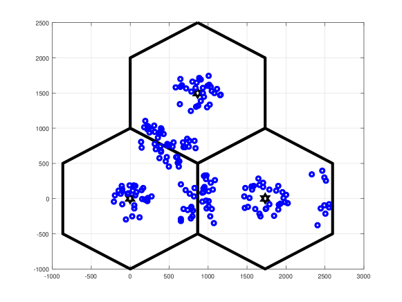
Figure 1: An equally mixed-coupled three-cell scenario. Each cell has a total of 60 UEs.

The vector channel from BS $j$ to UE $(i,k)$ is modelled by $\sqrt{\beta_{j,i,k}}\boldsymbol{h}_{{j,i,k}{}}$, where $\sqrt{\beta_{j,i,k}}$ models the path loss and large-scale fading, while [14, 18, 19]

$$\mathbf{h}_{j,i,k}=\mathbf{\Theta}_{j}^{1/2}\mathbf{h}_{j,i,k}^{w},$$ (1)

where $\mathbf{\Theta}_{j}\in\mathbb{C}^{N\times N}$ is a Hermitian symmetric positive semidefinite spatial correlation matrix of rank $r_{j}$ and $\mathbf{h}_{j,i,k}^{w}\in\mathbb{C}^{N}$ has independent and identical distributed complex entries of zero mean and unit variance, which represents the small-scale fading. The channel matrix from BS $j$ to UEs in $i$-th cell is thus $\beta_{j,i}\mathbf{H}^{H}_{j,i}$ where $\beta_{j,i}\triangleq\mbox{diag}[\sqrt{\beta_{j,i,k}}]_{k\in{\cal K}}$ and

$$\mathbf{H}^{H}_{j,i}\triangleq{\sf Col}[\mathbf{h}^{H}_{j,i,k}]_{k\in{\cal K}}.$$

Let $y_{i,k}\in\mathbb{C}$ be the signal received at UE $(i,k)$ and then $\mathbf{y}_{i}\triangleq{\sf Col}[y_{i,k}]_{k\in{\cal K}}$. The MIMO equation is thus

$$\mathbf{y}_{i} = \beta_{i,i}\mathbf{H}^{H}_{i,i}\mathbf{x}_{i}+\sum_{j\in{\cal I}\setminus\{i\}}\beta_{j,i}\mathbf{H}^{H}_{j,i}\mathbf{x}_{j}+\mathbf{n}_{i}$$ (2)

$$= \beta_{i,i}\mathbf{H}^{H}_{i,i}\mathbf{F}_{i}\mathbf{s}_{i}+\sum_{j\in{\cal I}\setminus\{i\}}\beta_{j,i}\mathbf{H}^{H}_{j,i}\mathbf{F}_{j}\mathbf{s}_{j}+\mathbf{n}_{i},$$ (3)

where $\mathbf{n}_{i}={\sf Col}[n_{i,k}]_{k\in{\cal K}}$ is the noise vector of independent entries $n_{i,k}\in{\cal CN}(0,\sigma^{2})$. Particularly, the multi-input single output (MISO) equation for the signal received at individual UE $(i,k)$ is

$$y_{i,k} =\sqrt{\beta_{i,i,k}}\underbrace{\boldsymbol{h}_{{i,i,k}{}}^{H}\boldsymbol{f}_{{i,k}{}}s_{i,k}}_{\text{desired signal}}+\underbrace{\sum_{\ell\in\mathcal{K}\setminus\{k\}}\sqrt{\beta_{i,i,k}}\boldsymbol{h}_{{i,i,k}{}}^{H}\boldsymbol{f}_{{i,\ell}{}}s_{i,\ell}}_{\text{inter-user interference}}+\underbrace{\sum_{j\in{\cal I}\setminus\{i\}}\sqrt{\beta_{j,i,k}}\mathbf{h}^{H}_{j,i,k}\mathbf{F}_{j}\mathbf{s}_{j}}_{\text{inter-cell interference}}+n_{i,k}.$$ (4)

We seek a beamforming matrix $\mathbf{F}_{i}$ in the following class

$$\mathbf{F}_{i}=\bar{\mathbf{F}}_{i}\mbox{diag}[\sqrt{p_{i,k}}]_{k\in{\cal K}}$$ (5)

with a predetermined matrix

$$\bar{\mathbf{F}}_{i}\triangleq{\sf Row}[\bar{\mathbf{f}}_{i,k}]_{k\in{\cal K}}\in\mathbb{C}^{N\times 2M}.$$ (6)

For $\mathbf{p}_{i}={\sf Col}[p_{i,k}]_{i\in{\cal K}}$ and $\mathbf{p}=(\mathbf{p}_{i})_{i\in{\cal I}}$, the inter-user interference and inter-cell interference functions are respectively defined from (4) as

$$\sigma_{i,k}^{\sf U}(\mathbf{p}_{i})\triangleq\beta_{i,i,k}\sum_{\ell\in\mathcal{K}\setminus\{k\}}|\boldsymbol{h}_{{i,i,k}{}}^{H}\bar{\mathbf{f}}_{i,\ell}|^{2}p_{i,\ell},$$ (7)

and

$$\sigma_{i,k}^{\sf C}(\mathbf{p})\triangleq\beta_{j,i,k}\sum_{j\in{\cal I}\setminus\{i\}}\sum_{\ell\in\mathcal{K}}||\bar{\mathbf{f}}_{j,\ell}||^{2}p_{j,\ell}.$$ (8)

Note that while the intra-cell channel $\boldsymbol{h}_{{i,i,k}{}}$ can be efficiently estimated [19], the intercell-channel $\boldsymbol{h}_{{j,i,k}{}}$ in (4) cannot be estimated and must be defined as in (8). Under the definitions

$$\alpha_{i,k}\triangleq\beta_{i,i,k}|\boldsymbol{h}_{{i,i,k}{}}^{H}\bar{\mathbf{f}}_{i,k}|^{2}$$ (9)

and

$$\lambda_{i,k}(\mathbf{p})\triangleq\sigma_{i,k}^{\sf U}(\mathbf{p}_{i})+\sigma_{i,k}^{\sf C}(\mathbf{p}),$$ (10)

which is a linear function, the information throughput at UE $(i,k)$ is defined by

$$r_{i,k}(\mathbf{p})=\ln\left(1+\frac{\alpha_{i,k}p_{i,k}}{\lambda_{i,k}(\mathbf{p})+\sigma^{2}}\right).$$ (11)

The transmit power by BS $i$ is the following function, which is also linear in $\mathbf{p}_{i}$:

$$\chi_{i}(\mathbf{p}_{i})=\sum_{k\in{\cal K}}||\bar{\mathbf{f}}_{i,k}||^{2}p_{i,k}.$$ (12)

The entire power consumption for the downlink transmission, which is expressed by

$$\pi(\mathbf{p})=\sum_{i\in{\cal I}}(\alpha\chi_{i}(\mathbf{p}_{i})+NP_{a}+P_{c})$$ (13)

is an affine function in $\mathbf{p}$. Here $\alpha>1$ is the reciprocal of the drain efficiency of the amplifier of BS and $P_{a}$ and $P_{c}$ are circuit power per antenna and non-transmission power of the BSs.

The network total throughput is defined as

$$\varphi(\mathbf{p})\triangleq\displaystyle\sum_{(i,k)\in{\cal I}\times{\cal K}}r_{i,k}(\mathbf{p}).$$

In this paper, we are interested in the following EE maximization problem under QoS constraints and power budgets:

$$\displaystyle\max_{\mathbf{p}}\ \varphi(\mathbf{p})/\pi(\mathbf{p})\quad\mbox{s.t.}$$ (14a)

$$\chi_{i}(\mathbf{p}_{i})\leq P_{i}^{\max},i\in{\cal I},$$ (14b)

$$r_{i,k}(\mathbf{p})\geq\bar{r}_{i,k},(i,k)\in{\cal I}\times{\cal K},$$ (14c)

where constraints (14c) set the QoS in terms of the throughput thresholds at each UE and constraint (14b) keeps the sum of transmit power under predefined budgets.

From definition (11) of $r_{i,k}(\mathbf{p})$, constraint (14c) is equivalent to the linear constraint

$$\alpha_{i,k}p_{i,k}\geq(e^{\bar{r}_{i,k}}-1)(\lambda_{i,k}(\mathbf{p})+\sigma^{2}),(i,k)\in{\cal I}\times{\cal K},$$ (15)

so (14) is a linear-constrained optimization problem. To obtain a path-following algorithm for solution of (14), it is most natural to iteratively approximate its objective by a lower bounding concave function (see e.g. [20, 21, 22]). We now propose a new and simpler approach, which involves a lower bounding approximation for the function in the numerator of the objective in (14) only but nevertheless also leads to a path-following computational procedure.

Let $\mathbf{p}^{(n)}$ be a feasible point for (14) found from the $(n-1)$th iteration and

$$t^{(n)}\triangleq\varphi(\mathbf{p}^{(n)})/\pi(\mathbf{p}^{(n)}),$$

so

$$\varphi(\mathbf{p}^{(n)})-t^{(n)}\pi(\mathbf{p}^{(n)})=0.$$ (16)

Using inequality (73) in the Appendix for

$$x=\alpha_{i,k}p_{i,k},y=\lambda_{i,k}(\mathbf{p})+\sigma^{2},$$

and

$$\bar{x}=\alpha_{i,k}p_{i,k}^{(n)},\bar{y}=\lambda_{i,k}(\mathbf{p}^{(n)})+\sigma^{2},$$

yields the following lower bounding approximation:

$$\varphi(\mathbf{p})\geq\varphi^{(n)}(\mathbf{p})$$

for

$$\varphi^{(n)}(\mathbf{p})\triangleq\displaystyle\sum_{(i,k)\in{\cal I}\times{\cal K}}\left(\bar{a}_{i,k}^{(n)}-\bar{b}_{i,k}^{(n)}/\alpha_{i,k}p_{i,k}-\bar{c}_{i,k}^{(n)}(\lambda_{i,k}(\mathbf{p})+\sigma^{2})\right),$$ (17)

where

$$\begin{array}[]{c}0<\bar{a}_{i,k}^{(n)}\triangleq\displaystyle r_{i,k}(\mathbf{p}^{(n)})+2\alpha_{i,k}p_{i,k}^{(n)}/\left(\lambda_{i,k}(\alpha_{i,k}p_{i,k}^{(n)}+\mathbf{p}_{i,k}^{(n)})+\sigma^{2}\right),\\ 0<\bar{b}_{i,k}^{(n)}\triangleq\displaystyle(\alpha_{i,k}p_{i,k}^{(n)})^{2}/\left(\alpha_{i,k}p_{i,k}^{(n)}+\lambda_{i,k}(\mathbf{p}_{i,k}^{(n)})+\sigma^{2}\right),\\ 0<\bar{c}_{i,k}^{(n)}\triangleq\displaystyle\alpha_{i,k}p_{i,k}^{(n)}/\left(\alpha_{i,k}p_{i,k}^{(n)}+\lambda_{i,k}(\mathbf{p}_{i,k}^{(n)})+\sigma^{2}\right)(\lambda_{i,k}(\mathbf{p}^{(n)})+\sigma^{2}).\end{array}$$ (18)

At the $n$th iteration, the following convex optimization subproblem is solved to generate the next feasible point $\mathbf{p}^{(n+1)}$ for (14):

$$\max_{\mathbf{p}}\left[\varphi^{(n)}(\mathbf{p})-t^{(n)}\pi(\mathbf{p})\right]\quad\mbox{s.t.}\quad(\ref{optb}),(\ref{g1ca}).$$ (19)

Note that $\mathbf{p}^{(n)}$ is a feasible point for (19) satisfying (16). Therefore, as far as $\mathbf{p}^{(n+1)}\neq\mathbf{p}^{(n)}$ we have

$$\begin{array}[]{lll}\varphi^{(n)}(\mathbf{p}^{(n+1)})-t^{(n)}\pi(\mathbf{p}^{(n+1)})&>&\varphi^{(n)}(\mathbf{p}^{(n)})-t^{(n)}\pi(\mathbf{p}^{(n)})\\ &=&\varphi(\mathbf{p}^{(n)})-t^{(n)}\pi(\mathbf{p}^{(n)})\\ &=&0,\end{array}$$

which implies

$$t^{(n+1)}\triangleq\varphi^{(n)}(\mathbf{p}^{(n+1)})/\pi(\mathbf{p}^{(n+1)})>t^{(n)},$$ (20)

i.e. $\mathbf{p}^{(n+1)}$ is a better feasible point than $\mathbf{p}^{(n)}$ for (14). Similarly to [23, Prop.1] it can be easily shown that at least, Algorithm 1 converges to a locally optimal solution of (49) satisfying the KKT conditions of optimality.

Algorithm 1 : Path-following algorithm for solving problem (14)

1:Initialization: Solve the following convex optimization problem

$$\min_{\mathbf{p}}\max_{i\in{\cal I}}[\chi_{i}(\mathbf{p}_{i})/P_{i}^{\max}]\quad\mbox{s.t.}\quad(\ref{g1ca}).$$ (21)

Exit if its optimal value is more than $1$ because it means that problem (14) is infeasible. Otherwise, take its optimal solution as a feasible point $\mathbf{p}^{(0)}$ for the convex constraints (14b), (15) and set $n:=0$ and $t^{(0)}=\varphi(\mathbf{p}^{(0)})/\pi(\mathbf{p}^{(0)})$.

2:Repeat

3:Solve problem (19) for its optimal solution $\mathbf{p}^{(n+1)}$. Set $t^{(n+1)}=\varphi(\mathbf{p}^{(n+1)})/\pi(\mathbf{p}^{(n+1)})$.

4:Set $n:=n+1$.

5:Until convergence of the objective in (14).

II-A Zero-forcing and regularized zero-forcing beamforming

In ZF beamforming, the matrix $\bar{\mathbf{F}}_{i}$ in (5) is the right inverse of the channel matrix $\mathbf{H}_{i,i}^{H}$:

$$\bar{\boldsymbol{F}}_{i}={\sf Row}[\bar{\mathbf{f}}_{i,k}]_{k\in{\cal K}}=\boldsymbol{H}_{i,i}(\boldsymbol{H}_{i,i}^{H}\boldsymbol{H}_{i,i})^{-1},$$ (22)

which exists only when $\boldsymbol{H}_{i,i}^{H}\boldsymbol{H}_{i,i}$ is nonsingular, particularly requiring $N>N_{UE}$. It can be seen that

$$\beta_{i,i}\mathbf{H}^{H}_{i,i}\mathbf{F}_{i}=\beta_{i,i}\mathbf{H}^{H}_{i,i}\boldsymbol{H}_{i,i}(\boldsymbol{H}_{i,i}^{H}\boldsymbol{H}_{i,i})^{-1}\mbox{diag}[\sqrt{p_{i,k}}]_{k\in{\cal K}}=\mbox{diag}[\sqrt{\beta_{i,i,k}}\sqrt{p_{i,k}}]_{k\in{\cal K}}$$

and thus the inter-user interference $\sigma^{\sf U}_{i,k}(\mathbf{p}_{i})$ in (4) is forced to zero. As such, $\alpha_{i,k}$ defined by (9) is $\beta_{i,i,k}$, while $\lambda_{i,k}(\mathbf{p})$ defined by (10) is

$$\lambda_{i,k}(\mathbf{p})=\sigma_{i,k}^{\sf C}(\mathbf{p})$$ (23)

with $\sigma_{i,k}^{\sf C}(\mathbf{p})$ defined from (8).

From (1) we also define $\mathbf{H}_{i,i}^{w}\triangleq[\mathbf{h}^{w}_{i,i,k}]_{k\in{\cal K}}$ so

$$\mathbf{H}_{i,i}=\mathbf{\Theta}_{i}^{1/2}\mathbf{H}^{w}_{i,i}$$

and $\mathbf{H}_{i,i}^{H}\mathbf{H}_{i,i}=(\mathbf{H}^{w}_{i,i})^{H}\mathbf{\Theta}_{i}\mathbf{H}^{w}_{i,i}$, which has rank not more than $r_{i}<N$. This makes matrix $(\mathbf{H}^{w}_{i,i})^{H}\mathbf{\Theta}_{i}\mathbf{H}^{w}_{i,i}$ quicker ill-conditioned as the number $N_{UE}$ of users increases. We now follow the regularization technique [11, 24] to consider the following class of RZF beamforming

$$\bar{\mathbf{F}}_{i}\triangleq\mathbf{H}_{i,i}(\mathbf{H}_{i,i}^{H}\mathbf{H}_{i,i}+\eta\mathbf{I}_{2M})^{-1},$$ (24)

with $\eta>0$. The optimal $\eta$ is not known and we just follow [11, 24, 25] to choose

$$\eta={2M}\sigma^{2}/P_{i}^{\max}.$$ (25)

Then

$$\beta_{i,i}\mathbf{H}_{i,i}^{H}\bar{\mathbf{F}}_{i}\mbox{diag}[\sqrt{p_{i,k}}]_{k\in{\cal K}} = \beta_{i,i}\mathbf{H}_{i,i}^{H}\mathbf{H}_{i,i}(\mathbf{H}_{i,i}^{H}\mathbf{H}_{i,i}+\eta\mathbf{I}_{2M})^{-1}\mbox{diag}[\sqrt{p_{i,k}}]_{k\in{\cal K}}$$ (26)

$$= \beta_{i,i}\mbox{diag}[\sqrt{p_{i,k}}]_{k\in{\cal K}}-\eta\beta_{i,i}(\mathbf{H}_{i,i}^{H}\mathbf{H}_{i,i}+\eta\mathbf{I}_{2M})^{-1}\mbox{diag}[\sqrt{p_{i,k}}]_{k\in{\cal K}}$$

$$= \beta_{i,i}\mbox{diag}[\sqrt{p_{i,k}}]_{k\in{\cal K}}-\eta\beta_{i,i}\mathbf{G}_{i}(\eta)\mbox{diag}[\sqrt{p_{i,k}}]_{k\in{\cal K}}$$

for Hermitian symmetric positive definite matrix

$$\mathbf{G}_{i}(\eta)=\left[\begin{matrix}\mathbf{g}_{i,1}\cr...\cr\mathbf{g}_{i,2M}\end{matrix}\right]=\left[\begin{matrix}g_{i,1,1}&...&g_{i,1,2M}\cr...&...&...\cr g_{i,2M,1}&...&g_{i,2M,2M}\end{matrix}\right]=(\mathbf{H}_{i,i}^{H}\mathbf{H}_{i,i}+\eta\mathbf{I}_{2M})^{-1}.$$ (27)

The inter-user interference $\sigma^{\sf U}_{i,k}(\mathbf{p}_{i})$ defined by (7) is

$$\sigma^{\sf U}_{i,k}(\mathbf{p}_{i})=\eta^{2}\beta_{i,k}\sum_{\ell\in{\cal K}\setminus\{k\}}|g_{i,k,\ell}|^{2}p_{i,\ell},$$ (28)

and the transmit power function defined by (12) is defined accordingly.

II-B Cell-wide zero-forcing beamforming (CWZF)

The design of cell-wide ZF (CWZF) beamforming is to ignore the multi-cell interference (8), i.e. it aims at optimizing

$$r_{i,k}(p_{i,k})=\ln\left(1+\beta_{i,i,k}p_{i,k}/\sigma^{2}\right).$$ (29)

For simplicity of presentation, in this subsection only we use the notation

$$\beta_{i,i,k}\rightarrow\bar{\beta}_{i,k}.$$ (30)

Accordingly, CWZF targets the following individual EE maximization problems for cells $i\in{\cal I}$, ignoring the intercell-interference (8):

$$\displaystyle\max_{\mathbf{p}_{i}} \quad\displaystyle\frac{\sum_{k\in{\cal K}}\ln\left(1+\bar{\beta}_{i,k}p_{i,k}/\sigma^{2}\right)}{\pi_{i}(\mathbf{p}_{i})}$$ (31a)

s.t. $$\quad\sum_{k\in{\cal K}}||\bar{\mathbf{f}}_{i,k}||^{2}p_{i,k}\leq P_{i}^{\text{max}}\,,$$ (31b)

$$\quad\ln\left(1+\bar{\beta}_{i,k}p_{i,k}/\sigma^{2}\right)\geq\hat{r}_{i,k},\,k\in{\cal K},$$ (31c)

where $\hat{r}_{i,k}$ is set to be $\hat{r}_{i,k}>\bar{r}_{i,k}$ to compensate the performance loss in the real performance caused by ignoring the intercell-interference (8).

Our conference paper [10] proposed the following treatment for (31). First, it follows from (31c) that

$$p_{i,k}\geq\bar{p}_{i,k}:=\sigma^{2}(e^{\hat{r}_{i,k}}-1)/\bar{\beta}_{i,k},$$

By making variable change

$$p_{i,k}=\tilde{p}_{i,k}+\bar{p}_{i,k}$$

it is straightforward to solve (31) by Dinkelbach’s type algorithm, which seeks $t>0$ such that the optimal solution of the following optimization problem is zero:

$$\max_{\tilde{\mathbf{p}}_{i}}\ \sum_{k\in{\cal K}}\ln\left(a_{i,k}+\bar{\beta}_{i,k}\tilde{p}_{i,k}/\sigma^{2}\right)-t\cdotp\tilde{\pi}_{i}(\tilde{\mathbf{p}}_{i})$$ (32a)

s.t. $$\sum_{k\in{\cal K}}||\bar{\mathbf{f}}_{i,k}||^{2}\tilde{p}_{i,k}\leq\bar{P}_{i}^{\text{max}}\,,\,\tilde{p}_{i,k}\geq 0\,,\,k\in{\cal K},$$ (32b)

where $a_{i,k}=1+\bar{\beta}_{i,k}\bar{p}_{i,k}/\sigma^{2}$, $\bar{P}_{i,\rm cir}=\alpha\sum_{k\in{\cal K}}||\bar{\mathbf{f}}_{i,k}||^{2}\bar{p}_{i,k}+P_{\rm cir}$, $P_{\rm cir}=NP_{a}+P_{c}$, $\bar{P}_{i}^{\rm max}=P_{i}^{\rm max}-\sum_{k\in{\cal K}}||\bar{\mathbf{f}}_{i,k}||^{2}\bar{p}_{i,k}$, $\tilde{\pi_{i}}(\tilde{\mathbf{p}}_{i})\triangleq\alpha\sum_{k\in{\cal K}}||\bar{\mathbf{f}}_{i,k}||^{2}\tilde{p}_{i,k}+\bar{P}_{i,\rm cir}$.
For $t>0$ fixed, problem (32) admits the optimal solution in closed-form:

$$\tilde{p}_{i,k}^{*}=\displaystyle\left[\frac{1}{||\bar{\mathbf{f}}_{i,k}||^{2}(t\alpha+\lambda)}-\frac{a_{i,k}\sigma^{2}}{\bar{\beta}_{i,k}}\right]^{+},k\in{\cal K}.$$ (33)

Here and after, $[x]^{+}=\max\{0,x\}$ and $\lambda=0$ whenever

$$\sum_{k\in{\cal K}}\left[\frac{1}{||\bar{\mathbf{f}}_{i,k}||^{2}t\alpha}-\frac{a_{i,k}\sigma^{2}}{\bar{\beta}_{i,k}}\right]^{+}\leq\bar{P}_{i}^{\text{max}}.$$

Otherwise, $\lambda>0$ is such that

$$\sum_{k\in{\cal K}}\left[\frac{1}{||\bar{\mathbf{f}}_{i,k}||^{2}(t\alpha+\lambda)}-\frac{a_{i,k}\sigma^{2}}{\bar{\beta}_{i,k}}\right]^{+}=\bar{P}_{i}^{\text{max}},$$ (34)

which can be easily located by the bisection search.

However, in contrast to [10], which uses bisection in locating the optimal $t$, we now propose a path-following Dinkelbach’s computational procedure for (31) as follow:

• Initialization. Solve (32) for $t=0$. Let $\tilde{\mathbf{p}}_{i}^{(opt)}$ be its optimal solution. Set

  $$\bar{t}=\sum_{k\in{\cal K}}\ln\left(a_{i,k}+\bar{\beta}_{i,k}\tilde{p}^{(opt)}_{i,k}/\sigma^{2}\right)/\tilde{\pi}_{i}(\tilde{\mathbf{p}}^{(opt)}_{i}).$$

• Solve (32) for $t=\bar{t}$ until its optimal value is zero. Let $\tilde{\mathbf{p}}_{i}^{(opt)}$ be its optimal solution. Reset $\bar{t}=\sum_{k\in{\cal K}}\ln\left(a_{i,k}+\bar{\beta}_{i,k}\tilde{p}^{(opt)}_{i,k}/\sigma^{2}\right)/\tilde{\pi}_{i}(\tilde{\mathbf{p}}^{(opt)}_{i})$.

III TF-wise zero-forcing and regularized zero-forcing beamforming

It can be seen from (8) that compared to the near UEs, the cell edge UEs suffer not only from worse channel conditions but also from the inter-cell interference, which cannot be forced to zero or mitigated. To tackle this issue of the intercell interference, we propose a scheme involving two separated transmissions within a time slot. During time-fraction $0\leq\tau_{1}\leq 1$, BS $1$ transmits signal to serve its near UEs while BS $2$ and BS $3$ transmit signals to serve their far UEs. During the remaining time-fraction $\tau_{2}=1-\tau_{1}$, BS $1$ transmits signal to serve its far UEs while BS $2$ and BS $3$ transmit signals to serve their near UEs. Under this time-fraction (TF)-wise scheme, the cell-edge UEs are almost free from the inter-cell interference because they are served by their BS when the neighbouring BSs serve their near UEs and thus need a very small transmission power that causes no interference to other cells. More importantly, this TF-wise scheme allows the individual BS to serve much larger numbers of UEs within the time slot.

Denote by ${\cal K}_{i,1}$ and ${\cal K}_{i,2}$ the set of those UEs in cell $i$, which are served during time-fraction $\tau_{1}$ and $\tau_{2}$, respectively. Under the proposed scheme,

$$\begin{array}[]{c}{\cal K}_{1,1}={\cal K}_{ne},{\cal K}_{1,2}={\cal K}_{fa},\\ {\cal K}_{i,1}={\cal K}_{fa},{\cal K}_{i,2}={\cal K}_{ne},i=2,3.\end{array}$$

The following definitions are used:

$$\begin{array}[]{c}\tau\triangleq(\tau_{1},\tau_{2}),\mathbf{s}_{i}^{[q]}\triangleq{\sf Col}[s_{i,k}]_{k\in{\cal K}_{i,q}},\mathbf{y}_{i}^{[q]}\triangleq{\sf Col}[y_{i,k}]_{k\in{\cal K}_{i,q}},\\ \mathbf{p}_{i}^{[q]}\triangleq{\sf Col}[p_{i,k}]_{k\in{\cal K}_{i,q}},\mathbf{p}^{[q]}=[\mathbf{p}_{i}^{s}]_{i\in{\cal I}},\mathbf{n}_{i}^{[q]}={\sf Row}[n_{i,k}]_{k\in{\cal K}_{i,q}},q=1,2;i\in{\cal I},\\ (\mathbf{H}^{[q]}_{j,i})^{H}\triangleq{\sf Col}[\mathbf{h}^{H}_{j,i,k}]_{k\in{\cal K}_{i,q}}.\end{array}$$ (35)

As mentioned before, the inter-cell interference is weak in this TF-wise beamforming and thus can be ignored. The MIMO equation of signal reception in time-fraction $\tau_{q}$ is thus

$$\mathbf{y}_{i}^{[q]}=\beta_{i,i}(\mathbf{H}^{[q]}_{i,i})^{H}\mathbf{F}_{i}^{[q]}\mathbf{s}_{i}^{[q]}+\mathbf{n}_{i}^{[q]}.$$ (36)

We seek $\mathbf{F}_{i}^{[q]}$ is the class of

$$\mathbf{F}_{i}^{[q]}=\bar{\mathbf{F}}_{i}^{[q]}\mbox{diag}[1/\sqrt{p_{i,k}}]_{k\in{\cal K}_{i,q}}$$ (37)

with predetermined $\bar{\mathbf{F}}_{i}^{[q]}\in\mathbf{C}^{N\times M}={\sf Row}[\bar{\mathbf{f}}_{i,k}]_{k\in{\cal K}_{i,q}}$.

The inter-user interference in time-fraction $\tau_{q}$ defined as

$$\sigma_{i,k}^{[q]}(\mathbf{p}_{i}^{[q]})=\beta_{i,i,k}\sum_{\ell\in\mathcal{K}_{i,q}\setminus\{k\}}|\mathbf{h}_{i,i,k}^{H}\bar{\mathbf{f}}_{i,\ell}|^{2}/p_{i,\ell},\ell\in{\cal K}_{i,q},$$ (38)

which is a convex function in $\mathbf{p}_{i}^{[q]}$.

The information throughput at UE $(i,k)$, $k\in{\cal K}_{i,q}$ is $\tau_{q}r^{[q]}_{i,k}(\mathbf{p}_{i}^{[q]})$ with

$$r^{[q]}_{i,k}(\mathbf{p}_{i}^{[q]})\triangleq\ln\left(1+\frac{\beta_{i,i,k}|\boldsymbol{h}_{{i,i,k}{}}^{H}\bar{\mathbf{f}}_{i,k}|^{2}/p_{i,k}}{\sigma_{i,k}^{[q]}(\mathbf{p}_{i}^{[q]})+\sigma^{2}}\right)=\ln\left(1+\frac{\alpha_{i,k}/p_{i,k}}{\sigma_{i,k}^{[q]}(\mathbf{p}_{i}^{[q]})+\sigma^{2}}\right)$$ (39)

for

$$\alpha_{i,k}\triangleq\beta_{i,i,k}|\boldsymbol{h}_{{i,i,k}{}}^{H}\bar{\mathbf{f}}_{i,k}|^{2}.$$ (40)

The transmit beamforming power during time-fraction $\tau_{q}$ of each cell is $\tau_{q}\chi_{i}^{[q]}(\mathbf{p}_{i}^{[q]})$ with

$$\chi_{i}^{[q]}(\mathbf{p}_{i}^{[q]})\triangleq\sum_{k\in{\cal K}_{i,q}}||\bar{\mathbf{f}}_{i,k}||^{2}/p_{i,k},$$ (41)

which must satisfy the power constraint

$$\sum_{q=1}^{2}\tau_{q}\chi_{i}^{[q]}(\mathbf{p}_{i}^{[q]})\leq P_{i}^{\max},i\in{\cal I}.$$ (42)

We also impose additionally the following physical constraints

$$||\bar{\mathbf{f}}_{i,k}||^{2}/3P_{i}^{\max}\leq p_{i,k},(i,k)\in{\cal I}\times{\cal K}$$ (43)

to substance the fact that it is not possible to transmit an arbitrary high power during time-fractions.
The entire power consumption for the downlink transmission is expressed by

$$\pi(\tau,\mathbf{p})=\sum_{i\in{\cal I}}(\alpha\sum_{q=1}^{2}\tau_{q}\chi_{i}^{[q]}(\mathbf{p}_{i}^{[q]})+P_{\rm cir}).$$ (44)

The EE maximization problem under QoS constraints and power budget is now formulated as

$$\displaystyle\max_{\tau,\mathbf{p}} \displaystyle\frac{\sum_{q=1}^{2}\tau_{q}\sum_{i\in{\cal I}}\sum_{k\in{\cal K}_{i,q}}r^{[q]}_{i,k}(\mathbf{p}^{[q]}_{i})}{\pi(\tau,\mathbf{p})}\quad\mbox{s.t.}\quad(\ref{fpower2}),(\ref{fpower3}),$$ (45a)

$$\tau_{q}r^{[q]}_{i,k}(\mathbf{p}_{i}^{[q]})\geq\overline{r}_{i,k},\,i\in{\cal I},k\in{\cal K}_{i,q},q=1,2,$$ (45b)

$$\tau_{1}\geq 0,\tau_{2}\geq 0,\tau_{1}+\tau_{2}\leq 1.$$ (45c)

To address (45), introduce the new variable

$$\theta=(\theta_{1},\theta_{2}),$$ (46)

which satisfies the convex constraints

$$\tau\theta_{1}\geq 1,(1-\tau)\theta_{2}\geq 1,\theta_{1}>0,\theta_{2}>0.$$ (47)

The power constraint (42) is now

$$\Pi_{i}(\theta_{2},\mathbf{p}_{i})\triangleq(1-1/\theta_{2})\chi^{[1]}_{i}(\mathbf{p}_{i}^{[1]})+\chi^{[2]}_{i}(\mathbf{p}_{i}^{[2]})/\theta_{2}\leq P_{i}^{\max}.$$ (48)

Problem (45) is now expressed by

$$\displaystyle\max_{\tau,\theta,\mathbf{p}}\ \Phi(\theta,\mathbf{p})/\Pi(\theta_{2},\mathbf{p})\quad\mbox{s.t.}\quad(\ref{fpower3}),(\ref{cond_var_rzf_3cell}),(\ref{ad1_rzf_3cell}),$$ (49a)

$$\displaystyle r^{[q]}_{i,k}(\mathbf{p}_{i}^{[q]})/\theta_{q}\geq\bar{r}_{i,k},q=1,2;i\in{\cal I};k\in{\cal K}_{i,q},$$ (49b)

where

$$\Phi(\theta,\mathbf{p})\triangleq\displaystyle\sum_{q=1}^{2}\frac{1}{\theta_{q}}\sum_{i\in{\cal I}}\sum_{k\in\mathcal{K}_{i,q}}r^{[q]}_{i,k}(\mathbf{p}_{i}^{[q]})$$

and

$$\Pi(\theta_{2},\mathbf{p})=\sum_{i\in{\cal I}}\left(\alpha\cdot\Pi_{i}(\theta_{2},\mathbf{p}_{i})+P_{\rm cir}\right).$$

Let $(\tau^{(n)},\theta^{(n)},\mathbf{p}^{(n)})$ be a feasible point for (49) found from the $(n-1)$th iteration and

$$t^{(n)}=\Phi(\theta^{(n)},\mathbf{p}^{(n)})/\Pi(\theta_{2}^{(n)},\mathbf{p}^{(n)}).$$

By using inequality (74) in the Appendix,

$$\Pi_{i}(\theta_{2},\mathbf{p}_{i})\leq\Pi_{i}^{(n)}(\theta_{2},\mathbf{p}_{i})$$ (50)

for the convex function

$$\Pi_{i}^{(n)}(\theta_{2},\mathbf{p}_{i})\triangleq\chi^{[1]}_{i}(\mathbf{p}_{i}^{[1]})+\chi^{[2]}_{i}(\mathbf{p}_{i}^{[2]})/\theta_{2}+\sum_{k\in{\cal K}_{i,1}}||\bar{\mathbf{f}}_{i,k}||^{2}\left(p_{i,k}/p^{(n)}_{i,k}+\theta_{2}/\theta_{2}^{(n)}-3\right)/p^{(n)}_{i,k}\theta_{2}^{(n)}.$$ (51)

Therefore, the nonconvex constraint (48) is innerly approximated by the convex constraint

$$\Pi_{i}^{(n)}(\theta_{2},\mathbf{p}_{i})\leq P^{\max}_{i},i\in{\cal I}.$$ (52)

To innerly approximate the nonconvex constraint (49b) in (49), we apply inequality (72) in the Appendix for

$$x=p_{i,k}/\alpha_{i,k},\ y=\sigma_{i,k}^{[q]}(\mathbf{p}_{i}^{[q]})+\sigma^{2},$$

and

$$\bar{x}=p_{i,k}^{(n)}/\alpha_{i,k},\bar{y}=\sigma_{i,k}^{[q]}(\mathbf{p}_{i}^{q,(n)})+\sigma^{2},$$

to obtain

$$r^{[q]}_{i,k}(\mathbf{p}_{i}^{[q]})\geq r_{i,k}^{q,(n)}(\mathbf{p}_{i}^{[q]})$$ (53)

for

$$r_{i,k}^{q,(n)}(\mathbf{p}_{i}^{[q]})=\bar{a}_{i,k}^{(n)}-\bar{b}_{i,k}^{(n)}p_{i,k}/\alpha_{i,k}-\bar{c}_{i,k}^{(n)}(\sigma_{i,k}^{[q]}(\mathbf{p}_{i}^{[q]})+\sigma^{2}),$$ (54)

where

$$\begin{array}[]{c}0<\bar{a}_{i,k}^{(n)}\triangleq\displaystyle r^{[q]}_{i,k}(\mathbf{p}_{i}^{q,(n)})+2\alpha_{i,k}/\left(p_{i,k}^{(n)}(\sigma_{i,k}^{[q]}(\mathbf{p}_{i}^{q,(n)})+\sigma^{2})+\alpha_{i,k}\right),\\ 0<\bar{b}_{i,k}^{(n)}\triangleq\displaystyle(\alpha_{i,k})^{2}/\left(p_{i,k}^{(n)}(\sigma_{i,k}^{[q]}(\mathbf{p}_{i}^{q,(n)})+\sigma^{2})+\alpha_{i,k}\right)p_{i,k}^{(n)},\\ 0<\bar{c}_{i,k}^{(n)}\triangleq\displaystyle\alpha_{i,k}/\left(p_{i,k}^{(n)}(\sigma_{i,k}^{[q]}(\mathbf{p}_{i}^{q,(n)})+\sigma^{2})+\alpha_{i,k}\right)(\sigma_{i,k}^{[q]}(\mathbf{p}_{i}^{q,(n)})+\sigma^{2}).\end{array}$$ (55)

The nonconvex constraint (49b) is thus innerly approximated by the following convex constraint:

$$r_{i,k}^{q,(n)}(\mathbf{p}_{i}^{[q]})\geq\theta_{q}\overline{r}_{i,k}\,,\,q=1,2;i\in{\cal I},k\in{\cal K}_{i,q}.$$ (56)

Next, we address the terms in the numerator of the objective in (49a). By using inequality (71) in the Appendix for

$$x=p_{i,k}/\alpha_{i,k},\ y=\sigma_{i,k}^{[q]}(\mathbf{p}_{i}^{[q]})+\sigma^{2},t\triangleq\theta_{q},$$

and

$$\bar{x}=p_{i,k}^{(n)}/\alpha_{i,k},\bar{y}=\sigma_{i,k}^{[q]}(\mathbf{p}_{i}^{q,(n)})+\sigma^{2},\bar{t}=\theta_{q}^{(n)},$$

we obtain

$$r^{[q]}_{i,k}(\mathbf{p}_{i}^{[q]})/\theta_{q}\geq g_{i,k}^{q,(n)}(\theta_{q},\mathbf{p}),$$ (57)

where

$$g_{i,k}^{q,(n)}(\theta_{q},\mathbf{p})\triangleq a_{i,k}^{(n)}-b_{i,k}^{(n)}p_{i,k}/\alpha_{i,k}-c_{i,k}^{(n)}(\sigma_{i,k}^{[q]}(\mathbf{p}_{i}^{[q]})+\sigma^{2})-d_{i,k}^{(n)}\theta_{q}$$ (58)

with

$$\begin{array}[]{lll}0<a_{i,k}^{(n)}&\triangleq&2r_{i,k}(\mathbf{p}_{i}^{q,(n)})/\theta_{q}^{(n)}+2\alpha_{i,k}/\left(p_{i,k}^{(n)}(\sigma_{i,k}^{[q]}(\mathbf{p}_{i}^{q,(n)})+\sigma^{2})+\alpha_{i,k}\right)\theta_{q}^{(n)},\\ 0<b_{i,k}^{(n)}&\triangleq&\displaystyle(\alpha_{i,k})^{2}/\left(p_{i,k}^{(n)}(\sigma_{i,k}^{[q]}(\mathbf{p}_{i}^{q,(n)})+\sigma^{2})+\alpha_{i,k}\right)p_{i,k}^{(n)}\theta_{q}^{(n)},\\ 0<c_{i,k}^{(n)}&\triangleq&\displaystyle\alpha_{i,k}/\left(p_{i,k}^{(n)}(\sigma_{i,k}^{[q]}(\mathbf{p}_{i}^{q,(n)})+\sigma^{2})+\alpha_{i,k}\right)(\sigma_{i,k}^{[q]}(\mathbf{p}_{i}^{q,(n)})+\sigma^{2})\theta_{q}^{(n)},\\ 0<d_{i,k}^{(n)}&\triangleq&r_{i,k}(\mathbf{p}_{i}^{q,(n)})/(\theta_{q}^{(n)})^{2}.\end{array}$$ (59)

At the $n$th iteration, the following convex program is solved to generate the next feasible point $(\tau^{(n+1)},\theta^{(n+1)},\mathbf{p}^{(n+1)})$ for (49):

$$\displaystyle\max_{\theta,\tau,\mathbf{p}}\ \displaystyle\sum_{q=1}^{2}\sum_{i\in{\cal I}}\sum_{k\in{\cal K}_{i,q}}g_{i,k}^{q,(n)}(\theta_{q},\mathbf{p})-t^{(n)}\sum_{i\in{\cal I}}\left(\alpha\cdot\Pi_{i}^{(n)}(\theta_{2},\mathbf{p}_{i})+P_{\rm cir}\right)$$

$$\mbox{s.t.}\quad(\ref{fpower3}),(\ref{cond_var_rzf_3cell}),(\ref{fopt3}),(\ref{cond_rate_1_rzf_3cell}).$$ (60)

In Algorithm 2, we propose a path-following computational procedure for the EE maximization problem (49).

To find an initial point $(\theta^{(0)},\mathbf{p}^{(0)})$ for (49) we fix $\theta^{(0)}$ such that it satisfies (47), and solve the following linear programming problem:

$$\displaystyle\min_{\mathbf{p}}\ \tilde{\pi}(\mathbf{p})\quad\mbox{s.t.}\quad\tilde{\pi}_{i}(\mathbf{p}_{i})\leq P_{i}^{\max},i\in{\cal I},$$ (61a)

$$\displaystyle\alpha_{i,k}p_{i,k}\geq(e^{\theta_{q}^{(0)}\overline{r}_{i,k}}-1)(\tilde{\sigma}_{i,k}^{[q]}(\mathbf{p}_{i}^{[q]})+\sigma^{2}),q=1,2;i\in{\cal I},k\in{\cal K}_{i,q},$$ (61b)

where

$$\begin{array}[]{c}\tilde{\pi}_{i}(\mathbf{p}_{i})\triangleq\displaystyle(1-\frac{1}{\theta_{2}^{(0)}})\sum_{k\in{\cal K}_{i,1}}||\bar{\mathbf{f}}_{i,k}||^{2}p_{i,k}+\sum_{k\in{\cal K}_{i,2}}||\bar{\mathbf{f}}_{i,k}||^{2}p_{i,k},i\in{\cal I},\\ \tilde{\pi}(\mathbf{p})\triangleq\sum_{i\in{\cal I}}\tilde{\pi}_{i}(\mathbf{p}_{i}),\\ \tilde{\sigma}_{i,k}^{[q]}(\mathbf{p}_{i}^{[q]})\triangleq\beta_{i,i,k}\sum_{\ell\in\mathcal{K}_{i,q}\setminus\{k\}}|\mathbf{h}_{i,i,k}^{H}\bar{\mathbf{f}}_{i,\ell}|^{2}p_{i,k},k\in{\cal K}_{i,q},\end{array}$$

which are linear functions. Note that the linear constraint (61b) represents the following QoS constraints

$$\frac{1}{\theta_{q}^{(0)}}\ln\left(1+\frac{\alpha_{i}p_{i,k}}{\tilde{\sigma}_{i,k}^{[q]}(\mathbf{p}_{i}^{[q]})+\sigma^{2}}\right)\geq\overline{r}_{i,k},q=1,2;i\in{\cal I},k\in{\cal K}_{i,q}.$$ (62)

Suppose $\bar{\mathbf{p}}$ is the optimal solution of (61). Then an initial point $(\theta^{(0)},\mathbf{p}^{(0)})$ for (49) is $p^{(0)}_{i,k}=1/\bar{p}_{i,k}$.

Algorithm 2 : Path-following algorithm for solving problem (49)

1:Initialization: Solve (61) to take its optimal solution as a feasible point $(\theta^{(0)},\mathbf{p}^{(0)})$ for (49). Set $n:=0$ and $t^{(0)}:=\Phi(\theta^{(0)},\mathbf{p}^{(0)})/\Pi(\theta_{2}^{(0)},\mathbf{p}^{(0)})$.

2:Repeat

3: Solve the problem (III) for its optimal solution $(\tau^{(n+1)},\theta^{(n+1)},\mathbf{p}^{(n+1)})$. Set $t^{(n+1)}:=\Phi(\theta^{(n+1)},\mathbf{p}^{(n+1)})/\Pi(\theta_{2}^{(n+1)},\mathbf{p}^{(n+1)})$.

4:Set $n:=n+1$.

5:Until convergence of the objective in (49).

Similar to Algorithm 1, at least Algorithm 2 converges to a locally optimal solution of (49) satisfying the KKT conditions of optimality.

For TF-wise ZF beamforming, $\bar{\mathbf{F}}^{[q]}_{i}$ in (37) is the right inverse of the matrix $(\mathbf{H}^{[q]}_{i,i})^{H}$:

$$\bar{\boldsymbol{F}}^{[q]}_{i}={\sf Col}[\bar{\mathbf{f}}_{i,k}]_{k\in{\cal K}_{i,q}} =\boldsymbol{H}^{[q]}_{i,i}((\boldsymbol{H}^{[q]}_{i,i})^{H}\boldsymbol{H}^{[q]}_{i,i})^{-1}.$$ (63)

under which the inter-user interference $\sigma_{i,k}^{q}(\mathbf{p}_{i}^{[q]})$ in (38) is zero.

On the other hand, for TF-wise RZF beamforming, $\bar{\mathbf{F}}^{[q]}_{i}$ in (37) is

$$\bar{\mathbf{F}}^{q}_{i}=\mathbf{H}^{[q]}_{i,i}((\mathbf{H}^{[q]}_{i,i})^{H}\mathbf{H}^{[q]}_{i,i}+\eta\mathbf{I}_{M})^{-1}.$$ (64)

with

$$\eta={M}\sigma^{2}/P_{i}^{\max}.$$ (65)

Then

$$\beta_{i,i}(\mathbf{H}^{[q]}_{i,i})^{H}\mathbf{F}_{i}^{[q]} = \beta_{i,i}\mbox{diag}[\sqrt{p_{i,k}}]_{k\in{\cal K}_{i,q}}-\eta\beta_{i,i}\mathbf{G}^{[q]}_{i}(\eta)\mbox{diag}[1/\sqrt{p_{i,k}}]_{k\in{\cal K}_{i,q}}$$ (66)

for the Hermitian symmetric positive definite matrix

$$\mathbf{G}^{[q]}_{i}(\eta)=\left[\begin{matrix}\mathbf{g}^{[q]}_{i,1}\cr...\cr\mathbf{g}^{[q]}_{i,M}\end{matrix}\right]=\left[\begin{matrix}g_{i,1,1}&...&g_{i,1,M}\cr...&...&...\cr g_{i,M,1}&...&g_{i,M,M}\end{matrix}\right]=((\mathbf{H}^{[q]}_{i,i})^{H}\mathbf{H}^{[q]}_{i,i}+\eta\mathbf{I}_{M})^{-1}.$$ (67)

In this case, $\alpha_{i,k}$ defined by (40) is

$$\alpha_{i,k}=\beta_{i,k}(1-\eta g_{i,k,k})^{2},$$

while the inter-user interference $\sigma_{i,k}^{[q]}(\mathbf{p}_{i}^{[q]})$ in (38) is

$$\sigma_{i,k}^{[q]}(\mathbf{p}_{i}^{[q]})\triangleq\eta^{2}\beta_{i,k}\sum_{\ell\in{\cal K}_{i,q}\setminus\{k\}}|g_{i,k,\ell}|^{2}/p_{i,\ell},k\in{\cal K}_{i,q}.$$ (68)

The transmit power function $\chi_{i}^{[q]}(\mathbf{p}_{i}^{[q]})$ defined by (41) is also represented as

$$\chi_{i}^{[q]}(\mathbf{p}_{i}^{[q]})=\mbox{trace}\left(\mathbf{G}^{[q]}_{i}(\eta)(\mathbf{H}^{[q]}_{i,i})^{H}\mathbf{H}^{[q]}_{i,i}\mathbf{G}^{[q]}_{i}(\eta)\mbox{diag}[1/p_{i,k}]_{k\in{\cal K}_{i,q}}\right).$$ (69)

IV Numerical Simulations

In this section, we evaluate the performance of the proposed algorithms by numerical examples for different scenarios of single-cell, two-cell and three-cell networks. Unless otherwise stated, it is assumed that $N_{\sf ne}=N_{\sf fa}=N_{UE}/2$. The cell-edge UEs are equally distributed at the cell boundaries, while the near UEs are equally distributed nearly the BSs. Each of BSs is located at the centre of a hexagon cell with radius $1$ km and equipped with an $8\times 8$ uniform planar array (UPA) of antennas ($8$ rows in the horizontal dimension and $8$ columns in the vertical dimension). Thus, the total number of antennas at each BS is $N=64$. A popular model for the spatial correlation matrix $\Theta_{j}$ in (1) is an $2D$ extension [14, 18] of one ring model [13], which is of very low rank [19] under the standard assumption that antennas are a half-wavelength spaced to result in a form factor of $0.25$ m $\times$ $0.25$ m [26]. To investigate the impact of the spatial correlation to the number of UEs as well as the users’s QoS that massive MIMO can promise, we adopt the standard exponential correlation model, where the correlation between antenna $(p,q)$ and antenna $(m,n)$ is modelled by

$$[\mathbf{\Theta}]_{(p,q),(m,n)}=\rho^{|p-m|+|q-n|}$$ (70)

with $0<\rho<1$, which was also used e.g. in [27]. To study the effect of spatial correlation to capacity of massive MIMO, we consider two cases of $\rho=0.9$ and $\rho=0.5$, which correspond to high and medium spatial correlations.

Other simulation parameters for generating large scale fading in Table I are similar to those used in [28]. The throughput threshold for all users is set as $\bar{r}_{i,k}\equiv r\in\{0.4,1\}$ bps/Hz [29, Table I].

Table I: Large scale fading Setup

Parameter	Numerical value
Carrier frequency / Bandwidth	$2$GHz / $10$MHz
BS transmission power	$46$ dBm
Path loss from BS to UE	$128.1+37.6\operatorname{\mathrm{log}}_{10}R$ [dB], R in km
Shadowing standard deviation	$8$ dB
Noise power density	$-174$ dBm/Hz
Noise figure	$9$ dB
Drain efficiency of amplifier	$\alpha=1/0.388$
Circuit power per antenna	$P_{A}$ = $189$ mW
Non-transmission power	$P_{C}$ = $40$ dBm

IV-A Single-cell network

A typical convergence of the proposed Algorithm 1 for RZF beamforming, Dinkelbach’s type iterations for CWZF beamforming and Algorithm 2 for TF-based ZF and RZF beamforming is provided by Fig. 2, where all of them are seen to converge rapidly within several iterations. It is worthy to mention that the new path-following Dinkelbach’s iterations converge much more rapidly than that proposed in [10], which are based on bisection for locating the optimal value of $t$ in (32).

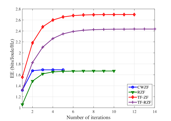
Figure 2: The convergence of CWZF, RZF, TF-ZF and TF-RZF vs. iteration number under $N_{\sf UE}=40$, $\rho=0.9$ and $r=0.4$ bps/Hz.

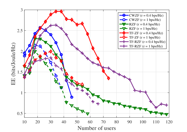
Figure 3: The EE performance in CWZF, RZF, TF-wise ZF and TF-wise RZF vs. the number of users under $\rho=0.9$ and $r\in\{0.4,1\}$ bps/Hz.

Fig. 3 plots the EE performance of the proposed beamforming approaches versus the number of users under $\rho=0.9$. RZF beamforming is always capable of serving a much larger numbers of UEs than ZF beamforming is. For the throughput threshold $r=0.4$ bps/Hz ($r=1$ bps/Hz, resp.), CWZF beamforming and TF-wise ZF beamforming cannot serve more than $46$ UEs ($38$ UEs, resp.) and $82$ UEs ($54$ UEs, resp.). Meanwhile, both RZF beamforming and TF-wise RZF beamforming can serve up to $120$ UEs ($66$ UEs, resp.) for $r=0.4$ bps/Hz ($r=1$ bps/Hz, resp.) but the latter clearly outperforms the former in term of EE. Note that both numbers $120$ and $66$ of the served UEs excess the number $64$ of BS’s antennas. Both optimal time-fraction allocation for two separated transmission within the time slot and optimal power allocation for beamformers enable massive MIMO to serve numbers of UEs that are larger than the number of transmit antennas.

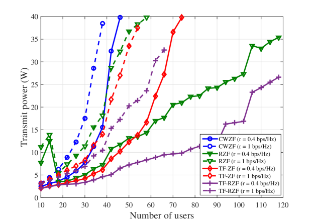
Figure 4: The transmit power in CWZF, RZF, TF-wise ZF and TF-wise RZF vs. the number of users under $\rho=0.9$ and $r\in\{0.4,1\}$ bps/Hz.

Furthermore, all EE performances increase quickly to a certain value of $N_{UE}$ and drop after that. Fig. 4 reveals that this drop is caused by the increased total transmit power. There is no magic number $N_{UE}$, under which all the EE performances attain their peak. Of course, increasing the throughput threshold from $0.4$ bps/Hz to $1$ bps/Hz leads to decreasing numbers of the served UEs and degrading EE performance. Fig. 4 also shows that TF-wise beamforming could manage the power control better than other beamforming schemes.

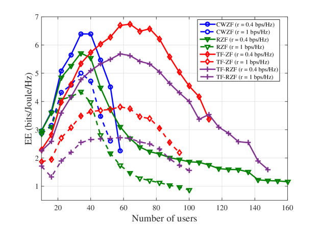
Figure 5: The EE performance in CWZF, RZF, TF-wise ZF and TF-wise RZF vs. the number of users under $\rho=0.5$ and $r=\{0.4,1\}$ bps/Hz.

Figure 6: The value of $\tau/(1-\tau)$ in TF-ZF and TF-RZF vs. the number of users.

Fig. 5 plots the EE performance of the proposed beamforming schemes under $\rho=0.5$. Lower spatial correlation obviously leads to not only better EE but also larger numbers of the served UEs. Specifically, the EE performance is doubly increased in all proposed beamforming schemes and TF-wise RZF beamforming can serve $160$ UEs vs $120$ UEs served under $\rho=0.9$.

Fig. 6 and Fig. 7 plot the ratio between time-fractions in serving the near UEs and the cell-edge UEs and the corresponding power ratio, which are monotonically decreased in the total number $N_{UE}$ of UEs. Recalling that $N_{\sf ne}=N_{\sf fa}=N_{UE}/2$ in our setting, at small $N_{UE}$ / small $N_{\sf fa}$ more time-fraction and power are allocated to the near UEs to maximize their throughput. On the other hand, at large $N_{UE}$ / large $N_{\sf fa}$, more time-fraction and power must be allocated to the far UEs in assuring their QoS.

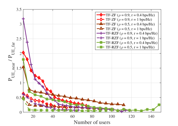
Figure 7: The ratio of transmit power for near UEs and far UEs in TF-ZF and TF-RZF vs. the number of users.

IV-B Two-cell network

The network is depicted by Fig. 8, where the cell-edge UEs are located at the boundary areas between the cells. Under the TF-wise beamforming schemes, during time-fraction $0\leq\tau\leq 1$, BS $1$ serves its near UEs while BS $2$ serves its cell-edge UEs. During the remaining fraction ($1-\tau$), BS $1$ serves its cell-edge UEs while BS $2$ serves its near UEs. The cell-edge UEs are thus free from the inter-cell interference.

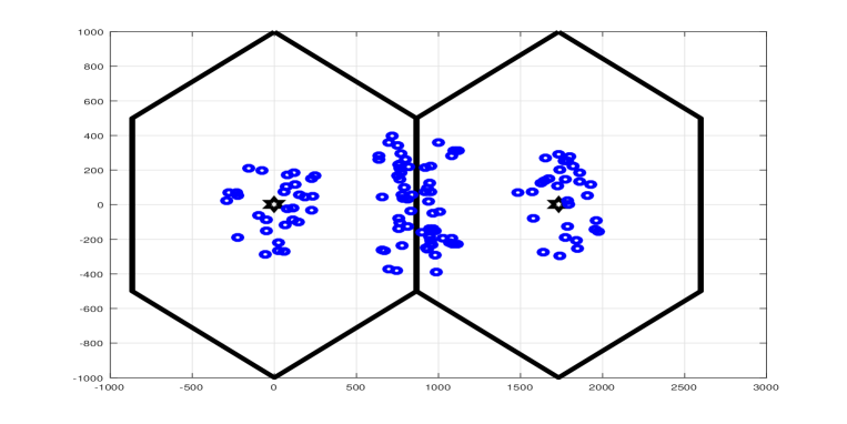
Figure 8: An equally mixed-coupled two-cell scenario. Each cell has a total of 60 UEs.

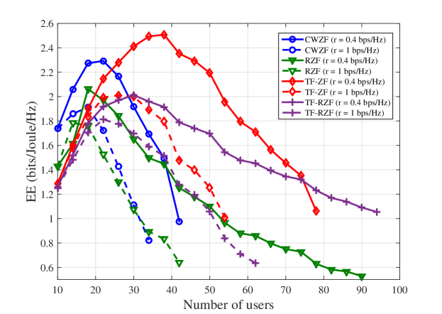
Figure 9: The EE performance in CWZF, RZF and TF vs. the number of users under $\rho=0.9$, $r\in\{0.4,1\}$ bps/Hz and $\hat{r}=\{0.6,1.4\}$ bps/Hz.

Fig. 9 and Fig. 10 show the superior performance of TF-wise beamforming schemes over others. For the throughput threshold $r=0.4$ bps/Hz, CWZF beamforming cannot serve more than $40$ UEs and $60$ UEs while TF-wise ZF beamforming still serves up to $80$ UEs and $120$ UEs, respectively. Under both spatial correlation degrees, RZF beamforming and TF-wise RZF beamforming can serve up to $90$ UEs and $150$ UEs but the latter significantly outperforms the former in term of EE. It is observed that the EE gap in assuring the throughput thresholds becomes wider as the number $N_{UE}$ of UEs increases.

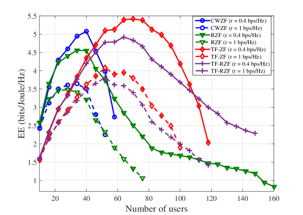
Figure 10: The EE performance in CWZF, RZF and TF vs. the number of users under $\rho=0.5$, $r\in\{0.4,1\}$ bps/Hz and $\hat{r}=\{0.6,1.4\}$ bps/Hz.

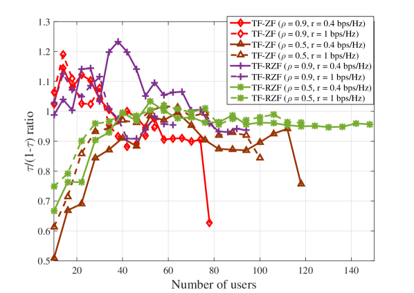
Figure 11: The value of $\tau/(1-\tau)$ vs. the number of users.

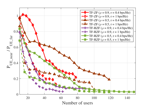
Figure 12: The total transmit power for near UEs and far UEs ratio vs. the number of users.

Interestingly, Fig. 11 and Fig. 12 show that the time-fraction allocation and power allocation in this two-cell case are quite different from that in the single-cell case. They are more or less balanced because the same numbers of cell-edge UEs and near UEs are served in different time-fractions.

IV-C Three-cell network

We return to a three-cell network illustrated by Fig. 1. Being free from inter-cell interference, TF-wise beamforming schemes can serve higher numbers of UEs with higher EE achieved, as Fig. 13 and Fig. 14 show. Particularly, TF-wise ZF beamforming and TF-wise RZF beamforming are able to serve at least $80$ UEs and $120$ UEs per cell for $\rho=0.9$ and $\rho=0.5$, respectively. Both RZF beamforming and TF-wise RZF beamforming can serve up to $150$ UEs for $\rho=0.5$ but the latter clearly outperform the former in terms of EE.

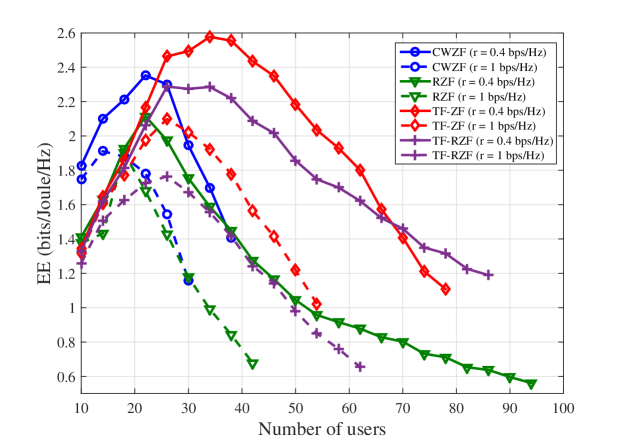
Figure 13: The EE performance in CWZF, RZF and TF vs. the number of users under $\rho=0.9$, $r=\{0.4,1\}$ bps/Hz and $\hat{r}=\{0.6,1.4\}$ bps/Hz.

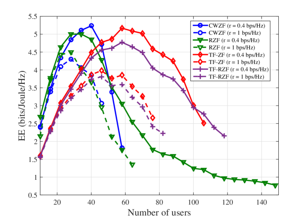
Figure 14: The EE performance in CWZF, RZF and TF vs. the number of users under $\rho=0.5$, $r=\{0.4,1\}$ bps/Hz and $\hat{r}=\{0.6,1.4\}$ bps/Hz.

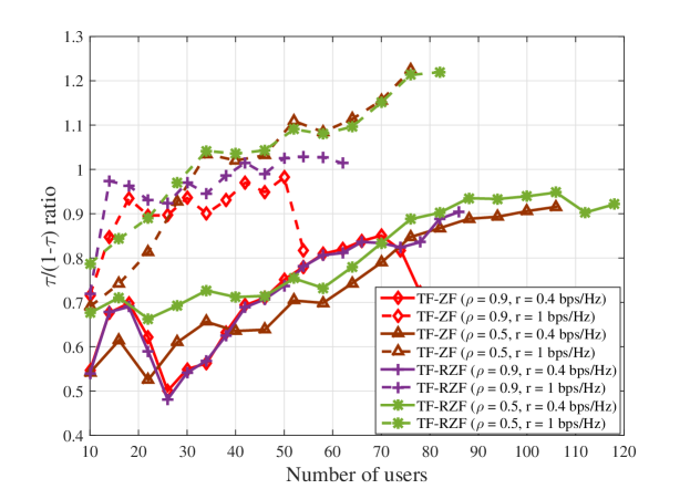
Figure 15: The value of $\tau/(1-\tau)$ vs. the number of users.

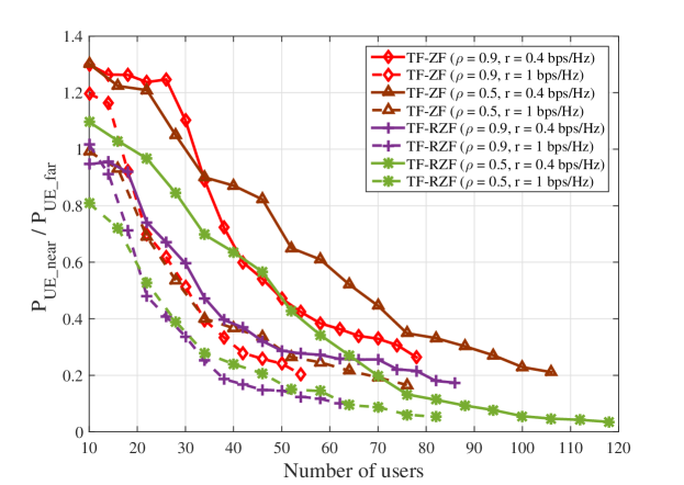
Figure 16: The total transmit power for near UEs and far UEs ratio vs. the number of users.

Fig. 15 and Fig. 16 plot the time-fraction ratio and power ratio, which are different from their counter parts in the above considered single-cell and two-cell cases. The number of near UEs during the time-fraction $\tau$ is half of that during the time-fraction $1-\tau$ but the number of cell-edge UEs during the former fraction is double to that during the latter fraction. This fact dictates the allocation for both time-fractions and powers.

V Conclusions

We have considered the problem of maximizing the energy efficiency in assuring the QoS for large numbers of users by multi-cell massive MIMO beamforming. The antennas’ spatial correlation, which is an important factor in assessing the actual capacity of massive MIMO, has been incorporated in our consideration. To serve even larger numbers of users within a time slot, techniques of time-fraction-wise beamforming have been proposed, including new path-following computational procedures for computational solution. The provided simulations have demonstrated that $8$ $\times$ $8$ antenna array equipped massive MIMO is able to serve up to $160$ users at required QoSs.

Appendix: fundamental inequalities

By noting that function $f(x,y,t)=\frac{\ln(1+1/xy)}{t}$ is convex in $x>0,y>0,t>0$ [30], the following inequality for all $x>0$, $\bar{x}>0$, $y>0$, $\bar{y}>0$, $t>0$, $\bar{t}>0$ holds true [31]:

$$\displaystyle\frac{\ln(1+1/xy)}{t} \geq f(\bar{x},\bar{y},\bar{t})+\langle\nabla f(\bar{x},\bar{y},\bar{t}),(x,y,t)-(\bar{x},\bar{y},\bar{t})\rangle$$ (71)

$$= \bar{a}-\bar{b}x-\bar{c}y-\bar{d}t,$$

and

$$\displaystyle\ln(1+1/xy) \geq a-bx-cy,$$ (72)

where $\nabla$ is the gradient operation and

$$\begin{array}[]{c}\bar{a}=2\displaystyle\frac{\ln(1+1/\bar{x}\bar{y})}{\bar{t}}+\frac{2}{\bar{t}(\bar{x}\bar{y}+1)}>0,\bar{b}=\frac{1}{(\bar{x}\bar{y}+1)\bar{x}\bar{t}}>0,\\ \bar{c}=\displaystyle\frac{1}{(\bar{x}\bar{y}+1)\bar{y}\bar{t}}>0,\bar{d}=\frac{\ln(1+1/\bar{x}\bar{y})}{\bar{t}^{2}}>0,\end{array}$$

and

$$a=\ln(1+1/\bar{x}\bar{y})+2/(\bar{x}\bar{y}+1)>0,b=1/(\bar{x}\bar{y}+1)\bar{x}>0,c=1/(\bar{x}\bar{y}+1)\bar{y}>0.$$

Replacing $x\rightarrow 1/x$ and $\bar{x}\rightarrow 1/\bar{x}$ in (72) leads to another inequality

$$\displaystyle\ln(1+x/y) \geq \tilde{a}-\tilde{b}/x-\tilde{c}y,$$ (73)

for

$$\tilde{a}=\ln(1+\bar{x}/\bar{y})+2\bar{x}/(\bar{x}+\bar{y})>0,\tilde{b}=\bar{x}^{2}/(\bar{x}+\bar{y})>0,\tilde{c}=\bar{x}/(\bar{x}+\bar{y})\bar{y}>0.$$

Observing that function $f(z,t)={1}/{zt}$ is convex in $z>0,t>0$, we also have the following inequality

$$\frac{1}{zt} \geq f(\bar{z},\bar{t})+\langle\nabla f(\bar{z},\bar{t}),(z,t)-(\bar{z},\bar{t})\rangle$$ (74)

$$= 3\frac{1}{\bar{z}\bar{t}}-\left(\frac{z/\bar{z}+t/\bar{t}}{\bar{z}\bar{t}}\right),\quad\forall\ x>0,\ \bar{x}>0,t>0,\bar{t}>0.$$

References

• [1] F. Rusek et al, “Scaling up MIMO: opportunities and challenges with very large arrays,” IEEE Signal Process. Mag., vol. 30, no. 1, pp. 40–60, Jan 2013.
• [2] E. G. Larsson, O. Edfors, F. Tufvesson, and T. L. Marzetta, “Massive MIMO for next generation wireless systems,” IEEE Commun. Mag., vol. 52, no. 2, pp. 186–195, February 2014.
• [3] T. L. Marzetta, “Noncooperative cellular wireless with unlimited numbers of base station antennas,” IEEE Trans. Wireless Commun., vol. 9, no. 11, pp. 3590–3600, Nov. 2010.
• [4] H. Q. Ngo, E. G. Larsson, and T. L. Marzetta, “Aspects of favorable propagation in massive MIMO,” in 22nd European Signal Process. Conf. (EUSIPCO), Lisbon, Portugal, 2014, pp. 76–80.
• [5] A. M. Tulino and S. Verdu, Random Matrix Theory and Wireless Communications.   Delft, The Netherlands: Now Publishers Inc., 2004.
• [6] R. Couillet and M. Debbah, Random Matrix Methods for Wireless Communications,.   Cambridge, U.K.: Cambridge Univ. Press, 2011.
• [7] S. Wagner, R. Couillet, M. Debbah, and D. T. M. Slock, “Large system analysis of linear precoding in correlated MISO broadcast channels under limited feedback,” IEEE Trans. Inf. Theory, vol. 58, no. 7, pp. 4509–4537, Jul. 2012.
• [8] H. Yang and T. L. Marzetta, “Performance of conjugate and zero-forcing beamforming in large-scale antenna systems,” IEEE J. Selected Areas in Commun., vol. 31, no. 2, pp. 172–179, Feb. 2013.
• [9] Y. G. Lim, C. B. Chae, and G. Caire, “Performance analysis of massive MIMO for cell-boundary users,” IEEE Trans. Wireless Commun., vol. 14, no. 12, pp. 6827–6842, Dec 2015.
• [10] L. D. Nguyen, H. D. Tuan, T. Q. Duong, and H. V. Poor, “Beamforming and power allocation for energy-efficient massive MIMO,” in Proc. 22nd Inter. Conf. Digital Signal Process. (DSP2017), Aug. 2017, p. 105.
• [11] C. B. Peel, B. M. Hochwald, and A. L. Swindlerhurst, “A vector-perturbation technique for near capacity multiantenna multiuser communication-part i: channel inversion and regularization,” IEEE Trans. Commun., vol. 53, no. 1, pp. 195–202, Jan. 2005.
• [12] H. Q. Ngo, E. G. Larsson, and T. L. Marzetta, “Energy and spectral efficiency of very large multiuser MIMO systems,” IEEE Trans. Commun., vol. 61, no. 4, pp. 1436–1449, April 2013.
• [13] D.-S. Shiu, G. J. Foschini, M. J. Gans, and J. M. Kahn, “Fading correlation and its effect on the capacity of multielement antenna systems,” IEEE Trans. Commun., vol. 48, no. 3, pp. 502–513, Mar. 2000.
• [14] A. Adhikary, J. Nam, J. Y. Ahn, and G. Caire, “Joint spatial division and multiplexing - the large-scale array regime,” IEEE Trans. Inf. Theory, vol. 59, no. 10, pp. 6441–6463, Oct 2013.
• [15] S. Buzzi, C.-L. I, T. E. Klein, H. V. Poor, C. Yang, and A. Zappone, “A survey of energy-efficient techniques for 5G networks and challenges ahead,” IEEE J. Select. Areas Commun., vol. 34, no. 4, pp. 697–709, Apr. 2016.
• [16] A. Zappone, L. Sanguinetti, G. Bacci, E. A. Jorswieck, and M. Debbah, “Energy-efficient power control: A look at 5G wireless technologies,” IEEE Trans. Signal Process., vol. 64, no. 7, pp. 1668–1683, Apr. 2016.
• [17] T. Yoo and A. Goldsmith, “On the optimality of multiantenna broadcast scheduling using zero-forcing beamforming,” IEEE J. Sel. Areas Commun., vol. 54, no. 3, pp. 528–541, Mar. 2006.
• [18] A. Adhikary, H. S. Dhillon, and G. Caire, “Massive-mimo meets hetnet: Interference coordination through spatial blanking,” IEEE J. Sel. Areas Commun., vol. 33, no. 6, pp. 1171–1186, June 2015.
• [19] Z. Sheng, H. D. Tuan, H. H. Nguyen, and M. Debbah, “Optimal training sequences for large-scale MIMO-OFDM systems,” IEEE Trans. Signal Process., vol. 65, no. 13, pp. 3329–3343, Jul. 2017.
• [20] Z. Sheng, H. D. Tuan, H. H. M. Tam, H. H. Nguyen, and Y. Fang, “Energy-efficient precoding in multicell networks with full-duplex base stations,” EURASIP J. Wirel. Commun. Networking, 2017, DOI 10.1186/s13638-017-0831-5.
• [21] Z. Sheng, H. D. Tuan, T. Q. Duong, and H. V. Poor, “Joint power allocation and beamforming for energy-efficient two-way multi-relay communications,” IEEE Trans. Wirel. Commun., vol. PP, no. 99, pp. 1–1, 2017.
• [22] V.-D. Nguyen, T. Q. Duong, H. D. Tuan, O.-S. Shin, and H. V. Poor, “Spectral and energy efficiencies in full-duplex wireless information and power transfer,” IEEE Trans. Commun., vol. 65, no. 5, pp. 2220–2232, May 2017.
• [23] B. R. Marks and G. P. Wright, “A general inner approximation algorithm for nonconvex mathematical programs,” Operation Research, vol. 26, no. 4, pp. 681–683, 1978.
• [24] V. K. Nguyen and J. S. Evans, “Multiuser transmit beamforming via regularized channel inversion: a large system analysis,” in Proc. of 2008 Conf. Global Commun. (Globecom), 2008, pp. 1–4.
• [25] Z. Wang and W. Chen, “Regularized zero-forcing for multiantenna broadcast channels with user selection,” IEEE Wireless Commun. Lett., vol. 1, no. 2, pp. 129–132, April 2012.
• [26] Y. Kim et al, “Full-dimension MIMO (FD-MIMO): The next evolution of MIMO in LTE systems,” IEEE Wireless Commun., vol. 21, no. June, pp. 26–33, 2014.
• [27] S. Wagner, R. Couillet, M. Debbah, and D. T. M. Slock, “Large system analysis of linear precoding in correlated miso broadcast channels under limited feedback,” IEEE Trans. Inf. Theory, vol. 58, no. 7, pp. 4509–4537, July 2012.
• [28] E. Bjornson, M. Kountouris, and M. Debbah, “Massive MIMO and small cells: improving energy efficiency by optimal soft-cell coordination,” in ICT, May 2013, pp. 1–5.
• [29] J. G. Andrews, S. Buzzi, W. Choi, S. V. Hanly, A. Lozano, A. C. K. Soong, and J. C. Zhang, “What will 5G be?” IEEE J. Sel. Areas Commun., vol. 32, no. 6, pp. 1065–1082, June 2014.
• [30] Z. Sheng, H. D. Tuan, A. A. Nasir, T. Q. Duong, and H. V. Poor, “Power allocation for energy efficiency and secrecy of interference wireless networks,” [Online]. Available:http://arxiv.org/abs/1708.07334.
• [31] H. Tuy, Convex Analysis and Global Optimization (second edition).   Springer International, 2017.