Peephole: Predicting Network Performance Before Training
Abstract
The quest for performant networks has been a significant force that drives the advancements of deep learning in recent years. While rewarding, improving network design has never been an easy journey. The large design space combined with the tremendous cost required for network training poses a major obstacle to this endeavor. In this work, we propose a new approach to this problem, namely, predicting the performance of a network before training, based on its architecture. Specifically, we develop a unified way to encode individual layers into vectors and bring them together to form an integrated description via LSTM. Taking advantage of the recurrent network’s strong expressive power, this method can reliably predict the performances of various network architectures. Our empirical studies showed that it not only achieved accurate predictions but also produced consistent rankings across datasets – a key desideratum in performance prediction.
1 Introduction
The computer vision community has witnessed a series of breakthroughs over the past several years. What lies behind this remarkable progress is the advancement in Convolutional Neural Networks (CNNs) [14, 13]. From AlexNet [13], VGG [21], GoogLeNet [23], to ResNet [7], we have come a long way in improving the network design, which also results in substantial performance improvement. Take ILSVRC [4] for example, the classification error rate has dropped from to below in just a few years, primarily thanks to the evolution of network architectures. Nowadays, “using a better network” has become a commonly adopted strategy to boost performance – this strategy, while simple, has been repeatedly shown to be very effective in practical applications, e.g. recognition [4], detection [17], and segmentation [6].
However, improving network designs is non-trivial. Along this way, we are facing two key challenges, namely, the large design space and the costly training process. Specifically, to devise a convolutional network, one has to make a number of modeling choices, e.g. the number of layers, the number of channels within these layers, and whether to insert a pooling layer at certain points, etc. All such choices together constitute a huge design space that is simply beyond our means to conduct a thorough investigation. Previous efforts were mostly motivated by intuitions – though fruitful in early days, this approach has met increasing difficulties as networks become more complicated.
In recent works [27, 1, 28, 26], automatic search methods have been proposed. These methods seek better designs (within a restricted design space), by gradually adjusting parts of the networks and validating the generated designs on real datasets. Without an effective prior guidance, such search procedures tend to spend lots of resources in evaluating “unpromising” options. Also note that training a network in itself is a time-consuming process. Even on a dataset of moderate size, it may take hours (if not days) to train a network. Consequently, an excessively long process is generally needed to to find a positive adjustment. It’s been reported [27, 28] that searching a network on CIFAR takes hundreds of GPUs for a lengthy period.
Like many others in this community, we have our own share of painful experience in finding good network designs. To mitigate this lengthy and costly process, we develop an approach to quantitatively assess an architecture before investing resources in training it. More accurately, we propose a model, called Peephole, to predict the final performance of an architecture before training.
In this work, we explore a natural idea, that is, to formulate the network performance predictor as a regression model, which accepts a network architecture as the input and produces a score as a predictive estimate of its performance, e.g. the accuracy on the validation set. Here, the foremost question is how to turn a network architecture into a numerical representation. This is nontrivial given the diversity of possible architectures. We tackle this problem in two stages. First, we develop a vector representation, called Unified Layer Code, to encode individual layers. This scheme allows various layers to be represented uniformly and effectively by vectors of a fixed dimension. Second, we introduce an LSTM network to integrate the layer representations, which allows architectures with different depths and topologies to be handled in a uniform way.
Another challenge that we face is how to obtain a training set. Note that this task differs essentially from conventional ones in that the samples are network architectures together with their performances instead of typical data samples like images or data records. Here, the sample space is huge and it is very expensive to obtain even a sample (which involves running an entire training procedure). In addressing this issue, we draw inspirations from engineering practice, and develop a block-based sampling scheme, which generates new architectures by integrating the blocks sampled from a Markov process. This allows us to explore a large design space with limited budget while ensuring that each sample architecture is reasonable.
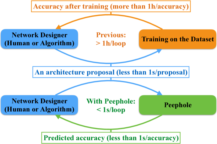
Overall, our main contributions lie in three aspects: (1) We develop Peephole, a new framework for predicting network performance based on Unified Layer Code and Layer Embedding. Our Peephole can predict a network’s performance before training. (2) We develop Block-based Generation, a simple yet effective strategy to generate a diverse set of reasonable network architectures. This allows the proposed performance predictor to be learned with an affordable budget. (3) We conducted empirical studies over more than a thousand networks, which show that the proposed framework can make reliable predictions for a wide range of network architectures and produce consistent ranking across datasets. Hence, its predictions can provide an effective way to search better network designs, as shown in Figure 1.
2 Related Work
Network Design.
Since the debut of AlexNet [13], CNNs have become widely adopted to solve computer vision problems. Over the past several years, the advances in network design have been a crucial driving force behind the progress in computer vision. Many representative architectures, such as AlexNet [13], VGGNet [21], GoogLeNet [23], ResNet [7], DenseNet [9], and DPN [3] are designed manually, based on intuitions and experience. Nonetheless, this approach has become less rewarding. The huge design space combined with the costly training procedure makes it increasingly difficult to obtain an improved design.
Recently, the community has become more interested in an alternative approach, namely automatic network design. Several methods [27, 1, 28, 26] have been proposed. These methods rely on reinforcement learning to learn how to improve a network design. In order to supervise the learning process, all these methods rely on actual training processes to provide feedback, which are very costly, in both time and computational resources. Our work differs essentially. Instead of developing an automatic design technique, we focus on a crucial but often overlooked problem, that is, how to quickly get the performance feedback.
Network Performance Prediction.
As mentioned, our approach is to predict network performance. This is an emerging topic, on which existing works remain limited. Some previous methods on performance prediction were developed in the context of hyperparameter optimization, using techniques like Gaussian Process [22] or Last-Seen-Value heuristics [16]. These works mainly focus on designing a special surrogate function for a better evaluation of hyper-configurations. There have also been attempts to directly predict network performance. Most works along this line intend to extrapolate the future part of the learning curve given the elapsed part. For this, Domhan et al. [5] proposed a mixture of parametric functions to model the learning curve. Klein et al. [11] extended this work by replacing the mixture of functions with a Bayesian Neural Network. Baker et al. [2] furthered this study by additionally leveraging the information about network architectures with hand-crafted features, and using -SVR for curve prediction.
All these works rely on partially observed learning curves to make predictions, which still involve a partly run training procedure and therefore are time-consuming. To support large-scale search of network designs, we desire much quicker feedback and thus explore a fundamentally different but more challenging approach, that is, to predict the performance purely based on architectures.

3 Network Performance Prediction
Our goal is to develop an effective method to predict network performance before training. Our predictive model, called Peephole and shown in Figure 2, can be formalized as a function, denoted by . The function takes two arguments, a network architecture and an epoch index , and produces a scalar value as the prediction of the accuracy at the end of the -th epoch. Here, incorporating the epoch index as an input to is reasonable, as the validation accuracy generally changes as the training proceeds. Therefore, when we predict performance, we have to be specific about the time point of the prediction.
Note that this formulation differs fundamentally from previous works [5, 11, 2]. Such methods require the observation of the initial part (usually ) of the training curve and extrapolate the remaining part. On the contrary, our method aims to predict the entire curve, relying only on the network architecture. In this way, it can provide feedback much quicker and thus is particularly suited for large-scale search of network designs.
However, developing such a predictor is nontrivial. Towards this goal, we are facing significant technical challenges, e.g. how to unify the representation of various layers, and how to integrate the information from individual layers over various network topologies. In what follows, we will present our answers to these questions. Particularly, Sec. 3.1 presents a unified vector representation of layers, which is constructed in two steps, namely coding and embedding. Sec. 3.2 presents an LSTM model for integrating the information across layers.
3.1 Unified Layer Code
| Layer | TY | KW | KH | CH |
|---|---|---|---|---|
| Conv | ||||
| Max-Pool | ||||
| Avg-Pool | ||||
| ReLU | ||||
| Sigmoid | ||||
| Tanh | ||||
| BN |
In general, a convolutional neural network can be considered as a directed graph whose nodes represent certain operations, e.g. convolution and pooling. Hence, to develop a representation of such a graph, the first step is to define a representation of individual nodes, i.e. the layers. In this paper, we propose Unified Layer Code (ULC), a uniform scheme to encode various layers into numerical vectors, which is done in two steps: integer coding and embedding.
Integer coding.
We notice that the operations commonly used in a CNN, including convolution, pooling, and nonlinear activation, can all be considered as applying a kernel to the input feature map. To produce an output value, the kernel takes a local part of the feature map as input, applies a linear or nonlinear transform, and then yields an output. In particular, an element-wise activation function can be considered as a nonlinear kernel of size .
Each operation is also characterized by the number of output channels. In a typical CNN, the number of channels can vary significantly, from below to thousands. However, for a specific layer, this number is usually decided based on that of the input, according to a ratio within a limited range. Particularly, for both pooling and nonlinear activation, the numbers of output channels are always equal to that of the input channels, and thus the ratio is . While for convolution, the ratio usually ranges from to , depending on whether the operation intends to reduce, preserve, or expand the representation dimension. In light of this, we choose to represent CH by the output-input ratio instead of the absolute number. In this way, we can effectively limit its dynamic range, quantize it into bins (respectively centered at ).
Overall, we can represent a common operation by a tuple of four integers in the form of (TY, KW, KH, CH), where TY is an integer id that indicates the type of the computation, KW and KH are respectively the width and height of the kernel, while CH represents the ratio of output-input channels (using the the index of the quantized bin). The details of this scheme are summarized in Table 1.
Layer embedding.
While capturing the key information for a layer, the discrete representation introduced above is not amenable to complex numerical computation and deep pattern recognition. Inspired by word embedding [20], a strategy proven to be very effective in natural language processing, we take one step further and develop Layer Embedding, a scheme to turn the integer codes into a unified real-vector representation.
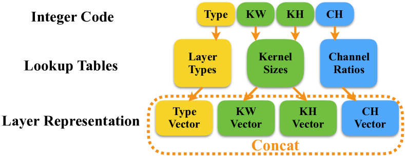
As shown in Figure 3, the embedding is done by table lookup. Specifically, this module is associated with three lookup tables, respectively for layer types, kernel sizes, and channel ratios. Note that the kernel size table is used to encode both KW and KH. Given a tuple of integers, we can convert its element into a real vector by retrieving from the corresponding lookup table. Then by concatenating all the embedded vectors derived respectively from individual integers, we can form a vector representation of the layer.
3.2 Integrated Prediction
With the layer-wise representations based on Unified Layer Code and Layer Embedding, the next is to aggregate them into an overall representation for the entire network. In this work, we focus on the networks with sequential structures, which already constitute a significant portion of the networks used in real-world practice. Here, the challenge is how to cope with varying depths in a uniform way.
Inspired by the success of recurrent networks in sequential modeling, e.g. in language modeling [19] and video analytics [25], we choose to explore recurrent networks in our problem. Specifically, we adopt the Long-Short Term Memory (LSTM) [8], an effective variant of RNN, for integrating the information along a sequence of layers. In particular, an LSTM network is composed of a series of LSTM units, each for a time step (i.e. a layer in our context). The LSTM maintains a hidden state and a cell memory , and uses an input gate , an output gate , and a forget gate to control the information flow. At each step, it takes an input , decides the value of all the gates, yields an output , and updates both the hidden state and the cell memory , as follows:
| (1) |
Here, denotes the sigmoid function while the element-wise product. Along the way from low-level to high-level layers, the LSTM network would gradually incorporate layer-wise information into the hidden state. At the last step, i.e. the layer right before the fully connected layer for classification, we extract the hidden state of the LSTM cell to represent the overall structure of the network, which we refer to as the structural feature.
As shown in Figure 2, the Peephole framework will finally combine this structural feature with the epoch index (also embedded into a real-vector) and use a Multi-Layer Perceptron (MLP) to make the final prediction of accuracy. In particular, the MLP component at the final step is comprised of three fully connected layers with Batch Normalization and ReLU activation. The output of this component is a real value that serves as an estimate of the accuracy.
4 Training Peephole
Like other predictive models, Peephole requires sufficient training samples to learn its parameters. However, for our problem, the preparation of the training set itself is a challenge. Randomly sampling sequences of layers is not a viable solution for two reasons: (1) The design space grows exponentially as the number of layers increases, while it is expensive to obtain a training sample (which requires running an entire training procedure to obtain a performance curve). Hence, it is unaffordable to explore the entire design space freely, even with a large amount of computational resources. (2) Many combinations of layers are not reasonable options from a practical point of view (e.g. a network with multiple activation layers stacked consecutively in a certain part of the layer sequence). Training such networks are simply a waste of resources.
In this section, we draw inspirations from existing practice and propose a Block-based Generation scheme to acquire training samples in Sec. 4.1. Then, we present a learning objective for supervising the training process in Sec. 4.2.
4.1 Block-based Generation
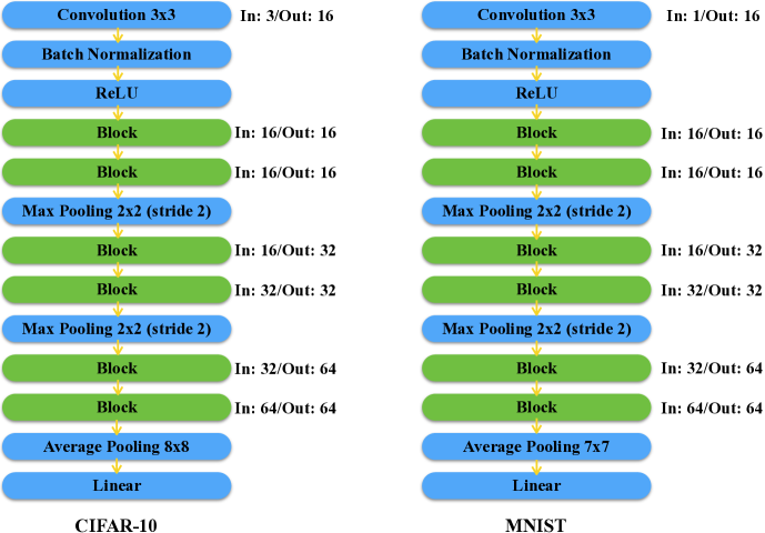
The engineering practice of network design [7, 24] suggests that it is a good strategy to construct a neural network by stacking blocks that are structurally alike. Zoph et al. [28] and Zhong et al. [26] also proposed to search transferable blocks (referred to as cells in [28]) and assemble them into a network in their efforts towards an automatic way for network search. Inspired by these works, we propose Block-based Generation, a simple yet effective strategy to prepare our training samples. As illustrated in Figure 3, it first designs individual blocks and then stacks them into a network following a certain skeleton.
A block is defined to be a short sequence of layers with no more than layers. To generate a block, we follow a Markov chain. Specifically, we begin with a convolution layer by randomly choosing its kernel size from and the ratio of output/input channel numbers from . Then at each step, we draw the next layer conditioned on the current one following predefined transition probabilities between layer types, which are empirically estimated from practical networks. For example, a convolution layer has a high chance to be followed by a batch normalization layer and a nonlinear activation. An activation layer is more likely to ensued by another convolution layer or a pooling layer. More details will be provided in the supplemental materials.
With a collection of blocks, we can then build a complete network by assembling them following a skeleton. The design of the skeleton follows the general practice in computer vision. As shown in Figure 4, the skeleton comprises three stages with different resolutions. Each stage is a stack of blocks followed by a max pooling layer to reduce the spatial resolution. The features from the last block will go through an average pooling layer and then a linear layer for classification. When replicating blocks within a stage, convolution layers will be inserted in between for dimension adaptation when the output dimension of the preceding layer does not match the input dimension of the next layer.
The block-based generation scheme presented above effectively constrain the sample space, ensuring that the generated networks are mostly reasonable and making it feasible to prepare a training set with an affordable budget.
4.2 Learning Objective
Given a set of sample networks , we can obtain a performance curves for each network , i.e. the validation accuracy as a function of epoch numbers, by training the network on a given dataset. Hence, we can obtain a set of pairs and learn the parameters of the predictor in a supervised way.
Specifically, we formulate the learning objective with the smooth L1 loss, denoted by , as below:
| (2) |
Here, denotes the predictor parameters. Note that we train each sample network with epochs, and use the results of the final epoch to supervise the learning process. Our framework is very flexible – with the entire learning curves, in principle, one can use the results at multiple epochs for training. However, we found empirically that using only the final epochs already yields reasonably good results.
4.3 Discussions
First, the Peephole predictor is task-specific. It is trained to predict the performance on a certain dataset with a specific performance metric. Second, besides network architectures and epoch numbers, the performance of a network also depends on a number of other factors, e.g. how it is initialized, how the learning rate is adjusted over time, as well as the settings on the optimizers. In this work, we train all sample networks with a fixed set of or such design choices.
Admittedly, such a setting may sound a bit restrictive. However, this actually reflects our typical practice when tuning network designs in ablation studies. Moreover, most automatic network search schemes also fix such choices during the search process in order to fairly compare among architectures. Therefore, the predictor trained in this way can already provide good support to the practice. That being said, we do plan to incorporate additional factors in the predictor in our future exploration.
5 Experiments
We tested Peephole, the proposed network performance prediction framework on two public datasets, CIFAR-10 [12] and MNIST [15]. Sec. 5.1 presents the experiment settings, including how the datasets are used and the implementation details of our framework. Sec. 5.2 presents the results we obtained on both datasets, and compares them with other performance prediction methods. Sec. 5.3 presents preliminary results on using Peephole to guide the search of better networks on ImageNet. Finally, Sec. 5.4 presents a qualitative study on the learned representations via visualization.
| CIFAR-10 | MNIST | |||
|---|---|---|---|---|
| Train | Validation | Train | Validation | |
| Size | ||||
| Mean | ||||
| Std | ||||
| Min | ||||
| Max | ||||
5.1 Experiment Configurations
Datasets.
CIFAR-10 [12] is a dataset for object classification. In recent years, it usually serves as the testbed for convolutional network designs. MNIST [15] is a dataset for hand-written digit classification, one of the early and widely used datasets for neural network research. Both datasets are of moderate scale. We chose them as the basis for our study because it is affordable for us to train over a thousand networks thereon to investigate the effectiveness of the proposed predictor. After all, our goal is to explore an performance prediction method that works with diverse architectures instead of pursing a state-of-the-art network on large-scale vision benchmarks. To prepare the samples for training and validation, we follow the procedure described in Sec. 4 to generate two sets of networks, respectively for CIFAR-10 and MNIST, and train them to obtain performance curves.
Detailed settings.
For fair comparison, we train all sampled networks with the same setting: We use SGD with momentum and weight decay . Each epoch loops over the entire training set in random order. The learning rate is initialized to and scaled down by a factor of every epochs (for CIFAR-10) or epochs (for MNIST). The network weights are all initialized following the scheme in [7]. Table 2 shows the statistics of these networks and their performances.
For the Peephole model, we use -dimensional vectors for both layer embedding and epoch embedding. The dimension of the hidden states in LSTM is set to . The Multi-Layer Perceptron (MLP) for final prediction comprises linear layers, each with hidden units.
5.2 Comparison of Prediction Accuracies
Methods to compare.
We compare our Peephole method with two representative methods in recent works:
-
1.
Bayesian Neural Network (BNN) [11]. This method is devised to extrapolate learning curves given their initial portions (usually of the entire ones). It represents each curve as a linear combination of basis functions and uses Bayesian Neural Network to yield probabilistic extrapolations.
-
2.
-Support Vector Regression (-SVR) [2]. This method relies on a regression model, -SVR, to make predictions. To predict the performance of a network this model takes as input both the initial portion of the learning curve and simple heuristic features derived based on the network architecture. This method represents the state of the art on this task.
Note that both methods above require the initial portions of the learning curves while ours can give feedback purely based on the network architecture before training.
Evalution criteria.
We evaluate the predictor performances using three criteria:
-
1.
Mean Square Error (MSE), which directly measures the deviation of the predictions from the actual values.
-
2.
Kendall’s Tau (Tau), which measures the correlation between the predictive rankings among all testing networks and their actual rankings. The value of Kendall’s Tau ranges from to , and a higher value indicates higher correlation.
-
3.
Coefficient of Determination (), which measures how closely the predicted value depends on the actual value. The value of ranges from to , where a value closer to suggests that the prediction is more closely coupled with the actual value.
| Method | MSE | Tau | |
|---|---|---|---|
| BNN | |||
| -SVR | |||
| Peephole (Ours) |
| Method | MSE | Tau | |
|---|---|---|---|
| BNN | |||
| -SVR | |||
| Peephole (Ours) |
Results on CIFAR-10.
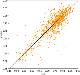
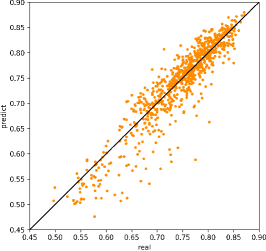
Table 3 compares the prediction results for the networks trained on CIFAR-10, obtained with different predictors. We observe that Peephole consistently outperforms both BNN and -SVR across all metrics. Particularly, achieving smaller MSE means that the predictions from Peephole are generally more accurate than those from others. This makes it a viable predictor in practice. On the other hand, the high values in Tau and indicate that the ranking among multiple networks produced by Peephole is quite consistent with the ranking of their actual performances. This makes Peephole a good criterion to select performant network architectures.
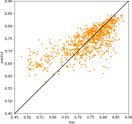
The scatter plots in Figure 5 visualize the correlations between the predicted accuracies and actual accuracies, obtained with different methods. Qualitatively, the predictions made by Peephole demonstrate notably higher correlation with the actual values than those from other methods, especially at the high-accuracy area (top right corner).
Results on MNIST.
We also evaluated the predictions on the networks trained on MNIST in the same way, with the results shown in Table 4. Note that since most networks can yield high accuracies on this MNIST, it would be easier to produce more precise predictions on the accuracy numbers but more difficult to yield consistent rankings. This is reflected by the performance metrics in the table. Despite this difference in data characteristics, Peephole still significantly outperforms the other two methods across all metrics.
| Model | #Param | CIFAR-10 | ImageNet | ||
|---|---|---|---|---|---|
| Pred | Real | Top-1 | Top5 | ||
| VGG-13 | M | – | – | ||
| Selected | M | ||||
5.3 Transfer to ImageNet
Getting top performance on ImageNet is a holy grail for convolutional network design. Yet, directly training Peephole based on ImageNet is prohibitively expensively due to the lengthy processes of training a network on ImageNet. Nevertheless, [28] suggests an alternative way, that is, to search for scalable and transferable block architectures on a smaller dataset like CIFAR-10. Following this idea, we select the network architecture with the highest Peephole-predicted accuracy among those in our validation set for CIFAR-10, then scale it up and transfer it to ImageNet111The details of the selected network and this transfer process will be provided in the supplemental materials..
We compared this network with VGG-13 [21], a widely used network that was designed manually. From the results in Table 5, we can see that the selected network achieves moderately better accuracy on ImageNet with a substantially smaller parameter size. This is just a preliminary study. But it shows that Peephole is promising for pursuing performant network designs that are transferable to the larger datasets.
5.4 Studies on the Representations
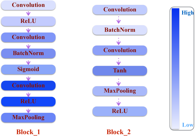
The effective of Peephole may be attributed to its ability to abstract a uniform but expressive representation for various architectures. To gain better understanding of this representation, we analyze the learned LSTM and the derived feature vectors.
In one study, we examined the hidden cells inside the LSTM using the method presented in [10]. Particularly, we recorded the dynamics of the cell responses as the LSTM traverses the sequence of layers. Figure 6 shows the responses of a certain cell, where we can see that the response raises every time it gets to a convolution layer. This behavior is observed in different blocks. This observation suggests that this cell learns to “detect” convolution layers even without being explicitly directed to do. In a certain sense, this also reflects the capability of LSTM to capture architectural patterns.
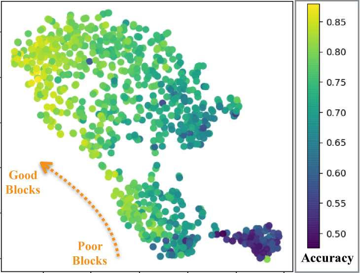
In another study, we visualized the structural feature (derived from the last unit of the LSTM) using t-SNE embedding [18]. Figure 7 shows the visualized results. We can see the gradual transition from low performance networks to high performance networks. This shows that the structural features contain key information related to the network performances.
6 Conclusion
We presented Peephole, a predictive model for predicting network performance based on architectures before training. Specifically, we developed Unified Layer Code as a unified representation for network architectures and a LSTM-based model to integrate the information from individual layers. To tackle the difficulties in preparing the training set, we propose a Block-based Generation scheme, which allows us to explore a wide variety of reasonable designs while constraining the search space. The systematic studies with over a thousand networks trained on CIFAR-10 and MNIST showed that the proposed method can yield reliable predictions that are highly correlated with the actual performance. On three different metrics, our method significantly outperforms previous methods.
We note that this is just the first step towards the goal of fast search of network designs. In future work, we plan to incorporate additional factors in our predictor, such as various design choices, to extend the applicability of the predictive model. We will also explore more effective ways to optimize network designs on top of this predictive model.
References
- [1] B. Baker, O. Gupta, N. Naik, and R. Raskar. Designing neural network architectures using reinforcement learning. CoRR, abs/1611.02167, 2016.
- [2] B. Baker, O. Gupta, R. Raskar, and N. Naik. Practical neural network performance prediction for early stopping. arXiv preprint arXiv:1705.10823, 2017.
- [3] Y. Chen, J. Li, H. Xiao, X. Jin, S. Yan, and J. Feng. Dual path networks. arXiv preprint arXiv:1707.01629, 2017.
- [4] J. Deng, W. Dong, R. Socher, L.-J. Li, K. Li, and L. Fei-Fei. Imagenet: A large-scale hierarchical image database. In Computer Vision and Pattern Recognition, 2009. CVPR 2009. IEEE Conference on, pages 248–255. IEEE, 2009.
- [5] T. Domhan, J. T. Springenberg, and F. Hutter. Speeding up automatic hyperparameter optimization of deep neural networks by extrapolation of learning curves. In Twenty-Fourth International Joint Conference on Artificial Intelligence, 2015.
- [6] M. Everingham, L. Van Gool, C. K. Williams, J. Winn, and A. Zisserman. The pascal visual object classes (voc) challenge. International journal of computer vision, 88(2):303–338, 2010.
- [7] K. He, X. Zhang, S. Ren, and J. Sun. Deep residual learning for image recognition. In Proceedings of the IEEE Conference on Computer Vision and Pattern Recognition, pages 770–778, 2016.
- [8] S. Hochreiter and J. Schmidhuber. Long short-term memory. Neural computation, 9(8):1735–1780, 1997.
- [9] G. Huang, Z. Liu, K. Q. Weinberger, and L. van der Maaten. Densely connected convolutional networks. arXiv preprint arXiv:1608.06993, 2016.
- [10] A. Karpathy, J. Johnson, and L. Fei-Fei. Visualizing and understanding recurrent networks. arXiv preprint arXiv:1506.02078, 2015.
- [11] A. Klein, S. Falkner, J. T. Springenberg, and F. Hutter. Learning curve prediction with bayesian neural networks. International Conference on Learning Representations, 2017.
- [12] A. Krizhevsky, V. Nair, and G. Hinton. Cifar-10 and cifar-100 datasets. URl: https://www. cs. toronto. edu/~ kriz/cifar.html, 2009.
- [13] A. Krizhevsky, I. Sutskever, and G. E. Hinton. Imagenet classification with deep convolutional neural networks. In Advances in neural information processing systems, pages 1097–1105, 2012.
- [14] Y. LeCun, L. Bottou, Y. Bengio, and P. Haffner. Gradient-based learning applied to document recognition. Proceedings of the IEEE, 86(11):2278–2324, 1998.
- [15] Y. LeCun, C. Cortes, and C. J. Burges. The mnist database of handwritten digits, 1998.
- [16] L. Li, K. Jamieson, G. DeSalvo, A. Rostamizadeh, and A. Talwalkar. Hyperband: A novel bandit-based approach to hyperparameter optimization. arXiv preprint arXiv:1603.06560, 2016.
- [17] T.-Y. Lin, M. Maire, S. Belongie, J. Hays, P. Perona, D. Ramanan, P. Dollár, and C. L. Zitnick. Microsoft coco: Common objects in context. In European Conference on Computer Vision, pages 740–755. Springer, 2014.
- [18] L. v. d. Maaten and G. Hinton. Visualizing data using t-sne. Journal of Machine Learning Research, 9(Nov):2579–2605, 2008.
- [19] T. Mikolov, M. Karafiát, L. Burget, J. Černockỳ, and S. Khudanpur. Recurrent neural network based language model. In Eleventh Annual Conference of the International Speech Communication Association, 2010.
- [20] T. Mikolov, I. Sutskever, K. Chen, G. S. Corrado, and J. Dean. Distributed representations of words and phrases and their compositionality. In Advances in neural information processing systems, pages 3111–3119, 2013.
- [21] K. Simonyan and A. Zisserman. Very deep convolutional networks for large-scale image recognition. arXiv preprint arXiv:1409.1556, 2014.
- [22] K. Swersky, J. Snoek, and R. P. Adams. Freeze-thaw bayesian optimization. arXiv preprint arXiv:1406.3896, 2014.
- [23] C. Szegedy, W. Liu, Y. Jia, P. Sermanet, S. Reed, D. Anguelov, D. Erhan, V. Vanhoucke, and A. Rabinovich. Going deeper with convolutions. In Proceedings of the IEEE Conference on Computer Vision and Pattern Recognition, pages 1–9, 2015.
- [24] S. Xie, R. Girshick, P. Dollár, Z. Tu, and K. He. Aggregated residual transformations for deep neural networks. arXiv preprint arXiv:1611.05431, 2016.
- [25] J. Yue-Hei Ng, M. Hausknecht, S. Vijayanarasimhan, O. Vinyals, R. Monga, and G. Toderici. Beyond short snippets: Deep networks for video classification. In Proceedings of the IEEE conference on computer vision and pattern recognition, pages 4694–4702, 2015.
- [26] Z. Zhong, J. Yan, and C.-L. Liu. Practical network blocks design with q-learning. arXiv preprint arXiv:1708.05552, 2017.
- [27] B. Zoph and Q. V. Le. Neural architecture search with reinforcement learning. arXiv preprint arXiv:1611.01578, 2016.
- [28] B. Zoph, V. Vasudevan, J. Shlens, and Q. V. Le. Learning transferable architectures for scalable image recognition. arXiv preprint arXiv:1707.07012, 2017.
Appendix A Appendix
Selected Block for ImageNet.
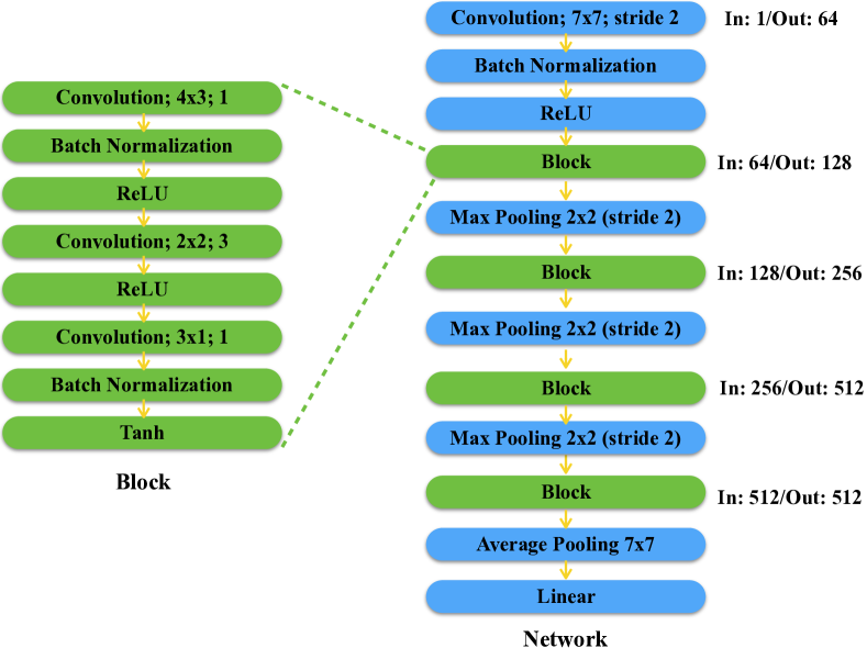
In Figure 1, we illustrate the selected block architecture based on Peephole-predicted accuracy. We also stack them in a similar manner to our scheme used in CIFAR-10. Note that this architecture is not generated by our algorithm but selected from randomly sampled validation architectures using Peephole.
| Conv | MP | AP | ReLU | Sigm | Tanh | |
|---|---|---|---|---|---|---|
| Conv | ||||||
| MP | ||||||
| AP | ||||||
| ReLU | ||||||
| Sigm | ||||||
| Tanh |
Details of Sampling Strategy.
Here we detail our configurations for Block-based Generation scheme. The whole process begins with a convolution layer whose kernel size is uniformly sampled from and the ratio of output/input channel number is uniformly sampled from . Then the construction will follow a Markov chain, i.e. we will choose the type of the next layer merely based on the current one. The transition matrix is shown in Table 1. Note that Batch Normalization is inserted right behind Convolution layers with the probability of . Thus it’s not shown in the table. Meanwhile, for computational consideration, we limit the depth of a block to less than layers and restrict the number of convolution layers within a block to less than .