Social Emotion Mining Techniques
for Facebook Posts Reaction Prediction

Abstract

As of February 2016 Facebook allows users to express their experienced emotions about a post by using five so-called ‘reactions’. This research paper proposes and evaluates alternative methods for predicting these reactions to user posts on public pages of firms/companies (like supermarket chains). For this purpose, we collected posts (and their reactions) from Facebook pages of large supermarket chains and constructed a dataset which is available for other researches. In order to predict the distribution of reactions of a new post, neural network architectures (convolutional and recurrent neural networks) were tested using pretrained word embeddings. Results of the neural networks were improved by introducing a bootstrapping approach for sentiment and emotion mining on the comments for each post. The final model (a combination of neural network and a baseline emotion miner) is able to predict the reaction distribution on Facebook posts with a mean squared error (or misclassification rate) of 0.135.

1 INTRODUCTION

The ability to accurately classify the sentiment of short sentences such as Facebook posts or tweets is essential to natural language understanding. In recent years, more and more users share information about their customer experience on social media pages related to (and managed by) the equivalent firms/companies. Generated data attracts a lot of research towards sentiment analysis with many applications in political science, social sciences, business, education, etc. [Ortigosa et al., 2014], [Feldman, 2013], [Troussas et al., 2013].

Customer experience (CX) represents a holistic perspective on customer encounters with a firm’s products or services. Thus, the more managers can understand about the experiences customers have with their product and service offerings, the more they can measure them again in the future to influence purchase decisions. The rise of social media analytics [Fan and Gordon, 2014] offers managers a tool to manage this process with customer opinion data being widely available on social media. Analysing Facebook posts can help firm managers to better manage posts by allowing customer care teams to reply faster to unsatisfied customers or maybe even delegate posts to employees based on their expertise. Also, it would be possible to estimate how the reply on a post affects the reaction from other customers. To our knowledge, no previous research work on predicting Facebook reaction posts exists.

The main goals and contributions of this paper are the following: (a) contribute a dataset which can be used for predicting reactions on Facebook posts, useful for both machine learners and marketing experts and (b) perform sentiment analysis and emotion mining to Facebook posts and comments of several supermarket chains by predicting the distribution of the user reactions. Firstly, sentiment analysis and emotion mining baseline techniques are utilized in order to analyse the sentiment/emotion of a post and its comments. Afterwards, neural networks with pretrained word embeddings are used in order to accurately predict the distribution of reactions to a post. Combination of the two approaches gives a working final ensemble which leaves promising directions for future research.

The remainder of the paper is organized as follows. Section 2 presents related work about sentiment and emotion analysis on short informal text like from Facebook and Twitter. The used dataset is described in Section 3, followed by the model (pipeline) description in Section 4. Section 5 presents the experimental results and finally, Section 6 concludes the paper and presents future research directions.

2 RELATED WORK

Deep learning based approaches have recently become more popular for sentiment classification since they automatically extract features based on word embeddings. Convolutional Neural Networks (CNN), originally proposed in [LeCun et al., 1998] for document recognition, have been extensively used for short sentence sentiment classification. [Kim, 2014] uses a CNN and achieves state-of-the art results in sentiment classification. They also highlight that one CNN layer in the model’s architecture is sufficient to perform well on sentiment classification tasks. Recurrent Neural Networks (RNN) and more specifically their variants Long Short Term Memory (LSTM) networks [Hochreiter and Schmidhuber, 1997] and Gated Recurrent Units (GRU) networks [Chung et al., 2014] have also been extensively used for sentiment classification since they are able to capture long term relationships between words in a sentence while avoiding vanishing and exploding gradient problems of normal recurrent network architectures [Hochreiter, 1998]. [Wang et al., 2014] proves that combining different architectures, such as CNN and GRU, in an ensemble learner improves the performance of individual base learners for sentiment classification, which makes it relevant for this research work as well.

Most of the work on short text sentiment classification concentrates around Twitter and different machine learning techniques [Wang et al., 2011], [Kouloumpis et al., 2011], [Saif et al., 2012], [Sarlan et al., 2014]. These are some examples of the extensive research already done on Twitter sentiment analysis. Not many approaches for Facebook posts exist, partly because it is difficult to get a labeled dataset for such a purpose.

Emotion lexicons like EmoLex [Mohammad and Turney, 2013] can be used in order to annotate a corpus, however, results are not satisfactory and this is the reason that bootstrapping techniques have been attempted in the past. For example, [Canales et al., 2016] propose such a technique which enhances EmoLex with synonyms and then combines word vectors [Mikolov et al., 2013] in order to annotate more examples based on sentence similarity measures.

Recently, [Tian et al., 2017] presented some first results which associate Facebook reactions with emojis but their analysis stopped there. [Pool and Nissim, 2016] utilized the actual reactions on posts in a distant supervised fashion to train a support vector machine classifier for emotion detection but they are not attempting at actually predicting the distribution of reactions.

Moreover, analysis of customer feedback is an area which gains interest for many companies over the years. Given the amount of text feedback available, there are many approaches around this topic, however none of them are handling the increasing amounts of information available through Facebook posts. For the sake of completeness, we highlight here some these approaches. Sentiment classification ([Pang et al., 2002], [Glorot et al., 2011b], [Socher et al., 2013]) deals only with the sentiment analysis (usually mapping sentiments to positive, negative and neutral (or other 5-scale classification) and similarly emotion classification ([Yang et al., 2007], [Wen and Wan, 2014] only considers emotions. Some work exists on Twitter data [Pak and Paroubek, 2010] but does not take into account the reactions of Facebook. Moreover, work has been conducted towards customer review analysis ([Yang and Fang, 2004], [Hu and Liu, 2004], [Cambria et al., 2013]) but none of them are dealing with the specific nature of Facebook (or social media in general).

In this work, we combine sentiment analysis and emotion mining techniques with neural network architectures in order to predict the distribution of reactions on Facebook posts and actually demonstrate that such an approach is feasible.

3 DATASET CONSTRUCTION

Our dataset consists out of Facebook posts on the customer service page of 12 US/UK big supermarket/retail chains, namely Tesco, Sainsbury, Walmart, AldiUK, The Home Depot, Target, Walgreens, Amazon, Best Buy, Safeway, Macys and publix. The vast majority of these posts are initiated by customers of these supermarkets. In addition to the written text of the posts, we also fetch the Facebook’s reaction matrix as well as the comments attached to this post made by other users. Such reactions only belong to the initial post, and not to replies to the post since the feature to post a reaction on a reply has only been introduced very recently (May 2017) and would result in either a very small dataset or an incomplete dataset. These reactions include like, love, wow, haha, sad, angry as shown in Figure 1. This form of communication was introduced by Facebook on February 24th, 2016 and allows users to express an ‘emotion’ towards the posted content.

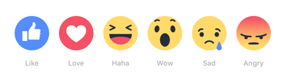
Figure 1: The Facebook reaction icons that users are able to select for an original post.

In total, there were more than 70,000 posts without any reaction, thus they were excluded from the dataset. Apart from this problem, people are using the ‘like’ reaction not only to show that they like what they see/read but also to simply tell others that they have seen this post or to show sympathy. This results in a way too often used ‘like’-reaction which is why likes could be ignored in the constructed dataset. So, instead of using all crawled data, the developed models will be trained on posts that have at least one other reaction than likes. After applying this threshold the size of the training set reduced from 70,649 to 25,969. The threshold of 1 is still not optimal since it leaves much space for noise in the data (e.g. miss-clicked reactions) but using a higher threshold will lead to extreme loss of data. Statistics on the dataset and on how many posts ‘survive’ by using different thresholds can be seen in Figure 2.

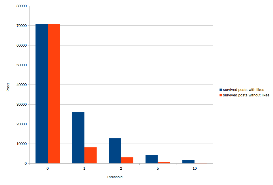
Figure 2: Amount of survived posts for different thresholds including/excluding likes

Exploratory analysis on the dataset shows that people tend to agree in the reactions they have to Facebook posts (which is consistent for building a prediction system), i.e. whenever there are more than one types of reactions they seem to be the same in a great degree (over 80 %) as can be seen in Figure 3. In addition, Figure 4 shows that even by excluding the like reaction, which seems to dominate all posts, the distribution of the reactions remains the same, even if the threshold of minimum reactions increases. Using all previous insights and the fact that there are 25,969 posts with at least one reaction and since the like reaction dominates the posts, we chose to include posts with at least one reaction which is not a like, leading to finally 8,103 posts. Full dataset is available and will be updated as it is curated and validated at the moment of the paper submission.

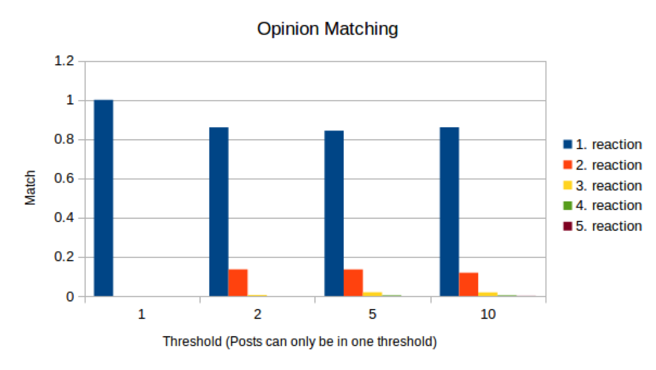
Figure 3: Reaction match when there is more than one type

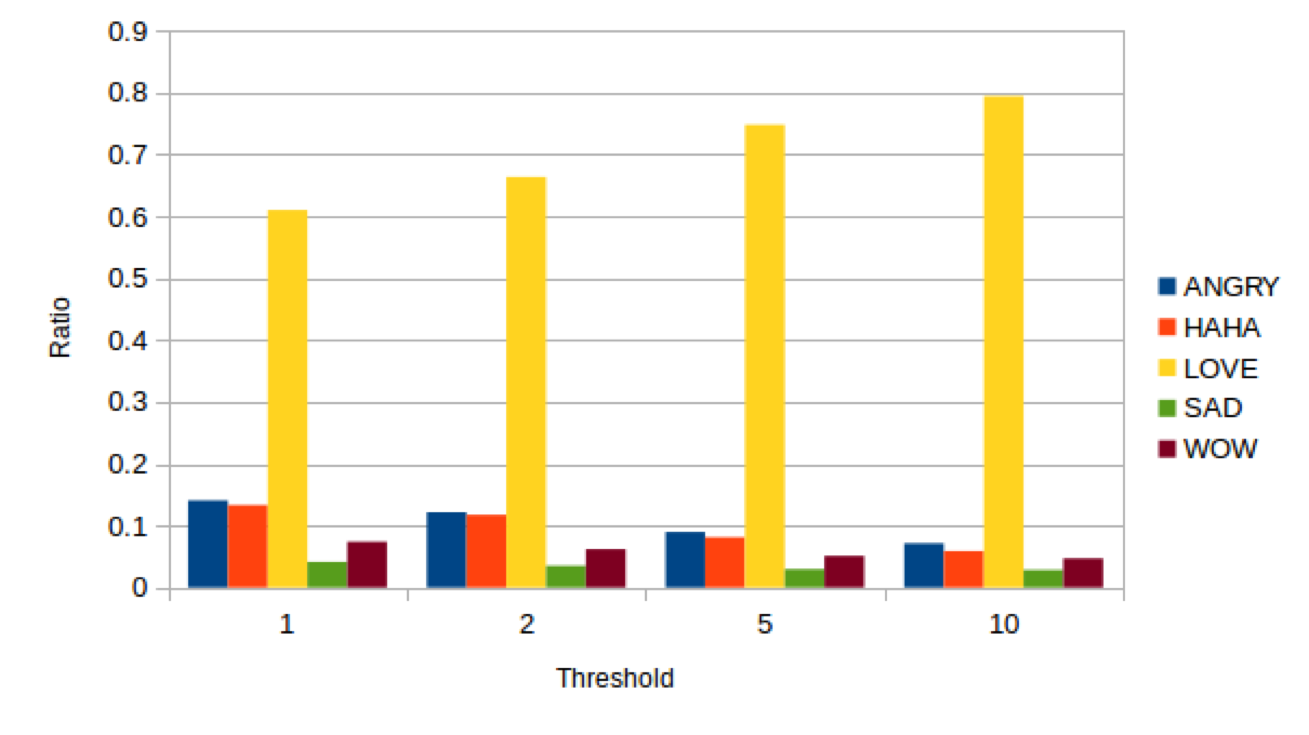
Figure 4: Distribution of reactions with different minimum thresholds

3.1 Pre-processing

Pre-processing on the dataset is carried out using the Stanford CoreNLP parser [Manning et al., 2014] and includes the following steps:

• Convert everything to lower case

• Replace URLs with “__URL__” as a generic token

• Replace user/profile links with “__AT_USER__” as a generic token

• Remove the hash from a hashtag reference (e.g. #hashtag becomes “hashtag”)

• Replace three or more occurrences of one character in a row with the character itself (e.g. “looooove” becomes ”love”)

• Remove sequences containing numbers (e.g. “gr34t”)

Afterwards, each post is split using a tokenizer based on spaces and after some stop-word filtering the final list of different tokens is derived. Since pre-processing on short text has attracted much attention recently [Singh and Kumari, 2016], we also demonstrate the effect of it on the developed models in the Experiments section.

4 REACTION DISTRIBUTION PREDICTION SYSTEM PIPELINE

In this Section, the complete prediction system is described. There are three core components: emotion mining applied to Facebook comments, artificial neural networks that predict the distribution of the reactions for a Facebook post and a combination of the two in the final prediction of the distribution of reactions.

4.1 Emotion mining

The overall pipeline of the emotion miner can be found in Figure 5.

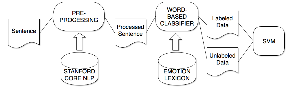
Figure 5: Emotion miner pipeline

The emotion lexicon that we utilize is created by [Mohammad and Turney, 2013] and is called NRC Emotion Lexicon (EmoLex). This lexicon consists of 14,181 words with eight basic emotions (anger, fear, anticipation, trust, surprise, sadness, joy, and disgust) associated with each word in the lexicon. It is possible that a single word is associated with more than one emotion. An example can be seen in Table 1. Annotations were manually performed by crowd-sourcing.

Table 1: Examples from EmoLex showing the emotion association to the words abuse and shopping.

	Anger	Anticipation	Disgust	Fear	Joy	Sadness	Surprise	Trust
abuse	1	0	1	1	0	1	0	0
shopping	0	1	0	0	1	0	1	1

Inspired by the approach of [Canales et al., 2016], EmoLex is extended by using WordNet [Fellbaum, 1998]: for every synonym found, new entries are introduced in EmoLex having the same emotion vector as the original words. By applying this technique the original database has increased in size from 14,181 to 31,485 words that are related to an emotion vector. The lexicon can then be used to determine the emotion of the comments to a Facebook post. For each sentence in a comment, the emotion is determined by looking up all words in the emotion database and the found emotion vectors are added to the sentence emotion vector. By merging and normalizing all emotion vectors, the final emotion distribution for a particular Facebook post, based on the equivalent comments, can be computed. However, this naive approach yielded poor results, thus several enhancements were considered, implemented and described in subsections 4.1.1-4.1.3.

4.1.1 Negation Handling

The first technique that was used to improve the quality of the mined emotions is negation handling. By detecting negations in a sentence, the ability to ‘turn’ this sentiment or emotion is provided. In this paper only basic negation handling is applied since the majority of the dataset contains only small sentences and this was proved to be sufficient for our goal. The following list of negations and pre- and suffixes are used for detection (based on work of [Farooq et al., 2016]):

Table 2: Negation patterns

Negations	no, not, rather, wont, never, none, nobody, nothing, neither, nor, nowhere, cannot, without, n’t
Prefixes	a, de, dis, il, im, in, ir, mis, non, un
Suffixes	less

The following two rules are applied:

1. The first rule is used when a negation word is instantly followed by an emotion-word (which is present in our emotion database).

2. The second rule tries to handle adverbs and past particle verbs (Part-of-Speech (POS) tags: RB, VBN). If a negation word is followed by one or more of these POS-tags and a following emotion-word, the emotion-word’s value will be negated. For example this rule would apply to ‘not very happy’.

There are two ways to obtain the emotions of a negated word:

1. Look up all combinations of negation pre- and suffixes together with the word in our emotion lexicon.

2. If there is no match in the lexicon a manually created mapping is used between the emotions and their negations. This mapping is shown in Table 3.

Table 3: Mapping between emotion and negated emotions.

	Anger	Anticipation	Disgust	Fear	Joy	Sadness	Surprise	Trust
Anger	0	0	0	0	1	0	0	0
Anticipation	0	0	0	0	1	0	1	0
Disgust	0	0	0	0	1	0	0	1
Fear	0	0	0	0	1	0	0	1
Joy	1	0	1	1	0	1	0	0
Sadness	0	0	0	1	0	0	0	0
Surprise	0	1	0	0	0	0	0	1
Trust	0	0	1	0	0	0	1	0

4.1.2 Sentence similarity measures

[Canales et al., 2016]’s approach is using word vectors [Mikolov et al., 2013] in order to calculate similarities between sentences and further annotate sentences. In the context of this paper, a more recent approach was attempted [Sanjeev Arora, 2017], together with an averaging word vector approach for comparison. [Sanjeev Arora, 2017] creates a representation for a whole sentence instead of only for one word as word2vec. The average word vector approach is summing up the word vector of each word and then taking the mean of this sum. To find a similarity between two sentences, one then uses the cosine similarity. Surprisingly, both approaches return comparable similarity scores. One main problem which occurred here is that two sentences with different emotions but with the same structure are measured as ‘similar’. This problem is exemplified with an example:

Sentence 1: "I really love your car."
Sentence 2: "I really hate your car."
Sentence2Vec similarity: 0.9278
Avg vector similarity: 0.9269

This high similarity is problematic since the emotions of the two sentences are completely different. Also, one can see that the two models output almost the same result and that there is no advantage by using the approach of [Sanjeev Arora, 2017] over the simple average word vector approach. Hence, the sentence similarity measure method to annotate more sentences is not suited for this emotion mining task because one would annotate positive emotions to a negative sentence and was not adapted for further use.

4.1.3 Classification of not annotated sentences

If after performing these enhancement steps there remain any non-emotion-annotated sentences, then a Support Vector Machine (SVM) is used to estimate the emotions of these sentences based on the existing annotations. The SVM is trained as a one-versus-all classifier with a linear kernel (8 models are trained, one for each emotion of EmoLex) and the TF-IDF model [Salton and Buckley, 1988] is used for providing the input features. Input consists of a single sentence as data (transformed using the TF-IDF model) and an array of 8 values representing the emotions as a label. With a training/test-split of 80%/20%, the average precision-recall is about 0.93. Full results of the SVM training can be seen in Figure 6 together with the precision-recall curve for all emotions. The result in this case was judged to be satisfactory in order to utilize it for the next step, which is the reaction prediction and is used as presented here.

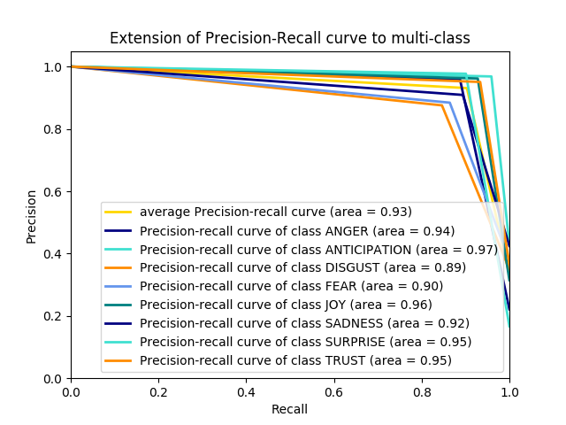
Figure 6: Precision-Recall (ROC) curve using a linear SVM in an one-versus-all classifier

4.2 Reaction distribution predictor

In order to predict the distribution of the post reactions, neural networks are built and trained using Tensorflow [Abadi et al., 2016]. Two networks were tested, based on literature research: a Convolutional Neural Network (CNN) and a Recurrent Neural Network (RNN) that uses LSTMs.

Both networks start with a word embedding layer. Since the analysed posts were written in English, the GloVe [Pennington et al., 2014] pretrained embeddings (with 50 as a vector dimension) were used. Moreover, posts are short texts and informal language is expected, thus we opted for using embeddings previously trained on Twitter data instead of the Wikipedia versions.

4.2.1 CNN

The CNN model is based on existing successful architectures (see [Kim, 2014]) but is adapted to give a distribution of reactions as an output. An overview of the used architecture is provided in Figure 7.

First issue to be handled with CNNs is that since they deal with variable length input sentences, padding is needed so as to ensure that all posts have the same length. In our case, we padded all posts to the maximum post length which also allows efficient batching of the data. In the example of Figure 7 the length of the sentence is 7 and each word $x_{i}$ is represented by the equivalent word vector (of dimension 50).

The convolutional layer is the core building block of a CNN. Common patterns in the training data are extracted by applying the convolution operation which in our case is limited into 1 dimension: we adjust the height of the filter, i.e. the number of adjacent rows (words) that are considered together (see also red arrows in Figure 7). These patterns are then fed to a pooling layer. The primary role of the pooling layer is to reduce the spatial dimensions of the learned representations (that’s why this layer is also known to perform downsampling). This is beneficial, since it controls for over-fitting but also allows for faster computations. Finally, the output of the pooling layer is fed to a fully-connected layer (with dropout) which has a softmax as output and each node corresponds to each predicted reaction (thus we have six nodes initially). However, due to discarding like reaction later on in the research stage, the effective number of output nodes was decreased to 5 (see Experiments). The softmax classifier computes a probability distribution over all possible reactions, thus provides a probabilistic and intuitive interpretation.

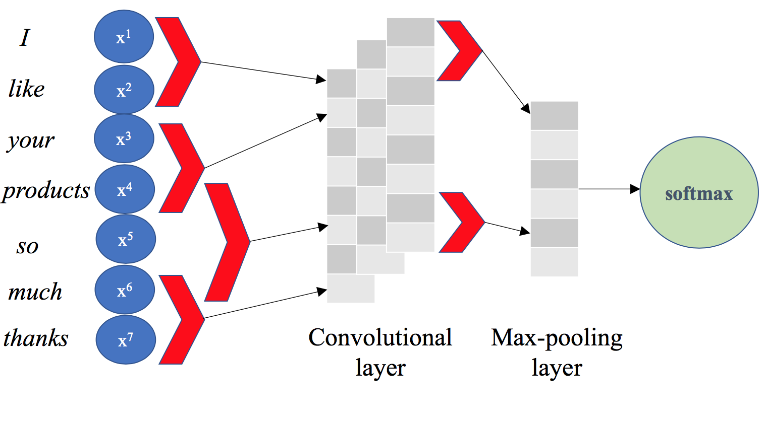
Figure 7: Convolutional network architecture example

4.2.2 RNN

Long short-term memory networks (LSTM) were proposed by [Hochreiter and Schmidhuber, 1997] in order to adress the issue of learning long-term dependencies. The LSTM maintains a separate memory cell inside it that updates and exposes its content only when deemed necessary, thus making it possible to capture content as needed. The implementation used here is inspired by [Graves, 2013] and an overivew is provided in Figure 8.

An LSTM unit (at each time step $t$) is defined as a collection of vectors: the input gate ($i_{t}$), the forget gate ($f_{t}$), the output gate ($o_{t}$), a memory cell ($c_{t}$) and a hidden state ($h_{t}$). Input is provided sequentially in terms of word vectors ($x_{t}$) and for each time step $t$ the previous time step information is used as input. Intuitively, the forget gate controls the amount of which each unit of the memory cell is replaced by new info, the input gate controls how much each unit is updated, and the output gate controls the exposure of the internal memory state.

In our case, the RNN model utilizes one recurrent layer (which has 50 LSTM cells) and the rest of the parameters are chosen based on current default working architectures. The output then comes from a weighted fully connected 6-(or 5, depending on the number of reactions)-class softmax layer. Figure 8 explains the idea of recurrent architecture based on an input sequence of words.

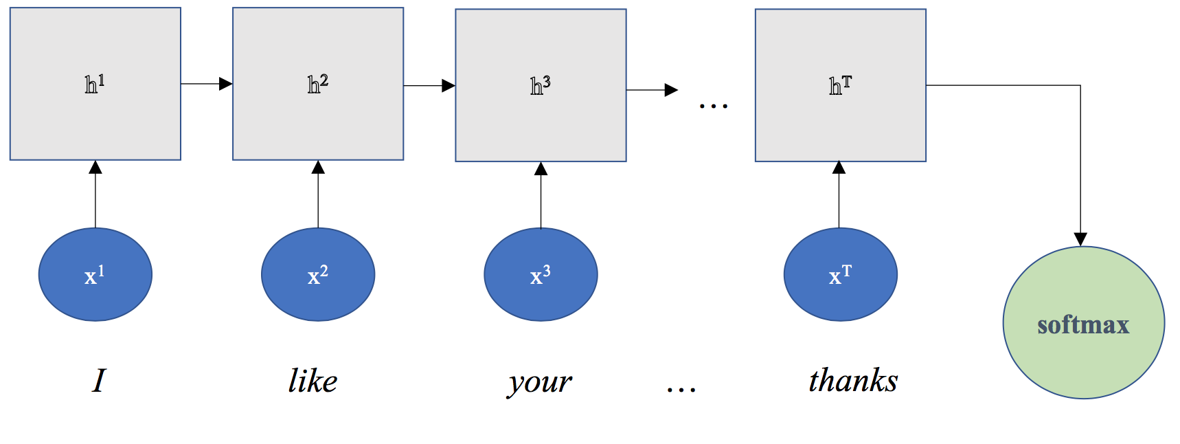
Figure 8: Recurrent network architecture example

4.3 Prediction ensemble

The final reaction ratio prediction is carried out by a combination of the neural networks and the mined emotions on the post/comments. For a given post, both networks provide an estimation of the distributions, which are then averaged and normalised. Next, emotions from the post and the comments are extracted following the process described in Section 4.1. The ratio of estimations and emotions are combined into a single vector which is then computed through a simple linear regression model, which re-estimates the predicted reaction ratios. The whole pipeline combining the emotion miner and the neural networks can be seen in Figure 9 and experimental results are presented in the next Section.

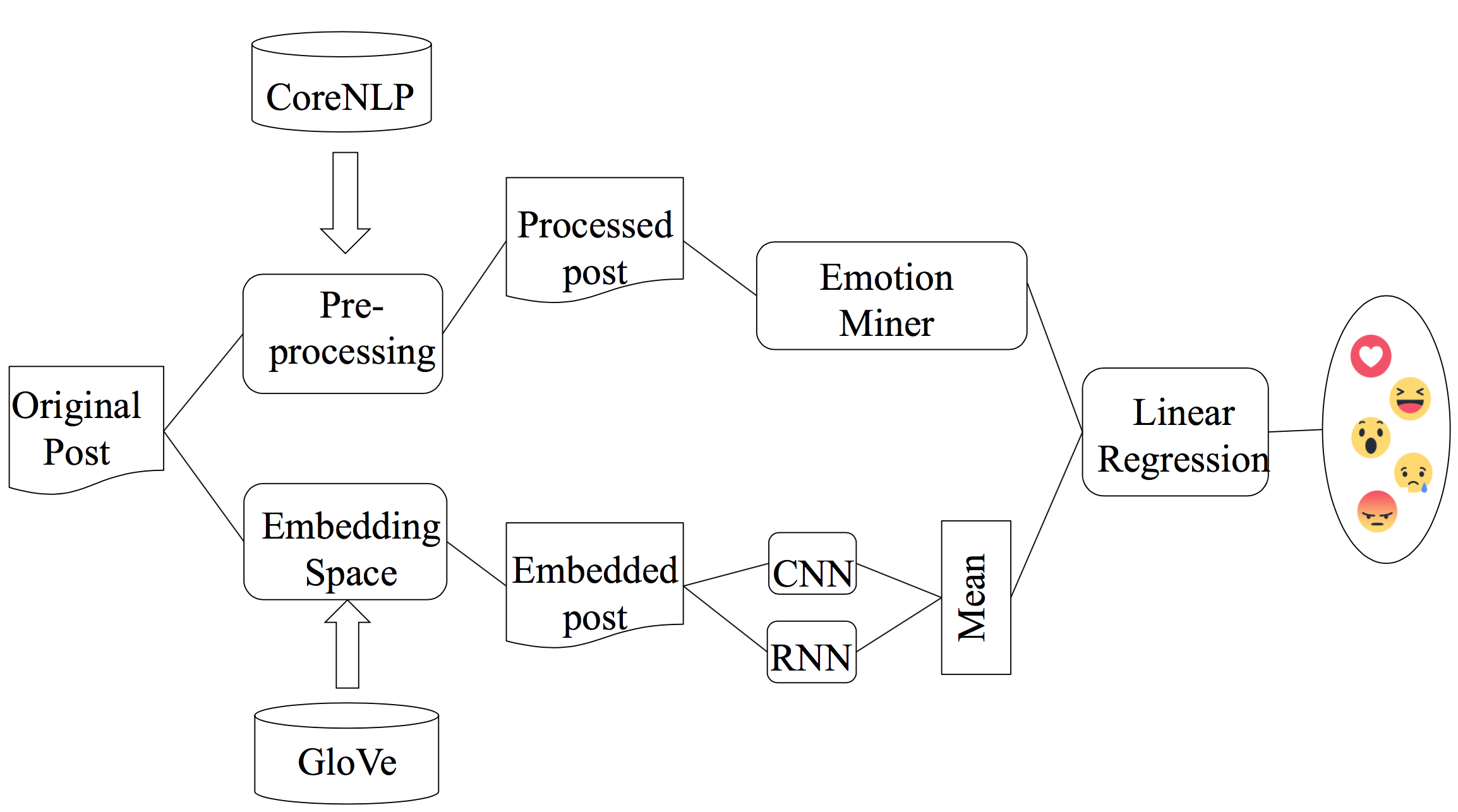
Figure 9: Pipeline for final prediction of reaction distributions

5 EXPERIMENTS

Several experiments were conducted in order to assess different effects on the reaction distribution prediction. Firstly, the effect of pre-processing on posts is examined in subsection 5.1. Since Facebook reactions were not introduced too long ago, a lot of posts in the dataset still contain primarily like reactions. This might lead to uninteresting results as described in the Dataset Section and in Subsection 5.2. Finally, Subsection 5.3 discusses the training with respect to the mean squared error (MSE) for CNN and RNN models, as well as the effect of the ensembled approach.

As mentioned before, both networks utilized the GloVe pre-trained embeddings (with size 50). Batch size was set to 16 for the CNN and 100 for the RNN/LSTM.

CNN used 40 filters for the convolution (with varying height sizes from 3 to 5), stride was set to 1 and padding to the maximum post length was used. Rectified Linear Unit (ReLU) [Glorot et al., 2011a] activation function was used.

Learning rate was set to 0.001 and dropout was applied to both networks and performance was measured by the cross entropy loss with scores and labels with L2-regularization [Masnadi-Shirazi and Vasconcelos, 2009]. Mean Squared Error (MSE) is used in order to assess successful classifications (which effectively means that every squared error will be a 1) and in the end MSE is just the misclassification rate of predictions.

5.1 Raw vs Pre-processed Input

In order to assess the effect of pre-processing on the quality of the trained models, two versions for each neural network were trained. One instance was trained without pre-processing the dataset and the other instance was trained with the pre-processed dataset. Results are cross-validated and here the average values are reported. Figure 10 indicates that overall the error was decreasing or being close to equal (which is applicable for both CNN and RNN). The x-axis represents the minimum number of ‘non-like’ reactions in order to be included in the dataset. It should be noted that these models were trained on the basis of having 6 outputs (one for each reaction), thus the result might be affected by the skewed distribution over many ‘like’ reactions. This is the reason that the pre-processed version of CNN performs very well for posts with 5 minimum reactions and very bad for posts with 10 minimum reactions In addition, the variance for the different cross-validation results was high. In the next subsection we explore what happens after the removal of ‘like’ reactions.

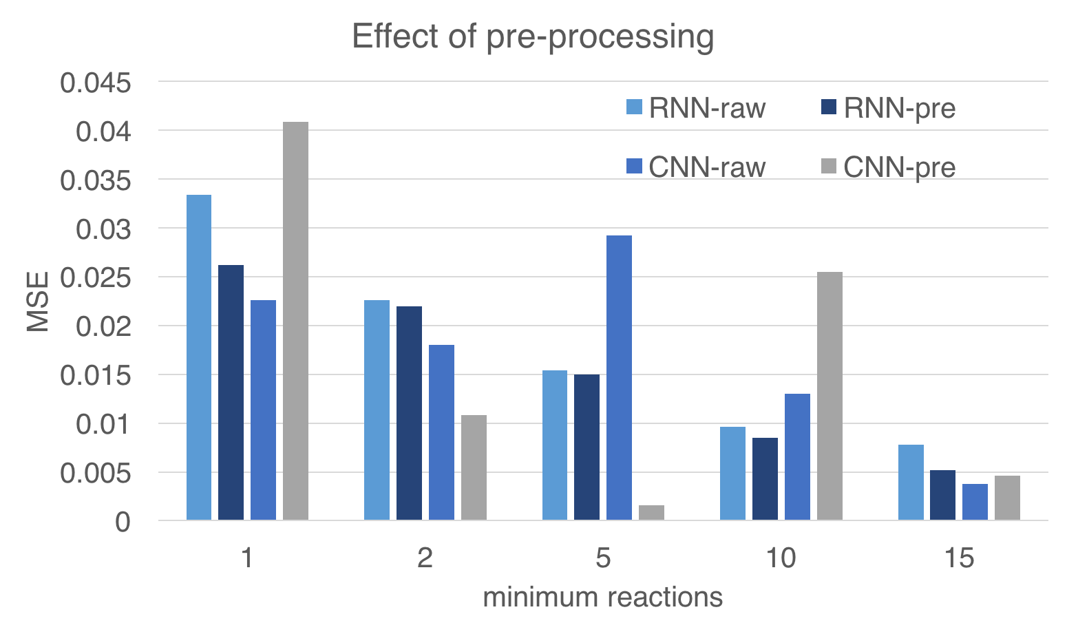
Figure 10: Effect of pre-processing on different models

5.2 Exclusion of like reactions

Early results showed that including the original like reaction in the models would lead to meaningless results. The huge imbalanced dataset led to predicting a 100% ratio for the like reaction. In order to tackle this issue, the like reactions are not fed into the models during the training phase (moreover the love reaction can be used for equivalent purposes, since they express similar emotions). Figure 11 shows an increase of the error when the likes are ignored. The explanation for this increase is related to heavily unbalanced distribution of like reactions: Although there is an increase in the error, predictions now are more meaningful than always predicting a like ratio close to 100%. After all, it is the relative reaction distribution that we are interested in predicting.

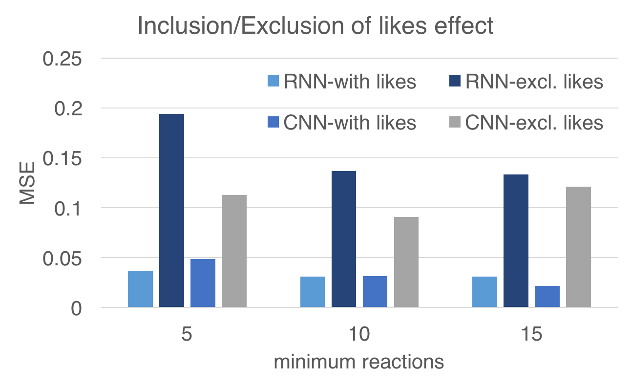
Figure 11: Effect of inclusion/exclusion of likes on different models

5.3 Ensemble performance

Table 4 summarizes the testing error for the CNN and RNN with respect to the same split dataset and by also taking the validation error into account. One can see that RNN performs better than CNN, although it requires additional training time. Results are cross-validated on 10 different runs and variances are presented in the Table as well.

Table 4: RNN and CNN comparison after cross-validation

	MSE	# Epochs
CNN	0.186 ($\pm 0.023$)	81
RNN	0.159 ($\pm 0.017$)	111

Combined results for either of the networks and the emotion miner can be seen in Figure 12. The networks themselves have the worst results but an average combination of both is able to achieve a better result. Optimal result is achieved by the emotions + cnn combination, although this difference is not significant than other combinations. These results can be boosted by optimizing the hyperparameters of the networks and also by varying different amount of posts. As a conclusion one can say that using emotions to combine them with neural network output improves the results of prediction.

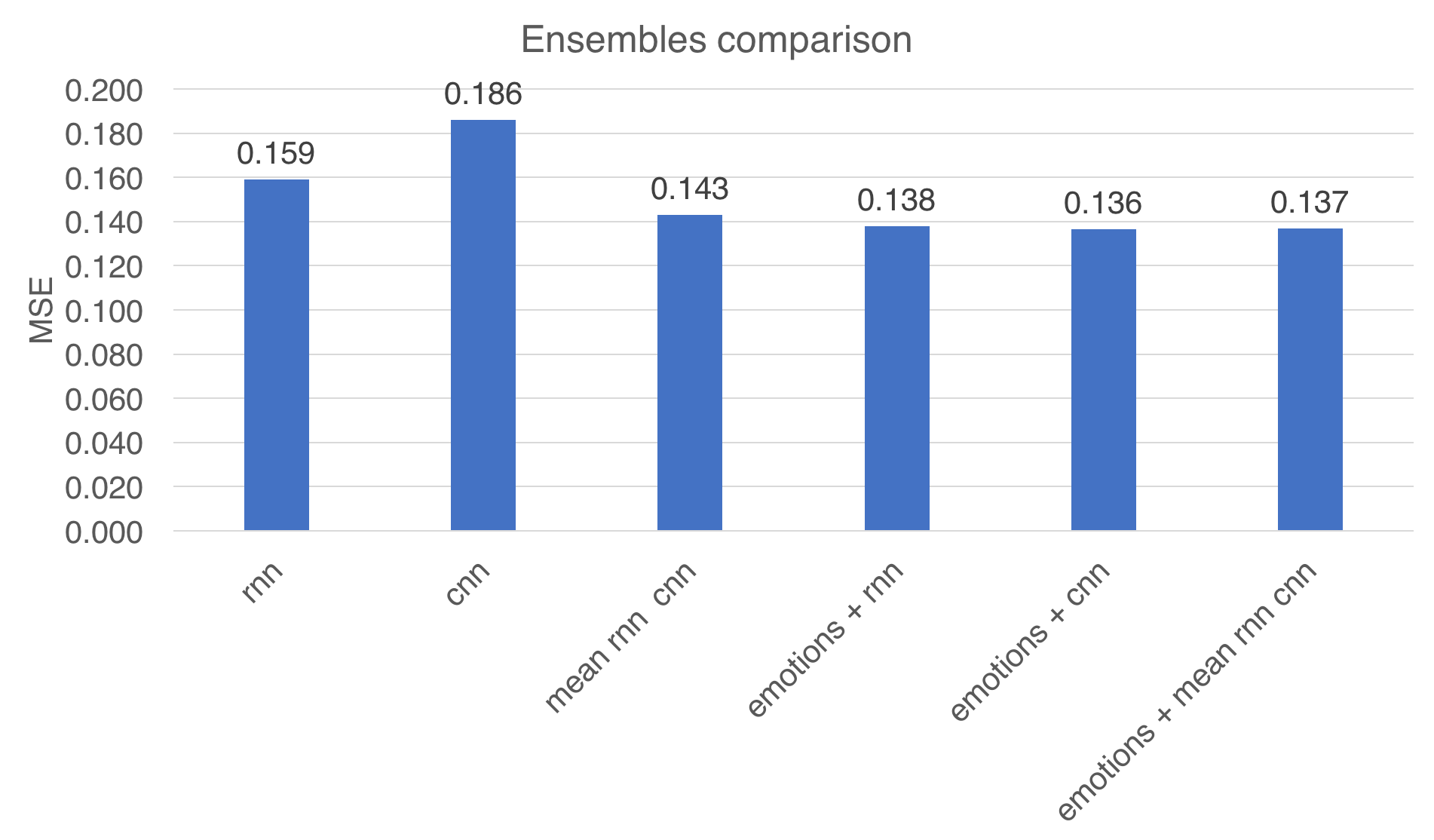
Figure 12: Performance results for different combinations of the neural networks and emotions.

Finally, we present a simple, yet effective visualization environment which highlights the results of the current paper, that can be found in Figure 13. In this figure, one can see at the input field of the Facebook post on the top and then four different result panels: the first one shows the reaction distribution, the second panel shows the proportions of the eight emotions, the third panel highlights the emotions (and by hovering one can see the total shows the overall distribution (vector of eight) and the fourth panel shows the highlighting of the sentiments.

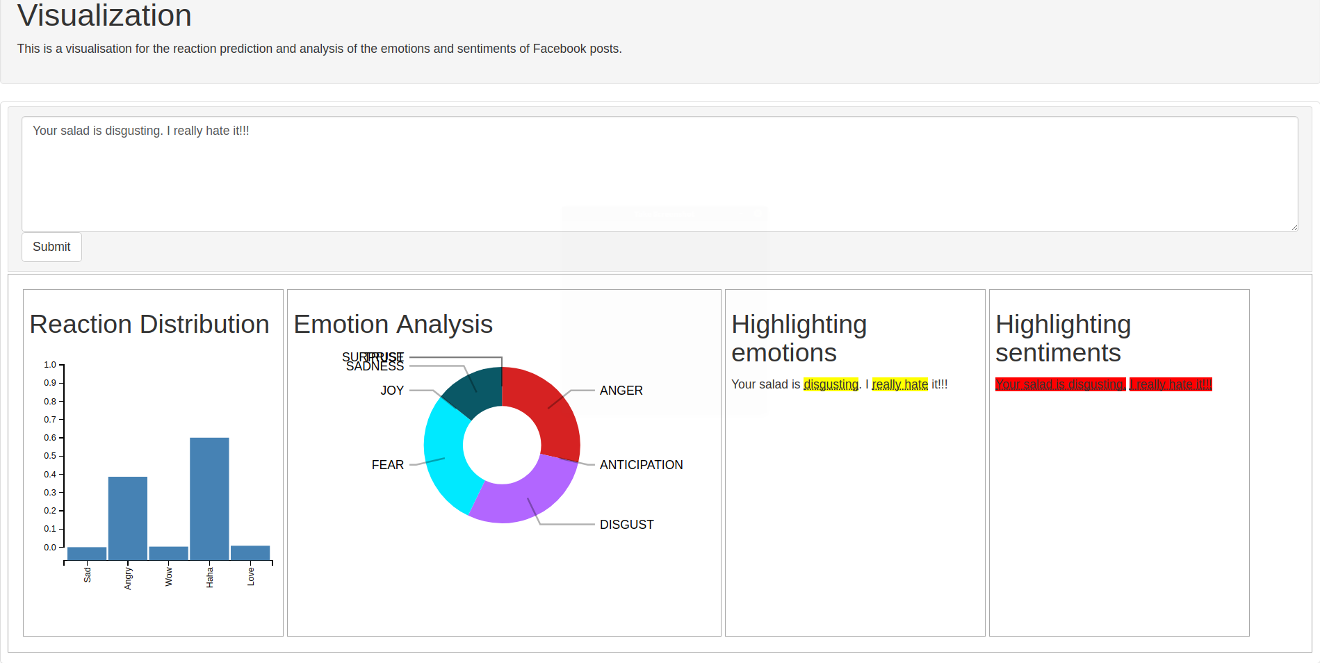
Figure 13: Example visualisation

6 Conclusion

In this paper, a framework for predicting the Facebook post reaction distribution was presented, trained on a customer service dataset from several supermarket Facebook posts. This study revealed that a baseline sentiment miner can be used in order to detect a post sentiment/emotion. Afterwards, these results can be combined with the output of neural network models to predict the Facebook reactions. While there has been a lot of research around sentiment analysis, emotion mining is still mostly uncharted territory and this work also contributes to this direction. The used dataset is available for other researchers and can be also used as a baseline for performing further experiments. In addition, a more accurate evaluation of the emotion miner can be conducted by using the MPQA corpus [Deng and Wiebe, 2015].

Facebook reaction predictions can clearly enhance customer experience analytics. Most companies are drowned in social media posts, thus a system that identifies the emotion/reaction prediction of a post in almost real-time can be used to provide effective and useful feedback to customers and improve their experience. So far in the dataset, the reaction of the page owner has not been included but this could be useful information on how the post was addressed (or could be addressed).

Future work includes working towards refining the architectures of the neural networks used. Moreover, one of the next steps is to implement a network that predicts the (absolute) amount of reactions (and not just the ratio). This number is of course susceptible to external parameters (e.g. popularity of the post/poster, inclusion of other media like images or external links, etc.), so another direction would be to include this information as well. More specifically, the combination of images and text can reveal possible synergies in the vision and language domains for sentiment/emotion related tasks.

REFERENCES

- Abadi et al., 2016 Abadi, M., Agarwal, A., Barham, P., Brevdo, E., Chen, Z., Citro, C., Corrado, G. S., Davis, A., Dean, J., Devin, M., et al. (2016). Tensorflow: Large-scale machine learning on heterogeneous distributed systems. arXiv preprint arXiv:1603.04467.
- Cambria et al., 2013 Cambria, E., Schuller, B., Xia, Y., and Havasi, C. (2013). New avenues in opinion mining and sentiment analysis. IEEE Intelligent Systems, 28(2):15–21.
- Canales et al., 2016 Canales, L., Strapparava, C., Boldrini, E., and Martínez-Barco, P. (2016). Exploiting a bootstrapping approach for automatic annotation of emotions in texts. 2016 IEEE International Conference on Data Science and Advanced Analytics (DSAA), pages 726–734.
- Chung et al., 2014 Chung, J., Gulcehre, C., Cho, K., and Bengio, Y. (2014). Empirical evaluation of gated recurrent neural networks on sequence modeling. arXiv preprint arXiv:1412.3555.
- Deng and Wiebe, 2015 Deng, L. and Wiebe, J. (2015). Mpqa 3.0: An entity/event-level sentiment corpus. In Mihalcea, R., Chai, J. Y., and Sarkar, A., editors, HLT-NAACL, pages 1323–1328. The Association for Computational Linguistics.
- Fan and Gordon, 2014 Fan, W. and Gordon, M. D. (2014). The power of social media analytics. Communications of the ACM, 57(6):74–81.
- Farooq et al., 2016 Farooq, U., Nongaillard, A., Ouzrout, Y., and Qadir, M. A. (2016). Negation Handling in Sentiment Analysis at Sentence Level. In Internation Conference on Information Management, Londres, United Kingdom.
- Feldman, 2013 Feldman, R. (2013). Techniques and applications for sentiment analysis. Communications of the ACM, 56(4):82–89.
- Fellbaum, 1998 Fellbaum, C. (1998). WordNet: An Electronic Lexical Database. Bradford Books.
- Glorot et al., 2011a Glorot, X., Bordes, A., and Bengio, Y. (2011a). Deep sparse rectifier neural networks. In Proceedings of the Fourteenth International Conference on Artificial Intelligence and Statistics, pages 315–323.
- Glorot et al., 2011b Glorot, X., Bordes, A., and Bengio, Y. (2011b). Domain adaptation for large-scale sentiment classification: A deep learning approach. In Proceedings of the 28th international conference on machine learning (ICML-11), pages 513–520.
- Graves, 2013 Graves, A. (2013). Generating sequences with recurrent neural networks. arXiv preprint arXiv:1308.0850.
- Hochreiter, 1998 Hochreiter, S. (1998). The vanishing gradient problem during learning recurrent neural nets and problem solutions. International Journal of Uncertainty, Fuzziness and Knowledge-Based Systems, 6(02):107–116.
- Hochreiter and Schmidhuber, 1997 Hochreiter, S. and Schmidhuber, J. (1997). Long short-term memory. Neural computation, 9(8):1735–1780.
- Hu and Liu, 2004 Hu, M. and Liu, B. (2004). Mining and summarizing customer reviews. In Proceedings of the tenth ACM SIGKDD international conference on Knowledge discovery and data mining, pages 168–177. ACM.
- Kim, 2014 Kim, Y. (2014). Convolutional neural networks for sentence classification. CoRR, abs/1408.5882.
- Kouloumpis et al., 2011 Kouloumpis, E., Wilson, T., and Moore, J. D. (2011). Twitter sentiment analysis: The good the bad and the omg! Icwsm, 11(538-541):164.
- LeCun et al., 1998 LeCun, Y., Bottou, L., Bengio, Y., and Haffner, P. (1998). Gradient-based learning applied to document recognition. Proceedings of the IEEE, 86(11):2278–2324.
- Manning et al., 2014 Manning, C. D., Surdeanu, M., Bauer, J., Finkel, J., Bethard, S. J., and McClosky, D. (2014). The Stanford CoreNLP natural language processing toolkit. In Association for Computational Linguistics (ACL) System Demonstrations, pages 55–60.
- Masnadi-Shirazi and Vasconcelos, 2009 Masnadi-Shirazi, H. and Vasconcelos, N. (2009). On the design of loss functions for classification: theory, robustness to outliers, and savageboost. In Advances in neural information processing systems, pages 1049–1056.
- Mikolov et al., 2013 Mikolov, T., Chen, K., Corrado, G., and Dean, J. (2013). Efficient estimation of word representations in vector space. arXiv preprint arXiv:1301.3781.
- Mohammad and Turney, 2013 Mohammad, S. M. and Turney, P. D. (2013). Crowdsourcing a word-emotion association lexicon. 29(3):436–465.
- Ortigosa et al., 2014 Ortigosa, A., Martín, J. M., and Carro, R. M. (2014). Sentiment analysis in facebook and its application to e-learning. Computers in Human Behavior, 31:527–541.
- Pak and Paroubek, 2010 Pak, A. and Paroubek, P. (2010). Twitter as a corpus for sentiment analysis and opinion mining. In LREc, volume 10.
- Pang et al., 2002 Pang, B., Lee, L., and Vaithyanathan, S. (2002). Thumbs up?: sentiment classification using machine learning techniques. In Proceedings of the ACL-02 conference on Empirical methods in natural language processing-Volume 10, pages 79–86. Association for Computational Linguistics.
- Pennington et al., 2014 Pennington, J., Socher, R., and Manning, C. D. (2014). Glove: Global vectors for word representation. In Empirical Methods in Natural Language Processing (EMNLP), pages 1532–1543.
- Pool and Nissim, 2016 Pool, C. and Nissim, M. (2016). Distant supervision for emotion detection using facebook reactions. arXiv preprint arXiv:1611.02988.
- Saif et al., 2012 Saif, H., He, Y., and Alani, H. (2012). Semantic sentiment analysis of twitter. The Semantic Web–ISWC 2012, pages 508–524.
- Salton and Buckley, 1988 Salton, G. and Buckley, C. (1988). Term-weighting approaches in automatic text retrieval. Information processing & management, 24(5):513–523.
- Sanjeev Arora, 2017 Sanjeev Arora, Yingyu Liang, T. M. (2017). A simple but tough-to-beat baseline for sentence embeddings.
- Sarlan et al., 2014 Sarlan, A., Nadam, C., and Basri, S. (2014). Twitter sentiment analysis. In Information Technology and Multimedia (ICIMU), 2014 International Conference on, pages 212–216. IEEE.
- Singh and Kumari, 2016 Singh, T. and Kumari, M. (2016). Role of text pre-processing in twitter sentiment analysis. Procedia Computer Science, 89:549–554.
- Socher et al., 2013 Socher, R., Perelygin, A., Wu, J., Chuang, J., Manning, C. D., Ng, A., and Potts, C. (2013). Recursive deep models for semantic compositionality over a sentiment treebank. In Proceedings of the 2013 conference on empirical methods in natural language processing, pages 1631–1642.
- Tian et al., 2017 Tian, Y., Galery, T., Dulcinati, G., Molimpakis, E., and Sun, C. (2017). Facebook sentiment: Reactions and emojis. SocialNLP 2017, page 11.
- Troussas et al., 2013 Troussas, C., Virvou, M., Espinosa, K. J., Llaguno, K., and Caro, J. (2013). Sentiment analysis of facebook statuses using naive bayes classifier for language learning. In Information, Intelligence, Systems and Applications (IISA), 2013 Fourth International Conference on, pages 1–6. IEEE.
- Wang et al., 2014 Wang, G., Sun, J., Ma, J., Xu, K., and Gu, J. (2014). Sentiment classification: The contribution of ensemble learning. Decision support systems, 57:77–93.
- Wang et al., 2011 Wang, X., Wei, F., Liu, X., Zhou, M., and Zhang, M. (2011). Topic sentiment analysis in twitter: a graph-based hashtag sentiment classification approach. In Proceedings of the 20th ACM international conference on Information and knowledge management, pages 1031–1040. ACM.
- Wen and Wan, 2014 Wen, S. and Wan, X. (2014). Emotion classification in microblog texts using class sequential rules. In AAAI, pages 187–193.
- Yang et al., 2007 Yang, C., Lin, K. H.-Y., and Chen, H.-H. (2007). Emotion classification using web blog corpora. In Web Intelligence, IEEE/WIC/ACM International Conference on, pages 275–278. IEEE.
- Yang and Fang, 2004 Yang, Z. and Fang, X. (2004). Online service quality dimensions and their relationships with satisfaction: A content analysis of customer reviews of securities brokerage services. International Journal of Service Industry Management, 15(3):302–326.