Anomalous dynamics triggered by a non-convex equation of state in relativistic flows

Abstract

The non-monotonicity of the local speed of sound in dense matter at baryon number densities much higher than the nuclear saturation density ($n_{0}\approx 0.16\,$fm^-3) suggests the possible existence of a non-convex thermodynamics which will lead to a non-convex dynamics. Here, we explore the rich and complex dynamics that an equation of state (EoS) with non-convex regions in the pressure-density plane may develop as a result of genuinely relativistic effects, without a classical counterpart. To this end, we have introduced a phenomenological EoS, whose parameters can be restricted heeding to causality and thermodynamic stability constraints. This EoS shall be regarded as a toy-model with which we may mimic realistic (and far more complex) EoS of practical use in the realm of Relativistic Hydrodynamics.

1 Introduction

The complexity of the numerical models based upon a fluid description of the physical constituents (i.e., based upon a hydrodynamic or magnetohydrodynamic modeling) has grown pace to pace with the sustained increase of computational power available to the scientific and engineering community. Among other factors, the equation of state (EoS) employed sets the degree of realism with which physical systems are modeled. The EoS is a constitutive relation, which provides the closure to the sets of balance laws that account for the conservation of various basic quantities of the system (e.g., mass, momentum, energy, magnetic flux, etc.). There has been a progressive shift from assuming that the underlying fluid was governed by a simple EoS with, e.g., a constant adiabatic index, $\gamma$, to a more realistic microphysical description, where a general EoS, allowing for thermal and/or chemical processes, is decisive to shape both the thermodynamics and the dynamics of the flows. Numerous are the fields in which a complex EoS is needed. For instance, in Astrophysics, the treatment of the interstellar medium in the process of fragmentation of self-gravitating molecular clouds (e.g., Spaans & Silk, 2000; Li et al., 2003; Jappsen et al., 2005); the thermo-chemical evolution of the primordial stars (e.g., Yoshida et al., 2006; Glover & Abel, 2008; Clark et al., 2011; Greif et al., 2011); the envelopes of young planets embedded in protoplanetary disks (D’Angelo & Bodenheimer, 2013; Roth & Kasen, 2015); the spectral modeling of stellar atmospheres (e.g., Asplund et al., 1999; Collet et al., 2007); the stellar evolution (e.g., Kippenhahn & Weigert, 1990; Rauscher et al., 2002); the ionization of cold interstellar neutral gas as shock waves heat it (e.g., Flower et al., 2003; Vaidya et al., 2015), etc. However, complex EoSs are not restricted to astrophysics or plasma physics. They are also common in material processing, industrial frameworks and in the study of dense gas near the liquid-vapor saturation curve (Menikoff, 2007; Thompson & Lambrakis, 1973).

The convexity of any EoS is mathematically defined in terms of the value of the fundamental derivative, $\mathcal{G}$ (see Sect. 3). The fundamental derivative measures the convexity of the isentropes in the $p-\rho$ plane (where $p$ is the pressure and $\rho$ the rest-mass density). If ${\cal G}>0$, isentropes in the $p-\rho$ plane are convex, leading to expansive rarefaction waves and compressive shocks (Thompson, 1971; Rezzolla & Zanotti, 2013). This is the usual regime in which many astrophysical scenarios develop. However, some EoSs may display regimes in which ${\cal G}<0$, i.e., the EoS is non-convex. The non-convexity of isentropes in the$p-\rho$ plane yield, e.g., compressive rarefaction waves and expansive shocks. These non-classical or exotic phenomena have been observed experimentally (Cinnella & Congedo, 2007; Cinnella et al., 2011).

Prototype cases described by an extremely complex EoS involve systems where matter is so compact that its density is close to the nuclear saturation density ($n_{0}\approx 0.15-0.16$ fm^-3). The properties of the EoS for dense matter have a crucial influence in many different problems in Astrophysics and Nuclear Physics, some of which are: (1) the equilibrium and dynamics of compact stars (e.g., Baumgarte et al., 2000; Hempel et al., 2012; Banik et al., 2014), (2) the merger of compact objects (e.g., Kiuchi et al., 2009; Hotokezaka et al., 2011; Bauswein et al., 2014; Takami et al., 2014), (3) the evolution of the early Universe (e.g., Muñoz & Kamionkowski, 2015; Borsanyi et al., 2016), (4) the collision of heavy ions (e.g., Laine & Schröder, 2006; Nonaka & Bass, 2007; Luzum & Romatschke, 2008), etc. In spite of the important efforts (theoretical and experimental) the nuclear physicists and astrophysicists communities are still far from having an accurate knowledge of the properties of the EoS for dense matter (i.e., a fundamental physical issue).

At densities much higher than $n_{0}$ nuclear/hadronic matter undergoes a transition into a quark-gluon plasma (QGP). The nature of the finite-temperature QCD transition (first-order, second-order or analytic crossover) remains ambiguous (Aoki et al., 2006). Two groups, the HotQCD Collaboration (Bazavov et al., 2014) and the Wuppertal-Budapest Collaboration (Borsányi et al., 2014), have reported results - using QCD lattice techniques - about the EoS of the QGP that characterizes the transition from the hadronic phase into the QGP phase. Their findings in the continuum extrapolated EoS favor the crossover nature of the transition. In the phenomenologically relevant range of temperature, $130-400\,$MeV, the results from both groups show similarities with regard to the trace anomaly, pressure, energy density and entropy density. The energy density in the crossover region, $145\leq T\text{(MeV)}\leq 163$, is a factor of about $(1.2-3.1)$ times the nuclear saturation density. Remarkably, within the former temperature range the square of the sound speed, $c_{\rm s}^{2}$, is non-monotonic, displaying a minimum at $T_{c^{2}_{\rm s,min}}\approx 145-150\,$MeV. From that minimum and up to $T\simeq 200$ MeV, $c_{\rm s}^{2}<c^{2}/3$, where $c$ is the speed of light in vacuum. Following a different strategy, which combines the knowledge of the EoS of hadronic matter at low densities with the observational constraints on the masses of neutron stars, Bedaque & Steiner (2015) have concluded that the sound speed of dense matter is a non-monotonic function of density. In dense matter, the non-monotonicity of the speed of sound can also result from the behaviour of the adiabatic index (see definition below) in, e.g., the Skyrme Lyon (SLy; Chabanat et al. 1997, 1998) and in the Friedman Pandharipande Skyrme (FPS; Pandharipande & Ravenhall 1989) EoSs (see Fig. 5 in  Haensel & Potekhin 2004 and Fig. 1 below). More recently, Shen et al. (2011) have shown the non-monotonic behaviour of the adiabatic index for various EoSs broadly used in numerical simulations of core collapse, supernovae and compact object mergers (see their Fig. 9). Again, we remark that, beyond the disputable dip in the adiabatic index below $n_{0}$, which is typically attributed to the phase transition from non-uniform to uniform matter, all the equations of state compared in Shen et al. (2011) show that there is a range of densities above $n_{0}$ such that the adiabatic index decreases with density. Thus, the non-monotonicity of the adiabatic index (likewise, of the sound speed) should be considered as a genuine feature of matter at a few times the nuclear saturation density. Under such conditions, and particularly if there are phase transitions to exotic components, we advance that the fundamental derivative (see Sect. 3) could be negative, implying that the EoS be non-convex in that regime.

In Sec. 2 we show the equations of special relativistic hydrodynamics (SRHD) and recap their spectral properties for the readers benefit. Though these concepts are not new, they serve for the purpose of linking the convexity properties of the system of SRHD equations to its characteristic structure and to the convexity of the EoS. Studying the dynamics and thermodynamics of a realistic, state-of-the-art, non-convex EoS in a transrelativistic regime is a difficult task, in which obtaining any analytic insight is doubtful. Thus, we propose to illustrate the potential effects that a non-convex EoS may produce on both the thermodynamics and the dynamics of relativistic models with a phenomenological (analytic and very simple) EoS. This EoS has the virtue of mimicking the loss of convexity resulting from a non-monotonic behaviour of the adiabatic index with density, while at the same time be simple enough to gain a deeper physical insight in a number of phenomena of interest (Sect. 3). As we shall see, it is possible to tune the parameters of this phenomenological EoS to emulate the behaviour of the sound speed in very dense plasma (above nuclear matter density). The main focus of this work will be to carefully examine the regime in which purely relativistic effects determine the non-convex evolution of prototype relativistic Riemann problems of flows obeying our phenomenological EoS (Sect. 4). Since the relativistic effects we discuss here are independent of the numerical methods employed to solve the equations of SRHD, we defer for a follow up paper the comprehensive study of the numerical approximation of the non-convex special relativistic flows, governed by the current EoS, through the design of novel shock capturing schemes and a set of numerical experiments (Marquina et al., 2017). Our main conclusions will be summarized in Sect. 5.

2 The equations of SRHD

The equations of SRHD correspond to the conservation of rest-mass and energy-momentum of a fluid. In a flat space-time and Cartesian coordinates, these equations read (e.g., Font et al., 1994; Aloy et al., 1999):

$$J^{\mu}_{\,\,\,\,,\mu}=0,$$ (1)

$$T^{\mu\nu}_{\,\,\,\,\,\,,\mu}=0,$$ (2)

where subscripts $(\,_{,\mu}\,)$ denote the partial derivative with respect to the corresponding coordinate, $(t,x,y,z)$, and the standard Einstein sum convention is assumed. $J^{\mu}$ and $T^{\mu\nu}$ are the four-current density of rest mass and the energy-momentum tensor, respectively,

$$J^{\mu} =\rho u^{\mu},$$ (3)

$$T^{\mu\nu} =\rho hu^{\mu}u^{\nu}+\eta^{\mu\nu}p.$$ (4)

$\rho$ is the proper rest-mass density, $h=1+\varepsilon+p/\rho$ is the specific enthalpy, $\varepsilon$ is the specific internal energy, $p$ is the thermal pressure, and $\eta^{\mu\nu}$ is the Minkowski metric of the space-time where the fluid evolves. Throughout the paper we use units in which the speed of light is $c=1$. The four-vector representing the fluid velocity, $u^{\mu}$, satisfies the condition $u^{\mu}u_{\mu}=-1$.

The system formed by Eqs. (1) and (2) can be written in explicit conservation form as follows

$$\frac{\partial{\bf U}}{\partial t}+\frac{\partial{\bf F}^{i}}{\partial x^{i}}=0$$ (5)

where ${\bf V}=(\rho,v^{j},\epsilon)^{T}$ is the set of primitive variables. The state vector (the set of conserved variables) ${\bf U}$ and the fluxes, ${\bf F}^{i}$, are, respectively:

$${\bf U} = \left(\begin{array}[]{c}D\\ S^{j}\\ \tau\\ \end{array}\right),$$ (9)

$${\mathbf{F}}^{i} = \left(\begin{array}[]{c}Dv^{i}\\ S^{j}v^{i}+p\delta^{ij}\\ (\tau+p)v^{i}\end{array}\right).$$ (13)

In the preceding equations, $D$, $S^{j}$ and $\tau$ stand, respectively, for the rest-mass density, the momentum density of the magnetized fluid in the $j$-direction, and its total energy density, all of them measured in the laboratory (i.e., Eulerian) frame:

$$D =\rho W,$$ (14)

$$S^{j} =\rho hW^{2}v^{j},$$ (15)

$$\tau =\rho hW^{2}-p-D.$$ (16)

The components of the fluid three-velocity, $v^{i}$, as measured in the laboratory frame, are related with the components of the fluid four-velocity through $u^{\mu}=W(1,v^{i})$, where $W$ is the flow Lorentz factor, $W=1/\sqrt{(1-v^{i}v_{i})}$.

Recapping the arguments of Ibáñez et al. (2013) , the set of five equations Eq. (5) form a nonlinear, hyperbolic system of conservations laws (HSCL), since given an arbitrary linear combination of the Jacobians of the system, $\partial{\bf F}^{i}/\partial{\bf U}$, there exist five eigenvectors $\{{\bf r}_{p}\}_{p=1,\ldots,5}$, each associated to its corresponding eigenvalue, $\lambda_{p}$, which form a basis of $\mathbb{R}^{5}$. Among the characteristic fields ${\cal C}_{p}$ of system (5) satisfying

$${\cal C}_{p}:\>\frac{d{\bf x}}{dt}=\lambda_{p},$$ (17)

some can be linearly degenerate, i.e.,

$${\cal P}_{p}:={\bf\nabla}_{\bf U}\lambda_{p}\cdot{\bf r}_{p}=0,$$ (18)

where ${\bf\nabla}_{\bf U}\lambda_{p}$ is the gradient of $\lambda_{p}({\bf U})$ in the space of conserved variables and the dot stands for the inner product in $\mathbb{R}^{5}$. Contact discontinuities are the only admissible discontinuities along a linearly degenerated field. Likewise, there may exist characteristic fields, which are genuinely nonlinear, i.e.,

$${\cal P}_{p}:={\bf\nabla}_{\bf U}\lambda_{p}\cdot{\bf r}_{p}\neq 0.$$ (19)

Along a genuinely nonlinear characteristic field shocks (but not contact discontinuities) may develop.

A HSCL is said to be convex if all its characteristic fields are either genuinely nonlinear or linearly degenerate. In a non-convex system, non-convexity is associated with those states ${\bf U}$ for which one ${\cal P}_{p}$ is zero and changes sign in a neighborhood of ${\bf U}$. The convexity of the HSCL ultimately depends on the EoS, since the value of the dot products defined in Eqs. (18) and (19) depend on the relations among the thermodynamic variables. For an ideal gas EoS with constant adiabatic index, the HSCL formed by the SRHD equations is convex. This is not necessarily guaranteed for other EoSs of interest in Astrophysics and Nuclear Physics.

3 A phenomenological EOS

The system of SRHD equations (Sec. 2) must be closed with a suitable EoS, i.e., a relation between thermodynamic variables of, e.g., the form $p=p(\rho,\varepsilon)$. In order to explore departures from the regular convex behaviour ubiquitously found in Relativistic Astrophysics, we propose that the pressure obeys an ideal gas-like EoS of the form:

$$p=(\gamma-1)\rho\varepsilon+B\rho,$$ (20)

where

$$\gamma=\gamma_{0}+{\cal K}\exp{(-x^{2}/\sigma^{2})}$$ (21)

and

$${\cal K}=\gamma_{1}-\gamma_{0}\,,\,x=\rho-\rho_{1}$$ (22)

being $\gamma_{1}=\gamma(\rho_{1})$, and $\rho_{1}$ plays (in the exponential) the role of a simple scale factor for the density. Henceforth, the phenomenological EoS (Eq. (20)) encompassing a Gaussian gamma-law plus a linear term in density will be named ’GGL’. The free parameters of the GGL EoS are: $\gamma_{0},\gamma_{1},\rho_{1},\sigma$ and $B$ (see Sec. 3.4 for typical values). Since the GGL EoS depends on five parameters, we may employ this freedom in order to mimic existing features in other realistic EoS. Furthermore, we may adjust them to obtain a non-convex thermodynamics. To explore this possibilities we derive a number of thermodynamic quantities corresponding to the GGL EoS.

The GGL EoS contains two obvious differences with respect to an standard ideal gas EoS with constant adiabatic index. Namely, the Gaussian, rest-mass density dependent term (Eq. (21)) and the linear term $B\rho$. The Gaussian term is introduced to emulate the non-monotonic dependence of the adiabatic index with the rest-mass density exhibited by most nuclear matter EoSs (see, Sec. 3.1). The motivation for including the linear term $B\rho$ in Eq. (20) is simple. In the high-density limit, $\rho\gg\rho_{1}$, the Gaussian term in Eq. (21) vanishes. A value $B=\gamma_{0}-1$ results in a barotropic EoS (Anile, 2005; Ibáñez et al., 2012) in the high-density regime, since the pressure depends only upon the total mass-energy density $e=\rho(1+\varepsilon)$; $p=p(e)$. Specifically, we find $p=Be$.

3.1 Local sound velocity and adiabatic index

The classical speed of sound, $\displaystyle{c_{\rm s_{(C)}}:=\sqrt{\left.\frac{\partial p}{\partial\rho}\right|_{s}}}$, for our GGL EoS, is

$$c_{\rm s_{(C)}}^{2}=\displaystyle{\gamma\,\left(\frac{p}{\rho}\,\,+\,\,\varepsilon\,\,\frac{d\ln{\gamma}}{d\ln{\rho}}\right)}=\displaystyle{\gamma\,\,\left\{\varepsilon\left(\gamma-1+\frac{d\ln{\gamma}}{d\ln{\rho}}\right)\,+\,B\right\}}.$$ (23)

The relativistic definition of the speed of sound is related with the classical one by the specific enthalpy, $h=1+\varepsilon+p/\rho$, according to the following expression

$$c_{\rm s_{(C)}}^{2}=hc_{\rm s_{(R)}}^{2}.$$ (24)

For our GGL EoS the specific enthalpy reads

$$h=1+\gamma\varepsilon+B.$$ (25)

The adiabatic index ($\Gamma_{1}$, see, e.g., Chandrasekhar, 1939) of the GGL EoS is

$$\Gamma_{1}:=\displaystyle{\left.\frac{\partial\ln{p}}{\partial\ln{\rho}}\right|_{s}}=\displaystyle{\left(\frac{\rho}{p}\right)c_{\rm s_{(C)}}^{2}}=\displaystyle{\gamma\,\left(1\,\,+\,\,\left(\frac{\rho\varepsilon}{p}\right)\,\,\frac{d\ln{\gamma}}{d\ln{\rho}}\right)}.$$ (26)

We note that, in general, $\Gamma_{1}\,\,\neq\,\,\gamma$. $\Gamma_{1}$ is an important dimensionless parameter characterizing the stiffness of the EoS at given density. As we anticipated in the introduction, the non-monotonic behaviour of the adiabatic index is a hint that points towards a non-convex thermodynamics in nuclear matter EoSs. Actually, our phenomenologic GGL EoS finds its motivation in reproducing the local maximum in the adiabatic index resulting from the stiffening of the EoS above nuclear matter density. In Fig. 1 (left panel) we show the variation of the adiabatic index with the rest-mass density in a range relevant for stellar core collapse. The adiabatic index of the SLy (Chabanat et al., 1997, 1998) and FPS (Pandharipande & Ravenhall, 1989) EoSs has been computed using the analytic fits of Haensel & Potekhin (2004). Tuning the parameters of our phenomenological approximation (see caption of Fig. 1), we observe that the GGL EoS captures properly the abrupt increase of $\Gamma_{1}$ for $\rho\gtrsim 10^{14}\,$gr cm^-3. The decay post maximum is much faster in the GGL EoS than in the two realistic EoS considered here. However, the decay rate of $\Gamma_{1}$ after the maximum changes from one to another realistic EoSs. For instance, the SLy EoS displays a shallower fall-off of the adiabatic index beyond the maximum than the FPS EoS. We have not incorporated an additional parameter to allow for the asymmetric behavior of $\Gamma_{1}$ around the maximum in the GGL EoS for simplicity. For comparison, we point out that the analytic fits of Haensel & Potekhin (2004) require of, at least, 18 different tunable parameters. Thus, it is not surprising that the thermodynamic quantities computed with the GGL EoS display large deviations with respect to any existing EoS. This may specially happen far from the regions in which an specific set of the (five) parameters of our GGL EoS have been tuned to follow more closely the behavior of a given nuclear matter EoSs. We insist on the fact that the purpose of the GGL EoS is not to substitute any realistic EoS but, instead, exemplify the potential occurrence of non-convex regions in EoS commonly used in Astrophysics applications.

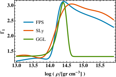
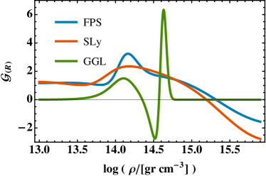
Figure 1: Adiabatic index (left panel) and relativistic fundamental derivative (right panel) as a function of the logarithm of the rest-mass density for the SLy, FPS and GGL EoSs. To obtain a qualitatively similar behaviour of the GGL EoS as in the case of the other two nuclear matter EoSs, we set $\gamma_{0}=4/3$, $\gamma_{1}=3.1$, $\rho_{1}=2.5\times 10^{14}\,$gr cm^-3, $\sigma=0.4$, $\varepsilon=0.01c^{2}$ and $B=\gamma_{0}-1$. We note that, for $B=0$ the adiabatic index is independent of $\varepsilon$ and of $p$.

3.2 The classical and the relativistic fundamental derivatives

In classical fluid dynamics, the convexity of the system is determined by the EoS  (Menikoff & Plohr, 1989; Godlewski & Raviart, 1996) and, more specifically, by the so-called fundamental derivative, ${\mathcal{G}}_{\rm(C)}$ (see its definition - classical - and properties in, e.g., Thompson 1971; Menikoff & Plohr 1989; Guardone et al. 2010)

$${\mathcal{G}}_{\rm(C)}:=-\frac{1}{2}\,V\,\displaystyle{\frac{\displaystyle{\left.\frac{\partial^{2}p}{\partial V^{2}}\right|_{s}}}{\displaystyle{\left.\frac{\partial p}{\partial V}\right|_{s}}}},$$ (27)

where $V:=1/\rho$ is the specific volume and $s$ the specific entropy. Alternative expressions for ${\mathcal{G}}_{\rm(C)}$ are Menikoff & Plohr (1989)

$${\mathcal{G}}_{\rm(C)}=\displaystyle{\frac{1}{2}\left(1+\Gamma_{1}+\left.\frac{\partial\ln\Gamma_{1}}{\partial\ln\rho}\right|_{s}\right),}$$ (28)

and

$${\mathcal{G}}_{\rm(C)}=\displaystyle{1+\left.\frac{\partial\ln{c_{\rm s_{(C)}}}}{\partial\ln{\rho}}\right|_{s}},$$ (29)

The fundamental derivative measures the convexity of the isentropes in the $p-\rho$ plane and if ${\mathcal{G}}_{\rm(C)}>0$ then the isentropes in the $p-\rho$ plane are convex, and the rarefaction waves are expansive.

Analogously to Eq. (28), let us define ${\mathcal{G}}^{+}$

$${\mathcal{G}}^{+}:=\displaystyle{\frac{1}{2}\left\{1+\gamma+\left(\frac{d\ln{\gamma}}{d\ln{\rho}}\right)\right\}}.$$ (30)

From Eq. (29) and for our GGL EoS we obtain:

$${\mathcal{G}}_{\rm(C)}={\mathcal{G}}^{+}+\displaystyle{\frac{\gamma}{2c_{\rm s_{(C)}}^{2}}\left((\gamma\varepsilon+B)\frac{d\ln{\gamma}}{d\ln{\rho}}+\varepsilon\frac{d^{2}\ln{\gamma}}{d(\ln{\rho})^{2}}\right)}$$ (31)

Ibáñez et al. (2013) found that there exist a quantity analogous to the classical fundamental derivative, which they call relativistic fundamental derivative. The following relationship between the classical and relativistic fundamental derivatives holds:

$${\mathcal{G}}_{\rm(R)}={\mathcal{G}}_{\rm(C)}-\frac{3}{2}\,\,c_{\rm s_{(R)}}^{2}$$ (32)

An important consequence of the above result is the following: for a non-convex EoS, there will be a region (in the $p-\rho$ plane) where the thermodynamics is non-convex from the relativistic point of view, i.e., there where ${\mathcal{G}}_{\rm(R)}\leq 0$, but it is convex from the classical point of view ${\mathcal{G}}_{\rm(C)}\geq 0$.

We show in the right panel of Fig. 1 the relativistic fundamental derivative for the GGL EoS as well as for the analytic fits of the FPS and SLy EoSs given in Haensel & Potekhin (2004). We observe that for the chosen parameters of the GGL EoS (see caption of Fig. 1), the relativistic fundamental derivative becomes negative in coincidence with decay post-maximum in $\Gamma_{1}$ (Fig. 1 left panel), signalling the existence of a non-convex thermodynamic region extending between $14.3\lesssim\log{\rho}\lesssim 14.6$. Since the fall-off of $\Gamma_{1}$ in the FPS and SLy EoSs is not so steep, these EoSs do not develop a non-convex region in the same density range as the GGL EoS, yet ${\mathcal{G}}_{\rm(R)}$ drops in the region where $d\Gamma_{1}/d\rho<0$. Eventually, since these two realistic EoS are non-causal at high densities, their relativistic fundamental derivatives become negative.

Noteworthy, the analytic approximations of both the SLy and the FPS EoS smoothes the jump in $\Gamma_{1}$ from $\simeq 1.7$ to $\simeq 2.2$ that occurs in the realistic EoSs they fit. This approximation is also smooth across a small discontinuous drop of $\Gamma_{1}$ at $\rho\simeq 2\times 10^{14}$ gr cm^-3, where muons start to replace a part of the ultrarelativistic electrons. These non-smooth regions of the EoS in terms of $\Gamma_{1}(\rho)$ may potentially yield a negative fundamental derivative (either the classical or the relativistic one). Our simple GGL EoS does not attempt to model the former phenomenology.

3.3 Limits on the values of the parameters of the GGL EoS

In order to restrict the values of some of the parameters in our phenomenological EoS it is convenient to explicitly show the asymptotic values of the sound speed in a couple relevant regimes.

First, we consider the case in which $B=\gamma_{0}-1$. Then

$$\lim_{\rho\rightarrow\infty}p=(\gamma_{0}-1)\rho(1+\varepsilon),$$ (33)

and, therefore, the maximum sound speed allowed by the GGL EoS in this regime is

$$c_{\rm s_{(R)}}^{\rm(max)}=\sqrt{\gamma_{0}-1}.$$ (34)

Consistently, the EoS is causal for values of $\gamma_{0}$ in the range $1\leq\gamma_{0}\leq 2$.

Next, we examine the limiting value of the sound speed for large values of the internal energy (i.e., the ultrarelativistic limit). There, we may define

$$\left(c_{\rm s_{(R)}}^{(+)}\right)^{2}:=\lim_{\varepsilon\rightarrow\infty}c_{\rm s_{(R)}}^{2}=\displaystyle{\gamma-1+\frac{d\ln{\gamma}}{d\ln{\rho}}}=2({\mathcal{G}}^{+}-1).$$ (35)

For the EoS to be causal it is required that

$$0\leq\left(c_{\rm s_{(R)}}^{(+)}\right)^{2}\leq 1,$$ (36)

$$0\leq\left(c_{\rm s_{(R)}}^{\rm(max)}\right)^{2}\leq 1.$$ (37)

Hence, in order to maintain causality, it is necessary that (from Eq. (36))

$$1\leq{\mathcal{G}}^{+}<3/2,$$ (38)

and (from Eqs. (34) and Eq. (37))

$$1\leq\gamma_{0}\leq 2.$$ (39)

Further constraints on the values of the parameters of the GGL EoS can be obtained demanding thermodynamic stability, which needs that $\Gamma_{1}\geq 0$. This condition requires that:

$$\gamma \geq 0$$ (40)

$$\left(c_{\rm s_{(R)}}^{(+)}\right)^{2} \geq -{\displaystyle\frac{B}{\varepsilon}}$$ (41)

Condition (41) is satisfied for all non-negative values of $B$. We note that negative internal energies are allowed by the GLL-EoS if $B>0$, with the only restriction that the pressure they produce must be positive (see, Eq. (20)).

3.4 Typical values

Since the only constraint we have for the value of $B$ is that $B\geq 0$ (Sec. 3.3), we will restrict ourselves to a pair of possibilities, namely, $B=0$, and $B=\gamma_{0}-1$. We point out that in the case $B=0$, if we further set $\gamma_{1}=\gamma_{0}$, the ideal gas EoS with constant adiabatic index $\gamma=\gamma_{0}$ is recovered. As we have already mentioned in Sec. 3, the case $B=\gamma_{0}-1$ yields an effective barotropic behavior of the GGL EoS at high densities.

Within the ranges discussed in Sec. 3.3, we may choose the values of the GGL EoS parameters in order to reproduce the behaviour of, e.g., nuclear matter density. To be more specific, we may tune the parameters of the EoS to reproduce qualitatively the typical regimes found in the framework of core collapse supernovae (CC-SN). With this aim, we set $\gamma_{0}=4/3$ and let $\gamma_{1}$ vary within the range

$$5/3\leq\gamma_{1}\lesssim 1.9.$$ (42)

Likewise, we take $\rho_{1}=1$ in dimensionless units. The latter parameter is a scale factor, whose value in CGS units, and again taking into account the studies of CC-SN during the late stages of the infall epoch and during the bounce epoch, $\rho_{1}\lesssim 10^{15}\,$gr cm^-3 (see, e.g., Janka et al., 2012).

Besides the previous analysis of the GGL EoS, we have carried out an exhaustive analysis of the EOS parameter space. We have payed particular attention to the subspace of EoS parameters for which causality is assured for all values of density and internal specific energy. This subspace depends strongly on the halfwidth of the gaussian sector of the function $\gamma(\rho)$, the general trend (to preserve causality) being that we must include values of $\gamma_{1}$ in the range stated above, if we set larger values of $\sigma$. Our analysis allows us to conclude that suitable values for $\sigma$ (in units of $\rho_{1}$) are $0.60\lesssim\sigma\lesssim 1.10,$ for the values of $\gamma_{1}$ in the range stated in Eq. (42).

4 Relativistic Riemann problems

In this section we aim to set up two Riemann problems that illustrate typical scenarios encountered in relativistic flows. In SRHD, a Riemann problem (RP) is fully specified by providing the states on both sides of an initial surface across which hydrodynamic variables may exhibit discontinuities. We will refer to the uniform states on both sides of the initial discontinuity as “left” and “right” states. Table 1 lists the values of the hydrodynamic variables we take as initial data for two different RPs. The initial states have been carefully chosen to serve as prototypes of different dynamical situations, some of which are genuinely relativistic (i.e., they cannot be found in classical hydrodynamics), inasmuch as some of the initial states fall in a thermodynamic region of non-convexity from the relativistic point of view, but not from the classical point of view (see below).

Table 1: Set up of the three Riemann problems considered in Sec. 4. The first column provides a short text-tag to identify the problem set up. Columns 2-4 (5-7) display the values of the rest-mass density, velocity and pressure left (right) to the initial discontinuity.

Riemann Problem	Acronym	$\rho_{L}$	$v_{L}$	$p_{L}$	$\rho_{R}$	$v_{R}$	$p_{R}$
Blast Wave	BW	$1.0$	$0$	$1000$	$0.125$	$0$	$0.1$
Colliding Slabs	CS	$0.125$	$0.99$	$1.0$	$0.125$	$-0.99$	$1.0$

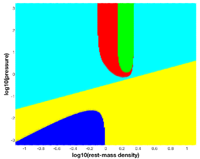
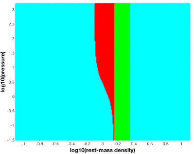
Figure 2: $p-\rho$ diagrams in logarithmic scale of the GGL EoSs defined with parameters in of models EoS1 (left) and EoS2 (right) (see Tab. 2).

In order to understand the nonclassical behavior of the Riemann fan in relativistic hydrodynamics closed with a non-convex EoS, we present two $p-\rho$ diagrams in logarithmic scale of the GGL EoS (Fig. 2) defined with parameters in Tab. 2. We note that with the parameter set EoS3, the GGL EoS reduces to an ideal gas EoS with constant adiabatic index $\gamma=4/3$ which, therefore, does not have any non-convex region. In the following, we will outline the most salient features of the two RPs defined by their initial states (Tab. 1) employing the two parameterizations of the GGL EoS that encompass non-convex regions in the $p-\rho$ (EoS1 and EoS2). We will further compare the non-standard wave pattern that may develop with the latter parameterizations of the EoS with the classical wave patterns that arise when using the EoS3 parameter set.

Table 2: Parameters of the GGL EoS for two prototype thermodynamic situations (EoS1 and EoS2), as well as for a pure ideal gas EoS with constant adiabatic index (EoS3).

Model	$\gamma_{0}$	$\gamma_{1}$	$\sigma$	$B$
EoS1	$4/3$	$1.9$	$1.1$	$\gamma_{0}-1$
EoS2	$4/3$	$1.9$	$1.1$	$0$
EoS3	$4/3$	$4/3$	$1.0$	$0$

The diagram on the left in Fig. 2 corresponds to the $p-\rho$ plane of the GGL EoS employing the parameters of model EoS1 (Tab. 2). Different from the EoS2 and EoS3 models, the EoS1 parameter set features a value $B=\gamma_{0}-1$, which leads to a high-density EoS of barotropic type. We observe five different regions represented with distinct colors. The area in cyan color depicts the region where both ${\mathcal{G}}_{\rm(C)}>0$ and ${\mathcal{G}}_{\rm(R)}>0$. In this region the EoS is convex, both classically and from the relativistic point of view. Hence, a classical wave structure is expected in the Taub adiabat connecting the left and right states. The area in green represents the region where ${\mathcal{G}}_{\rm(C)}<0$ and, consistently, ${\mathcal{G}}_{\rm(R)}<0$. This is a region of non-convexity both in the classical and in the relativistic sense. The section in red corresponds to the case where ${\mathcal{G}}_{\rm(C)}>0$ and ${\mathcal{G}}_{\rm(R)}<0$, which defines a purely relativistic non-convex region. The sector in yellow color responds to the region where the specific internal energy is negative. This region of the parameter space may also arise in realistic nuclear matter EoSs as a result of the (negative) contribution of the interaction potential between different matter constituents, but is typically restricted to a small region around nuclear saturation density (e.g., Engvik et al., 1996; Mansour & Algamoudi, 2012). Finally, the small dark blue area, surrounded by the yellow one, shows the pathological region where the SRHD equations loose hyperbolicity as $c_{\rm s(C)}^{2}<0$.

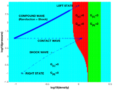
Figure 3: Numerical approximation of the locus of the gas states connecting the left and right states in the $p-\rho$ (EoS2) plane for the BW Riemann problem

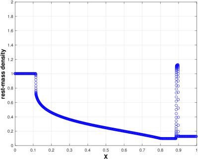
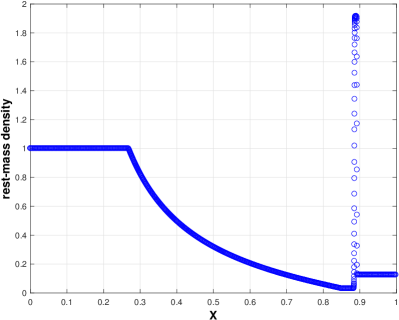
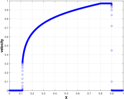
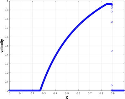
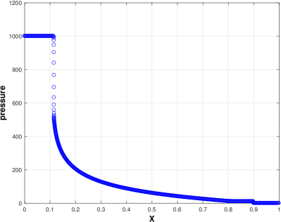
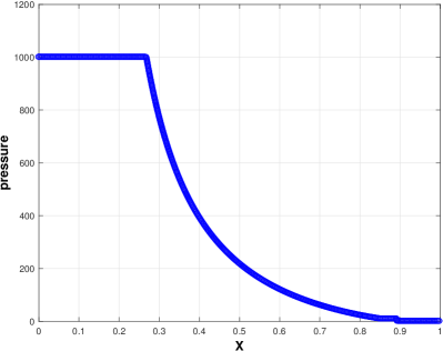
Figure 4: Left column: Rest-mass density (upper left), velocity (middle) and pressure (bottom) of the relativistic blast wave RP set according to Tab. 1 with the GGL EoS and the parameters corresponding to the EoS2 model (Tab. 2). Right column: same as left column but for the relativistic blast wave RP set according to Tab. 1 with the ideal gas EoS corresponding to the EoS3 model.

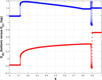
Figure 5: Classical (blue circles) versus relativistic (red asterisks) fundamental derivative profiles of the relativistic blast wave RP set according to Tab. 1 with the GGL EoS and the parameters corresponding to the EoS2 model (Tab. 2).

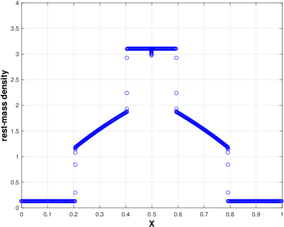
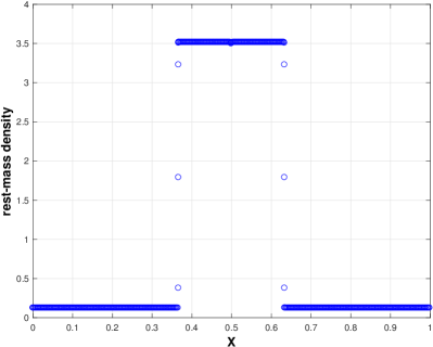
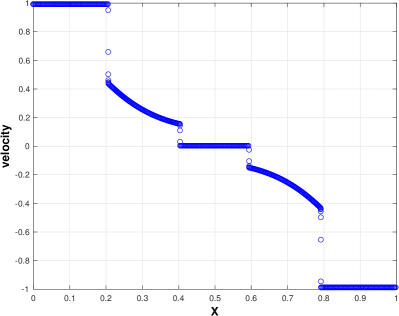
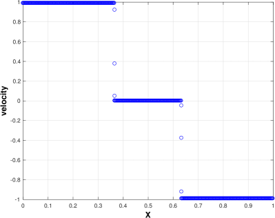
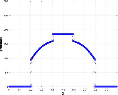
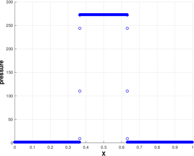
Figure 6: Left column: Rest-mass density (upper left), velocity (middle) and pressure (bottom) of the relativistic colliding slabs RP set according to Tab. 1 with the GGL EoS and the parameters corresponding to the EoS1 model (Tab. 2). Right column: same as left column but for the relativistic colliding slabs RP set according to Tab. 1 with the ideal gas EoS corresponding to the EoS3 model.

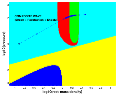
Figure 7: Numerical approximation of the locus of the gas states connecting the left and right states in the $p-\rho$ plane (EoS1) for the CS Riemann problem

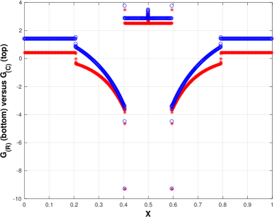
Figure 8: Classical (blue circles) versus relativistic (red asterisks) fundamental derivative profiles of the relativistic colliding slabs RP set according to Tab. 1 with the GGL EoS and the parameters corresponding to the EoS1 model (Tab. 2).

The analogous regions for the GGL EoS setup EoS2 (Tab. 2) are represented in the diagram on the right of Fig. 2. The different colors designate same features as in the diagram on the left. If $B=0$ it is straightforward to prove that ${\mathcal{G}}_{\rm(C)}$ only depends on the density. This feature explains the regular shape of the green vertical band. Another consequence is that both regions of loose of hyperbolicity (dark blue) and negative value of specific internal energy (yellow) are avoided.

We perform numerical simulations by means of a local characteristic approach based on the Marquina Flux Formula for Special Relativistic flows (Martí et al., 1997). In order to resolve the complex wave structure we use a similar strategy as followed in Serna (2009) and Serna & Marquina (2014) to capture composite waves in magnetohydrodynamics. The numerical scheme uses two linearizations at each side of the interface computing the numerical fluxes through a Lax-Friedrichs approach ensuring stability and entropy satisfying solution. We implement high order accuracy in space following the Shu-Osher flux formulation (Shu & Osher, 1989) by using a third order reconstruction procedure based on hyperbolas (Marquina, 1994). High order accuracy in time is achieved by a third order TVD Runge-Kutta time stepping procedure (Shu & Osher, 1989).

Unless stated otherwise, in the following, we will show the solution of the RPs at a time $t=0.4$ after the initial discontinuity begins to break up ($t=0$). The exact value of the final time to represent the solution is physically irrelevant since the solution of the RP is self-similar in SRHD and planar geometry. The value we take here is adequate to show the details of the Riemann wave pattern in various figures of this section. The solution is computed with $12800$ uniform grid points and a CFL factor $C_{\mathrm{CFL}}=0.4$.

We first compare the evolution of a blast wave with the GLL-EoS and parameters of the sets EoS2 and EoS3 (Tab. 2). The initial data in Tab. 1 (BW) corresponds to a relativistic strong blast wave such that the left state belongs to the red region (the purely relativistic non-convex region) in the diagram on the right in Fig. 2. The right state belongs to the cyan region, (the pure classical convex region). Fig. 3 shows the numerical approximation of the path connecting the left and right states in the $p-\rho$ plane for the RP at hand. The profiles of the wave structure in rest-mass density, velocity and pressure are shown in the left panels of Fig. 4. These exhibit a path connecting both states, consisting of a shock wave propagating to the right and a rarefaction wave attached to a shock wave (composite wave), separated by a contact wave. Figure 5 shows the profiles of the classical and relativistic fundamental derivatives. The latter shows that the left wave breaks into two pieces at the point where the relativistic fundamental derivative changes sign, forming a composite wave (shock plus rarefaction). We note that should we chose the left state in the classical non-convex region (green region in Fig. 3), the resulting wave pattern would have been qualitative similar. However, this RP example is genuinely relativistic and shows that beyond the classical region of convexity loss, relativistic effects my drive a non-convex dynamics.

For comparison, we provide in the right panels of Fig. 4 the evolution of the same initial data as in the BW case (Tab. 1), but for an ideal gas EoS with $\gamma=4/3$, corresponding to the tag EoS3 in Tab. 2. The profiles of the wave structure in density, velocity and pressure show the classical wave structure of a relativistic blast wave, an expansive rarefaction starting at the left state, a contact and a shock wave.

We have not included a variant of the relativistic blast wave problem with the EoS1 parameter set. The reason is that the Taub adiabat joining the initial states for this test (Tab. 1) does not cross over any non-convex region. Hence, the resulting wave pattern is qualitatively equal to the one generated with the EoS3 parameter set of the GGL EoS.

The left panels of Fig. 6 exhibit the evolution at time $t=0.4$ of two relativistic colliding slabs with GGL EoS parameters of the set EoS1. The initial data in Tab. 1 consist of two streams of gas hitting each other with opposite and equal speeds of $0.99$. Both the density and the pressure of the left and right states of the RP are uniform and identical. Their values have been chosen in such a way that the left and right states belong to the cyan region of Fig. 2 (right panel) and are located at the same point. Therefore, both states fall in a region where the EoS is convex, but as we observe, the Taub adiabat joining them transits over the non-convex realm of the EoS, as shown in the diagram in Fig. 7, resulting into a striking dynamics. The solution is symmetric with respect to the center of the domain because the initial velocities are prescribed with the same magnitude and opposite sign in order to hit the two gases at the center. The wave structure consists of two composite waves traveling from the center in opposite directions. Each composite wave consist of three pieces, two shock waves connected through a rarefaction wave. The profile of the classical and relativistic fundamental derivatives in Fig. 8 reveals the region of negative values where the anomalous wave structure appears. Employing an ideal EoS (EoS3 in Tab. 2) the initial discontinuity breaks up into just two symmetric shock waves traveling towards the boundary of the domain at constant velocity (right panels of Fig. 6). Should we use the EoS2 parameter set for the GGL EoS, we would have obtained a qualitatively equal wave pattern than obtained with the EoS3 parameter set, since the Taub adiabat does not pierce the non-convex regions of the $p-\rho$-plane for the initial states of the relativistic colliding slabs RP.

5 Discussion and conclusions

The aim of this paper is to show the rich and complex dynamics that an EoS with non-convex regions in the $p-\rho$ plane may develop as a result of genuinely relativistic effects, without a classical counterpart. To best serve our purposes, we have introduced a phenomenological EoS, the GLL-EoS, which depends on five parameters that can be restricted heeding to causality and thermodynamic stability constraints. This EoS shall be regarded as a toy-model with which we may mimic realistic (and far more complex) EoS of practical use in the realm of Relativistic Hydrodynamics. Actually, causality and thermodynamic stability restrictions provide an ample playground for the variation of the GLL-EoS parameters. We exploit this freedom to calibrate the parameters so that our simple closure reproduces some qualitative behaviors found in microphysical EoSs of matter around and above nuclear saturation density. In particular, the non-monotonic dependence of the sound speed (equivalently of the adiabatic index) with the rest-mass density. Certainly, the non-monotonic dependence of $\Gamma_{1}$ on $\rho$ can also be found in many other contexts within Astrophysics (e.g., in problems involving partially ionized plasma) and elsewhere (e.g., in material processing), and it may not always result in a non-convex thermodynamics. The latter depends on whether this lack of monotonicity translates into a negative fundamental derivative.

The dynamic effects of a non-convex EoS gleam when discontinuities are set in the fluid or result from its non-linear evolution. Studying the breakup of an initial discontinuity in the flow is a simple yet effective way of exploring the aforementioned dynamics. Fortunately, there exist a physically sound and mathematically elegant set up whereby the evolution of discontinuous and piecewise uniform initial data can be computed, namely, solving a RP. Thus, we have carefully set up the initial data of prototype RPs in which, either one of the states corresponds to a non-convex relativistic thermodynamical state, or the Taub adiabat joining the initial data pierces through a region of relativistic non-convexity of the EoS. In the former case, we tune the physical state to be convex in a classical sense (i.e., the classical fundamental derivative evaluated on the initial data is positive). As expected, non-convex dynamics can develop structures such as rarefaction shocks, compound waves, etc., which are in clear contrast to the wave structure that a convex EoS generates.

The interest of this study is not purely academic and may have far reaching implications (beyond the scope of this publication) in various fields of Astrophysics (e.g., stellar core collapse of massive stars, the merger of compact binaries), Cosmology (e.g., in the evolution of the Early Universe), Nuclear Physics (e.g., the collision of heavy ions), etc. Precisely, the impact that a non-convex EoS may have on the dynamics of stellar core collapse we will be the subject of a subsequent paper (Ibáñez et al., 2017). There, we will show that non-convex dynamics may leave an imprint on the gravitational wave signature of the system, specially if the non-magnetized core rotates fast and differentially, which could be observed by future gravitational wave detectors or suitable upgrades of the existing ones. We however note that the presence of strong (dynamically relevant) magnetic fields in a collapsing stellar core may counterbalance the effects of a non-convex EoS, both from the mathematical point of view and physics-wise. Mathematically, Serna & Marquina (2014) in the classical MHD case and Ibáñez et al. (2015) for relativistic MHD showed that the fundamental derivative for either Newtonian or relativistic, magnetized fluids adds a positively defined term to the relativistic fundamental derivative. This term grows with increasing magnetic field strength. Hence, strong magnetic fields reduce the ranges of thermodynamic states where the fundamental derivative may be negative, i.e., where the system loses its convexity. Reinforcing this point, Serna & Marquina (2014) show numerical examples in which a strong enough magnetic field may revert the non-convexity effects induced by two different non-convex EoS. From the physical point of view, strong magnetic fields break the rotation of massive stellar cores (e.g. Yamada & Sawai, 2004; Heger et al., 2005; Obergaulinger & Aloy, 2017) and, therefore, weaken the gravitational wave signature of the system (Kotake et al., 2004; Obergaulinger et al., 2006). These facts highlight the need of a deeper numerical study of the potential physical effects that non-convex EoS have in the context of magneto-rotational core collapse.

References

- Aloy et al. (1999) Aloy M. A., Ibáñez J. M., Martí J. M., Müller E., 1999, ApJS, 122, 151
- Anile (2005) Anile A. M., 2005, Relativistic Fluids and Magneto-fluids
- Aoki et al. (2006) Aoki Y., Endrődi G., Fodor Z., Katz S. D., Szabó K. K., 2006, Nature, 443, 675
- Asplund et al. (1999) Asplund M., Nordlund Å., Trampedach R., Stein R. F., 1999, A&A, 346, L17
- Banik et al. (2014) Banik S., Hempel M., Bandyopadhyay D., 2014, ApJS, 214, 22
- Baumgarte et al. (2000) Baumgarte T. W., Shapiro S. L., Shibata M., 2000, ApJ, 528, L29
- Bauswein et al. (2014) Bauswein A., Stergioulas N., Janka H.-T., 2014, Phys. Rev. D, 90, 023002
- Bazavov et al. (2014) Bazavov A., et al., 2014, Phys. Rev. D, 90, 094503
- Bedaque & Steiner (2015) Bedaque P., Steiner A. W., 2015, Physical Review Letters, 114, 031103
- Borsányi et al. (2014) Borsányi S., Fodor Z., Hoelbling C., Katz S. D., Krieg S., Szabó K. K., 2014, Physics Letters B, 730, 99
- Borsanyi et al. (2016) Borsanyi S., et al., 2016, Nature, 539, 69
- Chabanat et al. (1997) Chabanat E., Bonche P., Haensel P., Meyer J., Schaeffer R., 1997, Nuclear Physics A, 627, 710
- Chabanat et al. (1998) Chabanat E., Bonche P., Haensel P., Meyer J., Schaeffer R., 1998, Nuclear Physics A, 635, 231
- Chandrasekhar (1939) Chandrasekhar S., 1939, An introduction to the study of stellar structure. The University of Chicago press
- Cinnella & Congedo (2007) Cinnella P., Congedo P. M., 2007, Journal of Fluid Mechanics, 580, 179
- Cinnella et al. (2011) Cinnella P., Marco Congedo P., Pediroda V., Parussini L., 2011, Physics of Fluids, 23, 116101
- Clark et al. (2011) Clark P. C., Glover S. C. O., Klessen R. S., Bromm V., 2011, ApJ, 727, 110
- Collet et al. (2007) Collet R., Asplund M., Trampedach R., 2007, A&A, 469, 687
- D’Angelo & Bodenheimer (2013) D’Angelo G., Bodenheimer P., 2013, ApJ, 778, 77
- Engvik et al. (1996) Engvik L., Osnes E., Hjorth-Jensen M., Bao G., Ostgaard E., 1996, ApJ, 469, 794
- Flower et al. (2003) Flower D. R., Bourlot J. L., Des Forêts G. P., Cabrit S., 2003, Monthly Notices of the Royal Astronomical Society, 341, 70
- Font et al. (1994) Font J. A., Ibanez J. M., Marquina A., Marti J. M., 1994, A&A, 282, 304
- Glover & Abel (2008) Glover S. C. O., Abel T., 2008, MNRAS, 388, 1627
- Godlewski & Raviart (1996) Godlewski E., Raviart P., 1996, Numerical Approximation of Hyperbolic Systems of Conservation Laws. Springer
- Greif et al. (2011) Greif T. H., Springel V., White S. D. M., Glover S. C. O., Clark P. C., Smith R. J., Klessen R. S., Bromm V., 2011, ApJ, 737, 75
- Guardone et al. (2010) Guardone A., Zamfirescu C., Colonna P., 2010, Journal of Fluid Mechanics, 642, 127
- Haensel & Potekhin (2004) Haensel P., Potekhin A. Y., 2004, A&A, 428, 191
- Heger et al. (2005) Heger A., Woosley S. E., Spruit H. C., 2005, ApJ, 626, 350
- Hempel et al. (2012) Hempel M., Fischer T., Schaffner-Bielich J., Liebendörfer M., 2012, ApJ, 748, 70
- Hotokezaka et al. (2011) Hotokezaka K., Kyutoku K., Okawa H., Shibata M., Kiuchi K., 2011, Phys. Rev. D, 83, 124008
- Ibáñez et al. (2012) Ibáñez J. M., Cordero-Carrión I., Miralles J. A., 2012, Classical and Quantum Gravity, 29, 157001
- Ibáñez et al. (2013) Ibáñez J. M., Cordero-Carrión I., Martí J. M., Miralles J. A., 2013, Classical and Quantum Gravity, 30, 057002
- Ibáñez et al. (2015) Ibáñez J.-M., Cordero-Carrión I., Aloy M.-Á., Martí J.-M., Miralles J.-A., 2015, Classical and Quantum Gravity, 32, 095007
- Ibáñez et al. (2017) Ibáñez J.-M., Sanchis-Gual N., Font J. A., Aloy M.-Á., Serna S., Marquina A., 2017, MNRAS(sumitted)
- Janka et al. (2012) Janka H.-T., Hanke F., Hüdepohl L., Marek A., Müller B., Obergaulinger M., 2012, Progress of Theoretical and Experimental Physics, 2012, 01A309
- Jappsen et al. (2005) Jappsen A.-K., Klessen R. S., Larson R. B., Li Y., Mac Low M.-M., 2005, A&A, 435, 611
- Kippenhahn & Weigert (1990) Kippenhahn R., Weigert A., 1990, Stellar structure and evolution. Astronomy and astrophysics library, Springer, https://books.google.es/books?id=G4jvAAAAMAAJ
- Kiuchi et al. (2009) Kiuchi K., Sekiguchi Y., Shibata M., Taniguchi K., 2009, Phys. Rev. D, 80, 064037
- Kotake et al. (2004) Kotake K., Yamada S., Sato K., Sumiyoshi K., Ono H., Suzuki H., 2004, Phys. Rev. D, 69, 124004
- Laine & Schröder (2006) Laine M., Schröder Y., 2006, Phys. Rev. D, 73, 085009
- Li et al. (2003) Li Y., Klessen R. S., Mac Low M.-M., 2003, ApJ, 592, 975
- Luzum & Romatschke (2008) Luzum M., Romatschke P., 2008, Phys. Rev. C, 78, 034915
- Mansour & Algamoudi (2012) Mansour H. M. M., Algamoudi A. M. A., 2012, Physics of Atomic Nuclei, 75, 430
- Marquina (1994) Marquina A., 1994, SIAM J. Sci. Comp., 15, 892
- Marquina et al. (2017) Marquina A., Serna S., Ibáñez J.-M., 2017, (in preparation)
- Martí et al. (1997) Martí J. M., Müller E., Font JA. andIbañez J. M., Marquina A., 1997, J. Comp. Phys, 479, 151
- Menikoff (2007) Menikoff R., 2007, Empirical Equations of State for solids. Springer Berlin Heidelberg
- Menikoff & Plohr (1989) Menikoff R., Plohr B. J., 1989, Reviews of Modern Physics, 61, 75
- Muñoz & Kamionkowski (2015) Muñoz J. B., Kamionkowski M., 2015, Phys. Rev. D, 91, 043521
- Nonaka & Bass (2007) Nonaka C., Bass S. A., 2007, Phys. Rev. C, 75, 014902
- Obergaulinger & Aloy (2017) Obergaulinger M., Aloy M. Á., 2017, MNRAS, 469, L43
- Obergaulinger et al. (2006) Obergaulinger M., Aloy M. A., Müller E., 2006, A&A, 450, 1107
- Pandharipande & Ravenhall (1989) Pandharipande V. R., Ravenhall D. G., 1989, in Soyeur M., Flocard H., Tamain B., Porneuf M., eds, NATO Advanced Science Institutes (ASI) Series B Vol. 205, NATO Advanced Science Institutes (ASI) Series B. p. 103
- Rauscher et al. (2002) Rauscher T., Heger A., Hoffman R. D., Woosley S. E., 2002, ApJ, 576, 323
- Rezzolla & Zanotti (2013) Rezzolla L., Zanotti O., 2013, Relativistic Hydrodynamics. Oxford University Press
- Roth & Kasen (2015) Roth N., Kasen D., 2015, ApJS, 217, 9
- Serna (2009) Serna S., 2009, J. Comp. Phys, 228, 4232
- Serna & Marquina (2014) Serna S., Marquina A., 2014, Physics of Fluids, 26, 016101
- Shen et al. (2011) Shen G., Horowitz C. J., O’Connor E., 2011, Phys. Rev. C, 83, 065808
- Shu & Osher (1989) Shu C., Osher S., 1989, J. Comput. Phys., 83, 32
- Spaans & Silk (2000) Spaans M., Silk J., 2000, ApJ, 538, 115
- Takami et al. (2014) Takami K., Rezzolla L., Baiotti L., 2014, Physical Review Letters, 113, 091104
- Thompson (1971) Thompson P. A., 1971, Physics of Fluids, 14, 1843
- Thompson & Lambrakis (1973) Thompson P., Lambrakis K., 1973, J. Fluid Mechanics, 60, 187
- Vaidya et al. (2015) Vaidya B., Mignone A., Bodo G., Massaglia S., 2015, A&A, 580, A110
- Yamada & Sawai (2004) Yamada S., Sawai H., 2004, ApJ, 608, 907
- Yoshida et al. (2006) Yoshida N., Omukai K., Hernquist L., Abel T., 2006, ApJ, 652, 6