Bands and gaps in Nekrasov partition function

A. Gorsky^2,3, A. Milekhin^1,3,4 and N. Sopenko^1,2,3 

¹ Institute of Theoretical and Experimental Physics, B.Cheryomushkinskaya 25, Moscow 117218, Russia

² Moscow Institute of Physics and Technology, Dolgoprudny 141700, Russia

³ Institute for Information Transmission Problems of Russian Academy of Science, B. Karetnyi 19, Moscow 127051, Russia

⁴ Department of Physics, Princeton University, Princeton, NJ 08544, USA

gorsky@itep.ru, milekhin@itep.ru, niksopenko@gmail.com

Abstract

We discuss the effective twisted superpotentials of 2d $\mathcal{N}=(2,2)$ theories arising upon the reduction of 4d $\mathcal{N}=2$ gauge theories on the $\Omega$-deformed cigar-like geometry. We explain field-theoretic origins of the gaps in the spectrum in the corresponding quantum mechanical (QM) systems. We find local 2d descriptions of the physics near these gaps by resumming the non-perturbative part of the twisted superpotential and discuss arising wall-crossing phenomena. The interpretation of the associated phenomena in the classical Liouville theory and in the scattering of two heavy states in $AdS_{3}$ gravity is suggested. Some comments concerning a possible interpretation of the band structure in QM in terms of the Schwinger monopole-pair production in 4d are presented.

1 Introduction

The Seiberg-Witten (SW) solution of $\mathcal{N}=2$ SYM theories [1] provides an impressive example of how the summation over the non-perturbative configurations in the non-integrable quantum field theory amounts for the powerful information concerning the low-energy effective action and the spectrum of the stable particles. The combination of the educated physical guesses and the analytic tools allowed to treat the strong coupling regime exactly. In the case of pure $SU(2)$ theory it was discovered that the naive classical singularity where the $W$-boson becomes massless split into two singular points, where the monopole and the dyon become massless instead, enclosed by the curve of marginal stability (CMS) within which the W-boson becomes unstable and no longer exists in the spectrum. If $\mathcal{N}=2$ SUSY is softly broken down to $\mathcal{N}=1$ SUSY the singular points of the Coulomb moduli space correspond to the vacuum states of the $\mathcal{N}=1$ SYM theory.

The Seiberg-Witten result was reproduced microscopically by Nekrasov [2, 3] by considering the theory in the $\Omega$-background $\mathbf{C}^{2}_{\epsilon_{1},\epsilon_{2}}$ that provides the IR regularization by localizing the integrals over the instanton moduli spaces on a set of isolated fixed points. The partition function is expressed as a sum of the contributions from each of these points. The Seiberg-Witten prepotential, which defines the low-energy effective action, can be extracted from the Nekrasov partition function as the leading term of the logarithm of the partition function in the limit $\epsilon_{1},\epsilon_{2}\rightarrow 0$.

The information contained in the Seiberg-Witten solution can be usefully packed in the pair of integrable Hamiltonian systems. First, the Seiberg-Witten curves which encode the information about the low-energy actions were identified with the spectral curves of the classical holomorphic integrable many-body systems [4, 5, 6, 7, 8, 9]. The type of the integrable many-body system is in one-to-one correspondence with the matter content of the $\mathcal{N}=2$ SYM theory. The SW variables $a,a_{D}$ were identified with the action and the dual action in the corresponding integrable system. The prepotential on the other hand was naturally identified in terms of the second Whitham integrable system [4, 10] that is the semiclassical limit of the (1+1) dimensional KdV or Toda field theory. In the Whitham theory the variables $a,a_{D}$ form the symplectic pair while the prepotential $\mathcal{F}$ plays the role of the action variable which can be immediately seen from the relation $a_{D}=\frac{\partial\mathcal{F}}{\partial a}$ which is the analogue of the relation $p=\partial S/\partial q$ in the Hamiltonian mechanics. The time in the Whitham dynamics was identified with the logarithm of the instanton counting parameter $\log\Lambda$. The coordinates in the first integrable system were identified with the positions of the defect branes in some internal coordinate [8, 9].

The next step in this correspondence was made in [11, 12, 13]. It was argued that by turning on an $\Omega$-background with only one non-zero parameter $\epsilon_{1}$ the many-body type integrable system gets quantized with a Planck constant $\hbar=\epsilon_{1}$. The Yang-Yang function (YY) of this system, which provides the Bethe Ansatz equations for a particular quantization, coincides with the effective twisted superpotential of the effective two-dimensional $\mathcal{N}=(2,2)$ theory that appears upon the reduction on the plane with $\Omega$-background turned on with the appropriate choice of the boundary conditions at the boundary of this plane, while the quantum states are identified with the vacua of this theory. The effective twisted superpotential arises as the leading term in the logarithm of the partition function in the Nekrasov-Shatashvili (NS) limit $\epsilon=\epsilon_{2}\to 0$. A more precise description of this two dimensional theory was given in [14].

An interesting feature that appears in quantum many-body integrable systems is the presence of exponentially small in $\hbar$ gaps between the energy bands for a particular type of quantization. For example, for pure $U(2)$ gauge theory one of the quantizations leads to the famous Mathieu spectral problem which gives the spectrum of a particle in a periodic cosine potential. This gap between the bands has a transparent physical interpretation in this quantum mechanical problem and appears due to quantum reflection over the barrier. However, it looks rather mysterious from the gauge theoretic point of view. The four-dimensional $W$-boson leads to an infinite tower of two-dimensional particles in the effective theory upon the reduction, and a quick inspection shows that some of this particles naively become massless precisely at those values of the Coulomb parameters, for which the splitting phenomenon appears, undermining the validity of the low-energy effective description. These special values of the Coulomb parameters also appear as poles in the instanton part of the superpotential. For each splitting point there are infinitely many poles of all orders in the instanton series.

The goal of the present paper is to describe the physics near this loci. What we have found is that after a proper resummation of the non-perturbative part and after combining it with the perturbative contribution the naive pole singularities in the superpotential transform into the cuts. The fate of the corresponding two-dimensional $W$-boson mode is rather similar to the fate of the four-dimensional $W$-boson in the undeformed theory: it decays into lighter particles before becoming massless on the curve of marginal stability that encloses the cut. In our case this lighter particles are solitons which interpolate between the vacua corresponding to split quantum states.

Let us note that the procedure of trans-series resummation that we actually use is known in the mathematical literature as the trans-asymptotic matching [15]. It concerns the reordering of the summation of trans-series near the naive poles. The procedure has been successfully applied for the Painleve I and Painleve II equations [15] and in the physical context it was applied for the trans-series for the gradient expansion of the hydrodynamical equations in [16]. It was argued that the leading term of the resummed trans-series obeys a nonlinear equation which is universal while the next terms of the expansion of the resummed trans-series can be derived via the recursion relation from the leading term. We shall focus in this study on the leading term in the resummed trans-series for the twisted superpotential which locally describes the low-energy physics near the cuts when $\hbar$ is large.

Remarkably, the twisted superpotential for this local description has a rather familiar form. For pure $U(2)$ gauge theory it coincides with the superpotential of the sigma model on $\mathbf{CP}^{1}$ with the twisted mass which is proportional to the ”distance” $\sim(2a-\hbar)$ from the naive singularities at $2a=\hbar$, and the two vacua of this sigma model correspond to split levels. This identification allows us to read out the BPS spectrum of light particles of the effective theory near the cuts, since the BPS spectrum for $\mathbf{CP}^{1}$-model was derived long time ago [17, 18]. We also make a non-trivial check that in the local description of $U(N)$ gauge theory one has the sigma model on a flag variety, with the flag type determined by the level splitting pattern.

The AGT correspondence [19] relates the Nekrasov partition function with the conformal blocks in the Liouville theory. The NS limit in the gauge theory corresponds to the classical limit on the Liouville side. Hence it is natural to ask what kind of non-perturbative phenomena in Liouville theory the non-perturbative phenomena in QM correspond to. It is known that (see, for instance [20, 21]) that the twisted superpotential of $SU(2)$ SYM with adjoint matter coincides with the classical one-point torus conformal block in the Liouville theory while $SU(2)$ SYM with fundamental matter coincides with the classical 4-point spherical conformal block. It is useful to map the classical torus 1-point conformal block to the particular 4-point spherical conformal block [22, 23] hence all $SU(2)$ examples can be considered on equal footing.

The 2-point torus classical conformal block involving the $\Psi_{2,1}$ degenerate operator obeys the Lame equations [24]. The Mathieu equation can be derived in a proper limit from Lame equation and its solution was identified with the irregular conformal block involving coherent Gaiotto state [25]. Therefore we shall argue that naive poles in intermediate dimensions in classical 4-point conformal block disappear upon the trans-series resummation.

The classical Liouville conformal block by $AdS_{3}/CFT_{2}$ holographic correspondence (see [26] for a review) is lifted to a particular process in $AdS_{3}$ bulk gravity. It was identified with the on-shell action evaluated on the geodesic network in 3d gravity [27, 28, 29]. The effects of operator insertions at the boundary depend on the behavior of their dimensions in the classical limit. If the operator is heavy, that is its conformal dimension is proportional to the central charge, it deforms the bulk and amounts to BTZ black hole or conical defect depending on the value of the classical conformal dimension. The light operators correspond to the geodesic motion in the bulk perturbed by the heavy operators [27, 30, 31, 32, 33]. The accessory parameter in the Liouville theory which is related to the energy in the QM problems corresponds to the conserved Killing momentum on the gravity side [27, 28, 29]. Since we have explained the mechanism of the disappearance of the naive poles in the classical Liouville conformal blocks, the natural question concerns the meaning of the corresponding non-perturbative phenomena in $AdS_{3}$ gravity.

It turns out that all four operators in the spherical conformal block are heavy and the intermediate dimension is related to the heavy operator as well. The naive poles correspond to the points where the intermediate state becomes degenerate and in the limit of the large Planck constant(in QM sense) we are focusing on the ”OPE limit” in the conformal block. Since all operators are heavy we are dealing with the scattering of the degrees of freedom which deform the bulk gravity. Not much is known about the scattering S-matrix in $AdS_{3}$-gravity however some non-perturbative phenomena have been considered for instance in [34, 35]. In particular it was shown that there is the exponentially suppressed process of the black hole formation in collision of two particles representing conical defects [35].

Therefore the gravity problem at hand involves the extremal BTZ BH and particles yielding conical singularities. Using the map between the classical conformal block and on-shall gravity action for the scattering process we claim that the poles in the scattering amplitude as the function of the intermediate dimension disappears upon the resummation of trans-series and the CMS around the naive pole emerges. The CMS can be considered as the curve on the plane of the complex intermediate dimension at fixed time or the curve at the complex time plane at fixed intermediate dimension. This suggests that probably the transition between early times and late times proceeds through a kind of CMS.

There is an interesting similarity of our case with the low-energy monopole scattering [36]. That process can be described as the geodesic motion at the 2-monopole moduli space which has a non-trivial Atiyah-Hitchin metric - the non-perturbative generalization of the Taub–NUT metric. There are specific geodesics on the monopole moduli space which result in the excitation of the motion along $S^{1}$ direction of the monopole moduli space. Physically it means that the monopoles become dyons in the scattering process. This happens because the initial angular momentum of the monopoles gets transformed into the angular momentum of the electromagnetic field in the collision process. In the physical space the process can be described by the exchange of the light $W$-boson between two heavy monopoles.

The $AdS_{3}$ gravity can be described via $SL(2,\mathbb{R})\times SL(2,\mathbb{R})$ Chern-Simons theory [37, 38]. Hence we are dealing with the moduli space of flat connections and the corresponding Teichmuller spaces(which are analogues of the monopole moduli space for the monopole scattering). The twisted superpotential is the action for the Whitham dynamics which on the other hand corresponds to the geodesic motion on the Teichmuller space similar to the monopole case. It is natural to conjecture that similar to the monopole case the motion along the compact dimension of the moduli space can be excited in the process.

It was conjectured in [39] that some kind of the Schwinger-type phenomena takes place in SYM which corresponds to the bounce-induced phenomena in QM however no mechanism has been found. We shall present some arguments that the non-perturbative monopole pair production in the external graviphoton field is relevant for the bounce induced phenomena in the QM. We shall also comment on the relation of the Schwinger-like picture to the representation of the Nekrasov partition function via the Myers effect in the external graviphoton field.

There were several previous studies addressing the issue of singularities in the effective twisted superpotential. In [40] the resummation procedure that we use in this paper was performed for finite-gap $\mathcal{N}=2^{*}$ $U(2)$ gauge theory. In [41] the partition functions of half-BPS surface defects near the corresponding locus were studied. It is necessary to mention [42] where the Mathieu equation has been obtained in the mini-superspace approximation in the sine-Gordon model on a cylinder. The absence of the naive singularity in the plane of quasi-momentum in the sine-Gordon model has clear a physical interpretation. The quasi-momentum is related to the effective constant electric field in the fermionic representation and the emergence of the cut instead of the logarithmic singularities is associated with the Schwinger-type pair production in the external electric field.

The paper is organized as follows. In section 2 we review some facts concerning the Nekrasov partition function and Bethe/gauge correspondence. In section 3 we discuss the low-energy description of the effective $\mathcal{N}=(2,2)$ two-dimensional theory. We perform the resummation of non-perturbative contribution and show that the naive singularities of the superpotential in the Coulomb parameters get transformed into the cuts. We extract the local superpotentials near these cuts and discuss their physical implications. In section 4 the interpretation of this phenomena in the classical Liouville theory and its holographic dual is discussed. Some conjectures concerning the possible relation with the monopole-pair production in the $\Omega$-background are presented in section 5. The considerations in sections 4 and 5 are more qualitative however they suggest useful physical insights and analogies. The results and the open questions are collected in Conclusion.

2 Generalities on the Bethe/gauge correspondence

In this section we review the Bethe/gauge correspondence [43, 44, 45, 11, 12, 13] to set up the conventions and formulate the problem. Throughout the paper we only discuss the case of theories with a single $U(N)$ gauge group.

2.1 Instanton partition function

First, let us recall the definition of the Nekrasov partition function [2, 3] of a four dimensional gauge theory in the $\Omega$-background $\mathbf{C}^{2}_{\epsilon,\hbar}$.

Let $\mathbf{a}$ denote a set of complex scalars which parametrize the moduli space of vacua, $\mathbf{m}$ is set of masses for fundamental matter multiplets and $\Lambda^{2N}=\exp(2\pi i\tau)$ is a generated mass scale that counts instantons.

The full Nekrasov partition function consists of perturbative and non-perturbative contributions

$$Z(\mathbf{a},\mathbf{m},\Lambda;\epsilon,\hbar)=Z^{pert.}(\mathbf{a},\mathbf{m},\Lambda;\epsilon,\hbar)\times Z^{inst.}(\mathbf{a},\mathbf{m},\Lambda;\epsilon,\hbar)$$ (1)

The non-perturbative part of the partition function is obtained by the equivariant localization on the instanton moduli space and is defined as follows. Let

$$\mathcal{V}_{\lambda}=\sum_{i=1}^{N}\sum_{(r,s)\in\lambda_{i}}e^{a_{i}+(r-1)\epsilon+(s-1)\hbar},\,\,\,\,\,\,\,\mathcal{W}=\sum_{i=1}^{N}e^{a_{i}},\,\,\,\,\,\mathcal{M}=\sum_{i=1}^{N_{f}}e^{m_{i}}$$ (2)

$$\mathcal{T}_{\lambda}=-\mathcal{M}\mathcal{V}_{\lambda}^{*}+\mathcal{W}\mathcal{V}_{\lambda}^{*}+e^{\epsilon+\hbar}\mathcal{V}_{\lambda}\mathcal{W}^{*}-(1-e^{\epsilon})(1-e^{\hbar})\mathcal{V}_{\lambda}\mathcal{V}_{\lambda}^{*}$$ (3)

which appear as the characters of the natural bundles on the instanton moduli space at a fixed point, parametrized by a set $\{\lambda_{i}\}$ of $N$ Young diagrams. The star-operation inverts all weights of a character:

$$\biggl{(}\sum_{a}e^{w_{a}}\biggr{)}^{*}=\sum_{a}e^{-w_{a}}$$ (4)

The instanton partition function can be written as

$$Z^{inst.}(\mathbf{a},\mathbf{m},\Lambda;\epsilon,\hbar)=\sum_{\{\lambda\}}\Lambda^{2N|\lambda|}e(\mathcal{T}_{\lambda})$$ (5)

where

$$e(\sum_{a}e^{w_{a}}-\sum_{b}e^{w_{b}})=\frac{\prod_{b}w_{b}}{\prod_{a}w_{a}}$$ (6)

is a symbol that converts the sum of characters into the product of weights.

The perturbative part is more subtle due to ambiguity of the boundary conditions at infinity [46]. It can be written as

$$Z^{pert.}(\mathbf{a},\mathbf{m},\Lambda;\epsilon,\hbar)=\Lambda^{-\frac{N}{\epsilon\hbar}\sum_{i=1}^{N}a_{i}^{2}}e\biggl{(}\frac{e^{\epsilon+\hbar}(\mathcal{M}\mathcal{W}^{*}-\mathcal{W}\mathcal{W}^{*})}{(1-e^{\epsilon})(1-e^{\hbar})}\biggr{)}$$ (7)

but since the character now has infinitely many terms a proper regularization is needed. Physically the first multiplier comes from the tree level contribution, while the first and the second terms in the character come from the one-loop contribution of the matter multiplets and $W$-bosons, respectively.

Note that the perturbative contribution does depend on the instanton counting parameter since it defines the running coupling constant $\tau$.

2.2 Nekrasov-Shatashvili limit

The low-energy description of undeformed four dimensional gauge theory is characterized by the prepotential, which can be obtained as the limit of the deformed partition function

$$\mathcal{F}(\mathbf{a},\mathbf{m},\Lambda)=\lim_{\epsilon,\hbar\to 0}\epsilon\,\hbar\log Z(\mathbf{a},\mathbf{m},\Lambda;\epsilon,\hbar)$$ (8)

It is known that it is related to some classical algebraic integrable system [4, 6]. In particular the moduli space of vacua of the theory coincides with the base of the Liouville fibration of this system. The underlying integrable system for a large class of quiver gauge theories was found in [47].

In [13] a refinement of the correspondence with integrable systems was proposed. It was argued that the effective two dimensional theory, which appears in the limit $\epsilon\to 0$, is related to the corresponding quantized algebraic integrable system, and $\hbar$ plays the role of the quantization parameter.

More precisely we can consider a four dimensional gauge theory on $\mathbf{C}\times\mathbf{D}_{\hbar}$ where $\mathbf{D}_{\hbar}$ is the cigar-like geometry of [14] with the $\Omega$-deformation turned on. With an appropriate twist this geometry breaks half of the supersymmetries. Upon choosing the boundary conditions on $\mathbf{C}\times\partial\mathbf{D}_{\hbar}=\mathbf{C}\times S^{1}$ which preserve the remaining supersymmetries, we can reduce our theory to a two-dimensional $\mathcal{N}=(2,2)$ theory on $\mathbf{C}$, the low energy description of which is characterized by the effective twisted superpotential

$$\mathcal{W}(\mathbf{a},\mathbf{m},\Lambda;\hbar)=\lim_{\epsilon\to 0}\epsilon\log{Z(\mathbf{a},\mathbf{m},\Lambda;\hbar)}$$ (9)

For the perturbative contribution we have

$$\mathcal{W}^{pert.}(\mathbf{a},\mathbf{m},\Lambda;\hbar)=\lim_{\epsilon\to 0}\epsilon\log Z^{pert.}(\mathbf{a},\mathbf{m},\Lambda;\epsilon,\hbar)=\\ -\frac{1}{2\hbar}\log\biggl{(}\frac{\Lambda^{2N}}{\hbar^{2N}}\biggr{)}\sum_{i=1}^{N}a_{i}^{2}+\sum_{i,j=1}^{N}\varpi_{\hbar}(a_{i}-a_{j})-\sum_{i=1}^{N}\sum_{a=1}^{N_{f}}\varpi_{\hbar}(a_{i}-m_{a})$$ (10)

where $\varpi_{\hbar}(x)$ obeys

$$\frac{d}{dx}\varpi_{\hbar}(x)=\log\Gamma\biggl{(}1+\frac{x}{\hbar}\biggr{)}=const.-\sum_{n=1}^{\infty}\log\biggl{(}\frac{x+n\hbar}{\hbar}\biggr{)}$$ (11)

The one-loop contribution $\varpi_{\hbar}(m)$ has a simple intuitive explanation as a contribution of infinite number of angular momentum modes with mass parameters $(m+n\hbar)$ for $n$-th mode into the effective twisted superpotential, which are chiral multiplets in the effective two dimensional theory. Indeed, after integrating out a single chiral multiplet we get

$$\Delta\mathcal{W}_{n}=-(m+n\hbar)\biggl{[}\log\biggl{(}\frac{m+n\hbar}{\hbar}\biggl{)}-1\biggr{]}$$ (12)

and after summing over $n$ we get $\varpi_{\hbar}(m)$.

In principle, if no accidental cancellations happen, the effective two dimensional theory has infinitely many local degrees of freedom, which have different angular momentum along $\mathbf{D}$ weighted with the massive parameter $\hbar$.

There are two natural boundary conditions [14] which require

$$\operatorname{Type}A:\,\,\,\,\,\,\,\,\,\frac{a^{D}_{i}}{\hbar}=\frac{\partial\mathcal{W}(\mathbf{a},\mathbf{m},\Lambda;\hbar)}{\partial a_{i}}\in\mathbf{Z}$$ (13)

$$\operatorname{Type}B:\,\,\,\,\,\,\,\,\frac{a_{i}}{\hbar}\in\mathbf{Z}+\frac{\theta_{i}}{2\pi},\,\,\,\,\theta\in[0,2\pi)$$ (14)

Type $A$ corresponds to Neumann-type boundary condition for gauge fields leading to a dynamical vector multiplet in two dimensions. On the contrary type $B$ corresponds to Dirichlet boundary conditions, fixing the holonomy along the boundary of the cigar parametrized by $\theta_{i}$ and freezing gauge degrees of freedom. The choice of this boundary conditions specifies the quantization of an algebraic integrable system.

The Bethe/gauge correspondence states that the vacua of the effective two dimensional theory are in one-to-one correspondence with the eigenstates of the Hamiltonians of the quantum integrable system. Moreover, the expectation values of the topologically protected chiral observables, which are traces of the adjoint scalars in a vector multiplet $\operatorname{Tr}\mathbf{\Phi}^{k}$ of a four dimensional theory, coincide with the eigenvalues of the Hamiltonians $\mathcal{H}_{k}$ on this states:

$$\langle vac|\mathcal{H}_{k}|vac\rangle\longleftrightarrow\langle\operatorname{Tr}\mathbf{\Phi}^{k}\rangle_{vac.}$$ (15)

The simplest example of such correspondence for purely four dimensional gauge theory is the periodic $A_{N-1}$ Toda chain.

2.3 Pure $U(N)$ and the periodic Toda chain

The (complexified) periodic Toda chain is a one-dimensional system of $N$ non-relativistic particles interacting with the following potential

$$V(x_{1},...,x_{N})=\Lambda^{2}\sum_{i=1}^{N}e^{x_{i}-x_{i+1}},\,\,\,\,\,\,\,x_{N+1}=x_{1}$$

where the coordinates $x_{i}\in\mathbf{C}/(2\pi\mathbf{Z})$ while the momenta $p_{i}\in\mathbf{C}$. The set of classical Hamiltonians $\{H_{i}\}$ is conveniently encoded in the spectral curve equation

$$\det(x-L(w))=x^{N}+H_{1}x^{N-1}+H_{2}x^{N-2}+...+H_{N}-\Lambda^{N}(z+z^{-1})=0$$ (16)

where $L(z)$ is a Lax operator

$$L(z)=\left(\begin{matrix}p_{1}&\Lambda^{2}e^{x_{1}-x_{2}}&0&\dots&\dots&\Lambda^{N}z^{-1}\\ 1&p_{2}&\Lambda^{2}e^{x_{2}-x_{3}}&\dots&\dots&0\\ 0&1&p_{3}&\Lambda^{2}e^{x_{3}-x_{4}}&\dots&0\\ 0&\dots&\dots&\dots&\dots&0\\ 0&\dots&\dots&\dots&p_{N-1}&\Lambda^{2}e^{x_{N-1}-x_{n}}\\ \Lambda^{2-N}e^{x_{N}-x_{1}}z&0&\dots&0&1&p_{N}\\ \end{matrix}\right)$$ (17)

The first two Hamiltonians are

$$H_{1}=-\sum_{i=1}^{N}p_{i}$$ (18)

$$H_{2}=-\frac{1}{2}\sum_{i\neq j}p_{i}p_{j}+V(x_{1},...,x_{N})$$ (19)

As is well known the underlying 4d $\mathcal{N}=2$ gauge theory for this system is the pure $U(N)$ theory. In particular its Seiberg-Witten curve coincides with the spectral curve of the integrable system [4, 5].

We are interested in the quantization of this system. The Hamiltonians and the momenta are now promoted to differential operators, acting on wave functions $\psi(x_{1},...,x_{N})$ with $p_{i}=\hbar\partial_{i}$. There are two natural quantizations, corresponding to type $A$ and type $B$ boundary conditions [13]. Type $A$ quantization corresponds to $x_{i}\in\mathbf{R}$ and $\psi(x_{1}-\bar{x},...,x_{N}-\bar{x})\in L^{2}(\mathbf{R}^{N-1})$ where $\bar{x}=\sum_{i}^{N}x_{i}/N$ is the center of mass mode, which decouples in a trivial way. This condition leads to discrete unambiguous spectrum that corresponds to the set of vacua in the gauge theory, provided that the type $A$ boundary condition $a_{D}/\hbar\in\mathbf{Z}$ is satisfied.

In this paper we are interested in type $B$ quantization that corresponds to $x_{i}\in i\mathbf{R}/2\pi\mathbf{Z}$ and quasi-periodic non-singular wave functions

$$\psi(x_{1},...,x_{a}+2\pi i,...,x_{N})=e^{i\theta_{a}}\psi(x_{1},...,x_{N})$$ (20)

The quasi-periodicity parameters $\theta_{a}\in[0,2\pi)$ are also known as Bloch-phases. In the special case of $N=2$, after the decoupling of the center of mass mode, the equation on the wave function coincided with Mathieu equation

$$-\hbar^{2}\psi^{\prime\prime}(x)+8\Lambda^{2}\cos(2x)\psi(x)=8u\psi(x)$$ (21)

where $u=\frac{1}{4}\langle\operatorname{Tr}\mathbf{\Phi}^{2}\rangle$. For real $\Lambda$ and $\hbar$ it describes a particle moving in a periodic cosine potential. At fixed $\theta$-parameters the spectrum is discrete. However as we vary them the spectrum consists of peculiar structure of bands and gaps. In particular for small $\Lambda$ and when we sit near the edge of some band, the spectrum has exponentially small in $\sim 1/\hbar$ splitting of the eigenvalues. More precisely if $\theta_{1}=...=\theta_{k_{1}};\theta_{k_{1}+1}=...=\theta_{k_{2}};...;\theta_{k_{m}+1}=...=\theta_{k_{N}}$ and are all integers, then instead of naive $\frac{N!}{k_{1}!k_{2}!...k_{N}!}$-fold degeneracy as for $\Lambda=0$ we have non-degenerate spectrum due to quantum reflection on the potential.

This second type of quantization appears to be more mysterious from the gauge theory point of view. When all $\theta$-parameters are zero $a_{a}/\hbar$ are forced to be equal to integer, and when $a_{ab}/\hbar\in\mathbf{Z}\setminus\{0\}$ some perturbative $W$-boson modes naively become massless that is clear from the logarithmic singularities in their perturbative contribution into the effective twisted superpotential. Thus naively the effective description has to break down at this locus, as was pointed out in [41]. One of the main purposes of the present paper is to resolve this puzzling issue.

3 Effective two-dimensional field theory

In this section we are interested in the physics of the effective two-dimensional $\mathcal{N}=(2,2)$ gauge theory, which appears upon the reduction of $\mathcal{N}=2$ four-dimensional gauge theory in the $\Omega$-background as was described in the previous section. Our main example will be the simplest non-trivial case of pure $U(2)$ gauge theory, though we will also comment on a few generalizations.

3.1 Pure $U(2)$ theory

In this case the superpotential $\mathcal{W}(a,\Lambda;\hbar)$ depends on a single complex parameter $a$ parametrizing vacua. The superpotential has the following expansion:

$$\mathcal{W}(a,\Lambda;\hbar)=\mathcal{W}^{pert.}(a,\Lambda;\hbar)-\hbar\,F(\nu,q)$$ (22)

$$F(\nu,q)=\sum_{k=1}^{\infty}F_{k}(\nu)q^{2k}$$ (23)

where we have introduced dimensionless variables $\nu$ and $q$:

$$\nu={2a\over\hbar},\,\,\,\,\,\,\,\,\,q=\frac{\Lambda^{2}}{\hbar^{2}}$$ (24)

The perturbative part $\mathcal{W}^{pert.}$ of the superpotential is

$$\mathcal{W}^{pert.}(a,\Lambda;\hbar)=-\frac{2a^{2}}{\hbar}\log\biggl{(}\frac{\Lambda^{2}}{\hbar^{2}}\biggr{)}+\varpi_{\hbar}(2a)+\varpi_{\hbar}(-2a)$$ (25)

and the first few terms for $F_{k}(s)$ are

$$\sum_{k=1}^{\infty}F_{k}(\nu)q^{2k}=\frac{2}{\nu^{2}-1}q^{2}+\frac{5\nu^{2}+7}{(\nu^{2}-1)^{3}(\nu^{2}-4)}q^{4}+\frac{16\left(9\nu^{4}+58\nu^{2}+29\right)}{3\left(\nu^{2}-1\right)^{5}\left(\nu^{2}-4\right)(\nu^{2}-9)}q^{6}\\ +\frac{1469\nu^{10}+9144\nu^{8}-140354\nu^{6}+64228\nu^{4}+827565\nu^{2}+274748}{2\left(\nu^{2}-4\right)^{3}\left(\nu^{2}-1\right)^{7}\left(\nu^{2}-9\right)\left(\nu^{2}-16\right)}q^{8}+...$$ (26)

The characteristic feature that we observe for all $F_{k}(s)$ is that they all have poles at non-zero integers $s=n$ for $-k\leq n\leq k$. However, as we will see shortly they are just artifacts of the expansion in small $q$.

There is a single independent chiral trace operator $u=\frac{1}{4}\langle\operatorname{Tr}\mathbf{\Phi}^{2}\rangle$. It is related to the superpotential via quantum version of Matone relation [49], [50], [51]

$$u=-\frac{\hbar}{8}\Lambda\frac{\partial\mathcal{W}(a,\Lambda;\hbar)}{\partial\Lambda}$$ (27)

Below we will often need the monopole mass $|a_{D}^{M}|$ which is in our normalization reads as:

$$a_{D}^{M}=i\cfrac{\hbar}{4\pi}\cfrac{\partial\mathcal{W}(a,\Lambda;\hbar)}{\partial a}$$ (28)

For large $a$ such that $a\gg\Lambda$ and $a\gg\hbar$ instanton corrections are suppressed and one can find using eqs. (25) and (11) that:

$$a_{D}^{M}=i\cfrac{2a}{\pi}\log{\cfrac{2a}{\Lambda}}+O(a)$$ (29)

since in this limit $\varpi_{\hbar}(x)=\frac{x^{2}}{2\hbar}\log{\frac{x}{\hbar}}+O(x)$

3.1.1 Mathieu equation

As was discussed in the previous section, the finding of the expectation values of chiral trace operator in different vacua of the effective two dimensional theory for type $B$ boundary conditions is equivalent to finding of the spectrum of the Mathieu equation

$$-\psi^{\prime\prime}(x)+8q\cos(2x)\psi(x)=\frac{8u}{\hbar^{2}}\psi(x)$$ (30)

with quasi-periodic boundary conditions $\psi(x+\pi)=e^{\pi i\nu}\psi(x)$. In particular, for real $\Lambda$ and $\hbar$ the spectrum has an alternate set of bands and gaps with exponentially small band widths in “low” spectrum when $u\approx-\Lambda^{2}$ and exponentially small gap widths in “high” spectrum when $u\gg\Lambda^{2}$.

Since $\pi\nu$ is a Bloch phase the function $u(q,\nu)$ has period $2$ in $\nu$ on the real axes. However, this periodicity is not manifest in the expansion obtained by inserting (26) into the Matone relation (27). For example, when we change $\nu$ along $[0,2]$ and are supposed to return back we meet the singularity at $\nu=1$ in each term of the expansion. A possible resolution is that instead of these naive poles the function $u(\nu,q)$ has branch cuts as shown on the figure (1) with the identification of cuts near $\nu=n$ and $\nu=-n$ to make it 2 periodic, and when we expand it in $q$ we loose this branch cut structure and obtain poles. The latter happens if the widths of this cuts vanish as $q$ goes to 0. The identification of $\nu=n$ and $\nu=-n$ is natural since $\nu$ is proportional to a Coulomb parameter $a$ which transforms under Weyl symmetry as $a\to-a$.

Figure 1: This picture shows the branch cut structure of the function $u(q,\nu)$. Each cut near $\nu=n$ is identified with the cut near $\nu=-n$. As the result of this identification we obtain an infinite-genus surface.

3.1.2 Resummation

To obtain a good expansion of $F(\nu,q)$ near the cuts we use the same trick as in [40] and reorganize the expansion in $q$ in the following way

$$F(\nu,q)=\sum_{n>0}\sum_{k=1}^{\infty}\biggl{[}g_{k}^{(n)}\biggl{(}\frac{q^{n}}{n-\nu}\biggr{)}+g_{k}^{(n)}\biggl{(}\frac{q^{n}}{n+\nu}\biggr{)}\biggr{]}q^{2k-2+n}$$ (31)

where $g_{k}^{(n)}(z)=\mathcal{O}(z)$ and we have introduced variable $z$:

$$z=\frac{q^{n}}{n-\nu}$$ (32)

What is physical meaning of this resummation? From more technical point of view, it corresponds to resumming separately the leading singularity from each instanton sector(function $g_{1}^{(n)}$) then the subleading singularity (function $g_{2}^{(n)}$) and so on. As we will see shortly, $\log{q^{n}}$ plays the role of 2d FI parameter, whereas $n-\nu$ is proportional to the mass of light W-boson mode. The combination $\log{q^{n}}-\log\left(n-\nu\right)$ is exactly 2d effective FI parameter once we integrate out a particle of mass $n-\nu$. Therefore this expansion reorganizes the 4d instanton expansion into a double expansion in terms of 2d effective vortices and 4d instantons.

By comparing the first few terms in the expansions of (31) and $(\ref{eq:oldF})$ in $q$ we expect that $g_{k}^{(n)}$ have the following form

$$g^{(n)}_{1}(z)=\frac{\log\left(\frac{1}{2}+\sqrt{\frac{1}{4}+\frac{z^{2}}{\zeta_{n}^{2}}}\right)+1-\sqrt{1+\frac{4z^{2}}{\zeta_{n}^{2}}}}{z}$$ (33)

for $k=1$ and

$$g_{k}^{(n)}(z)=\frac{\left(1+\frac{4z^{2}}{\zeta_{n}^{2}}\right)^{\frac{5}{2}-k}Q_{2k-3}\left(z^{2}\right)+P_{k-1}\left(z^{2}\right)}{z^{2k-1}}$$ (34)

for $k>1$, where $\zeta_{n}=n!(n-1)!$ and $P_{m}(w)$, $Q_{m}(w)$ are some polynomials of degree $m$, specific for each $n$ and $k$. Using this ansatz and $g_{k}^{(n)}(z)=\mathcal{O}(z)$, one can compute $P$ and $Q$ polynomials which appear $g_{k}^{(n)}(z)$ for any given $n$ and $k$ by expanding the Nekrasov partition function up to the corresponding order. We present the first few $g_{k}^{(n)}$ functions in the Appendix A.

Once we have reorganized the expansion in this form, we capture the branch cut structure provided that we identify the cuts near $n$ and $-n$ that was proposed in the previous subsection. In particular, we can write down a perturbative in $q$ expressions for band/gap edges for $\nu\approx n$ using the quantum Matone relation, which coincide with the known expressions (see e.g. [39])

$$\begin{split}u_{0}={\hbar^{2}\over 8}\left(-q+\frac{7}{4}q^{3}-\frac{58}{9}q^{5}+\frac{68687}{2304}q^{7}+\ldots\right)\\ u_{1}^{-}={\hbar^{2}\over 8}\left(1-4q-2q^{2}+q^{3}-\frac{1}{6}q^{4}-\frac{11}{36}q^{5}+\ldots\right)\\ u_{1}^{+}={\hbar^{2}\over 8}\left(1+4q-2q^{2}-q^{3}-\frac{1}{6}q^{4}+\frac{11}{36}q^{5}+\ldots\right)\\ \dots{}\end{split}$$ (35)

3.1.3 Local model

Now let us try to explain the physical implications of the appearance of the branch cuts instead of the naive poles. Let us build a simplified local model near the first pole $m=(\hbar-2a)\to 0$ in the limit of very large $\Omega$-background $\hbar\gg\Lambda$ or $q\ll 1$. Naively, when $\hbar$ and $a$ are very large, the instanton corrections are switched off and only the perturbative part contributes

$$\mathcal{W}^{pert.}(a,\Lambda;\hbar)\approx-m\biggl{[}\log\biggl{(}\frac{m}{\hbar}\biggl{)}-1\biggr{]}+const.$$ (36)

which is nothing else but the contribution of a first W-boson angular momentum mode, that naively becomes massless at $2a=\hbar$. However, looking at the reorganized expansion for the non-perturbative part we see that the first leading term has the same order in $q$ as the perturbative one, and

$$\mathcal{W}(a,\Lambda;\hbar)\approx-m\biggl{[}\log\biggl{(}\frac{m}{\hbar}\biggl{)}-1\biggr{]}-q\hbar\,g^{(1)}_{1}\biggl{(}\frac{q}{1-\nu}\biggr{)}+const.\\ =-m\log\biggl{(}\frac{m+\sqrt{m^{2}+\frac{4\Lambda^{4}}{\hbar^{2}}}}{2\hbar}\biggr{)}+\sqrt{m^{2}+\frac{4\Lambda^{4}}{\hbar^{2}}}+const.$$ (37)

It is instructive to look at the mirror description of this system. Consider

$$\mathcal{W}=m(Y-t_{eff.})+e^{-Y}+(\Lambda^{4}/\hbar^{2})e^{Y}.$$ (38)

where $t_{eff.}=\log(\hbar^{-1})$. If we integrate out the field $Y$ we return back to (37). What we obtain is the mirror description of chiral multiplet deformed by $(\Lambda^{4}/\hbar^{2})e^{Y}$ operator.

Now we can try to give a physical interpretation of this additional term. As is well known $e^{-Y}$ is related to the appearance of vortex configurations in the mirror description. Similar $e^{Y}$ is related to the appearance of vortex configurations with the opposite charge. In the case of free chiral multiplet such term doesn’t appear since it has wrong quantum numbers. However in our case the parameter $(\Lambda^{4}/\hbar^{2})$ also carries quantum numbers and in combination with $e^{Y}$ allows for the terms of the form $(\Lambda^{4}/\hbar^{2})^{n}e^{(2n-1)Y}$. Since we work in the first non-zero order in $(\Lambda^{4}/\hbar^{2})$ we have only the term $(\Lambda^{4}/\hbar^{2})e^{Y}$. The appearance of $\Lambda^{4}$ which measures the instanton charge suggests that the configuration that has a negative vortex charge also carries the instanton charge and it is this charge that allows for negative vortex numbers.

Curiously similar deformation appears in a local model of a theory of a chiral doublet surface defect in a pure $SU(2)$ gauge theory, which is obtained by coupling 2d $\mathcal{N}=(2,2)$ chiral doublet theory, living on $\mathbf{C}\subset\mathbf{C}^{2}$, to 4d $\mathcal{N}=2$ $SU(2)$ theory via weakly gauging of a global $SU(2)$ symmetry of the doublet [52]. In that case the effective twisted superpotential for the defect, that takes into account bulk effects, is

$$\mathcal{W}=-\langle\operatorname{Tr}(m+\Phi)\bigl{(}\log(m+\Phi)-1\bigr{)}\rangle_{4d}$$ (39)

where $m$ is the twisted mass parameter for the diagonal $U(1)$ symmetry of the doublet and $\Phi$ is the bulk vector multiplet scalar. The bulk averaging $\langle...\rangle_{4d}$ can be done using the resolvent of [3]

$$R(x)=\operatorname{Tr}\frac{1}{x+\Phi}=\frac{2x}{\sqrt{(x^{2}-2u)^{2}-4\Lambda^{2}}}$$ (40)

which gives

$$-\partial_{m}\mathcal{W}=\log{\Lambda^{2}}+\operatorname{arccosh}\frac{m^{2}-2u}{2\Lambda^{2}}$$ (41)

and for large $m^{2}$ and $2u\approx a^{2}$ close to $2u\approx m^{2}$

$$-\partial_{m}\mathcal{W}\approx\log{\Lambda^{2}}+\operatorname{arccosh}\frac{m-a}{\Lambda^{2}/a}.$$ (42)

A mirror description of this region is

$$\mathcal{W}=(m-a)Y+e^{-Y}-(\Lambda^{4}/4a^{2})e^{Y}$$ (43)

and similarly to our case the perturbative 2d description of the chiral doublet is deformed by $(\Lambda^{4}/(4a^{2}))e^{Y}$ which appears due to instantons in the bulk. In this situation the source of this term has a simple interpretation in the brane construction of this defect [53] and appears in the microscopic derivation of the superpotential [54, 55, 56].

3.1.4 Wall-crossing near the cut

Now we can answer what happens with the $W$-boson mode that naively becomes massless near $\nu\approx n$. It has to disappear from the BPS spectrum and thus decays into other BPS objects on some curve of marginal stability.

Let us again consider the mirror superpotential for our local model (38) near the first pole. The vacuum values of $Y$ are

$$Y^{(\pm,n)}=\log\biggl{(}\frac{-m\pm\sqrt{m^{2}+\frac{4\Lambda^{4}}{\hbar^{2}}}}{\frac{2\Lambda^{4}}{\hbar^{2}}}\biggr{)}+2\pi in,\,\,\,\,\,n\in\mathbb{Z}$$ (44)

where $2\pi in$ appears due to the multivaluedness of the logarithm function. In the original global description this vacua correspond to two split states near $\nu\approx 1$ and lie in the two neighboring bands. It is easy to find the degeneracies of BPS particles, connecting different vacua using the methods of [57], [58]. However one can simply notice that our local superpotential coincides with the well known mirror description of $\mathbf{CP}^{1}$ sigma model with a twisted mass, for which the BPS spectrum was already analyzed in [17]. Indeed, the twisted superpotential for $\mathbf{CP}^{1}$ has the form (e.g. [59])

$$\mathcal{W}_{\mathbf{CP}^{1}}(t,m)=\Sigma(Y_{1}+Y_{2}-2t)+\frac{m}{2}(Y_{1}-Y_{2})+e^{-Y_{1}}+e^{-Y_{2}}$$ (45)

where $t$ and $m$ are the Kähler parameter of $\mathbf{CP}^{1}$ and the twisted mass, correspondingly. After integrating out the fields $\Sigma$ and $Y_{2}$ we obtain

$$\mathcal{W}_{\mathbf{CP}^{1}}(t,m)=m(Y_{1}-t)+e^{-Y_{1}}+e^{-2t}e^{Y_{1}}$$ (46)

that gives us (38) up to a constant if $e^{-t}=\Lambda^{2}/\hbar$.

Translating [17] into our notations, the result for the BPS spectrum is the following. In the region of large enough $m$ there is a single state that connects $Y^{(\pm,n)}$ and $Y^{(\pm,n+1)}$ and a tower of single states which interpolate between $Y^{(+,n)}$ and $Y^{(-,n+k)}$. The former one has a mass $|m|$ and corresponds to a W-boson mode while the latter corresponds to solitons, coupled to $k$ W-boson modes. On the other hand in the region of small $m$ there are only two single states, connecting vacua $Y^{(-,n)}$ and $Y^{{(+,n)}}$. The masses of this two particles are

$$M_{sol.}=\biggl{|}\frac{1}{2\pi}\frac{\Lambda^{2}}{\hbar}\biggl{[}4\sqrt{1+\frac{\hbar^{2}m^{2}}{4\Lambda^{4}}}+\frac{\hbar m}{\Lambda^{2}}\log\biggl{(}\frac{m\hbar-\sqrt{4\Lambda^{2}+m^{2}\hbar^{2}}}{m\hbar+\sqrt{4\Lambda^{2}+m^{2}\hbar^{2}}}\biggr{)}\biggl{]}\biggr{|}.$$ (47)

and in the $m\rightarrow 0$ limit

$$M_{sol.}=\biggl{|}\frac{2}{\pi}\frac{\Lambda^{2}}{\hbar}\biggr{|}$$ (48)

On the curve of marginal stability $|m|=2M_{sol.}$ all states of the large $m$ region including W-boson mode decay into this two particles.

Note that the electric charge of W-boson in the 4d theory is 2 and the electric charge of all other BPS particles is integer in the units of W-boson charge. On the other hand in the effective 2d theory the solitons both have charge 1. Thus this solitons do not simply come from the modes of other BPS particles but appear only due to the generated superpotential.

Remark. One may ask why we do not obtain in the spectrum of 2d BPS particles the modes of 4d particles with non-zero magnetic charge. At least in the undeformed theory in the region of large $u$ we expect the whole tower of dyons, but the effective twisted superpotential doesn’t have monodromies associated with this particles. The resolution of this puzzle lies in the boundary condition that we impose. Indeed as was shown in [14] type $B$ quantization leads to Dirichlet boundary condition for gauge fields. As the result the flux of magnetic field through $\mathbf{S}^{1}_{\infty}\times\partial\mathbf{D}_{\hbar}$ where $\mathbf{S}^{1}_{\infty}$ is the circle at infinity of $\mathbf{C}$ has to be zero and that select only the particles with zero magnetic charge. In contrast the same reasoning allows only for electrically neutral particles for type $A$ quantization.

Though this analysis was done for the first gap $2a\to\hbar$, it is straightforward to do the same local analysis near all other gaps for small $q$. We again obtain a pair of solitons with masses

$$M_{n}=\frac{2\hbar}{\pi}\frac{1}{n!(n-1)!}\biggl{(}\frac{\Lambda^{2}}{\hbar^{2}}\biggr{)}^{n}$$ (49)

and $n$-th $W$-boson mode decays into this solitons near the corresponding gap. Note that for large $n$ using eq. (29) we have:

$$M_{n}\sim\exp\biggl{(}-\frac{2\pi|a^{M}_{D}|}{\hbar}\biggr{)}$$ (50)

However, our analysis is restricted to the limit of large $\Omega$-background $\Lambda/\hbar\ll 1$ and to a set of light BPS particles. In particular it doesn’t tell us anything about the strong coupling region $u\sim\Lambda^{2}$. It would be interesting to explore this region and the global structure of the BPS spectrum.

3.2 Pure $U(N)$ theory

So far we have considered the case of $U(2)$ gauge theory and have seen, that $\mathcal{N}=(2,2)$ $\mathbf{CP}^{1}$ model appears in the local description ”near the gap”. One may ask how it generalizes to the case of $U(N)$ theories, e.g. for $N$-particle periodic Toda system. In that case we already have different types of singularities parametrized by a set of integers $(k_{1},...,k_{l})$ such that $k_{1}+...+k_{l}=N$, as was described in section 2. This singularities appear at $a_{1}=...=a_{k_{1}}$, $a_{k_{1}+1}=...=a_{k_{2}}$, … , $a_{k_{l-1}+1}=...=a_{k_{l}}$ and $(a_{a}-a_{b})\in\mathbf{Z}\setminus\{0\}$ otherwise. The degeneracy of this singularities is $\frac{N!}{k_{1}!...k_{l}!}$.

A natural candidate for the local description near the singularity is a $\mathcal{N}=(2,2)$ sigma model on the space $\operatorname{Fl}_{(k_{1},...,k_{l})}$ of flags $\mathbf{C}^{k_{1}}\subset\mathbf{C}^{k_{1}+k_{2}}\subset...\subset\mathbf{C}^{N}$. As a trivial check the degeneracy of the singularity coincides with the number of vacua in this sigma model, and the number possible deformations of Coulomb parameters $\mathbf{a}$ coincides with the number of possible twisted mass parameters. However, in this sigma model we can also vary $l-1$ Kähler parameters $\{t_{s}\}$, the option that we don’t have in the local model. So the Kähler parameters have to be specified in terms of $\Lambda$ and $\hbar$.

The effective twisted superpotential for this sigma model can be obtained via describing it as a low-energy limit of a gauged linear sigma model. The set of fields is encoded in a quiver shown on the figure (2).

Figure 2: A quiver diagram for the gauged linear sigma model that is described by the sigma model on a flag variety.

Each circle-node corresponds to a vector multiplet for a gauge group $U(n_{s})$ where $n_{s}=k_{1}+...k_{s}$ and each arrow corresponds to a chiral multiplet in the bifundamental representation. The last square-node corresponds to a global $U(N)$ symmetry with parameters $m_{1},...,m_{N}$, which correspond to the twisted mass parameters of the sigma model. The Kähler parameters comes from the Fayet-Iliopoulos parameters $t_{s}$ on each node. The effective superpotential has the following form

$$\mathcal{W}(\mathbf{\sigma},\mathbf{m},\mathbf{t})=\sum_{s=1}^{l-1}\sum_{i=1}^{n_{s}}t_{s}\sigma^{(s)}_{i}-\sum_{i=1}^{N}\sum_{j=1}^{n_{l-1}}(m_{i}-\sigma^{(l-1)}_{j})\log\frac{(m_{i}-\sigma^{(l-1)}_{j})}{e}\\ -\sum_{s=1}^{l-2}\sum_{i=1}^{n_{s}}\sum_{j=1}^{n_{s+1}}(\sigma^{(s+1)}_{i}-\sigma^{(s)}_{j})\log\frac{(\sigma^{(s+1)}_{i}-\sigma^{(s)}_{j})}{e}\\ +\sum_{s=1}^{l-1}\sum_{i\neq j}^{n_{s}}(\sigma^{(s)}_{i}-\sigma^{(s)}_{j})\log\frac{(\sigma^{(s)}_{i}-\sigma^{(s)}_{j})}{e}\\$$ (51)

where $\sigma^{(s)}_{i}$ are the Coulomb parameters in the vector multiplet of the $s$-th node. After minimizing it with respect to $\mathbf{\sigma}$ by solving vacuum equations

$$\exp\frac{\partial\mathcal{W}(\mathbf{\sigma},\mathbf{m},\mathbf{t})}{\partial\sigma_{i}}\biggl{|}_{\sigma_{*}}=1$$ (52)

we obtain the effective twisted superpotential for our sigma model $\mathcal{W}_{SM}(\mathbf{m},\mathbf{t})=\mathcal{W}(\sigma_{*},\mathbf{m},\mathbf{t})$.

We expect that after proper identification of $\mathbf{t}$ in terms of $\Lambda$ and $\hbar$ the result of the resummation of the instanton partition function near the corresponding singularity $\tilde{\mathbf{a}}$ will be given by $\mathcal{W}_{SM}(\mathbf{m},\mathbf{t})$ with $m_{i}=\tilde{a}_{i}-a_{i}$ . In the next subsection we make make a non-trivial check of this proposal for the case of the full flag variety $\operatorname{Fl}_{(1,....,1)}$ near the singularity $\tilde{a}_{i}=(i-1)\hbar$.

Our strategy is the following. We turn on the second $\Omega$-background parameter $\epsilon$ and consider the fully deformed Nekrasov partition function. From the point of view of the effective two dimensional theory it corresponds to introducing a two-dimensional $\Omega$-background. The resulting partition function is the vortex partition function [60, 61, 62, 63] for this effective theory. We will see that in the limit $\hbar\to\infty$ near the gap this partition function reduces to the vortex partition function of the desired sigma model.

3.2.1 Full flag sigma model from Nekrasov partition function

Let us consider the Nekrasov partition function of pure $U(N)$ gauge theory with $a_{s}=(s-1)\hbar-m_{s}$ in the limit $\hbar\to\infty$ with $z=\Lambda^{2N}/\hbar^{2N-2}$ fixed. Looking at the character of the tangent space at a fixed point $\lambda$

$$\mathcal{T}^{pure}_{\lambda}=\mathcal{W}\mathcal{V}_{\lambda}^{*}+e^{\epsilon+\hbar}\mathcal{V}_{\lambda}\mathcal{W}^{*}-(1-e^{\epsilon})(1-e^{\hbar})\mathcal{V}_{\lambda}\mathcal{V}_{\lambda}^{*}$$ (53)

one can see that only a subset of diagrams with the condition that $\lambda_{s}$ has at most $(N-s)$ rows has a non-vanishing contribution. Indeed, if this condition is not satisfied then too many terms terms in the character contain $\hbar$ in the exponent that leads to a $o(\hbar^{2-2N})$ contribution after applying $e$-symbol.

Let us introduce $k^{(s)}_{i}=\lambda_{i,s-i+1}$, $\sigma^{(s)}_{i}=m_{i}-\epsilon k^{(s)}_{i}$ and

$$z_{s}=\frac{(-1)^{N}z}{s!(s-1)!(N-s)!(N-s-1)!}$$

Then the Nekrasov partition function takes the following form

$$Z^{inst.}=\sum_{k^{(s)}_{i}\geq 0}\biggl{(}\prod_{s=1}^{N-1}z_{s}^{\sum_{i}k^{(s)}_{i}}\times\prod_{s=1}^{N-1}\prod_{i=1}^{s}\prod_{j=1}^{s+1}\frac{1}{(\sigma^{(s+1)}_{j}-\sigma^{(s)}_{i};-\epsilon)_{k^{(s)}_{i}-k^{(s+1)}_{j}}}\\ \times\prod_{s=1}^{N-1}\prod_{i\neq j}^{N}(\sigma^{(s)}_{i}-\sigma^{(s)}_{j};-\epsilon)_{k^{(s)}_{j}-k^{(s)}_{i}}\biggr{)}$$ (54)

where

$$(a;\epsilon)_{n}=\epsilon^{n}\frac{\Gamma(n+a/\epsilon)}{\Gamma(a/\epsilon)}=a(a+\epsilon)...(a+(n-1)\epsilon)$$

and $\sigma^{(N)}_{i}=m_{i}$. This is precisely the vortex partition function for $\operatorname{Fl}_{(1,1,...)}$ sigma model with exponentiated FI parameters $z_{i}=e^{-t_{i}}$. The first product comes from the contribution of bifundamental chiral multiplets and the fundamental chiral multiplet on the last node. The second product is the contribution of the vector multiplets.

In the limit $\epsilon\to 0$

$$Z^{inst.}\sim e^{\frac{1}{\epsilon}\mathcal{W}(\sigma,\mathbf{m},\mathbf{t})}$$ (55)

and using

$$(a;\epsilon)_{(\sigma-a)/\epsilon}\sim e^{-\frac{1}{\epsilon}\bigl{(}a\log\frac{a}{\epsilon}-a\bigr{)}+\frac{1}{\epsilon}\bigl{(}\sigma\log\frac{\sigma}{\epsilon}-\sigma\bigr{)}}$$ (56)

we obtain (LABEL:eq:SMpot) from the vortex partition function up to the perturbative contribution. The latter comes from the perturbative superpotential $\mathcal{W}^{pert.}(\mathbf{a},\Lambda;\hbar)$.

3.3 $\mathcal{N}=2^{*}$ theory

One natural deformation of our story can be obtained by considering $U(N)$ four dimensional theory with the matter multiplet in the adjoint representation, that is known as $\mathcal{N}=2^{*}$ theory. It’s mass parameter $m$ plays the role of the deformation parameter.

Its instanton partition function is

$$Z^{inst.}(\mathbf{a},m,\Lambda;\epsilon,\hbar)=\sum_{\{\lambda\}}q_{\tau}^{|\lambda|}e(\mathcal{T}^{\mathcal{N}=2^{*}}_{\lambda})$$ (57)

where

$$\mathcal{T}^{\mathcal{N}=2^{*}}_{\lambda}=(1-e^{m})\mathcal{T}^{pure}_{\lambda}$$ (58)

and the instanton counting parameter is $q_{\tau}=e^{2\pi i\tau}$. In the decoupling limit $m\to\infty$ with a proper rescaling of the instanton counting parameter $\Lambda^{2N}=q_{\tau}m^{2N}$ we return back to a pure gauge theory.

The underlying integrable system is also well-known. It is the elliptic Calogero-Moser model which is the system of particles on a circle with the Weierstrass $\wp$-function potential with the modular parameter $\tau$. Its second quantum Hamiltonian has the form

$$\hat{H}_{2}=-\frac{\hbar^{2}}{2}\sum_{i=1}^{N}\partial_{i}^{2}+m(m+\hbar)\sum_{i<j}\wp(x_{i}-x_{j})$$ (59)

and for $N=2$ the spectral problem coincides with the spectral problem of Lame equation

$$-\frac{\hbar^{2}}{2}\psi^{\prime\prime}(x)+m(m+\hbar)\wp(x)\psi(x)=-u\psi(x)$$ (60)

The quantized problem clearly resembles the case of Toda systems with the same issue of the appearance of gaps and bands in the spectrum. The same methods of resummation can be applied here providing the effective description in the weak coupling limit at large $\hbar$.

The superpotential is

$$\mathcal{W}(a,m,q_{\tau};\hbar)=\mathcal{W}^{pert.}(a,m,q_{\tau};\hbar)-\hbar\,F(\nu,\mu,q)$$ (61)

where $\mu=m/\hbar$, $q=q_{\tau}^{1/2}$ and

$$\mathcal{W}^{pert.}(a,m,q_{\tau};\hbar)=-\frac{2a^{2}}{\hbar}\log q+\varpi_{\hbar}(2a)+\varpi_{\hbar}(-2a)\\ -\varpi_{\hbar}(m+2a)-\varpi_{\hbar}(m-2a)$$ (62)

The non-perturbative part after the reorganization has the following form

$$F(\nu,\mu,q)=F_{0}(\mu,q)+\sum_{n>0}\sum_{k=1}^{\infty}\biggl{[}g_{k}^{(n)}\biggl{(}\frac{q^{n}}{n-\nu},\mu\biggr{)}+g_{k}^{(n)}\biggl{(}\frac{q^{n}}{n+\nu},\mu\biggr{)}\biggr{]}q^{2k-2+n}$$ (63)

By computing the first few $g^{(n)}_{1}$ functions one can show that

$$g^{(n)}_{1}(z)=\frac{\log\left(\frac{1}{2}+\sqrt{\frac{1}{4}+\frac{c_{n}^{2}z^{2}}{\zeta_{n}^{2}}}\right)+1-\sqrt{1+\frac{4c_{n}^{2}z^{2}}{\zeta_{n}^{2}}}}{z}$$ (64)

where

$$c_{n}=\prod_{k=-n+1}^{n}(\mu+n)$$ (65)

For generic $\mu$ the effective description near $\nu\approx n$ is the same as for pure $U(2)$ gauge theory up to renormalization of $q^{n}\to c_{n}q^{n}$.

A new feature appears for $\mu\in\mathbf{Z}_{\geq 0}$ (or $\mu\in\mathbf{Z}_{<0}$) when $c_{n}=0$ for $n>\mu$. In that case the corresponding $g$-functions become trivial. However, precisely at this point the perturbative contribution of matter multiplet cancels the logarithmic singularity of the W-boson mode, leading to a regular behavior near this points. This is in agreement with the well known fact that for such special $\mu$ the Lame equation has finite amount of gaps.

4 Non-perturbative gaps in the QM spectrum and classical Liouville theory

4.1 Twisted superpotentials versus classical conformal blocks

In this Section we shall use the AGT [19] and $AdS_{3}/CFT_{2}$ holographic correspondence to identify our findings regarding the mechanism of non-perturbative gap formation in QM. We will address the classical limit of the Liouville theory and a scattering process in the $AdS_{3}$ gravity involving heavy operators. Two groups of questions can be formulated

• What is the meaning of the exponentially small gaps in the QM spectrum from the classical conformal block viewpoint? What kind of non-perturbative phenomena in $AdS_{3}$ gravity this exponentially small factor captures if any?

• What is the meaning of the CMS near the naive poles in the classical conformal block in the Liouville theory? This CMS can be equally considered as the curve on the plane of intermediate conformal dimension at fixed time or in the complex time plane at fixed intermediate dimension. What is the meaning of the CMS curve from the viewpoint of $AdS_{3}$ scattering process involving some non-perturbative contribution?

We shall present the qualitative discussion of these questions in this Section postponing the detailed analysis for the separate publication.

Let us briefly remind that according to the AGT correspondence the Nekrasov partition function is identified with the particular conformal block in the Liouville theory whose type depends on the matter content on the gauge theory side. The coordinate on the Coulomb branch corresponds to dimension of the intermediate state in the conformal block therefore the poles we are hunting for correspond to the particular values of the intermediate dimensions. The central charge in the Liouville theory is expressed in terms of the parameters of the $\Omega$-deformation as follows

$$c=1+6Q^{2},\qquad Q=b+\frac{1}{b},\qquad b^{2}=\frac{\epsilon_{2}}{\epsilon_{1}}$$ (66)

hence the NS limit $\epsilon_{2}\rightarrow 0$ on the gauge theory side corresponds to the classical $c\rightarrow\infty$ limit in the Liouville theory. The dimensions of the degenerate operators in the classical limit behave as

$$h_{s,1}=-\frac{s-1}{2}+O(1/c)\qquad h_{1,r}=-\frac{r^{2}-1}{24}c+O(c^{0})$$ (67)

The operators are naturally classified at large $c$ limit according to behavior of their conformal dimensions $\Delta_{i}$. The operators whose dimensions are proportional to $c$ are called heavy while ones whose dimensions are $O(1)$ are called light operators. It is natural to introduce the classical dimensions $\delta_{i}$ for the heavy operators defined as

$$\Delta_{i}=b^{-2}\delta_{i}$$ (68)

According to AGT correspondence the 4-point spherical Liouville conformal block is identified with the instanton part $Z_{inst}$ of the total Nekrasov partition function for $SU(2)$ $N_{f}=4$ theory

$$\mathcal{F}_{a}(\epsilon_{1},\epsilon_{2},m_{i},q)=Z_{inst}(a,\epsilon_{1},\epsilon_{2},m_{i},\tau)$$ (69)

$$Z_{tot}=Z_{cl}Z_{1-loop}Z_{inst}$$ (70)

where the factors correspond to the classical, one-loop and instanton contribution to the partition function. One-loop part $Z_{1-loop}$ coincides with the three-point DOZZ factor. The coordinate at the Coulomb branch $a$ corresponds to the intermediate conformal dimension in the conformal block, masses $m_{i}$ yield the corresponding conformal dimensions of insertions $\delta_{i}$ and the complexified coupling constant $\tau=\frac{4\pi i}{g^{2}}+\frac{\theta}{2\pi}$ in SYM theory gets mapped into the conformal cross-ratio in the 4-point spherical conformal block [19]. The 4-point correlator in the Liouville theory is expressed in terms the Nekrasov partition function as follows [19]

$$\langle V(0)V(\infty)V(1)V(q)\rangle\propto\int daa^{2}|Z_{tot}(a)|^{2}$$ (71)

In the classical NS limit $\epsilon_{2}\rightarrow 0$ the twisted superpotential gets identified with the classical conformal block .

$$Z_{inst}(a,\epsilon_{1},\epsilon_{2},\tau)\rightarrow\exp(b^{-2}W(a,m_{i},\hbar,\tau))$$ (72)

$$\mathcal{F}_{a}(\epsilon_{1},\epsilon_{2},\delta_{i},q)\rightarrow\exp(b^{-2}f_{\delta_{in}}(\delta_{i},\hbar,q)),\qquad\delta_{in}=b^{-2}(\frac{1}{4}-\frac{a^{2}}{\hbar^{2}})$$ (73)

Since we have exact coincidence of the twisted superpotential and the classical conformal block the naive poles in the twisted superpotential correspond to the naive poles in the intermediate dimension plane in the classical Liouville conformal block. Therefore we are able to translate our findings for the superpotential the corresponding statement that the integrand in the integral representation for the classical Liouville correlator does not have poles.

Similarly the torus one-point classical conformal block corresponds to twisted superpotential in $\mathcal{N}=2^{*}$ theory which depends on the external and intermediate dimensions $\Delta,\Delta_{in}$. To have the unified picture it is useful to represent the one-point torus conformal block $\mathcal{F}_{c,\Delta_{in}}(\lambda,q)$ as the spherical conformal block with four insertions $\mathcal{F}_{c,\Delta_{in}}^{sp}[\lambda_{1},\lambda_{2},\lambda_{3},\lambda_{4}](q)$. The explicit mapping of parameters under the map goes in arbitrary $\Omega$-background as follows

$$\mathcal{F}_{c,\Delta_{in}}(\lambda,q)=\mathcal{F}_{c,\Delta_{in}}^{sp}[\frac{\lambda}{2}-\frac{1}{2b},\frac{\lambda}{2}+\frac{1}{2b},\frac{b}{2},\frac{b}{2}](q)$$ (74)

where conformal dimensions $\Delta_{i}$ are equal to

$$\Delta_{i}=\frac{1}{4}(Q^{2}-\lambda_{i}^{2})$$ (75)

The modulus of the torus $q$ gets mapped into the position of the insertion $x$ on the sphere as

$$q(x)=\exp\left(-\frac{\pi K(1-x)}{K(x)}\right)\qquad K(x)=\int_{0}^{1}\frac{dt}{\sqrt{(1-t^{2})(1-xt^{2})}}$$ (76)

At the classical $b\rightarrow 0$ limit the corresponding classical 4-point spherical conformal block has two equivalent representations

$$\begin{split}f^{sp}_{\delta_{in}}[\delta_{1},\delta_{2},\delta_{3},\delta_{4}](q)=f^{sp}_{\frac{1}{4}-\frac{a^{2}}{\hbar}}[\frac{1}{4}(1-\frac{m^{2}}{\hbar}),\frac{1}{4}(1-\frac{(m+\hbar)^{2}}{\hbar}),\frac{1}{4},\frac{1}{4}](q)=\\ =f^{sp}_{\frac{1}{4}-\frac{a^{2}}{\hbar}}[\frac{1}{4}(\frac{3}{4}-\frac{m}{\hbar}(1+\frac{m}{\hbar})),\frac{1}{4}(\frac{3}{4}-\frac{m}{\hbar}(1+\frac{m}{\hbar})),\frac{3}{16},\frac{3}{16}](q)\end{split}$$ (77)

where $m$ is the adjoint mass in $\mathcal{N}=2^{*}$ theory. All of insertions correspond to the heavy operators and the intermediate classical dimension is heavy as well.

If we insert the additional light $\Psi_{2,1}(z)$ operator in 1-point torus conformal block and consider the 2-point classical conformal block the Lame equation can be identified. The decoupling equation for the 2-point block can be brought into the conventional QM form with Lame potential

$$(\frac{d^{2}}{dz^{2}}+k\wp(z|\tau)+E)\Psi(z,\tau,E)=0$$ (78)

where $\tau$ is the modulus of the elliptic curve and $k=\frac{m}{\hbar}(\frac{m}{\hbar}+1)$ The energy in the $\wp$ potential is related to the classical conformal block via the properly normalized quantum Matone relation

$$\frac{E}{4\pi^{2}}=-\left(\frac{a}{\hbar}\right)^{2}-\frac{k}{12}(1-2E_{2}(\tau))+\hbar^{-1}q\frac{d}{dq}W^{N=2^{*}}(q,a,m,\hbar)$$ (79)

where $E_{2}$ is the Eisenstein series and $a$ is the Bloch phase.

The prepotential for the pure SYM theory can be derived from the 1-point torus conformal block in the limit that corresponds to the dimensional transmutation in the field theory or the Inozemtsev limit in the language of integrable systems. Prepotential is expressed in terms of the norm of the coherent Gaiotto state [25]

$$\mathcal{F}_{c,\Delta}(\Lambda)=\langle\Delta,\Lambda^{2}|\Delta,\Lambda^{2}\rangle$$ (80)

$$L_{0}|\Delta,\Lambda^{2}\rangle=(\Delta+\frac{\Lambda}{4}\frac{\partial}{\partial\Lambda})|\Delta,\Lambda^{2}\rangle,\quad$$ (81)

$$L_{1}|\Delta,\Lambda^{2}\rangle=\Lambda^{2}|\Delta,\Lambda^{2}\rangle,\quad L_{n}|\Delta,\Lambda^{2}\rangle=0,n\geq 2$$ (82)

where $\Lambda$ is the non-perturbative scale in pure $\mathcal{N}=2$ SYM theory.

To get the Mathieu equation we insert the probe $\Psi_{2,1}(z)$ operator and consider the classical limit of the null vector decoupling equation for the degenerate irregular conformal block. The wave function is represented as the matrix element of the degenerate chiral vertex operator between two Gaiotto states.

$$\langle\Delta_{1},\Lambda^{2}|V_{+}(z)|\Delta_{2},\Lambda^{2}\rangle\rightarrow z^{\Delta_{1}-\Delta_{+}-\Delta_{2}}\phi(\frac{\Lambda}{\hbar},z)\exp\left(\frac{1}{b^{2}}f_{\delta}(\frac{\Lambda}{\hbar})\right)$$ (83)

The function

$$\psi(\frac{\Lambda}{\hbar},z)=z^{r}\phi(\frac{\Lambda}{\hbar},z),\qquad\delta=1/4-r^{2}$$ (84)

obeys the Mathieu equation with the energy

$$E=4r^{2}-\Lambda\frac{\partial}{\partial\Lambda}f_{\delta}(\frac{\Lambda}{\hbar})$$ (85)

4.2 Non-perturbative QM gaps and classical conformal block

The phenomena we have found for the twisted superpotentials can be translated into the classical Liouville conformal blocks. First, the disappearance of the poles in the twisted superpotential implies the absence of the poles in the intermediate dimension in the classical conformal block multiplied by DOZZ factor.The energy in the QM problem is identified with the accessory parameter while the Bloch phase with the intermediate dimension. Recall that accessory parameter can be derived in two ways. First, evaluate the classical action in the Liouville theory $S_{cl}(\delta_{i},q)$ on the solution to the equation of motion with the prescribed behavior near the points of operator insertions

$$\phi(z)=-2\alpha_{i}\log|z-z_{i}|+O(1)\qquad 2b^{2}\Delta_{i}=\alpha_{i}(2-\alpha_{i})$$ (86)

Then consider the derivative of the action with respect to the modulus

$$c_{2}=-\frac{dS_{cl}}{dq}$$ (87)

which has been identified with the accessory parameter familiar in the uniformization problem. Generically the number of independent accessory parameters depends on the genus of the surface and the number of the marked points. The accessory parameter depends on the classical intermediate dimensions and function $c_{2}(\delta_{in})$ exactly coincides with the dependence of the energy on the Bloch phase in the QM.

The second way of evaluation of the conformal block deals with the so-called monodromy method [64]. One artificially inserts the additional $\Psi_{2,1}$ light ”‘probe”’ operator which obeys the null-vector decoupling equation. Since this operator is light it does not deform the initial heavy conformal block and indeed can be considered as the useful probe. For instance, if we insert the light degenerate $\Psi_{2,1}$ operator in 4-point conformal block the 5-point conformal block will obey the Lame equation with respect to the coordinate of the light operator insertion as we have discussed above. The poles in conformal block occur when the heavy intermediate dimension becomes degenerate.

To define accessory parameters in the monodromy method one utilizes the second order differential equation for the conformal block with additional degenerate operator $\Psi_{2,1}$ inserted at point $z$. This new 5-point conformal block obeys the second order equation

$$(\frac{d^{2}}{dz^{2}}+T(z))\Psi(z)=0$$ (88)

with $T(z)$ depending on the conformal dimensions of the operators in the conformal block and the accessory parameters $c_{i}$ to be determined. The accessory parameters $c_{i}$ are defined via the singular behavior of stress tensor $T(x,z)$ near the insertions of the operators in 4-point block

$$T(z,x)=\sum_{i=1}^{4}(\frac{c_{i}}{z-x_{i}}+\frac{h_{i}}{(x_{i}-z)^{2}})+nonsingular$$ (89)

They obey the sum rules

$$\sum_{i=1}^{4}c_{i}=0\quad\sum_{i=1}^{4}(x_{i}c_{i}+h_{i})=0\quad\sum_{i=1}^{4}(c_{i}x_{i}^{2}+2c_{i}x_{i})=0$$ (90)

therefore for the 4-point block there is only one independent accessory parameter which we denote $c_{2}$. It depends on the classical intermediate dimension $\delta_{in}$ and the function $c_{2}(\delta_{in})$ derived by the monodromy method coincides with function obtained from the derivative of classical Liouville action with respect to the coordinate of the insertion point.

Let us summarize what kind of new information about the Liouville classical torus conformal block can be traced from our findings concerning the partial resummation of the instanton contributions. First, the exponentially small gap in the QM spectrum corresponds to the exponentially small gap in the accessory parameter $c_{2}(a)$ near the pole in the conformal block considered as a function of intermediate dimension $\delta_{in}$. The instanton series gets resummed near the pole $2a=k\hbar$ and trans-asymptotic matching procedure corresponds to the particular resummation of OPE expansion of the 4-point conformal block. The pole in the complex a plane at fixed $q$ becomes a cut in imaginary direction. As we have shown the cut is enclosed with the CMS in the $a$-plane and the pole disappears.

The function $c_{2}(a)$ defines the infinite genus Riemann surface for the pure $\mathcal{N}=2$ SYM case. For the $\mathcal{N}=2^{*}$ theory at special value of adjoint mass $m=\hbar$ the Riemann surface has genus one. To some extend the very phenomena of the cuts formation from the naive poles upon the proper resummation corresponds to the derivation of the Riemann surface familiar in the context of finite-gap solution to the KdV equations. It would be very interesting to understand better the meaning of the $\text{\bf CP}^{1}$ solitons in the local model from the Liouville viewpoint. We plan discuss this issue elsewhere. Note that recently the generalization of the recursion relations derived from the expansion of the conformal block in the naive poles in the exchanged momentum has been discussed in [65, 66].

It is worth to mention one more aspect of the classical limit in the Liouville theory namely its intimate relation with the Teichmuller space. The classical action evaluated on the solution to the classical equation of motion in Liouville theory plays the role of the action for the Whitham dynamics which on the other hand can be interpreted as the geodesic motion on the Teichmuller space. The review on the relation between the quantum Liouville theory and the quantum Teichmuller space can be found in [67, 68]. In the context of the SW theory relation between the prepotential and Whitham action was first noted in [4, 10]. It is important that in the NS limit of the $\Omega$-deformed theory the Whitham dynamics remains classical however with perturbed Hamiltonian. The quantization of the Teichmuller dynamics occurs only when the second parameter of the $\Omega$-deformation is switched on.

The relation between the classical Liouville theory and the Whitham classical dynamics goes as follows. At the Liouville side there are equations relating the accessory parameter $c_{2}$ and dual quasimomentum $a_{D}$ with the derivatives of classical Liouville conformal block $f(a,q)$ with respect to the intermediate weight $a$ ( recall that $\delta_{in}^{2}=\frac{1}{4}-\frac{a^{2}}{\hbar^{2}}$) and the insertion point $q$:

$$c_{2}=-\frac{df(a,q)}{dq}\qquad a_{D}=\frac{df(a,q)}{da}$$ (91)

These equations have the meaning as conventional Hamilton-Jacobi equations for the Whitham dynamics

$$E=-\frac{dS}{dt}\qquad p=\frac{dS}{dx}$$ (92)

since $(a_{D},a)$ provide the Poisson pair for the Whitham phase space and $\log q$ plays the role of time. Additionally we have the equation of motion in the Whitham system

$$\frac{da_{D}}{dq}=-\frac{dc_{2}}{da}$$ (93)

It is known as P/NP relation or bridge equation in the context of QM [69, 70, 71] and its identification as the Whitham equation of motion has been found in [51]. Another interpretation of this relation via the holomorphic anomaly and mirror transform has been developed in [72].

The natural objects which describe the structure of the Teichmuller space are the coadjoint Virasoro orbits (see [73, 74] for a review) which are the infinite dimensional phase spaces supplemented with the Kirillov-Kostant symplectic form. The coadjoint orbit is parametrized by the two-differentials $L=\frac{d^{2}}{dx^{2}}+T(x)$ where $T$ is stress tensor of a 2d theory. Classically the conformal blocks are the functions on the phase space that is functions on the coadjoint Virasoro orbits. The classical Liouville equation is nothing but the stationary condition for a point on the coadjoint orbit $\dot{T}=0$ [75].

Can we expect that something special can happen in the near-pole region from the viewpoint of Virasoro coadjoint orbits? The classical intermediate dimension at $n$-th pole corresponds precisely to the $\frac{DiffS^{1}}{SL^{n}(2,\mathbb{R})}$ coadjoint orbit. The stabilizer of the orbit $SL^{n}(2,\mathbb{R})$ is formed by $(L_{-n},L_{0},L_{n})$ Virasoro generators. Remarkably nearby this type of orbits there are two families of special coadjoint orbits which does not involve the constant representative. They can be considered as the small perturbations of the $\frac{DiffS^{1}}{SL^{n}(2,\mathbb{R})}$ orbit and are usually denoted as $\frac{DiffS^{1}}{T_{n,\pm}}$, $\frac{DiffS^{1}}{T_{n,\rho}}$ where the stabilizers of the orbits depend on their invariants. The presence of integer invariant $n$ reflects the fact that $\pi_{1}(SL(2,\mathbb{R}))=\mathbb{Z}$ and special orbits can be derived from the orbits of $\widehat{SL(2,\mathbb{R})}$ with nonvanishing windings by small perturbation. Although special coadjoint Virasoro orbits do not admit any standard quantization procedure they are well defined classical phase spaces.

While considering classical 4-point conformal block with four heavy operators four classical coadjoint orbits are involved and the near-pole coadjoint orbit corresponds to the intermediate dimension. We could suggest that the account of special coadjoint Virasoro orbits $\frac{DiffS^{1}}{T_{n,\pm}}$, $\frac{DiffS^{1}}{T_{n,\rho}}$ is important for the exponentially small effects in the classical conformal blocks near poles. This point certainly deserves the separate study.

4.3 On non-perturbative phenomena in $AdS_{3}$ gravity

4.3.1 Mapping to the scattering in $AdS_{3}$

The classical conformal blocks in Liouville theory have interesting interpretation in the holographic picture. The central charge in the Liouville theory is related with the gravitational constant in $AdS_{3}$ [76]

$$c=\frac{3R_{AdS}}{2G_{N}}$$ (94)

and classical limit corresponds to the small Newton constant. The spectrum of the quantum $AdS_{3}$ gravity involves the vacuum state and energy levels corresponding to the conical defects, BTZ black holes and quasinormal modes in the BTZ background.

An asymptotically $AdS_{3}$ metrics in global coordinates reads as

$$ds^{2}=\alpha^{2}\frac{1}{\cos^{2}(\rho)}(\alpha^{-2}d\rho^{2}+dt^{2}+\sin^{2}\rho d\phi^{2})$$ (95)

where $\alpha^{2}>0$ corresponds to the conical defect while $\alpha^{2}<0$ to the BTZ black hole. The parameter $\alpha$ is related to the classical dimension of the heavy boundary operator

$$\alpha=\sqrt{1-4h}$$ (96)

The isometry generators of $AdS_{3}$ $(L_{-1},L_{0},L_{1})$ form the $SL(2,\mathbb{R})$ algebra and if we introduce the variable $w=\phi+it$ the important isometry generator acts as $L_{w}=-i\partial_{w}$. The temperature of the BH is $T=2\pi\alpha$ while the angle deficit equals $\delta\phi=2\pi(1-\alpha)$ for the conical defect metric. The threshold value $\alpha=0$ corresponds to the extremal BTZ BH with zero temperature or equivalently the maximally massive particle.

The precise mapping of the conformal blocks into the bulk has been developed in [29, 77, 78]. It was shown that the boundary conformal block corresponds to the particular geodesic Witten diagram when the integration over positions of trivalent vertices in the bulk goes along geodesics connecting boundary points. If some operators are light they correspond to the geodesics in the $AdS_{3}$ background modified by the heavy operators. If all operators are heavy one has to take into account the equilibrium conditions at the junctions of heavy geodesics. Note that previous studies have used slightly different viewpoint involving the Hartle-Hawking wave function in 3d gravity. Particles correspond to the point-like insertions while the BTZ BH to the boundaries which the Hartle-Hawking wave function depends on. Such viewpoint was applied for instance for the eternal black holes [79] (see [80] for the review on this approach).

The conformal block was identified up to a constant with the on-shell 3d gravity action evaluated on the bulk geodesic network [27, 28, 29]

$$\log\mathcal{F}(a,q,m_{i})=-S_{on-shell}(a,q,m_{i})=2\sum_{segments}2h_{i}l_{i}(a,q,m_{i})$$ (97)

where we have in mind 4-point spherical conformal block relevant for matter in fundamental or 1-point torus block for the adjoint. The force balance condition is assumed at two bulk junction points in the spherical case and in one junction point for the torus case. The positions of vertices are subject to the minimization of the total worldline action. The action of the Killing vector field on the on-shell bulk action yields the conserved Killing momentum $p_{w}$ which is identified with the accessory parameter $c_{2}$ [28, 27, 29]

$$q\frac{\mathcal{S}_{on-shell}}{dq}=p_{w}=-c_{2}$$ (98)

Another way to reproduce the conformal block in terms of $AdS_{3}$ bulk involves the representation of $AdS_{3}$ gravity as $SL(2,\mathbb{R})\times SL(2,\mathbb{R})$ Chern-Simons theory [38, 37]. In this approach the heavy operators correspond to the flat connections with the fixed holonomies while the light operators to the open $SL(2,\mathbb{R})$ Wilson lines with one end at the boundary. It was checked in [81, 82] that the simplest conformal blocks are reproduced in the CS approach. Note that since the conformal block involving only heavy operators concerns only flat connections such conformal blocks can be interpreted as the specific geodesic motion on the moduli space of the flat $SL(2,\mathbb{R})$ connections. The dynamics on the Teichmuller space can be obtained from the dynamics on $SL(2,\mathbb{R})$ flat connections via Hamiltonian reduction(see [83] for the early study).

In the case of heavy-light conformal blocks the bulk dynamics corresponds to the geodesic motion in $AdS_{3}$ in the background created by the heavy boundary insertions , see [27, 30, 31, 32, 33] for the recent studies. In our situation we have four heavy operators and the physical process in the bulk is the scattering of the conical defect and the extremal BH or scattering of two conical defects. We consider the near pole regime and sum up contributions to the AdS action from all relevant subleading saddles corresponding to SYM instantons. The conformal blocks involving only heavy operators have been previously discussed in [34, 35] where the technique suitable for derivation of gravity S-matrix for the scattering of the particles and BH was developed. In particular the probability of the BH-particle scattering , Hawking emission and BH production in particle collision has been estimated. Note that attempt to extract non-perturbative information about 3d gravity from the semi-classical conformal blocks has been performed in [30] where the subleading saddles have been taken into account.

What kind of phenomena in $AdS_{3}$ gravity have we encountered? Is it non-perturbative or its interpretation in the gravity terms does not require any tunneling? We have seen in our study that the summation of the relevant instanton terms near the pole in the intermediate dimension in the 4-point classical conformal block amounts to the exponentially small gap in the accessory parameter $c_{2}$ and the higher genus Riemann surface emerges which generically has infinite genus.

Since the accessory parameter $c_{2}$ corresponds to the conserved Killing momenta we have therefore found the exponentially small gap in the values of the conserved momenta. The intermediate dimension in the conformal block corresponds to the mass of the intermediate state in the scattering of two heavy modes and $n$-th pole corresponds to the intermediate particle with winding number $n$ in $SL(2,\mathbb{R})$. Therefore we can claim that the purely winding modes in the intermediate state in the scattering are forbidden due to ”non-perturbative screening” upon the resummation of the relevant terms in OPE. The AdS on-shell action develops the cuts instead of the naive poles in the intermediate masses in the $a$ plane at fixed $q$ or in the $q$ plane at fixed $a$. The latter viewpoint implies that transition from the early time to late time dynamics goes through the CMS surrounding the $q=0$ region. The rearrangement of the spectrum in $\text{\bf CP}^{1}$ model at the CMS near each naive pole in the intermediate masses corresponds to the rearrangements of junctions of geodesics. There is some similarity with the geodesic representation of disappearance of the W-boson from the spectrum in SW theory since the corresponding geodesics at the $u$-plane decays into the pair of geodesics via the string junction exactly at CMS [84].

4.3.2 Comparison with heavy-light conformal blocks

Let us briefly compare our all-heavy 4-point function with heavy-light 4-point classical conformal blocks focusing at the cut structure. It was argued in [85, 86] that there is the cut emanating from $z=1$ in the heavy-light conformal block $\langle O_{H}(0)O_{H}(1)O_{L}(\infty)O_{L}(z)\rangle$ in the $z$-plane. The presence of the cut amounts to a few nontrivial physical phenomena emerging at small $z$ region.

The specific resummation of the small $z$ contributions has been performed in [86]. It was demonstrated that to reproduce the small $z$ limit at $c\rightarrow\infty$ one has to take care of the limit when $cz=constant$ in the classical limit. The resummation of the $(cz)^{n}$ terms in the $z$ expansion of the conformal block has been performed and it was demonstrated that it reproduces correctly the leading small $z$ power and log singularities derived in a different way. It is this resummation which makes the transition from the Euclidean to Lorentzian geometry for the conformal blocks involving the degenerate operators self-consistent.

In our case we have all-heavy classical conformal block $\langle O_{H}(0)O_{H}(1)$ $O_{H}(\infty)O_{H}(q)\rangle$ and we consider the ”‘double classical limit”’ although this notation could sound confusing. Namely we consider the limit $\epsilon_{2}\rightarrow 0$, $\hbar\rightarrow\infty$ limit in the $\Omega$-background hence we have the product of two large numbers in the Liouville central charge and from the conventional classical limit viewpoint we account some subleading terms. We have performed the resummation of the following terms near the pole in the intermediate dimension when the corresponding intermediate state becomes degenerate

$$[\frac{(\frac{q}{\hbar})^{n}}{n-(\frac{\delta_{in}}{\hbar})}]^{k}$$ (99)

where $n$-is the number of pole in the conformal block when the intermediate operator becomes $\Psi_{1,n}$. The $\hbar$ is the large formal parameter in the classical Liouville theory however it effectively yields the limit of small $q$ in conformal block somewhat similar to the heavy-light case.

We have derived above that upon resummation the cut in the space-time Liouville coordinate $q$ emerges. Similar to the heavy-light case we have obtained the cut in the space-time coordinate $z$ however in the all-heavy case the position of the cut depends on the distance from the pole in the intermediate dimension.

Recall that we have started our study from the $\Omega$-deformed SYM theory in NS limit. The Liouville space-time coordinate corresponds to the complexified coupling constant in the SYM theory hence the cut in the space-time Liouville coordinate near $n$-th pole corresponds to the cut in the SYM coupling constant nearby the $n$-th vacuum state. The cut in the Liouville theory makes the transition from the early times to the late times quite rich and a kind of chaotic behavior with the Lyapunov exponents can be recognized. Therefore we can expect the same rich structure when moving from the weak coupling to strong coupling regimes at the SYM side of the correspondence. We hope to discuss this point elsewhere.

4.3.3 Analogy with the low-energy monopole scattering

It it worth to mention the following useful analogy. Consider the low-energy monopole scattering at the weak coupling regime. The monopoles are heavy particles and their scattering is described in the moduli approximation as the geodesic motion in the moduli space of two monopoles [36]. The scattering phase can be evaluated from the action along this geodesics. The moduli space of two monopoles enjoys the Atiyah–Hitchin metrics. The non-perturbative phenomena in the monopole scattering occur due to the non-trivial geodesics in this metrics. For instance, there is the exponentially suppressed process of the monopoles into dyons scattering. The key physical phenomenon behind this process is that angular momentum of the colliding monopoles gets transformed into angular momentum of electromagnetic field. It is angular momentum which is responsible for the stabilization of the Euclidean configuration responsible for this non-perturbative process. It can be described as the motion along a peculiar geodesics in the moduli space which involves the motion along $S^{1}$ yielding the electric charge. Let us emphasize that such process is possible only in some range of the initial angular momenta of the monopoles otherwise the relevant geodesics are unreachable. This threshold can be also reformulated as the existence of the threshold in the impact parameter space in the $\mathbb{R}^{3}$.

On the other hand this non-perturbative process can be also described via the exchange by light W-boson in the physical space. The information concerning the scattering phases can be extracted from the propagator of the light W-boson which knows about its quantum spectrum. Of course this exchange can not be described in the naive perturbation theory since monopole is not elementary particle and to some extend can be considered as the coherent state of the infinite number of W-bosons.

The scattering of the heavy modes in $AdS_{3}$ we consider can be similarly described as the geodesic motion on the Teichmuller space which can be identified with the solution to the equation of motion in Whitham dynamics. As we have mentioned above the conserved Killing momentum of the colliding objects in 3d gravity $c_{2}(a)$ plays the key role. Indeed, the exponentially small gap in the values of the Killing momentum is the indication of the non-perturbative phenomena. The emergence of the CMS in the intermediate dimension at fixed coordinate or in coordinate at fixed intermediate dimensions in our study is the analogue of the regions in the angular momentum plane or impact parameter plane when the process monopoles $\rightarrow$ dyons is possible.

The natural question is if we have in the scattering in $AdS_{3}$ any analogue of the angular momentum transfer from the colliding particles to the electromagnetic field similar to the monopole case. The possible speculation goes as follows. We would like to excite topologically non-trivial geodesics in the Teichmuller which could be interpreted as carrying the Killing momentum of the gravitational field. The natural candidates for such objects are the special coadjoint Virasoro orbits whose very existence follows from the nontrivial $\pi_{1}\left(SL(2,\mathbb{R})\right)$. Hence we can suggest that the analog of the non-perturbative transfer of the angular momentum from the colliding particles to the EM field corresponds to the ”‘excitation”’ of the special Virasoro orbits with nontrivial windings along the geodesic motion in the Teichmuller space. However note that we have found that pure winding states in the intermediate channel disappear. They are enclosed within the CMS where they decay to the solitonic states.

Similar to the monopole case we can assume that by adding the degenerate light $\Psi_{2,1}$ probe operator, which is analogue of W-boson, in the monodromy method we probe the ”‘saddle configuration in AdS space”’ responsible for the scattering process in $AdS_{3}$ geometry. That is why the wave function of the light operator which obeys the Lame or Mathieu equation knows about the on-shell action on the geodesic network. The quantum spectrum of the Mathieu and Lame equations contains the whole information concerning the scattering process of the heavy objects.

5 Comments on Monopole production

In this section we will speculate on 4d interpretation of the level splitting. We conjecture that it is related to monopole production by Omega-background. Also, in the next section we will present a possible brane picture.

It is instructive to take $\hbar\rightarrow 0$ limit in order to study the original $\mathcal{N}=2\ d=4$ theory in the weak Omega-background. For large energies $u\gg\Lambda$ the gaps are exponentially small. Leading order WKB approximation yields the following answer for the gap width [87]:

$$\Delta u=\frac{\hbar}{\pi}\frac{\partial u}{\partial a}\arctan\left(e^{-\frac{2\pi}{\hbar}\operatorname{Im}a^{M}_{D}}\right)=\frac{\hbar}{\pi}\frac{\partial u}{\partial a}\sum_{n=1,3,5,\dots}\frac{1}{n}e^{-\frac{2\pi n}{\hbar}\operatorname{Im}a^{M}_{D}}$$ (100)

For large $u$, $a_{D}^{M}$ is pure imaginary, therefore in the exponent we have the monopole mass $|a_{D}^{M}|=\operatorname{Im}a_{D}^{M}$. Note that the leading term was previously recovered in eq. (50).

Exponent $\sim\exp\left(-\frac{2\pi|a^{M}_{D}|}{\hbar}\right)$ is a typical answer for a particle production rate in a weak external field. This suggests that the band structure is probably related to the Schwinger creation of monopoles by Omega-background. This analogy becomes even more clear if we translate the energy (100) into the prepotential. Differentiating Matone’s relation (27) with respect to the $a$ we obtain:

$$\frac{\partial a^{M}_{D}}{\partial\log\Lambda}=-i\frac{2}{\pi}\frac{\partial u}{\partial a}$$ (101)

Therefore (100) leads to:

$$\Delta F=\frac{2}{\pi}\sum_{n=1,3,5,\dots}\frac{1}{n^{2}}e^{-\frac{2\pi n}{\hbar}|a^{M}_{D}|}$$ (102)

This is exactly the Schwinger answer for the particle production rate in a external field. However, there are two subtleties. First of all, if we simply integrate out monopoles in the external Omega-background the answer is the Minkowski space is given by the following integral[88, 89, 90]:

$$\frac{1}{\epsilon}\int_{0}^{+\infty}\ \frac{ds}{s^{2}}\frac{e^{-s|a^{M}_{D}|}}{e^{is\hbar}-1}$$ (103)

The integral has poles at $s=2\pi n$. Residues at these poles produce the imaginary part which is responsible for the particle production. This brings us to the second subtlety: the number of pairs $n$ is always odd. We conjecture that as we jump from one band to another the imaginary part of $(\ref{Schwinger_int})$ changes sign for odd number of pairs.

In the weak coupling region $u\gg 1$ the BPS spectrum contains dyons of arbitrary electric charge. Therefore apart from monopole production one can also expect dyon production. We conjecture that the prepotential also receives corrections in the form

$$\sum_{n=1}^{\infty}\sum_{c=0}^{\infty}\cfrac{(-1)^{n+1}}{n^{2}}\exp\left(-\frac{2\pi n(|a^{M}_{D}|+ca)}{\hbar}\right)$$ (104)

The above equation surely received $\hbar$ corrections. It is natural to guess that these corrections are purely perturbative, in other words they can be easily calculated by substituting $a,a_{D}$ by the exact WKB periods in the spirit of [91]. It would be interesting to verify all these conjectures by comparing eq. (104) with exact WKB analysis similar to that of Kashani-Poor and Troost[92].

5.1 Brane picture

As we have demonstrated, the Nekrasov partition function in the NS limit $\varepsilon_{2}\rightarrow 0$ has branch cuts at $2a=n\hbar=n\varepsilon_{1},n\in\mathbb{Z}$. In the effective 2d description these poles are related to W-boson decay. It is interesting to find the interpretation of these poles from the viewpoint of the original 4d theory. WKB result (102) suggests that the cuts are related to monopole production by the Omega-background, since the jump at the cut is proportional to monopole production rate. But why do monopoles appear only then $2a$ is an integer multiplier of $\varepsilon_{1}$? Unfortunately, we do not have a clear explanation for the NS limit $\varepsilon_{2}=0$. However, as we will demonstrate in this section, in the so-called unrefined limit $\varepsilon_{1}=-\varepsilon_{2}=\varepsilon$ one can easily connect the condition $2a=n\varepsilon_{1}$ to monopole production even in the $SU(N)$ case.

We start from type IIA brane construction for pure $\mathcal{N}=2$ $SU(N)$ gauge theory without Omega-background. We suspend $N$ D4 branes between two NS5 branes (see Figure 3). Branes are stretched along the following directions:

NS5:	0 1 2 3 4 5 6
D4:	0 1 2 3 4

Positions of $N$ D4 branes in the $(x^{5},x^{6})$ plane determine the Higgs VEV $a_{i}$. Instantons are represented by D0 branes stretched along $x^{4}$ between two NS5. W-bosons are realized by fundamental strings between D4. Monopoles are D2 branes stretched along $(x^{0},x^{4},l)$, where $l$ is a line in the $(x^{5},x^{6})$ plane connecting two D4 branes.

Figure 3: $U(3)$ pure gauge theory. The distance $x^{4}=1/g^{2}_{\text{4d}}$ between NS5 branes in the 4-direction is the instanton counting parameter. Coordinates of D4 branes in the $(x^{5},x^{6})$ plane set the corresponding Higgs VEV.

In [93] it was demonstrated that in this construction, the Omega-background corresponds to the constant flux of Ramond-Ramond(RR) 4-form field strength:

$$F^{(4)}=2\varepsilon\left(dx^{4}\wedge dx^{5}\wedge dx^{1}\wedge dx^{0}-dx^{4}\wedge dx^{5}\wedge dx^{2}\wedge dx^{3}\right)$$ (105)

In this background D0 branes turn into a bound state of D0 and fuzzy D2-$\overline{\text{D2}}$ due to the Myers effect - Figure 4. Moreover, one can recover the Nekrasov partition function[93]: in the $(x^{5},x^{6})$ plane D2 branes effectively interact as point-like 2d Coulomb charges, with +1 charge at $a_{i}+\varepsilon n^{k}_{i}$ and -1 at $a_{i}+\varepsilon\tilde{n}^{k}_{i}$. The potential between a charge $q$ at $x$ and charge $q^{\prime}$ at $y$ is of course logarithmic:

$$V=-qq^{\prime}\log|x-y|$$ (106)

The partition function of this 2d Coulomb gas directly leads to the Nekrasov partiton function. In fact, there is a one-to-one correspondence between integer numbers $n^{k}_{i},\tilde{n}^{k}_{i}$ and a Young diagram $\lambda_{i}$.

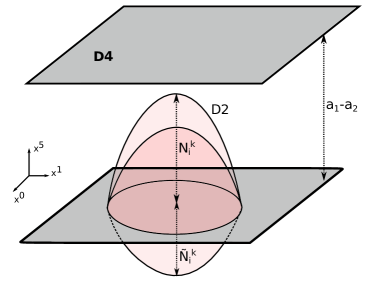
Figure 4: Geometry of composite D0 – fuzzy D2-$\overline{\text{D2}}$ bubble. Distance $N_{i}^{k}=\varepsilon\left(n_{i}^{k}+1/2\right)$. For each D4 brane at $x^{5}=a_{i}$, there could be an arbitrary number of bubbles extending to $a_{i}+\varepsilon\left(n^{k}_{i}+1/2\right)$ on one side and $a_{i}-\varepsilon\left(\tilde{n}^{j}_{i}+1/2\right)$ on the other. The only requirement is that D2 should not coincide: $n^{k}_{i}\textless n^{k+1}_{i}$

Now lets return to the monopole production. Note that the D0-D2 composites, like the original D0 brane instantons, are stretched along the $x^{4}$ direction. The only difference between them and monopoles is that monopole D2 branes are stretched all the way from one D4 to another. We conjecture that if the distance between two of the D4 branes becomes an integer multiple of $\varepsilon$, then D0-D2 may form a cylindrical D2. But cylindrical D2 brane is exactly the Euclidean configuration responsible for monopole production[94]! The formation may occur in two situations: either two D2 branes coming from different D4 touch and form a cylinder or one D2 becomes big enough to overlap the adjacent D4. In this case we have a cylinder plus an instanton starting from the adjacent D4. It is easy to see that such collisions indeed lead to poles in the Nekrasov partition function: contribution to the partition function from two D2 branes is proportional to($k,l$ simply numbers D2 branes)[93]:

$$e^{-V}=\frac{1}{a_{i}+\varepsilon n_{i}^{l}-a_{j}+\varepsilon\tilde{n}_{j}^{k}+\varepsilon}$$ (107)

Therefore if two D2 touch, it indeed leads to a pole. Apart from the potential energy (106) each D2 brane has a kinetic energy:

$$e^{K_{i}}=\prod_{l=1}^{N}\frac{1}{\left(a_{l}-a_{i}-\varepsilon\tilde{n}_{i}^{l}\right)\left(a_{l}-a_{i}-\varepsilon\left(\tilde{n}_{i}^{l}-1\right)\right)\dots\left(a_{l}-a_{i}+\varepsilon n_{i}^{l}\right)}$$ (108)

Therefore if D2 brane intersects adjacent D4, it leads to a pole too.

To further check this picture lets study a single D2 brane cap stretched between two D4 in $SU(2)$ theory. The corresponding pair of Young diagrams is just a row with $n$ boxes if $2a=\varepsilon n$ and an empty diagram. We are expecting that such configuration becomes a single cylinder stretched between two D4 and its contribution should be of order $e^{-2\pi|a_{D}^{M}|/\varepsilon}$ for large $n$. Indeed, it is easy to check that for such pair of Young diagram the Nekrasov formulas produce

$$\frac{1}{n!^{2}(n+1)!^{2}}\sim\exp\left(-\frac{4\pi|a^{M}_{D}|}{\varepsilon}\right)$$ (109)

where we have used eq. (29). Note the appearance of the same factor $\frac{1}{n!^{2}(n+1)!^{2}}$ as in eq. (33). We expect that after the resummation of an infinite number of such cylinders we will again obtain the square root function as in (33), such that the contribution of a single cylinder in indeed $e^{-2\pi|a^{M}_{D}|/\varepsilon}$.

6 Conclusions

In this paper we have analyzed the interplay between the non-perturbative tunneling effects in the QM and the fate of the naive singularities in the effective twisted superpotential of the effective two-dimensional theory. We have focused on the simplest phenomena in this context - exponentially small gaps in the QM spectrum well above the barrier. It was shown explicitly that each pole singularity gets split into the cut upon the summation over the proper terms in the instanton trans-series. This procedure corresponds to the trans-asymptotic matching procedure known in mathematical literature. In the case of pure $U(2)$ gauge theory the theory that appears in the local description was identified with the sigma model on $\mathbf{CP}^{1}$ and two SUSY vacua in 2d theory support the existence of the solitonic 2d states. Much similar to the decay of the $W$-boson in the SW theory, the $W$-boson with angular momentum $n$ decays into the pair of solitons inside the curve of marginal stability around $n$-th cut. Some partial results have been also obtained for $U(N)$ case where the corresponding local model was identified with the flag sigma-model.

The non-perturbative twisted superpotential for $SU(2)$ with fundamental or adjoint matter theory is known due to AGT correspondence to coincide with the classical conformal block. The naive pole in the superpotential corresponds to the naive pole in the classical conformal block where the intermediate dimension corresponds to the degenerate operator. We argue that near each pole the conformal block enjoys the $\mathbf{CP}^{1}$ geometry. Moreover there is a wall crossing phenomena near each pole which can thought of as the region in the space of intermediate dimensions or in the complex time plane near the operator insertion point. Using the holographic correspondence we can map near the pole geometry of the classical conformal block into the scattering of two heavy objects in $AdS_{3}$ geometry. We have argued that the poles in the scattering amplitudes corresponding to the pure winding modes in the intermediate states disappear and the cuts get developed. We predict some wall-crossing phenomena for the scattering process of conical defects and extremal black holes. However this issue deserves much more detailed study. The analogy with the non-perturbative effects in the low-energy monopole scattering involving the geodesic motion on the monopoles moduli space has been mentioned.

It is a bit surprising in spite of the resurgence arguments that the exponentially small gap in the spectrum due to the above barrier reflection which certainly is the effect of instanton–anti-instanton pairs in QM is expressed in terms of the instantons in 4d without the use of anti-instantons. To get more intuition on this subtle point we have taken a look at the Schwinger-like interpretation of the exponentially gap formation in 4d theory as some instanton–anti-instanton phenomena as well. There are arguments that the gap formation is related to Schwinger non-perturbative monopole pair creation by the graviphoton. However this point certainly deserves further analysis. Note that there is some analogy with the 4d SYM case when the effects of monopoles in 4d can be recovered upon the summation over the instantons in (4+1)d theory with one small compact dimension [95]. In our case we have recovered the effects of 2d solitons summing up the monopole loops which correspond to the bounces for the pair creation and lives effectively in 2+1 dimensions.

There are many questions to be answered. The difficult question concerns the interpolation between large and small Planck constant in QM. The regions in the moduli space around each cut enclosed by the CMS at large $\hbar$ have to be glued into the single CMS around the origin of the moduli space in SW solution at $\hbar=0$. This implies the complicated rearrangement of the wall-crossing network when $\hbar$ is decreasing. The complexification of the Planck constant discussed in [96] as well as approach suggested in [97] seem to be important for this question. The analysis of the band and gap structure in the full $\Omega$-background certainly of great interest. It corresponds to the quantization of the Whitham dynamics and being translated via AGT to Liouville theory and $AdS_{3}$ gravity concerns the non-perturbative effects in quantum 3d gravity which would generalize our consideration of the semi-classical scattering.

The generalization of the analysis for the 5d SYM gauge theory and therefore for the relativistic Toda system seems to be straightforward and the interplay between the summation over the instantons near the naive poles and summation over the torus knot invariants [98] could yield new ways to utilize the knot invariants in context of the tunneling phenomena in the quantum mechanics with difference Schrödinger equation. The interplay between the naive poles and non-perturbative completion of the theory has been discussed in ABJM theory in [99, 100]. It would be interesting to apply our approach to that case. Another interesting question concerns the possible meaning of our analysis in the hydrodynamical picture for the instanton moduli space at large $N$ [101].

The list of stable BPS objects in $\Omega$-background involves the BPS domain walls and BPS strings [102, 103, 104] which saturate the corresponding central charges in SUSY algebra. It is not clear which role these 4d states play in the sigma models near the cuts on the QM side and in the $AdS_{3}$ gravity. In particular the most pressing question concerns the interpretation of the 2d kinks in the near-pole $\mathbf{CP}^{1}$ model from the 4d viewpoint. In the worldsheet theory on the surface operator or on the non-Abelian string the kinks correspond to the trapped monopoles [105]. However in our case when we have just the dimensional reduction to 2d in the $\Omega$-background such interpretation does not work literally or at least needs some modification. Another question is: what is the counterpart of BPS domain walls and strings on the QM side? The recent development in [106] seems to be relevant for this question.

One more question concerns the issue of the ”time decay of the correlators” which becomes popular in the context of the information loss paradox starting from [107]. In the Liouville context one treats the coordinate of the vertex insertion as time-like variable and investigate the transition from the early time to late time behavior of the conformal block focusing at the subleading saddles which yield non-decaying late-time contributions. In our study we have found that there are wall-crossing phenomena near the naive poles. Hence the transition from early time to late time behavior could undergo the wall-crossing at intermediate times which is purely non-perturbative phenomena.

Appendices

Appendix A g-functions for pure $U(2)$

Here we list a few $g^{(n)}_{k}$ functions which have appeared in the main text for pure $U(2)$ theory.

• $n=1$

  $$g^{(1)}_{1}(z)=-\frac{\sqrt{4z^{2}+1}-\log\left(\frac{1}{2}\left(\sqrt{4z^{2}+1}+1\right)\right)-1}{z}$$ (110)

  $$g^{(1)}_{2}(z)=-\frac{\left(2-z^{2}\right)\sqrt{4z^{2}+1}-\left(3z^{2}+2\right)}{12z^{3}}$$ (111)

  $$g^{(1)}_{3}(z)=-\frac{\frac{127z^{4}}{288}-\frac{z^{2}}{16}+\frac{\frac{11z^{6}}{180}-\frac{599z^{4}}{1440}+\frac{13z^{2}}{80}+\frac{1}{20}}{\sqrt{4z^{2}+1}}-\frac{1}{20}}{z^{5}}$$ (112)

  $$g^{(1)}_{4}(z)=-\frac{-\frac{16985z^{6}}{20736}+\frac{1847z^{4}}{5184}-\frac{z^{2}}{64}+\frac{\frac{55z^{10}}{1008}+\frac{235z^{8}}{567}-\frac{191617z^{6}}{145152}-\frac{4343z^{4}}{36288}+\frac{71z^{2}}{448}+\frac{1}{42}}{\left(4z^{2}+1\right)^{3/2}}-\frac{1}{42}}{z^{7}}$$ (113)

• $n=2$

  $$g^{(2)}_{1}(z)=-\frac{\sqrt{z^{2}+1}-\log\left(\frac{1}{2}\left(\sqrt{z^{2}+1}+1\right)\right)-1}{z}$$ (114)

  $$g^{(2)}_{2}(z)=-\frac{8-8\sqrt{z^{2}+1}}{9z}$$ (115)

  $$g^{(2)}_{3}(z)=-\frac{-\frac{3355z^{2}}{1728}-\frac{-\frac{11141z^{4}}{5184}-\frac{3679z^{2}}{1728}-\frac{3}{8}}{\sqrt{z^{2}+1}}-\frac{3}{8}}{z^{3}}$$ (116)

• $n=3$

  $$g^{(3)}_{1}(z)=-\frac{\sqrt{\frac{z^{2}}{36}+1}-\log\left(\frac{1}{2}\left(\sqrt{\frac{z^{2}}{36}+1}+1\right)\right)-1}{z}$$ (117)

  $$g^{(3)}_{2}(z)=-\frac{3z^{2}-3z^{2}\sqrt{\frac{z^{2}}{36}+1}}{16z^{3}}$$ (118)

Appendix B Comment on two Riemann surfaces

The Lame equation at fixed coupling is a simple example of the finite-gap potential familiar in the theory of the KdV equation. In general the potential $n(n+1)\wp(x)$ corresponds to genus $n$ Riemann surface and therefore the Mathieu cosine potential which can be derived from the Weierstrass function via the Inozemtsev limit $n\rightarrow\infty$ corresponds to the infinite genus Riemann surface.

It is worth to make a comment on the place of these Riemann surfaces in our study. First of all recall that there are two Riemann surfaces in the play. The first one $P(x,y)=0$ appears at the classical level and corresponds to the fixed level of all integrals of motion $I_{k}$ in the holomorphic Hamiltonian system $I_{k}(p_{i},q_{i})=I_{k}$. For $SU(2)$ case this is genus one Riemann surface bundled over the complex energy plane. For $SU(N)$ it is higher genus Riemann surface, for instance $g=N-1$ for pure $SU(N)$ gauge theory. Upon quantization this Riemann surface becomes the operator yielding the Baxter equation acting on the ”‘wave function”’ of the single separated variable $x$:

$$P\left(x,\frac{d}{dx}\right)Q(x,I_{k})=0$$ (119)

The commutation relation between $x$ and $y$ can be more complicated and the Baxter equation can be a difference or even an integral equation. The $x$-dependence of wave function of the quantum integrable system $\Psi(x,E)$ at fixed energy or fixed integrals of motion in the many-body case is controlled by the solutions to the Baxter equation.

However there is the second Riemann surface which governs the $E$-dependence of the wave function and its genus is not related with the genus of the classical spectral curve. The potential in Schrödinger equation is treated as the initial condition for the KdV evolution and the whole KdV dynamics occurs on this finite genus Riemann surface. Let us remind how it can be obtained. Consider the Schrödinger equation with the periodic potential

$$(-\frac{d^{2}}{dx^{2}}+V(x)-E)f(x)=0$$ (120)

Two solutions of the Schrödinger equation defines the monodromy matrix $M$

$$\left(f_{1}(x+T,E),f_{2}(x+T,E)\right)=\left(f_{1}(x,E),f_{2}(x,E)\right)M$$ (121)

The Riemann surface can be written in terms of the monodromy matrix in the form

$$t^{2}-\operatorname{Tr}Mt+1=0$$ (122)

and relates the complex Bloch phase of the solution and its energy.

For the potential $V=-2\wp(x)$ the genus one Riemann surface reads as

$$y^{2}=\prod_{k=1}^{3}(E-E_{k})$$ (123)

where

$$E_{1}=\wp(\omega_{1}),\qquad E_{2}=\wp(\omega_{2}),\qquad E_{3}=\wp(\omega_{3}),$$ (124)

and $(2\omega_{1},2\omega_{3})$ are fundamental periods of $\wp$ function,$\sum\omega_{i}=0$. For the adjoint mass in the $\mathcal{N}=2^{*}$ theory $m_{ad}=\hbar n$ we have $2n$ naive poles in the superpotential which yield the $n$ cuts upon the split. For pure $\mathcal{N}=2$ SYM we have the infinite number of poles and this fits with the fact the Riemann surface for the Mathieu potential has infinite genus.

References

- [1] N. Seiberg and Edward Witten “Electric - magnetic duality, monopole condensation, and confinement in N=2 supersymmetric Yang-Mills theory” [Erratum: Nucl. Phys.B430,485(1994)] In Nucl. Phys. B426, 1994, pp. 19–52 DOI: 10.1016/0550-3213(94)90124-4, 10.1016/0550-3213(94)00449-8
- [2] Nikita A. Nekrasov “Seiberg-Witten prepotential from instanton counting” In Adv. Theor. Math. Phys. 7.5, 2003, pp. 831–864 DOI: 10.4310/ATMP.2003.v7.n5.a4
- [3] Nikita Nekrasov and Andrei Okounkov “Seiberg-Witten theory and random partitions”, 2003 arXiv:hep-th/0306238 [hep-th]
- [4] A. Gorsky et al. “Integrability and Seiberg-Witten exact solution” In Phys. Lett. B355, 1995, pp. 466–474 DOI: 10.1016/0370-2693(95)00723-X
- [5] Emil J. Martinec and Nicholas P. Warner “Integrable systems and supersymmetric gauge theory” In Nucl. Phys. B459, 1996, pp. 97–112 DOI: 10.1016/0550-3213(95)00588-9
- [6] Ron Donagi and Edward Witten “Supersymmetric Yang-Mills theory and integrable systems” In Nucl. Phys. B460, 1996, pp. 299–334 DOI: 10.1016/0550-3213(95)00609-5
- [7] A. Gorsky, A. Marshakov, A. Mironov and A. Morozov “N=2 supersymmetric QCD and integrable spin chains: Rational case N(f) ¡ 2N(c)” In Phys. Lett. B380, 1996, pp. 75–80 DOI: 10.1016/0370-2693(96)00480-7
- [8] A. Gorsky, S. Gukov and A. Mironov “Multiscale N=2 SUSY field theories, integrable systems and their stringy / brane origin. 1.” In Nucl. Phys. B517, 1998, pp. 409–461 DOI: 10.1016/S0550-3213(98)00055-8
- [9] A. Gorsky, S. Gukov and A. Mironov “SUSY field theories, integrable systems and their stringy / brane origin. 2.” In Nucl. Phys. B518, 1998, pp. 689–713 DOI: 10.1016/S0550-3213(98)00106-0
- [10] A. Gorsky, A. Marshakov, A. Mironov and A. Morozov “RG equations from Whitham hierarchy” In Nucl. Phys. B527, 1998, pp. 690–716 DOI: 10.1016/S0550-3213(98)00315-0
- [11] Nikita A. Nekrasov and Samson L. Shatashvili “Quantum integrability and supersymmetric vacua” In 30 years of mathematical methods in high energy physics. Proceedings, International Conference in honor of Professor Tohru Eguchi’s 60th birthday, Kyoto, Japan, March 17-19, 2008 177, 2009, pp. 105–119 DOI: 10.1143/PTPS.177.105
- [12] Nikita A. Nekrasov and Samson L. Shatashvili “Supersymmetric vacua and Bethe ansatz” In Cargese 2008, theory and particle physics : The LHC perspective and beyond, proceedings of the ESF School in High Energy Physics and Astrophysics, Cargese Summer School, Cargese, France, 16-28 June 2008 192-193, 2009, pp. 91–112 DOI: 10.1016/j.nuclphysbps.2009.07.047
- [13] Nikita A. Nekrasov and Samson L. Shatashvili “Quantization of Integrable Systems and Four Dimensional Gauge Theories” In Proceedings, 16th International Congress on Mathematical Physics (ICMP09): Prague, Czech Republic, August 3-8, 2009, 2009, pp. 265–289 DOI: 10.1142/9789814304634˙0015
- [14] Nikita Nekrasov and Edward Witten “The Omega Deformation, Branes, Integrability, and Liouville Theory” In JHEP 09, 2010, pp. 092 DOI: 10.1007/JHEP09(2010)092
- [15] Ovidiu Costin “Asymptotics and Borel summability” CRC press, 2008
- [16] Gokce Basar and Gerald V. Dunne “Hydrodynamics, resurgence, and transasymptotics” In Phys. Rev. D92.12, 2015, pp. 125011 DOI: 10.1103/PhysRevD.92.125011
- [17] N. Dorey “The BPS spectra of two-dimensional supersymmetric gauge theories with twisted mass terms” In JHEP 11, 1998, pp. 005 DOI: 10.1088/1126-6708/1998/11/005
- [18] M. Shifman, A. Vainshtein and Roman Zwicky “Central charge anomalies in 2-D sigma models with twisted mass” In J. Phys. A39, 2006, pp. 13005–13024 DOI: 10.1088/0305-4470/39/41/S13
- [19] Luis F. Alday, Davide Gaiotto and Yuji Tachikawa “Liouville Correlation Functions from Four-dimensional Gauge Theories” In Lett.Math.Phys. 91, 2010, pp. 167–197 DOI: 10.1007/s11005-010-0369-5
- [20] Marcin Piatek and Artur R. Pietrykowski “Classical limit of irregular blocks and Mathieu functions” In JHEP 01, 2016, pp. 115 DOI: 10.1007/JHEP01(2016)115
- [21] Marcin Piatek “Classical torus conformal block, twisted superpotential and the accessory parameter of Lamé equation” In JHEP 03, 2014, pp. 124 DOI: 10.1007/JHEP03(2014)124
- [22] Vladimir A. Fateev, A. V. Litvinov, Andre Neveu and Enrico Onofri “Differential equation for four-point correlation function in Liouville field theory and elliptic four-point conformal blocks” In J. Phys. A42, 2009, pp. 304011 DOI: 10.1088/1751-8113/42/30/304011
- [23] Rubik Poghossian “Deforming SW curve” In JHEP 04, 2011, pp. 033 DOI: 10.1007/JHEP04(2011)033
- [24] V. A. Fateev and A. V. Litvinov “On AGT conjecture” In JHEP 02, 2010, pp. 014 DOI: 10.1007/JHEP02(2010)014
- [25] Davide Gaiotto “Asymptotically free theories and irregular conformal blocks” In Proceedings, 6th International Symposium on Quantum Theory and Symmetries (QTS6): Lexington, Kentucky, USA, July 20-25, 2009 462.1, 2013, pp. 012014 DOI: 10.1088/1742-6596/462/1/012014
- [26] Per Kraus “Lectures on black holes and the AdS(3) / CFT(2) correspondence” In Lect. Notes Phys. 755, 2008, pp. 193–247 arXiv:hep-th/0609074 [hep-th]
- [27] A. Liam Fitzpatrick, Jared Kaplan and Matthew T. Walters “Universality of Long-Distance AdS Physics from the CFT Bootstrap” In JHEP 08, 2014, pp. 145 DOI: 10.1007/JHEP08(2014)145
- [28] Curtis T. Asplund, Alice Bernamonti, Federico Galli and Thomas Hartman “Holographic Entanglement Entropy from 2d CFT: Heavy States and Local Quenches” In JHEP 02, 2015, pp. 171 DOI: 10.1007/JHEP02(2015)171
- [29] Eliot Hijano, Per Kraus and River Snively “Worldline approach to semi-classical conformal blocks” In JHEP 07, 2015, pp. 131 DOI: 10.1007/JHEP07(2015)131
- [30] A. Liam Fitzpatrick and Jared Kaplan “On the Late-Time Behavior of Virasoro Blocks and a Classification of Semiclassical Saddles” In JHEP 04, 2017, pp. 072 DOI: 10.1007/JHEP04(2017)072
- [31] A. Liam Fitzpatrick, Jared Kaplan, Matthew T. Walters and Junpu Wang “Hawking from Catalan” In JHEP 05, 2016, pp. 069 DOI: 10.1007/JHEP05(2016)069
- [32] K. B. Alkalaev and V. A. Belavin “Holographic duals of large-c torus conformal blocks” In JHEP 10, 2017, pp. 140 DOI: 10.1007/JHEP10(2017)140
- [33] K. B. Alkalaev and V. A. Belavin “Holographic interpretation of 1-point toroidal block in the semiclassical limit” In JHEP 06, 2016, pp. 183 DOI: 10.1007/JHEP06(2016)183
- [34] Kirill Krasnov “Lambda less than 0 quantum gravity in (2+1)-dimensions. 2. Black hole creation by point particles” In Class. Quant. Grav. 19, 2002, pp. 3999–4028 DOI: 10.1088/0264-9381/19/15/309
- [35] Kirill Krasnov “Lambda less than 0 quantum gravity in 2+1 dimensions. 1. Quantum states and stringy S matrix” In Class. Quant. Grav. 19, 2002, pp. 3977–3998 DOI: 10.1088/0264-9381/19/15/308
- [36] M. F. Atiyah and Nigel J. Hitchin “Low-Energy Scattering of Nonabelian Monopoles” In Phys. Lett. A107, 1985, pp. 21–25 DOI: 10.1016/0375-9601(85)90238-5
- [37] A. Achucarro and P. K. Townsend “A Chern-Simons Action for Three-Dimensional anti-De Sitter Supergravity Theories” In Phys. Lett. B180, 1986, pp. 89 DOI: 10.1016/0370-2693(86)90140-1
- [38] Edward Witten “(2+1)-Dimensional Gravity as an Exactly Soluble System” In Nucl. Phys. B311, 1988, pp. 46 DOI: 10.1016/0550-3213(88)90143-5
- [39] Gökçe Başar and Gerald V. Dunne “Resurgence and the Nekrasov-Shatashvili limit: connecting weak and strong coupling in the Mathieu and Lamé systems” In JHEP 02, 2015, pp. 160 DOI: 10.1007/JHEP02(2015)160
- [40] Matteo Beccaria “On the large -deformations in the Nekrasov-Shatashvili limit of SYM” In JHEP 07, 2016, pp. 055 DOI: 10.1007/JHEP07(2016)055
- [41] Saebyeok Jeong “Splitting of surface defect partition functions and integrable systems”, 2017 arXiv:1709.04926 [hep-th]
- [42] Sergei L. Lukyanov “Critical values of the Yang-Yang functional in the quantum sine-Gordon model” In Nucl. Phys. B853, 2011, pp. 475–507 DOI: 10.1016/j.nuclphysb.2011.07.028
- [43] Gregory W. Moore, Nikita Nekrasov and Samson Shatashvili “Integrating over Higgs branches” In Commun. Math. Phys. 209, 2000, pp. 97–121 DOI: 10.1007/PL00005525
- [44] Anton A. Gerasimov and Samson L. Shatashvili “Two-dimensional gauge theories and quantum integrable systems” In Proceedings of Symposia in Pure Mathematics, May 25-29 2007, University of Augsburg, Germany, 2007 arXiv: http://inspirehep.net/record/767222/files/arXiv:0711.1472.pdf
- [45] Anton A. Gerasimov and Samson L. Shatashvili “Higgs Bundles, Gauge Theories and Quantum Groups” In Commun. Math. Phys. 277, 2008, pp. 323–367 DOI: 10.1007/s00220-007-0369-1
- [46] Nikita Nekrasov “BPS/CFT correspondence: non-perturbative Dyson-Schwinger equations and qq-characters” In JHEP 03, 2016, pp. 181 DOI: 10.1007/JHEP03(2016)181
- [47] Nikita Nekrasov and Vasily Pestun “Seiberg-Witten geometry of four dimensional N=2 quiver gauge theories”, 2012 arXiv:1211.2240 [hep-th]
- [48] Nikita Nekrasov, Vasily Pestun and Samson Shatashvili “Quantum geometry and quiver gauge theories”, 2013 arXiv:1312.6689 [hep-th]
- [49] Marco Matone “Instantons and recursion relations in N=2 SUSY gauge theory” In Phys. Lett. B357, 1995, pp. 342–348 DOI: 10.1016/0370-2693(95)00920-G
- [50] Rainald Flume, Francesco Fucito, Jose F. Morales and Rubik Poghossian “Matone’s relation in the presence of gravitational couplings” In JHEP 04, 2004, pp. 008 DOI: 10.1088/1126-6708/2004/04/008
- [51] A. Gorsky and A. Milekhin “RG-Whitham dynamics and complex Hamiltonian systems” In Nucl. Phys. B895, 2015, pp. 33–63 DOI: 10.1016/j.nuclphysb.2015.03.028
- [52] Davide Gaiotto, Sergei Gukov and Nathan Seiberg “Surface Defects and Resolvents” In JHEP 1309, 2013, pp. 070 DOI: 10.1007/JHEP09(2013)070
- [53] Davide Gaiotto “Surface Operators in N = 2 4d Gauge Theories” In JHEP 1211, 2012, pp. 090 DOI: 10.1007/JHEP11(2012)090
- [54] A. Gorsky, B. Le Floch, A. Milekhin and N. Sopenko “Surface defects and instanton–vortex interaction” In Nucl. Phys. B920, 2017, pp. 122–156 DOI: 10.1016/j.nuclphysb.2017.04.010
- [55] S. K. Ashok et al. “Surface operators, chiral rings and localization in =2 gauge theories” In JHEP 11, 2017, pp. 137 DOI: 10.1007/JHEP11(2017)137
- [56] S. K. Ashok et al. “Modular and duality properties of surface operators in N=2* gauge theories” In JHEP 07, 2017, pp. 068 DOI: 10.1007/JHEP07(2017)068
- [57] Sergio Cecotti and Cumrun Vafa “On classification of N=2 supersymmetric theories” In Commun. Math. Phys. 158, 1993, pp. 569–644 DOI: 10.1007/BF02096804
- [58] Davide Gaiotto, Gregory W. Moore and Andrew Neitzke “Wall-Crossing in Coupled 2d-4d Systems” In JHEP 12, 2012, pp. 082 DOI: 10.1007/JHEP12(2012)082
- [59] Kentaro Hori and Cumrun Vafa “Mirror symmetry”, 2000 arXiv:hep-th/0002222 [hep-th]
- [60] Sergey Shadchin “On F-term contribution to effective action” In JHEP 08, 2007, pp. 052 DOI: 10.1088/1126-6708/2007/08/052
- [61] Nikita A. Nekrasov “Instanton partition functions and M-theory” In Proceedings, 15th International Seminar on High Energy Physics (Quarks 2008): Sergiev Posad, Russia. May 23-29, 2008, 2008 URL: http://quarks.inr.ac.ru/2008/proceedings/p5_FT/nekrasov.pdf
- [62] Tudor Dimofte, Sergei Gukov and Lotte Hollands “Vortex Counting and Lagrangian 3-manifolds” In Lett. Math. Phys. 98, 2011, pp. 225–287 DOI: 10.1007/s11005-011-0531-8
- [63] Nima Doroud, Jaume Gomis, Bruno Le Floch and Sungjay Lee “Exact Results in D=2 Supersymmetric Gauge Theories” In JHEP 05, 2013, pp. 093 DOI: 10.1007/JHEP05(2013)093
- [64] Al B Zamolodchikov “Conformal symmetry in two-dimensional space: recursion representation of conformal block” In Theoretical and Mathematical Physics 73.1 Springer, 1987, pp. 1088–1093
- [65] João Penedones, Emilio Trevisani and Masahito Yamazaki “Recursion Relations for Conformal Blocks” In JHEP 09, 2016, pp. 070 DOI: 10.1007/JHEP09(2016)070
- [66] Ferdinando Gliozzi, Andrea L. Guerrieri, Anastasios C. Petkou and Congkao Wen “The analytic structure of conformal blocks and the generalized Wilson-Fisher fixed points” In JHEP 04, 2017, pp. 056 DOI: 10.1007/JHEP04(2017)056
- [67] J. Teschner “Quantization of the Hitchin moduli spaces, Liouville theory, and the geometric Langlands correspondence I” In Adv. Theor. Math. Phys. 15.2, 2011, pp. 471–564 DOI: 10.4310/ATMP.2011.v15.n2.a6
- [68] J. Teschner “Quantization of moduli spaces of flat connections and Liouville theory” In International Congress of Mathematicians (ICM 2014) Seoul, Korea, August 13-21, 2014, 2014 arXiv: http://inspirehep.net/record/1293937/files/arXiv:1405.0359.pdf
- [69] J. Zinn-Justin and U. D. Jentschura “Multi-instantons and exact results I: Conjectures, WKB expansions, and instanton interactions” In Annals Phys. 313, 2004, pp. 197–267 DOI: 10.1016/j.aop.2004.04.004
- [70] Gerald V. Dunne and Mithat Unsal “Resurgence and Trans-series in Quantum Field Theory: The CP(N-1) Model” In JHEP 11, 2012, pp. 170 DOI: 10.1007/JHEP11(2012)170
- [71] Gokce Basar, Gerald V. Dunne and Mithat Unsal “Quantum Geometry of Resurgent Perturbative/Nonperturbative Relations” In JHEP 05, 2017, pp. 087 DOI: 10.1007/JHEP05(2017)087
- [72] Santiago Codesido and Marcos Marino “Holomorphic Anomaly and Quantum Mechanics”, 2016 arXiv:1612.07687 [hep-th]
- [73] Edward Witten “Coadjoint Orbits of the Virasoro Group” In Commun. Math. Phys. 114, 1988, pp. 1 DOI: 10.1007/BF01218287
- [74] J. Balog, L. Feher and L. Palla “Coadjoint orbits of the Virasoro algebra and the global Liouville equation” In Int. J. Mod. Phys. A13, 1998, pp. 315–362 DOI: 10.1142/S0217751X98000147
- [75] A. Alekseev and Samson L. Shatashvili “Path Integral Quantization of the Coadjoint Orbits of the Virasoro Group and 2D Gravity” In Nucl. Phys. B323, 1989, pp. 719–733 DOI: 10.1016/0550-3213(89)90130-2
- [76] J. David Brown and M. Henneaux “Central Charges in the Canonical Realization of Asymptotic Symmetries: An Example from Three-Dimensional Gravity” In Commun. Math. Phys. 104, 1986, pp. 207–226 DOI: 10.1007/BF01211590
- [77] Eliot Hijano, Per Kraus, Eric Perlmutter and River Snively “Semiclassical Virasoro blocks from AdS3 gravity” In JHEP 12, 2015, pp. 077 DOI: 10.1007/JHEP12(2015)077
- [78] Eliot Hijano, Per Kraus, Eric Perlmutter and River Snively “Witten Diagrams Revisited: The AdS Geometry of Conformal Blocks” In JHEP 01, 2016, pp. 146 DOI: 10.1007/JHEP01(2016)146
- [79] Juan Martin Maldacena “Eternal black holes in anti-de Sitter” In JHEP 04, 2003, pp. 021 DOI: 10.1088/1126-6708/2003/04/021
- [80] Steven Carlip “Quantum gravity in 2+1 dimensions: The Case of a closed universe” In Living Rev. Rel. 8, 2005, pp. 1 DOI: 10.12942/lrr-2005-1
- [81] Atanu Bhatta, Prashanth Raman and Nemani V. Suryanarayana “Holographic Conformal Partial Waves as Gravitational Open Wilson Networks” In JHEP 06, 2016, pp. 119 DOI: 10.1007/JHEP06(2016)119
- [82] Mert Besken, Ashwin Hegde, Eliot Hijano and Per Kraus “Holographic conformal blocks from interacting Wilson lines” In JHEP 08, 2016, pp. 099 DOI: 10.1007/JHEP08(2016)099
- [83] Herman L. Verlinde “Conformal Field Theory, 2- Quantum Gravity and Quantization of Teichmuller Space” In Nucl. Phys. B337, 1990, pp. 652–680 DOI: 10.1016/0550-3213(90)90510-K
- [84] Andrei Mikhailov, Nikita Nekrasov and Savdeep Sethi “Geometric realizations of BPS states in N=2 theories” In Nucl. Phys. B531, 1998, pp. 345–362 DOI: 10.1016/S0550-3213(98)80001-1
- [85] Hongbin Chen et al. “Degenerate Operators and the Expansion: Lorentzian Resummations, High Order Computations, and Super-Virasoro Blocks” In JHEP 03, 2017, pp. 167 DOI: 10.1007/JHEP03(2017)167
- [86] A. Liam Fitzpatrick and Jared Kaplan “A Quantum Correction To Chaos” In JHEP 05, 2016, pp. 070 DOI: 10.1007/JHEP05(2016)070
- [87] JNL Connor, T Uzer, RA Marcus and AD Smith “Eigenvalues of the Schrödinger equation for a periodic potential with nonperiodic boundary conditions: A uniform semiclassical analysis” In The Journal of chemical physics 80.10 AIP, 1984, pp. 5095–5106
- [88] Rajesh Gopakumar and Cumrun Vafa “M theory and topological strings. 1.”, 1998 arXiv:hep-th/9809187 [hep-th]
- [89] Rajesh Gopakumar and Cumrun Vafa “M theory and topological strings. 2.”, 1998 arXiv:hep-th/9812127 [hep-th]
- [90] Mykola Dedushenko and Edward Witten “Some Details On The Gopakumar-Vafa and Ooguri-Vafa Formulas” In Adv. Theor. Math. Phys. 20, 2016, pp. 1–133 DOI: 10.4310/ATMP.2016.v20.n1.a1
- [91] A. Mironov and A. Morozov “Nekrasov Functions and Exact Bohr-Zommerfeld Integrals” In JHEP 04, 2010, pp. 040 DOI: 10.1007/JHEP04(2010)040
- [92] Amir-Kian Kashani-Poor and Jan Troost “Pure super Yang-Mills and exact WKB” In JHEP 08, 2015, pp. 160 DOI: 10.1007/JHEP08(2015)160
- [93] So Matsuura “Instanton Counting and Dielectric Branes” In Proceedings, 20th International Conference on Ultra-Relativistic Nucleus-Nucleus Collisions (QM 2008): Jaipur, India, February 4-10, 2008 09, 2008, pp. 083 DOI: 10.1088/1126-6708/2008/09/083
- [94] A. S. Gorsky, K. A. Saraikin and K. G. Selivanov “Schwinger type processes via branes and their gravity duals” In Nucl. Phys. B628, 2002, pp. 270–294 DOI: 10.1016/S0550-3213(02)00095-0
- [95] Albion E. Lawrence and Nikita Nekrasov “Instanton sums and five-dimensional gauge theories” In Nucl.Phys. B513, 1998, pp. 239–265 DOI: 10.1016/S0550-3213(97)00694-9
- [96] Alba Grassi and Marcos Marino “The complex side of the TS/ST correspondence”, 2017 arXiv:1708.08642 [hep-th]
- [97] Ricardo Couso-Santamaría, Marcos Marino and Ricardo Schiappa “Resurgence Matches Quantization” In J. Phys. A50.14, 2017, pp. 145402 DOI: 10.1088/1751-8121/aa5e01
- [98] A. Gorsky, A. Milekhin and N. Sopenko “The Condensate from Torus Knots” In JHEP 09, 2015, pp. 102 DOI: 10.1007/JHEP09(2015)102
- [99] Nadav Drukker, Marcos Marino and Pavel Putrov “Nonperturbative aspects of ABJM theory” In JHEP 11, 2011, pp. 141 DOI: 10.1007/JHEP11(2011)141
- [100] Nadav Drukker, Marcos Marino and Pavel Putrov “From weak to strong coupling in ABJM theory” In Commun. Math. Phys. 306, 2011, pp. 511–563 DOI: 10.1007/s00220-011-1253-6
- [101] Giulio Bonelli, Antonio Sciarappa, Alessandro Tanzini and Petr Vasko “Quantum Cohomology and Quantum Hydrodynamics from Supersymmetric Quiver Gauge Theories” In J. Geom. Phys. 109, 2016, pp. 3–43 DOI: 10.1016/j.geomphys.2015.10.001
- [102] Simeon Hellerman, Domenico Orlando and Susanne Reffert “String theory of the Omega deformation” In JHEP 01, 2012, pp. 148 DOI: 10.1007/JHEP01(2012)148
- [103] Simeon Hellerman, Domenico Orlando and Susanne Reffert “The Omega Deformation From String and M-Theory” In JHEP 07, 2012, pp. 061 DOI: 10.1007/JHEP07(2012)061
- [104] Kseniya Bulycheva, Heng-Yu Chen, Alexander Gorsky and Peter Koroteev “BPS States in Omega Background and Integrability” In JHEP 10, 2012, pp. 116 DOI: 10.1007/JHEP10(2012)116
- [105] David Tong “Monopoles in the higgs phase” In Phys. Rev. D69, 2004, pp. 065003 DOI: 10.1103/PhysRevD.69.065003
- [106] Mathew Bullimore, Hee-Cheol Kim and Tomasz Lukowski “Expanding the Bethe/Gauge Dictionary” In JHEP 11, 2017, pp. 055 DOI: 10.1007/JHEP11(2017)055
- [107] Stephen H. Shenker and Douglas Stanford “Black holes and the butterfly effect” In JHEP 03, 2014, pp. 067 DOI: 10.1007/JHEP03(2014)067