Layered Non-Orthogonal Random Access with SIC and Transmit Diversity for Reliable Transmissions

Abstract

In this paper, we study a layered random access scheme based on non-orthogonal multiple access (NOMA) to improve the throughput of multichannel ALOHA. At a receiver, successive interference cancellation (SIC) is carried out across layers to remove the signals that are already decoded. A closed-form expression for the total throughput is derived under certain assumptions. It is shown that the transmission rates of layers can be optimized to maximize the total throughput and the proposed scheme can improve the throughput with multiple layers. Furthermore, it is shown that the optimal rates can be recursively found using multiple individual one-dimensional optimizations. We also modify the proposed layered random access scheme with contention resolution repetition diversity for reliable transmissions with a delay constraint. It is shown to be possible to have a low outage probability if the number of copies can be optimized, which is desirable for high reliability low latency communications.

I Introduction

In order to support massive connectivity in machine-type communications (MTC), random access has been considered in cellular standards [1] [2]. In particular, ALOHA [3] [4] is mainly studied for random access in MTC with multiple channels, which is multichannel ALOHA [5]. In [6] [7], the performance of multichannel ALOHA has also been analyzed and optimized for MTC. In [8], it is shown that the number of channels can be adaptively decided to maximize the throughput if the number of channels is flexible.

Successive interference cancellation (SIC) can be employed to improve the throughput when a tree algorithm is used for random access as in [9]. In [10], within a frame, a packet is repeatedly transmitted to exploit contention resolution repetition diversity (CRRD) together with SIC. If there is one copy of a packet that can be transmitted without collision, it can be successfully decoded and its copies can be removed. This process can be repeated at a receiver, which can result in the throughput improvement. In [11] [12][13], further improvements are made using graph-based analysis for irregular repetition of coded packets. The resulting approach is referred to as irregular repetition slotted ALOHA (IRSA).

While the approaches in [9] assume a simple channel model without taking into account fading, it might be necessary to consider fading channels in random access over wireless channels. In this case, SIC can be considered in the context of non-orthogonal multiple access (NOMA) where the power difference is to be exploited [14] [15] [16]. In [17], a NOMA based random access method is proposed where each user can randomly choose a channel as well as a power level. In this case, although two users choose the same channel, a receiver (or base station (BS) for uplink transmissions) can recover both signals using SIC if they choose different power levels. Thus, the throughput can be improved. In [18], NOMA is also used for random access based on the power control scheme proposed in [19].

In this paper, we study a NOMA based random access as in [17] to improve the throughput of multichannel ALOHA by exploiting the power difference. The resulting random access scheme can be seen as a layered random access scheme where each layer is characterized by the power level. However, unlike [17], we assume that users do not know their channel state information (CSI). We derive a closed-form expression for the throughput in terms of transmission rates under Rayleigh fading channels. This closed-form expression allows us to find the optimal rates that maximize the total throughput.

Although the proposed random access scheme in this paper relies on SIC as IRSA, there are a few key differences. The proposed scheme does not use iterative decoding, which is used in [11] [12][13]. Thus, the decoding delay at a receiver is fixed. In terms of interference cancellation, the main difference is that the proposed scheme uses inter-layer interference cancellation, which is SIC across layers. On the other hand, IRSA uses intra-layer interference cancellation (as there is only one layer), where interference cancellation is repeatedly carried out until no more signals are decodable. Furthermore, along with SIC, the proposed scheme exploits the capture effect, which is considered in [20] [21] to exploit the near/far effect, while IRSA does not consider the capture effect. In this paper, the capture effect is induced by the power difference for NOMA.

We also consider a modification of the proposed scheme with CRRD where multiple copies of a packet are transmitted through randomly selected different channels. Unlike the approaches in [11] [12][13], the main aim of this modification (with CRRD) is to guarantee a packet delivery subject to a delay constraint with a high probability, not to improve the throughput. However, as there are multiple layers, the overall throughput can be reasonably high once SIC is successfully used. The resulting approach may be useful for high reliable low latency communications [22][23].

The rest of the paper is organized as follows. In Section II, we present the system model for random access over fading channels and introduce the proposed layered random access scheme. We study the throughput of the proposed scheme in Section III, where the proposed scheme is also briefly compared with IRSA. In Section IV, the proposed scheme is modified with random CRRD for reliable transmissions with a delay constraint. Simulation results are shown in Section II and the paper is finally concluded with some remarks in Section VI.

Notation

Matrices and vectors are denoted by upper- and lower-case boldface letters, respectively. The superscript ${\rm T}$ denotes the transpose. The 2-norm is denoted by $||{\bf a}||$. ${\mathbb{E}}[\cdot]$ and ${\rm Var}(\cdot)$ denote the statistical expectation and variance, respectively. ${\cal C}{\cal N}({\bf a},{\bf R})$ represents the distribution of a circularly symmetric complex Gaussian (CSCG) random vector with mean vector ${\bf a}$ and covariance matrix ${\bf R}$.

II System Model

In this section, we present the system model for layered random access and explain a receiver algorithm that is based on SIC.

II-A Layered Random Access

Suppose that a system consists of one BS and a number of users for random access with multiple channels in a time slot, which might be equivalent to a multiple access control (MAC) frame in [11] [12][13]. To improve the throughput, we consider multiple layers for each channel by exploiting the notion of NOMA.

We assume that there are $L$ layers and each layer, which is characterized by a different power level, consists of $N$ orthogonal channels in a time slot. An active user that has a packet to transmit is to randomly choose a channel and one of $L$ layers in the selected channel. Let ${\cal I}_{l,q}$ denote the index set of the users that choose channel $q$ and layer $l$. In addition, denote by $h_{k,q}$ and $d_{k}$ the channel coefficient and data symbol from user $k$ to the BS, respectively, provided that user $k$ chooses channel $q$. Throughout the paper, we assume block-fading channels [24] where the channel coefficients, $h_{k,q}$, remain unchanged within a time slot. Then, the received signal at the BS through channel $q$ is given by

$$y_{q}=\sum_{l=1}^{L}s_{l,q}+n_{q},$$ (1)

where $n_{q}\sim{\cal C}{\cal N}(0,N_{0})$ is the background noise and $s_{l,q}=\sum_{k\in{\cal I}_{l,q}}\sqrt{P_{l}}h_{k,q}d_{k}$. Here, $P_{l}$ is the transmit power of layer $l$, which is a design parameter. Here, we assume that ${\mathbb{E}}[|d_{k}|^{2}]=1$ and ${\mathbb{E}}[d_{k}]=0$. If a user chooses layer $l$, the signal power has to be set to $P_{l}$.

Note that if $L=1$, the resulting system becomes the conventional single-channel slotted ALOHA system. Throughput the paper, we assume coded signals from users. If a user chooses layer $l$, the transmission (or code) rate is set to $R_{l}$. Together with $P_{l}$, $R_{l}$ is also a design parameter.

II-B Signal Decoding using SIC

Let

$$x_{l,q}=s_{l,q}+n_{l,q},$$ (2)

where $n_{l,q}$ is the interference (plus-noise) term in layer $l$, which is given by

$$n_{l,q}=\sum_{i=l+1}^{L}s_{i,q}+n_{q}.$$

Clearly, $x_{1,q}=y_{q}$ and $n_{L,q}=n_{q}$. If there are multiple signals in $x_{l,q}$, we may assume that the receiver cannot decode any signal due to packet collision. However, if there is only one signal and the interference is sufficiently weak in layer $l$ (provided that the signals in layers $1,\ldots l-1$ are removed), the receiver can decode the signal. Let $\beta_{l}$ denote the conditional probability of decoding error at layer $l$ when there is only one signal from user $k$ at channel $q$ under the lower-interference-free condition. Then, at channel $q$, assuming that capacity achieving codes are used, we have

$$\beta_{l}=\Pr\left(\log_{2}\left(1+\frac{P_{l}|h_{k,q}|^{2}}{\sigma_{l,q}^{2}}\right)<R_{l}\right),$$ (3)

where $\sigma_{l,q}^{2}={\rm Var}(n_{l,q}\,|\,\{h_{k,q}\})={\mathbb{E}}[|n_{l,q}|^{2}\,|\,\{h_{k,q}\}]$ is the conditional variance of $n_{l,q}$.

At each channel, from layer 1 to layer $L$, the receiver performs decoding with SIC. If there is no signal or one signal that can be decoded and subtracted, the receiver can move to the next layer in each channel. However, if there is packet collision or a signal that cannot be decoded at a certain layer, the receiver stops SIC.

In Fig. 1, we illustrate a set of the channels of layered random access with $L=2$ layers and $N=10$ channels (per layer). At channel 1, there is no signal in the first layer, but in the second layer. Thus, the signal in the second layer is decodable if the signal-to-noise ratio (SNR) is sufficiently high. At channel 2, there are two signals. However, they are in different layers. Thus, the BS is able to decode the signal in the first layer if the signal-to-interference-plus-noise ratio (SINR) is sufficiently high. Once the signal in the first layer is decoded, it can be removed using SIC and the signal in the second layer can be decoded if its SNR is sufficiently high. At channel 3, there are also two signals, but both are in the second layer, which results in packet collision. Thus, the two signals may not be decodable.

Figure 1: Multiple channels of layered random access access with $L=2$ layers and $N=10$ channels (per layer).

In [17], by exploiting the power difference, NOMA is applied to multichannel ALOHA, which becomes the layered random access scheme in this section. While it is assumed that the users know their CSI so that they can decide the transmit powers to allow SIC and guarantee successful decoding if there is no collision in [17], we do not assume CSI at transmitters (i.e., users) in this paper. Consequently, the success of SIC depends on both packet collision and (instantaneous) CSI, and the throughput analysis becomes more involved than that in [17]. In the next section, we study the performance analysis under certain assumptions.

III Throughput Analysis

We consider the following assumptions in this section for the throughput analysis.

• The number of arrivals at layer $l$ or the number of the users that choose layer $l$, denoted by $M_{l}$, is an independent Poisson random variable with mean $\lambda_{l}$, which is the (average) arrival rate at layer $l$, i.e.,

  $$\Pr(M_{l}=m) =P_{l}(m)$$

  $$=\frac{\lambda_{l}^{m}e^{-\lambda_{l}}}{m!},\ m=0,1,\ldots$$

  Note that the average number of users becomes $\sum_{l=1}^{L}\lambda_{l}$. Thus, if the average number of users is fixed, the average number of users in each layer, $\lambda_{l}$, can decrease with $L$.

• An active user is to uniformly and randomly choose a layer and a channel within the selected layer.

• If multiple users choose the same channel in the same layer, the receiver is not able to recover any signals and declares packet collision.

III-A Derivation of Throughput

Consider layer $l$ and assume that all the signals in the lower layers, i.e., from layer 1 to layer $l-1$, are successfully decoded. Then, under the assumption of A3, the conditional probability of collision or decoding error for given $m$ transmitted signals in layer $l$ is given by

$$\alpha_{l}(m)=p_{\rm c}(m)+\left(1-p_{\rm c}(m)\right)\beta_{l},$$ (4)

where $p_{\rm c}(m)$ is the (conditional) probability of packet collision at layer $l$ for given $m$ transmitted signals in layer $l$. Under A2, we have

$$p_{\rm c}(m)=1-\left(1-\frac{1}{N}\right)^{m-1},$$ (5)

which is independent of $l$.

Lemma 1

Let $\eta_{l}$ denote the average number of successfully decoded packets at layer $l$ provided that any signals in layers 1 to $l-1$ are removed by SIC. For convenience, this condition is referred to as the lower-interference-free condition for layer $l$. Then, under the assumption of A1, we have

$$\eta_{l}=\varphi_{l}\lambda_{l}e^{-\frac{\lambda_{l}}{N}},$$ (6)

where $\varphi_{l}=1-\beta_{l}=\Pr\left(\log_{2}\left(1+\frac{P_{l}|h_{k,q}|^{2}}{\sigma_{l,q}^{2}}\right)\geq R_{l}\right)$.

Proof:

See Appendix A. ∎

If $L=1$, the throughput is given by

$${\cal T}=R_{1}\eta_{1}=R_{1}\varphi_{1}\lambda_{1}e^{-\frac{\lambda_{1}}{N}}.$$ (7)

The dimension of the throughput is the same as that of $R_{1}$, which is the bits per channel use. Note that $\lambda_{1}e^{-\frac{\lambda_{1}}{N}}$ is often regarded as the throughput of multichannel ALOHA [5] (which is the average number of packets without packet collision) under the ideal collision channel model [4].

Let $\rho_{l}$ denote the probability that there is no transmitted signal or a transmitted signal is decoded through a given channel in layer $l$ under the lower-interference-free condition. Then, for a given channel, provided that there are $M_{l}=m$ signals, the conditional probability that there is no transmitted signal is $\left(1-\frac{1}{N}\right)^{m}$ and the conditional probability that there is a transmitted signal which is decodable is $(1-\beta_{l})\binom{m}{1}\frac{1}{N}\left(1-\frac{1}{N}\right)^{m-1}$. Then, $\rho_{l}$ can be found by taking the expectation over $M_{l}$, which is given by

$$\rho_{l} = {\mathbb{E}}\left[\left(1-\frac{1}{N}\right)^{M_{l}}+\varphi_{l}\binom{M_{l}}{1}\frac{1}{N}\left(1-\frac{1}{N}\right)^{M_{l}-1}\right]$$ (8)

$$= \sum_{m=0}^{\infty}\left(\left(1-\frac{1}{N}\right)^{m}+\frac{\varphi_{l}m}{N}\left(1-\frac{1}{N}\right)^{m-1}\right)$$ (10)

$$\quad\times P_{l}(m)$$

$$= \left(1+\frac{\varphi_{l}\lambda_{l}}{N}\right)e^{-\frac{\lambda_{l}}{N}}.$$ (11)

Suppose that $L=2$. Since the numbers of users in layers 1 and 2 are independent, the throughput of layer 2 becomes $R_{2}\rho_{1}\eta_{2}$. Thus, the total throughput (with $L=2$) becomes $R_{1}\eta_{1}+R_{2}\rho_{1}\eta_{2}$. Unfortunately, this total throughput is an approximation since the throughput of each layer is correlated. To see this clearly, with $L=2$, we can consider the case that users $1$ and $2$ send signals through the first channel in different layers. In this case, the probability that the BS can decode both signals becomes

$$\varphi_{1,2}=\Pr\left(\frac{P_{1}|h_{1,1}|^{2}}{P_{2}|h_{2,1}|^{2}+N_{0}}\geq\nu(R_{1}),\frac{P_{2}|h_{2,1}|^{2}}{N_{0}}\geq\nu(R_{2})\right),$$

where $\nu(R)=2^{R}-1$. Clearly, $\varphi_{1,2}\neq\varphi_{1}\varphi_{2}$. However, if we assume that the events of successful decoding in different layers are independent (provided that there is only one signal in each layer at the same channel), the throughput can be approximated by $R_{1}\eta_{1}+R_{2}\rho_{1}\eta_{2}$. In general, for $L\geq 1$, the total throughput can be approximated by ${\cal T}$ that is given by

$${\cal T} =R_{1}\eta_{1}+R_{2}\rho_{1}\eta_{2}+\ldots+R_{L}\left(\prod_{m=1}^{L-1}\rho_{m}\right)\eta_{L}$$ (12)

$$=\sum_{l=1}^{L}R_{l}\left(\prod_{m=1}^{l-1}\rho_{m}\right)\eta_{l}.$$ (13)

Throughout the paper, we will consider the approximate throughput in (13) and, for convenience, ${\cal T}$ is simply referred to as the throughput (although it is an approximation). Note that in (13), $\prod_{m=1}^{l-1}\rho_{m}$ is the probability that the lower-interference-free condition holds at layer $l$ (under the independence assumption).

III-B Throughput Maximization

In this subsection, we consider the throughput maximization. As shown in (13), in order to maximize the throughput, the power and rate allocation as well as the arrival rate control can be considered. However, due to tractability, we only focus on the rate optimization to maximize the throughput, while the arrival rates and powers are fixed.

For the throughput maximization, we consider the following assumption for fading channels.

• The channel coefficients, $h_{k,q}$, are iid and $|h_{k,q}|$ is Rayleigh distributed with ${\mathbb{E}}[|h_{k,q}|^{2}]=\sigma_{h}^{2}$.

Lemma 2

Under the assumptions of A1 – A4, we have

$$\varphi_{l} =\exp\left(-\frac{\nu(R_{l})N_{0}}{P_{l}\sigma_{h}^{2}}-\sum_{i=l+1}^{L}\frac{\lambda_{i}}{N}\frac{\nu(R_{l})P_{i}}{P_{l}+\nu(R_{l})P_{i}}\right)$$ (14)

$$\geq\exp\left(-\frac{\nu(R_{l})}{\gamma_{l}}\right),$$ (15)

where $\gamma_{l}$ is the target SINR at layer $l$, which is given by $\gamma_{l}=\frac{P_{l}\sigma_{h}^{2}}{\bar{\sigma}_{l}^{2}}$. Here,

$$\bar{\sigma}_{l}^{2}=\sum_{i=l+1}^{L}\frac{\sigma_{h}^{2}P_{i}\lambda_{i}}{N}+N_{0}.$$ (16)

Proof:

See Appendix B. ∎

In (15), $\varphi_{l}$ can be seen as the capture probability [20] [21], which is the probability that the receiver can decode the signal in layer $l$ in the presence of the interferences in the upper layers, i.e., layers $l+1,\ldots,L$. In general, we can see that $\varphi_{l}$ is a function of $P_{l},\ldots,P_{L}$, $\lambda_{l+1},\ldots,\lambda_{L}$, and $R_{l}$. Assuming that $\lambda_{l}$ and $P_{l}$ are fixed or given, $\varphi_{l}$ becomes a function of $R_{l}$, the throughput, ${\cal T}$, is a function of the rates, $\{R_{1},\ldots,R_{L}\}$ and the throughput maximization is given by

$$\{R_{l}^{*},\ l=1,\ldots,L\}=\operatorname*{\arg\!\max}_{R_{l}\geq 0,\ l=1,\ldots,L}{\cal T}(R_{1},\ldots,R_{L}),$$ (17)

which is an $L$-dimensional optimization problem. Fortunately, it is not necessary to perform a high dimensional optimization to find the optimal rates in (17). For example, consider the case of $L=2$, where the throughput is given by

$${\cal T}(R_{1},R_{2})=R_{1}\eta_{1}(R_{1})+R_{2}\eta_{2}(R_{2})\rho_{1}(R_{1}),$$ (18)

which suggests that the throughput can be maximized by finding the optimal value of $R_{2}$ first and then that of $R_{1}$ for given optimal rate $R_{2}^{*}$. Based on this, we can see that the optimal rates to maximize the total throughput can be found by $L$ individual one-dimensional optimizations as follows.

Lemma 3

Each optimal transmission rate can be individually and recursively found in descending order as

$$R_{l}^{*}=\operatorname*{\arg\!\max}_{R_{l}}T_{l}(R_{l}),\ l=L,L-1,\ldots,1,$$ (19)

where

$$T_{l}(R_{l})=R_{l}\eta_{l}(R_{l})+\rho_{l}(R_{l})T_{l+1}(R_{l+1}^{*})$$ (20)

and $T_{L}(R_{L})=R_{L}\eta_{L}(R_{L})$.

Proof:

It is a straightforward generalization from (18), we omit the proof. ∎

Note that the transmit powers can be decided to keep the average SINR of each layer constant as follows:

$$\frac{P_{l}\sigma_{h}^{2}}{\bar{\sigma}_{l}^{2}}=\gamma,$$

where $\gamma$ represents the target SINR, i.e., $P_{l}$ is in descending order decided as

$$P_{l}=\frac{\gamma\bar{\sigma}_{l}^{2}}{\sigma_{h}^{2}},\ l=L,\ldots,1,$$ (21)

since $\bar{\sigma}_{l}^{2}$ is a function of $P_{l+1},\ldots,P_{L}$ as shown in (16).

Note that each user is to randomly choose a layer as all the users have the same average channel power gains under the assumption of A4. This assumption differs from that in [19] [18], where each user may have a different average channel power gain. As in [19] [18], if users have different average channel power gains and know them, each user can choose the layer according to the average channel power gain so that the overall transmit power is minimized. For example, if $L=2$, the users in a cell can be divided into two groups depending on their distances from the BS. A group of users whose distances from the BS are less than or equal to $d_{\rm in}$, which is a threshold distance and less than cell radius, can be called near users, while the other users whose distances are greater than $d_{\rm in}$ can be called far users. Since a near user can have a higher channel gain than a far user with the same transmit power, it might be reasonable to allocate near users to layer 1 and far users to layer 2 to reduce the transmit power. With $L>2$, this approach can be straightforwardly generalized.

III-C Comparison with IRSA

In this subsection, we briefly study the comparison between the proposed layered random access scheme and IRSA in [11] in terms of the average number of successfully decoded packets in a slot (or MAC frame).

In general, the comparison between the proposed layered random access scheme and IRSA in [11] is not straightforward since different assumptions are used in each scheme (e.g., no fading is considered in [11]). However, under some additional assumptions and approximations, we can consider comparisons as follows.

For the sake of simplicity, we consider the lower-bound in (15) and a fixed target SINR, $\gamma$. If we assume that $R=R_{l}$ for all $l$, then $\varphi_{l}\geq\tilde{\varphi}=e^{-\frac{\nu(R)}{\gamma}}$, which is assumed to be fixed. In this case, $\eta_{l}(R_{l})$ is lower-bounded by

$$\tilde{\eta}_{l}(R_{l})=\tilde{\eta}_{l}=\tilde{\varphi}\lambda_{l}e^{-\frac{\lambda_{l}}{N}}$$

and $\rho_{l}$ is also lower-bounded by $\tilde{\rho}_{l}=\left(1+\frac{\tilde{\varphi}\lambda_{l}}{N}\right)e^{-\frac{\lambda_{l}}{N}}$. Then, the average number of successfully decoded packets is lower-bounded by

$$S_{\rm LA} \geq\tilde{S}_{\rm LA}=\sum_{l=1}^{L}\left(\prod_{m=1}^{l-1}\tilde{\rho}_{m}\right)\tilde{\eta}_{l}$$ (22)

$$=N\left(\sum_{l=1}^{L}\left(\prod_{m=1}^{l-1}\tilde{\rho}_{m}\right)\tilde{\varphi}\tau_{l}e^{-\tau_{l}}\right),$$ (23)

where $\tau_{l}=\frac{\lambda_{l}}{N}$ is the normalized arrival rate. In (23), we can see that $\tilde{S}_{\rm LA}$ can be maximized by finding the optimal arrival rates or normalized arrival rates, $\{\tau_{l}\}$. Since the optimization can be similar to that in Lemma 3, we do not further discuss it. However, it is noteworthy that since $\tilde{\rho}_{l}$ is also a function of $\tau_{l}$ as $\tilde{\rho}_{l}=(1+\tilde{\varphi}\tau_{l})e^{-\tau_{l}}$, the average number of successfully decoded packets of the proposed scheme can grow linearly with $N$ as shown in (23), which is similar to multichannel ALOHA [5] and IRSA [11].

Fig. 2, shows the average numbers of successfully decoded packets for the layered random access scheme, IRSA, and slotted ALOHA. As mentioned earlier, for comparisons, we use the lower-bound for the layered random access scheme in (23) with $R=1$. In Fig. 2 (a), we can see that the average number of successfully decoded packets of the layered random access scheme increases with the number of layers, $L$, while the average numbers of successfully decoded packets of IRSA and multichannel ALOHA are fixed, which are given by $0.965N$ (this is obtained from [11] with a maximum repetition of 16 as an asymptotic performance) and $e^{-1}N$ (this is known in [5] as the maximum stable throughput), respectively, as they are independent of $L$.

As expected, in Fig. 2 (b), it is shown that the average numbers of successfully decoded packets of the layered random access scheme, IRSA, and multichannel ALOHA grow linearly with $N$. The proposed layered random access scheme can provide a higher throughput than the others if $L$ is sufficiently large (e.g., $L\geq 4$).

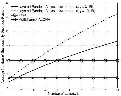
(a)

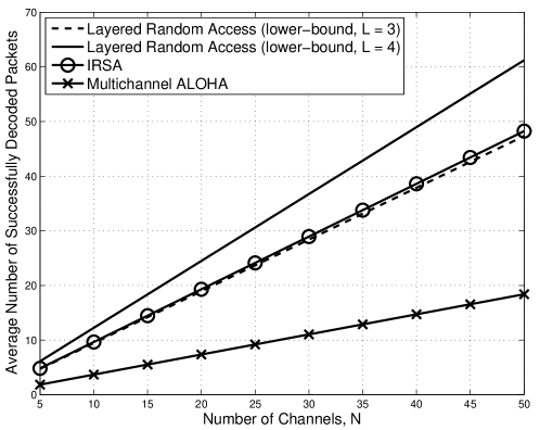
(b)

Figure 2: Comparisons between the proposed layered random access scheme, IRSA, and multichannel ALOHA in terms of the average number of successfully decoded packets: (a) the average number of successfully decoded packets versus $L$ with $N=10$; (b) the average number of successfully decoded packets versus $N$ with $\gamma=10$ dB and $L\in\{3,4\}$.

Note that the comparisons in Fig. 2 may not be complete as no fading is considered for IRSA and multichannel ALOHA, while the results in Fig. 2 might be favorable to IRSA and multichannel ALOHA (as no fading is considered for them). In addition, it is noteworthy that the proposed layered random access scheme can exploit the notion of IRSA within each layer with iterative decoding. In this case, a receiver can employ not only inter-layer, but also intra-layer SIC. This generalization might be a further research topic to be studied in the future.

IV Random CRRD for Reliable Transmissions with a Delay Constraint

In the previous sections, we have considered the layered random access scheme that can improve the throughput. This scheme can be modified to guarantee successful packet delivery within a slot with a sufficiently high probability. To this end, we can consider random CRRD where a packet from a user is to be transmitted through randomly selected multiple channels.

Throughout this section, we consider the following assumption that replaces A2.

• A user can transmit $B$ copies of a packet through randomly selected $B$ channels out of $N$ channels, where $B\leq N$, in a randomly (and uniformly) selected layer. To avoid self-packet collision, a user is to choose $B$ different channels. Each copy of a packet has the pointers of the other $B-1$ copies as in [11] so that any successfully decoded copy can help remove the other copies by interference cancellation.

For convenience, $B$ is referred to as the repetition gain. Clearly, if $B=N$, the resulting random access is identical to single-channel ALOHA with $N$-fold transmit diversity, which can be seen as a generalization of [25]. Under the assumption of A5, provided that there are $m$ active users in a layer, the conditional probability of collision becomes

$$p_{\rm c}(m)=1-\left(1-\frac{1}{N}\right)^{B(m-1)},$$ (24)

which can be seen a generalization of (5), as (24) becomes (5) with $B=1$. Let ${\cal B}_{k,l}$ denote the index set of the selected $B$ channels by user $k$ provided that user $k$ chooses layer $l$. The conditional probability of collision or decoding error of the signal transmitted by a user through channel $q\in{\cal B}_{k,l}$, provided that there are $m$ transmitted signals in layer $l$, becomes

$$\alpha_{l}(m)=p_{\rm c}(m)+(1-p_{\rm c}(m))\beta_{l},$$ (25)

where $\beta_{l}$ is the conditional probability of decoding error of layer $l$ with only one signal from user $k$ at channel $q$ under the lower-interference-free condition for layer $l$ and the assumption of A5. Note that $p_{\rm c}(m)$, $\alpha_{l}(m)$, and $\beta_{l}$ are slightly different from those in the previous sections due to multiple transmissions (or the assumption of A5). However, as long as there is no risk of confusion, we will use the same notations in this section.

Since there are $B$ copies, under the assumption of A3, the conditional probability of collision or decoding error becomes $\alpha_{l}^{B}(m)$ if the signals in channels are independent. Thus, the (conditional) probability of collision or decoding error of a user’s signal in layer $l$ under the lower-interference-free condition is given by

$$\Psi_{l}=\sum_{m=1}^{\infty}\alpha_{l}^{B}(m)\bar{P}_{l}(m),$$ (26)

where

$$\bar{P}_{l}(m_{l})=\Pr(m_{l}\,|\,m_{l}\geq 1)=\frac{P_{l}(m)}{1-e^{-\lambda_{l}}},\ m_{l}=1,\ldots.$$ (27)

Here, $m_{l}$ represents the number of active users at layer $l$. Clearly, if $B$ is large, $\alpha_{l}^{B}(m)$ is small, which can result in a low probability of collision or decoding error. Thus, for a large $B$, a successful packet transmission subject to the delay constraint to transmit within one slot or a MAC frame can be guaranteed with a high probability for reliable low latency transmissions at the cost of throughput. However, due to multiple layers, it might be possible to transmit more packets within a slot.

In fact, (26) is valid only if the $\sigma_{l,q}^{2}$’s, $q\in{\cal B}_{k,l}$, are independent. However, since each active user sends $B$ copies of signals to $B$ different channels, $\sigma_{l,q}^{2}$ and $\sigma_{l,q^{\prime}}^{2}$ can be correlated if any active user in layer $i\in\{l+1,\ldots,L\}$ sends his/her signal to channels $q$ and $q^{\prime}$ too. As a result, (26) is an approximation unless $B=1$. In general, if $B\ll N$, (26) might be a reasonably good approximation.

Lemma 4

Under the assumptions of A1, A3, A4, and A5, the approximation of $\Psi_{l}$ can be expressed by a sum of finite terms as follows:

$$\Psi_{l} \approx\sum_{m=1}^{\infty}\alpha_{l}^{B}(m)\bar{P}_{l}(m)$$ (28)

$$=\sum_{b=0}^{B}\binom{B}{b}(1-\beta_{l})^{b}\beta_{l}^{B-b}g_{l}(b),$$ (29)

where

$$g_{l}(b) =\frac{e^{-\lambda_{l}}}{1-e^{-\lambda_{l}}}\sum_{j=0}^{b}\binom{b}{j}(-\omega)^{-j}(e^{\lambda_{l}\omega^{j}}-1)$$ (30)

$$\beta_{l} =1-e^{-\frac{\nu(R_{l})N_{0}}{P_{l}\sigma_{h}^{2}}-\sum_{i=l+1}^{L}\frac{\lambda_{i}B}{N}\frac{\nu(R_{l})P_{i}}{P_{l}+\nu(R_{l})P_{i}}}.$$ (31)

Here, $\omega=\left(1-\frac{1}{N}\right)^{B}$.

Proof:

See Appendix C. ∎

From the $\Psi_{l}$’s, we can define the outage probability of each layer as the probability that any of $B$ copied packets from a user cannot be successfully decoded at layer $l$. The outage probability of layer 1 is equal to $\Psi_{1}$. For layer $l$, $l>1$, by taking into account the error propagation, we have

$$P_{{\rm out},l}=1-\prod_{i=1}^{l}(1-\Psi_{i}).$$ (32)

Due to the closed-form expression in (29), the outage probability can be found in a closed-form, which can help optimize key parameters such as $B$ to minimize the outage probability. Note that if $\Psi_{l}\ll\Psi_{1}$ for $l=2,\ldots,L$, we can see that the outage probability is generally decided by $\Psi_{1}$ or $P_{{\rm out},1}$. For a low $\Psi_{1}$, we expect to have reliable transmissions within a slot. Furthermore, since $P_{{\rm out},l}$ increases with $l$, the users who can accept tolerable reliability can choose upper layers, i.e., layers $l\in\{2,\ldots,L\}$.

Note that unlike IRSA, no intra-layer SIC is used in the modified layered scheme with CRRD in this section. Furthermore, as no iterative decoding is used, the processing delay at a receiver is fixed, which is desirable for high reliability low latency communications.

V Simulation Results

In this section, we present simulation results to see the performance of the proposed layered random access scheme Rayleigh fading in terms of the throughput (without CRRD) and outage probability (with CRRD).

V-A Throughput

In this subsection, we present simulation results under the assumptions of A1 – A4. For simulations, we assume that the transmit powers are decided as in (21) and $\sigma_{h}^{2}=N_{0}=1$ for normalization. In addition, for convenience, we assume that $\lambda=\lambda_{l}$, $l=1,\ldots,L$ (i.e., an equal arrival rate is assumed for all the layers). The throughput in this section is in the number of bits per channel use as mentioned earlier.

Fig. 3 presents the throughput of the layered random access scheme for different arrival rate, $\lambda$, when $N=10$ and $\gamma=3$ dB. In Fig. 3 (a), with $L=3$, the throughput of each layer is shown with the optimal rates that are found from (19) for each value of $\lambda$. We can see that the theoretical result agrees with the simulation result for layer $1$. However, we find that the theoretical result becomes an approximation for the bottom layers, i.e., layers 2 and 3 due to the correlation of the events of successful decoding in different layers as explained earlier. From this, the theoretical total throughput becomes an approximation as in Fig. 3 (b), where we can also observe that the total throughput is improved with more layers. In Fig. 3 (b), we can also observe that the arrival rate per layer that maximizes the throughput is less than the number of channels, $N$, and decreases with the number of layers. In order to avoid frequent collisions, an arrival rate lower than $N$ might be desirable (which could result in a higher throughput). In addition, since the interference power increases with the number of layers, the arrival rate can decrease with the number of layers for a reasonable interference power and to achieve a higher throughput.

Fig. 4 shows that the transmit power increases with the number of layers. From this, we can see that the total throughput is improved at the cost of higher transmit power. In addition, the transmit power increases with $\lambda$ to meet the nominal SINR because the interference power increases with $\lambda$ (which is shown in (16)).

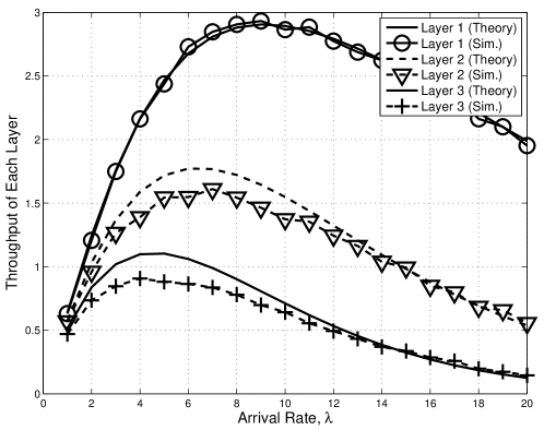
(a)

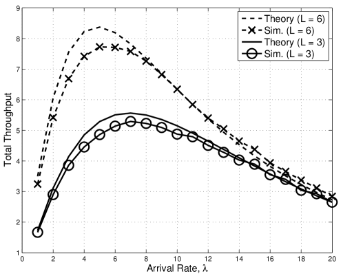
(b)

Figure 3: Throughput versus arrival rate $\lambda$ with $\gamma=3$ dB and $N=10$: (a) throughput of each layer; (b) total throughput with $L=3$ and $L=6$.

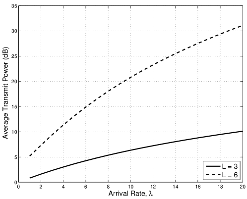
Figure 4: Average transmit power for different arrival rate, $\lambda$ with $\gamma=3$ dB, $L\in\{3,6\}$, and $N=10$.

In Fig. 5, we assume an equal transmission rate for all the layers, i.e., $R=R_{l}$, $l=1,\ldots,L$, and show the total throughput for different values of $R$ when $N=10$, $\lambda=N$, $L\in\{3,6\}$, and $\gamma=3$ dB. We can observe that the optimal rates that are obtained from (19) can provide the best performance in terms of the total throughput.

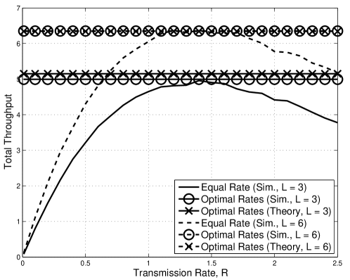
Figure 5: Total throughput for different transmission rate, $R=R_{l}$, $l=1,\ldots,L$, when $N=10$, $\lambda=N$, $L\in\{3,6\}$, and $\gamma=3$ dB.

In Fig. 6, we show the total throughput for different target SNR, $\gamma$, when $N=10$, $\lambda=N$, and $L\in\{3,6\}$. Since $\varphi_{l}$ increases with $\gamma$, the total throughput increases with $\gamma$ as shown in Fig. 6.

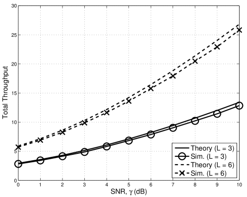
Figure 6: Total throughput for different target SNR, $\gamma$, when $N=10$, $\lambda=N$, and $L\in\{3,6\}$.

Fig. 7 shows the total throughput for different numbers of layers, $L$, when $N=10$, $\lambda\in\{N/2,N\}$, and $\gamma=3$ dB. The total throughput increases with $L$, while it becomes saturated for a large $L$. In particular, when $\lambda=N$, the total throughput slowly increases with $L$ when $L\geq 4$. Interestingly, for a large $L$ (e.g., 8), we can observe that the total throughput can be higher with a lower arrival rate $\lambda$. This shows that a lower arrival rate is desirable for a larger number of layers to keep the interference low, which may result in a higher total throughput.

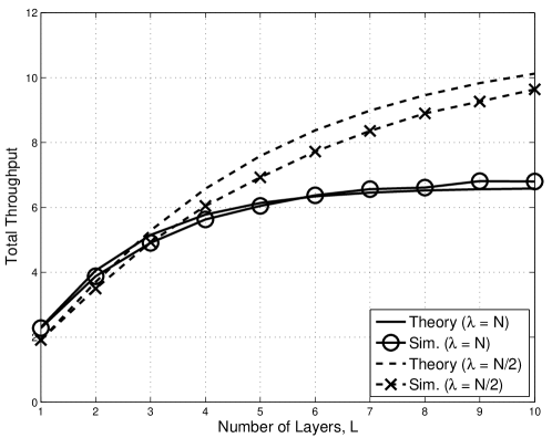
Figure 7: Total throughput for different numbers of layers, $L$, when $N=10$, $\lambda\in\{N/2,N\}$, and $\gamma=3$ dB.

V-B Outage Probability

In this subsection, we present simulation results when each user transmits $B$ copies of a packet through different channels for reliable transmissions (i.e., with CRRD). We show the outage probabilities that are obtained by the theoretical approximations (i.e., (29) and (32)) and simulations under the assumptions of A1, A3, A4, and A5 with $\sigma_{h}^{2}=N_{0}=1$. Furthermore, throughout this subsection, we assume that $R=R_{l}$ and $\lambda=\lambda_{l}$, $l=1,\ldots,L$, while the powers are decided as in (21).

Fig. 8 shows the outage probability for different values of transmission rate, $R$, when $B=4$, $N=60$, $L=3$, $\lambda=3$, and $\gamma=10$ dB. Clearly, we can see a trade-off relationship between the transmission rate and reliability with a delay constraint. That is, we can achieve reliable transmissions with a delay constraint at the cost of transmission rates. We can also see that although (32) is an approximation, it can provide reasonably good approximations of the outage probabilities at around $R=1$.

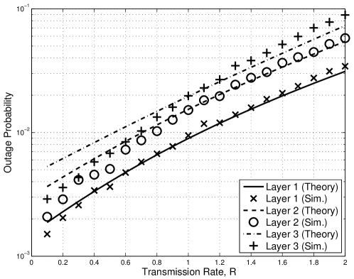
Figure 8: Outage probabilities for different values of transmission rate, $R$, when $B=4$, $N=60$, $L=3$, $\lambda=3$, and $\gamma=10$ dB.

In Fig. 9, we present the outage probability for different values of repetition gain, $B$, when $R=1$, $N=60$, $L=3$, $\lambda=3$, and $\gamma=10$ dB. It is interesting to see that there might be an optimal $B$, which is around 6. If $B$ is too large, there might be more collisions. On the other hand, if $B$ is too small, the multiple transmit diversity gain is small. Note that there is a noticeable gap between the theoretical approximations and simulation results for a large $B$, because (29) is obtained without taking into account the correlation of the $\sigma_{l,q}^{2}$’s that increases with $B$.

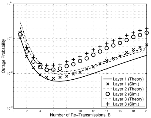
Figure 9: Outage probabilities for different values of repetition gain, $B$, when $R=1$, $N=60$, $L=3$, $\lambda=3$, and $\gamma=10$ dB.

In Fig. 10, the outage probabilities are shown for different values of arrival rate, $\lambda$, when $B=4$, $N=60$, $L=3$, $R=1$, and $\gamma=10$ dB. For a low outage probability, it is desirable to have a low arrival rate, $\lambda$. This might be seen as a trade-off relationship between the throughput and reliability with a delay constraint. Together with the results in Fig. 9, we can conclude that reliable transmissions with a delay constraint can be achieved with CRRD at the cost of transmission rates as well as arrival rates or throughput.

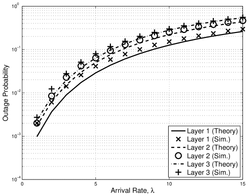
Figure 10: Outage probabilities for different values of arrival rate, $\lambda$, when $B=4$, $N=60$, $L=3$, $R=1$, and $\gamma=10$ dB.

From Figs. 8 – 10, we can see that the outage probabilities of layers are not significantly different, while the outage probability increases with $l$ as expected. With a large $L$, we can have more transmissions. However, the users choosing upper layers, i.e., a large $l$, should be more tolerable for transmission reliability.

VI Concluding Remarks

We considered a layered random access scheme that can support more users by exploiting the notion of NOMA in this paper. To find the throughput, we derived a closed-form expression for the probability of successful decoding by taking into account packet collision as well as decoding errors due to low instantaneous SINR. From this, a closed-form expression for the total throughput was derived. Although it is an approximation as the correlation of the events of successful decoding in different layers has been ignored, it allowed us to find optimal rates that maximize the total throughput. From simulation results, we confirmed that the resulting optimal rates can provide the highest throughput (as shown in Fig. 5).

From brief comparisons between the proposed layered random access scheme and IRSA, we found that the proposed layered random access scheme can provide a higher throughput using multiple layers than IRSA. A generalization of the proposed scheme with the notion of IRSA might be an interesting topic where a receiver can employ not only inter-layer, but also intra-layer SIC. This generalization might be a further research topic to be studied in the future.

We also modified the proposed layered random access scheme with CRRD so that a receiver can decode the signals from users within a slot (or MAC frame) with a high probability. A closed-form expression for the outage probability is derived, which is an approximation and reasonably good when the repetition gain is not too large. From simulation results and analysis, we observed that reliable transmissions can be accomplished with a high probability at the cost of transmission rates as well as arrival rates or throughput.

Appendix A Proof of Lemma 1

From (4), we have

$$\eta_{l} =\sum_{m=0}^{\infty}m(1-\alpha_{1}(m))P_{l}(m)$$ (33)

$$=(1-\beta_{l})\sum_{m=0}^{\infty}m(1-p_{\rm c}(m))P_{l}(m),$$ (34)

where $P_{l}(m)$ is the probability that there are $m$ active users at layer $l$. Under the assumption of A1, since $P_{l}(m)=\frac{\lambda_{l}^{m}e^{-\lambda_{l}}}{m!}$, it follows

$$\eta_{l} =(1-\beta_{l})\lambda_{l}\sum_{m=1}^{\infty}\left(1-\frac{1}{N}\right)^{m-1}\frac{\lambda_{l}^{m-1}e^{-\lambda_{l}}}{(m-1)!}$$ (35)

$$=\varphi_{l}\lambda_{l}e^{\lambda_{l}\left(1-\frac{1}{N}\right)}e^{-\lambda_{l}},$$ (36)

which leads to (6). This completes the proof.

Appendix B Proof of Lemma 2

Under the assumption of A4, $|h_{k,q}|^{2}$ becomes an independent chi-squared random variable with 2 degrees of freedom. Let $D_{l,q}$ denote the number of users transmitting signals through channel $q$ and layer $l$. Then, $\sigma_{l,q}^{2}$ can be given by

$$\sigma_{l,q}^{2} ={\mathbb{E}}[|n_{l,q}|^{2}\,|\,\{h_{k,q}\}]$$ (37)

$$=\sum_{i=l+1}^{L}P_{i}\sum_{k\in{\cal I}_{i,q}}|h_{k,q}|^{2}+N_{0}$$ (38)

$$=\sum_{i=l+1}^{L}\frac{\sigma_{h}^{2}P_{i}}{2}\chi_{2D_{i,q}}^{2}+N_{0},$$ (39)

where $\chi_{2D}^{2}$ represents an independent chi-squared random variable with $2D$ degrees of freedom. Under the assumptions of A1 and A2, we can see that $D_{l,q}$ is an independent Poisson random variable with mean $\frac{\lambda_{l}}{N}$. Thus, it can be shown that

$${\mathbb{E}}\left[\frac{\sigma_{h}^{2}P_{i}}{2}\chi_{2D_{i,q}}^{2}\right]=\frac{\sigma_{h}^{2}P_{i}\lambda_{i}}{N}.$$ (40)

Under the assumption of A4, from (3), the decoding error probability becomes

$$\beta_{l}=1-{\mathbb{E}}\left[\exp\left(-\frac{\sigma_{l}^{2}\nu(R_{l})}{P_{l}\sigma_{h}^{2}}\right)\right].$$ (41)

Then, using Jensen’s inequality, we have

$$\varphi_{l}\geq\exp\left(-\frac{{\mathbb{E}}[\sigma_{l}^{2}]\nu(2^{R_{l}})}{P_{l}\sigma_{h}^{2}}\right)=\exp\left(-\frac{\nu(R_{l})}{\gamma_{l}}\right),$$ (42)

which becomes the lower-bound in (15).

To find the exact expression, from (41), we have

$$\varphi_{l} =e^{-\frac{\nu(R_{l})N_{0}}{P_{l}\sigma_{h}^{2}}}{\mathbb{E}}\left[e^{-\frac{\nu(R_{l})}{P_{l}}\sum_{i=l+1}^{L}\frac{P_{i}\chi_{2D_{i,q}}^{2}}{2}}\right].$$ (43)

Since $\chi_{2D}^{2}$ is a chi-squared random variable (under the assumption of A4), it can be shown that

$${\mathbb{E}}\left[e^{-\frac{\nu(R_{l})}{P_{l}}\sum_{i=l+1}^{L}\frac{P_{i}\chi_{2D_{i,q}}^{2}}{2}}\right] =\prod_{i=l+1}^{L}{\mathbb{E}}\left[e^{-\frac{\nu(R_{l})}{P_{l}}\frac{P_{i}\chi_{2D_{i,q}}^{2}}{2}}\right]$$ (44)

$$=\prod_{i=l+1}^{L}{\mathbb{E}}\left[\left(\frac{1}{1+\frac{\nu(R_{l})P_{i}}{P_{l}}}\right)^{D_{i,q}}\right].$$ (45)

Now, noting that $D_{i,q}$ is a Poisson random variable (under the assumptions of A1 and A2), we have

$${\mathbb{E}}\left[\left(\frac{1}{1+\frac{\nu(R_{l})P_{i}}{P_{l}}}\right)^{D_{i,q}}\right]$$ (46)

$$=\sum_{d=0}^{\infty}\left(\frac{1}{1+\frac{\nu(R_{l})P_{i}}{P_{l}}}\right)^{d}\frac{(\lambda_{i}/N)^{d}}{d!}e^{-\lambda_{i}/N}$$ (47)

$$=\exp\left(-\frac{\lambda_{i}}{N}\frac{\nu(R_{l})P_{i}}{P_{l}+\nu(R_{l})P_{i}}\right).$$ (48)

Substituting (48) into (45), we have

$${\mathbb{E}}\left[e^{-\frac{\nu(R_{l})}{P_{l}}\sum_{i=l+1}^{L}\frac{P_{i}\chi_{2D_{i,q}}^{2}}{2}}\right]=e^{-\sum_{i=l+1}^{L}\frac{\lambda_{i}}{N}\frac{\nu(R_{l})P_{i}}{P_{l}+\nu(R_{l})P_{i}}}.$$ (49)

Finally, substituting (49) to (43), we can obtain the exact expression in (15).

Appendix C Proof of Lemma 4

It can be shown that

$$\sum_{m=1}^{\infty}\alpha_{l}^{B}(m)\bar{P}_{l}(m)$$ (50)

$$=\sum_{m=1}^{\infty}\left(p_{\rm c}(m)+(1-p_{\rm c}(m))\beta_{l}\right)^{B}\bar{P}_{l}(m)$$ (51)

$$=\sum_{m=1}^{\infty}\sum_{b=0}^{B}\binom{B}{b}(1-\beta_{l})^{b}p_{\rm c}^{b}(m)\beta_{l}^{B-b}\bar{P}_{l}(m)$$ (52)

$$=\sum_{b=0}^{B}\binom{B}{b}(1-\beta_{l})^{b}\beta_{l}^{B-b}\sum_{m=1}^{\infty}p_{\rm c}^{b}(m)\bar{P}_{l}(m).$$ (53)

In order to find an expression with a sum of finite terms, we can show that

$$\sum_{m=1}^{\infty}p_{\rm c}^{b}(m)\bar{P}_{l}(m) =\sum_{m=1}^{\infty}(1-\omega^{m-1})^{b}P_{l}(m)$$

$$=\sum_{j=0}^{b}\binom{b}{j}\sum_{m=1}^{\infty}(-\omega^{m-1})^{j}\bar{P}_{l}(m)$$

$$=\frac{e^{-\lambda_{l}}}{1-e^{-\lambda_{l}}}\sum_{j=0}^{b}\binom{b}{j}(-\omega)^{-j}(e^{\lambda_{l}\omega^{j}}-1).$$

Substituting (C) into (53), we have

$$\Psi_{l} \approx\frac{e^{-\lambda_{l}}}{1-e^{-\lambda_{l}}}\sum_{b=0}^{B}\binom{B}{b}(1-\beta_{l})^{b}\beta_{l}^{B-b}$$ (54)

$$\times\sum_{j=0}^{b}\binom{b}{j}(-\omega)^{-j}(e^{\lambda_{l}\omega^{j}}-1),$$ (55)

which is (29).

Note that $\beta_{l}$ in (31) is different from $1-\varphi_{l}$ that can be obtained from (15) due to multiple transmissions (i.e., $B>1$). Under the assumptions of A1 and A5, $D_{i,q}$ in (39) is a Poisson random variable with mean $\frac{\lambda_{i}B}{N}$ instead of $\frac{\lambda_{i}}{N}$, i.e., $D_{i,q}\sim{\rm Poiss}\left(\frac{B\lambda_{i}}{N}\right)$. Thus, under the assumption of A4, we have

$${\mathbb{E}}\left[e^{-\frac{\nu(R_{l})}{P_{l}}\sum_{i=l+1}^{L}\frac{P_{i}\chi_{2D_{i,q}}^{2}}{2}}\right]=e^{-\sum_{i=l+1}^{L}\frac{\lambda_{i}B}{N}\frac{\nu(R_{l})P_{i}}{P_{l}+\nu(R_{l})P_{i}}},$$ (56)

which is substituted into (43) to obtain $\beta_{l}$ in (31).

References

- [1] 3GPP TR 37.868 V11.0, Study on RAN improvments for machine-type communications, October 2011.
- [2] 3GPP TS 36.321 V13.2.0, Evolved Universal Terrestrial Radio Access (E-UTRA); Medium Access Control (MAC) protocol specification, June 2016.
- [3] N. Abramson, “THE ALOHA SYSTEM: Another alternative for computer communications,” in Proceedings of the November 17-19, 1970, Fall Joint Computer Conference, AFIPS ’70 (Fall), (New York, NY, USA), pp. 281–285, ACM, 1970.
- [4] B. Bertsekas and R. Gallager, Data Networks. Englewood Cliffs: Prentice-Hall, 1987.
- [5] D. Shen and V. O. K. Li, “Performance analysis for a stabilized multi-channel slotted ALOHA algorithm,” in Proc. IEEE PIMRC, vol. 1, pp. 249–253 Vol.1, Sept 2003.
- [6] O. Arouk and A. Ksentini, “Multi-channel slotted aloha optimization for machine-type-communication,” in Proc. of the 17th ACM International Conference on Modeling, Analysis and Simulation of Wireless and Mobile Systems, pp. 119–125, 2014.
- [7] C. H. Chang and R. Y. Chang, “Design and analysis of multichannel slotted ALOHA for machine-to-machine communication,” in Proc. IEEE GLOBECOM, pp. 1–6, Dec 2015.
- [8] J. Choi, “On the adaptive determination of the number of preambles in RACH for MTC,” IEEE Communications Letters, vol. 20, pp. 1385–1388, July 2016.
- [9] Y. Yu and G. B. Giannakis, “High-throughput random access using successive interference cancellation in a tree algorithm,” IEEE Trans. Information Theory, vol. 53, pp. 4628–4639, Dec 2007.
- [10] E. Casini, R. D. Gaudenzi, and O. D. R. Herrero, “Contention resolution diversity slotted aloha (CRDSA): An enhanced random access schemefor satellite access packet networks,” IEEE Trans. Wireless Communications, vol. 6, pp. 1408–1419, April 2007.
- [11] G. Liva, “Graph-based analysis and optimization of contention resolution diversity slotted ALOHA,” IEEE Trans. Communications, vol. 59, pp. 477–487, February 2011.
- [12] E. Paolini, G. Liva, and M. Chiani, “Coded slotted ALOHA: A graph-based method for uncoordinated multiple access,” IEEE Trans. Information Theory, vol. 61, pp. 6815–6832, Dec 2015.
- [13] E. Paolini, C. Stefanovic, G. Liva, and P. Popovski, “Coded random access: applying codes on graphs to design random access protocols,” IEEE Communications Magazine, vol. 53, pp. 144–150, June 2015.
- [14] J. Choi, “Non-orthogonal multiple access in downlink coordinated two-point systems,” IEEE Commun. Letters, vol. 18, pp. 313–316, Feb. 2014.
- [15] Z. Ding, Z. Yang, P. Fan, and H. Poor, “On the performance of non-orthogonal multiple access in 5G systems with randomly deployed users,” IEEE Signal Process. Letters, vol. 21, pp. 1501–1505, Dec 2014.
- [16] Z. Ding, Y. Liu, J. Choi, M. Elkashlan, C. L. I, and H. V. Poor, “Application of non-orthogonal multiple access in LTE and 5G networks,” IEEE Communications Magazine, vol. 55, pp. 185–191, February 2017.
- [17] J. Choi, “NOMA based random access with multichannel ALOHA,” IEEE J. Selected Areas in Communications, (to appear).
- [18] Y. Liang, X. Li, J. Zhang, and Z. Ding, “Non-orthogonal random access for 5G networks,” IEEE Trans. Wireless Communications, vol. 16, pp. 4817–4831, July 2017.
- [19] N. Zhang, J. Wang, G. Kang, and Y. Liu, “Uplink nonorthogonal multiple access in 5G systems,” IEEE Communications Letters, vol. 20, pp. 458–461, March 2016.
- [20] D. J. Goodman and A. A. M. Saleh, “The near/far effect in local ALOHA radio communications,” IEEE Trans. Vehicular Technology, vol. 36, pp. 19–27, Feb 1987.
- [21] M. Zorzi, “Capture probabilities in random-access mobile communications in the presence of rician fading,” IEEE Trans. Vehicular Technology, vol. 46, pp. 96–101, Feb 1997.
- [22] N. A. Johansson, Y. P. E. Wang, E. Eriksson, and M. Hessler, “Radio access for ultra-reliable and low-latency 5G communications,” in 2015 IEEE International Conference on Communication Workshop (ICCW), pp. 1184–1189, June 2015.
- [23] G. Durisi, T. Koch, and P. Popovski, “Toward massive, ultrareliable, and low-latency wireless communication with short packets,” Proceedings of the IEEE, vol. 104, pp. 1711–1726, Sept 2016.
- [24] D. Tse and P. Viswanath, Fundamentals of Wireless Communication. Cambridge University Press, 2005.
- [25] G. Choudhury and S. Rappaport, “Diversity ALOHA - a random access scheme for satellite communications,” IEEE Trans. Communications, vol. 31, pp. 450–457, March 1983.