A Superconvergent Hybridizable Discontinuous Galerkin Method for Dirichlet Boundary Control of Elliptic PDEs

Abstract

We begin an investigation of hybridizable discontinuous Galerkin (HDG) methods for approximating the solution of Dirichlet boundary control problems governed by elliptic PDEs. These problems can involve atypical variational formulations, and often have solutions with low regularity on polyhedral domains. These issues can provide challenges for numerical methods and the associated numerical analysis. We propose an HDG method for a Dirichlet boundary control problem for the Poisson equation, and obtain optimal a priori error estimates for the control. Specifically, under certain assumptions, for a 2D convex polygonal domain we show the control converges at a superlinear rate. We present 2D and 3D numerical experiments to demonstrate our theoretical results.

1 Introduction

We consider the following elliptic Dirichlet boundary control problem on a Lipschitz polyhedral domain $\Omega\subset\mathbb{R}^{d}$, $d\geq 2$, with boundary $\Gamma=\partial\Omega:$

$$\min J(u),\quad J(u)=\frac{1}{2}\|y-y_{d}\|^{2}_{L^{2}(\Omega)}+\frac{\gamma}{2}\|u\|^{2}_{L^{2}(\Gamma)},$$ (1)

where $\gamma>0$ and $y$ is the solution of the Poisson equation with nonhomogeneous Dirichlet boundary conditions

$$-\Delta y =f\quad\text{in}\;\Omega,$$ (2)

$$y =u\quad\text{on}\;\Gamma.$$ (3)

It is well known that the Dirichlet boundary control problem (1)-(3) is equivalent to the optimality system

$$-\Delta y =f\quad\quad\quad\;\text{in}\;\Omega,$$ (4a)

$$y =u\quad\quad\quad\;\text{on}\;\Gamma,$$ (4b)

$$-\Delta z =y-y_{d}\quad\;\text{in}\;\Omega,$$ (4c)

$$z =0\quad\quad\quad\;\;\text{on}\;\Gamma,$$ (4d)

$$u =\gamma^{-1}\frac{\partial z}{\partial\bm{n}}\quad\text{on}\;\Gamma.$$ (4e)

where $\bm{n}$ is the unit outer normal to $\Gamma$.

Dirichlet boundary control has many applications in fluid flow problems and other fields, and therefore the mathematical study of these control problems has become an important area of research. Major theoretical and computational developments have been made in the recent past; see, e.g., [26, 25, 19, 20, 24, 21, 16, 45, 42, 27, 17, 43, 7]. However, only in the last ten years have researchers developed thorough well-posedness, regularity, and finite element error analysis results for elliptic PDEs; see [5, 18, 33, 46, 1] and the references therein. One difficulty of Dirichlet boundary control problems is that the Dirichlet boundary data does not directly enter a standard variational setting for the PDE; instead, the state equation is understood in a very weak sense. Also, solutions of the optimality system typically do not have high regularity on polyhedral domains; corners cause the normal derivative of the adjoint state $\partial z/\partial\bm{n}$ in the optimality condition (4) to have limited smoothness. Solutions with limited regularity can lead to complications for numerical methods and numerical analysis.

To avoid the difficulties described above, researchers have considered other approaches including modified cost functionals [39, 23, 25, 11], approximating the Dirichlet boundary condition with a Robin boundary condition [2, 3, 4, 28, 41], and weak boundary penalization [8].

One way to approximate the solution of the original problem without penalization and also avoid the variational difficulty is to use a mixed finite element method. Recently, Gong and Yan [22] considered this approach and obtained

$$\left\lVert u-u_{h}\right\rVert_{0,\Omega}=O(h^{1-1/s})$$

when the control belongs to $H^{1-1/s}(\Gamma)$ and the lowest order Raviart-Thomas elements are used for the computation.

As researchers continue to investigate Dirichlet boundary control problems of increasingly complexity, it may become natural to utilize discontinuous Galerkin methods for the spatial discretization of problems involving strong convection and discontinuities. We have performed preliminary computations using an hybridizable discontinuous Galerkin (HDG) method for a similar elliptic Dirichlet boundary control problem for the Stokes equations. Our preliminary results for this problem indicate that the optimal control can indeed be discontinuous at the corners of the domain. Before we continue to investigate problems of such complexity, we begin this line of research by considering an HDG method to approximate the solution of the above Dirichlet boundary control problem.

HDG methods also utilize a mixed formulation and therefore avoid the variational difficulty of the Dirichlet control problem. Furthermore, the number of degrees of freedom for HDG methods are much less than standard mixed methods or other DG approaches. Moreover, the RT element is a special case of the HDG method. We provide more background about HDG methods in Section 3.

We propose an HDG method to approximate the control in Section 3, and in Section 4 we prove an optimal superlinear rate of convergence for the control in 2D under certain assumptions on the domain and $y_{d}$. To give a specific example, for a rectangular 2D domain and $y_{d}\in H^{1}(\Omega)\cap L^{\infty}(\Omega)$, we obtain the following a priori error bounds for the state $y$, adjoint state $z$, their fluxes $\bm{q}=-\nabla y$ and $\bm{p}=-\nabla z$, and the optimal control $u$:

$$\left\lVert y-{y}_{h}\right\rVert_{0,\Omega}=O(h^{3/2-\varepsilon}),\quad\;\left\lVert z-{z}_{h}\right\rVert_{0,\Omega}=O(h^{3/2-\varepsilon}),$$

$$\left\lVert\bm{q}-\bm{q}_{h}\right\rVert_{0,\Omega}=O(h^{1-\varepsilon}),\quad\quad\;\;\left\lVert\bm{p}-\bm{p}_{h}\right\rVert_{0,\Omega}=O(h^{3/2-\varepsilon}),$$

and

$$\left\lVert u-{u}_{h}\right\rVert_{0,\Gamma}=O(h^{3/2-\varepsilon}),$$

for any $\varepsilon>0$. We demonstrate the performance of the HDG method with numerical experiments in 2D and 3D in Section 5.

2 Background: The Optimality System and Regularity

To begin, we review some fundamental results concerning the optimality system for the control problem and the regularity of the solution in 2D polygonal domains.

Throughout the paper we adopt the standard notation $W^{m,p}(\Omega)$ for Sobolev spaces on $\Omega$ with norm $\|\cdot\|_{m,p,\Omega}$ and seminorm $|\cdot|_{m,p,\Omega}$ . We denote $W^{m,2}(\Omega)$ by $H^{m}(\Omega)$ with norm $\|\cdot\|_{m,\Omega}$ and seminorm $|\cdot|_{m,\Omega}$. Also, $H_{0}^{1}(\Omega)=\{v\in H^{1}(\Omega):v=0\;\mbox{on}\;\partial\Omega\}$. We denote the $L^{2}$-inner products on $L^{2}(\Omega)$ and $L^{2}(\Gamma)$ by

$$(v,w) =\int_{\Omega}vw\quad\forall v,w\in L^{2}(\Omega),$$

$$\left\langle v,w\right\rangle =\int_{\Gamma}vw\quad\forall v,w\in L^{2}(\Gamma).$$

Define the space $H(\text{div};\Omega)$ as

$$H(\text{div},\Omega)=\{\bm{v}\in[L^{2}(\Omega)]^{2},\nabla\cdot\bm{v}\in L^{2}(\Omega)\}.$$

To avoid the the variational difficulty we follow the strategy introduced by Wei Gong and Ningning Yan [22] and consider a mixed formulation of the optimality system. Introduce two flux variables $\bm{q}=-\nabla y$ and $\bm{p}=-\nabla z$. The mixed weak form of (4a)-(4e) is

$$(\bm{q},\bm{r})-(y,\nabla\cdot\bm{r})+\left\langle u,\bm{r}\cdot\bm{n}\right\rangle =0,$$ (5a)

$$(\nabla\cdot\bm{q},w) =(f,w),$$ (5b)

$$(\bm{p},\bm{r})-(z,\nabla\cdot\bm{r}) =0,$$ (5c)

$$(\nabla\cdot\bm{p},w)-(y,w) =(y_{d},w),$$ (5d)

$$\left\langle\gamma u+\bm{p}\cdot\bm{n},\xi\right\rangle =0,$$ (5e)

for all $(\bm{r},w,\xi)\in H(\text{div},\Omega)\times L^{2}(\Omega)\times L^{2}(\Gamma)$.

One of the main reasons that Dirichlet boundary control problem can be challenging numerically is that the solution can have very low regularity, and this restricts the convergence rates of finite element and DG methods. In order to prove a superlinear convergence rate for the optimal control for the HDG method in 4, we assume the solution has the following fractional Sobolev regularity:

$$u\in H^{r_{u}}(\Gamma),\quad y\in H^{r_{y}}(\Omega),\quad z\in H^{r_{z}}(\Omega),\quad\bm{q}\in H^{r_{\bm{q}}}(\Omega),\quad\bm{p}\in H^{r_{\bm{p}}}(\Omega),$$ (6)

with

$$r_{u}>1,\quad r_{y}>1,\quad r_{z}>2,\quad r_{\bm{q}}>1/2,\quad r_{\bm{p}}>1.$$ (7)

We require $r_{\bm{q}}>1/2$ in order to guarantee $q$ has a well-defined trace on the boundary $\Gamma$. We note that it may be possible to use the techniques in [30] to lower the regularity requirement on $\bm{q}$. We leave this to be considered elsewhere.

For a 2D convex polygonal domain and $f=0$, we use a recent regularity result of Mateos and Neitzel [32] below to give conditions on the domain and $y_{d}$ to guarantee the solution has the above regularity. For a higher dimensional convex polyhedral domain, the regularity theory is much more complicated, and we do not attempt to provide conditions to guarantee the above regularity in this work.

Theorem 1 ([32], Lemma 3 and Corollary 1).

Suppose $f=0$ and $\Omega\subset\mathbb{R}^{2}$ is a bounded convex domain with polygonal boundary $\Gamma$. Let $\omega\in[\pi/3,\pi)$ be the largest interior angle of $\Gamma$, and define $p_{\Omega}$, $r_{\Omega}$ by

$$p_{\Omega}=\frac{2}{2-\pi/\max\{\omega,\pi/2\}}\in(2,\infty],$$

and

$$r_{\Omega}=1+\frac{\pi}{\omega}\in(2,4].$$

If $y_{d}\in L^{p}(\Omega)\cap H^{r-2}(\Omega)$ for all $p<p_{\Omega}$ and $r<r_{\Omega}$, then the solution $(u,y,z)$ satisfies

$$u \in H^{r-3/2}(\Gamma)\cap W^{1-1/p,p}(\Gamma),$$

$$y \in H^{r-1}(\Omega)\cap W^{1,p}(\Omega),$$

$$z \in H^{1}_{0}(\Omega)\cap H^{r}(\Omega)\cap W^{2,p}(\Omega)$$

for all

$$p<p_{\Omega},\quad r<\min\{3,r_{\Omega}\}.$$

We also require the regularity for the flux variables $\bm{q}=-\nabla y$ and $\bm{p}=-\nabla z$.

Corollary 1.

Under the assumptions of Theorem 1, the flux variables $\bm{q}=-\nabla y$ and $\bm{p}=-\nabla z$ satisfy

$$\bm{q}\in H^{r-2}(\Omega)\cap H(\mathrm{div},\Omega),\quad\bm{p}\in H^{r-1}(\Omega)\cap H(\mathrm{div},\Omega)$$

for all $r<\min\{3,r_{\Omega}\}$.

Proof.

We treat the optimal control $u$ as known, and then $(y,\bm{q})$ satisfy the weak mixed formulation (5a)-(5b). Since $u\in H^{1/2}(\Gamma)$, the standard theory for this mixed problem gives $\bm{q}\in H(\text{div},\Omega)$. Taking $\bm{r}$ smooth and integrating by parts in (5a) gives $\bm{q}=-\nabla y$, and therefore the fractional Sobolev regularity for $\bm{q}$ follows directly from Theorem 1. The regularity for $\bm{p}$ follows similarly. ∎

The regularity for the flux variable $\bm{q}=-\nabla y$ is low; Theorem 1 only guarantees $\bm{q}\in H^{r_{\bm{q}}}$ for some $0<r_{\bm{q}}<1$. For the HDG approximation theory, we need the regularity condition $r_{\bm{q}}>1/2$. We can guarantee this condition by restricting the maximum interior angle $\omega$. Specifically, if if $y_{d}$ has the required smoothness and $\omega$ satisfies

$$\omega\in[\pi/3,2\pi/3),$$

then $r_{\Omega}\in(5/2,4]$ and we are guaranteed $\bm{q}\in H^{r_{\bm{q}}}$ for some $r_{\bm{q}}>1/2$.

Also, when we restrict $\omega\in[\pi/3,2\pi/3)$ as above, this guarantees $u\in H^{r_{u}}$ for some $1<r_{u}<3/2$ and furthermore the regularity assumption (6)-(7) is satisfied. For a rectangular domain, we have $p_{\Omega}=\infty$ and $r_{\Omega}=3$. Therefore if $y_{d}\in H^{1}(\Omega)\cap L^{\infty}(\Omega)$ we are guaranteed the fractional Sobolev regularity

$$r_{u}=\frac{3}{2}-\varepsilon,\quad r_{y}=2-\varepsilon,\quad r_{z}=3-\varepsilon,\quad r_{\bm{q}}=1-\varepsilon,\quad r_{\bm{p}}=2-\varepsilon$$

for any $\varepsilon>0$.

3 HDG Formulation and Implementation

A mixed method can avoid the variational difficulty by the introducing flux variables $\bm{q}$ and $\bm{p}$ and the equation for the optimal control (5e). However, these two additional vector variables will increase the computational cost, even if the lowest order RT method is used.

We introduce an HDG method for the optimality system (4) to take advantage of the mixed formulation and also reduce the computational cost compared to standard mixed methods. Specifically, we introduce the flux variables but eliminate them before we solve the global equation; this significantly reduces the degrees of freedom.

HDG methods were proposed by Cockburn et al. in [12] as an improvement of tradition discontinuous Galerkin methods and have many applications; see, e.g., [13, 36, 37, 6, 9, 35, 15, 44, 14, 38]. The approximate scalar variable and flux are expressed in an element-by-element fashion in terms of an approximate trace of the scalar variable along the element boundary. Then, a unique value for the trace at inter-element boundaries is obtained by enforcing flux continuity. This leads to a global equation system in terms of the approximate boundary traces only. The high number of globally coupled degrees of freedom is significantly reduced compared to other DG methods and standard mixed methods.

Before we introduce the HDG method, we first set some notation. Let $\{\mathcal{T}_{h}\}$ be a conforming quasi-uniform polyhedral mesh of $\Omega$. We denote by $\partial\mathcal{T}_{h}$ the set $\{\partial K:K\in\mathcal{T}_{h}\}$. For an element $K$ of the collection $\mathcal{T}_{h}$, let $e=\partial K\cap\Gamma$ denote the boundary face of $K$ if the $d-1$ Lebesgue measure of $e$ is non-zero. For two elements $K^{+}$ and $K^{-}$ of the collection $\mathcal{T}_{h}$, let $e=\partial K^{+}\cap\partial K^{-}$ denote the interior face between $K^{+}$ and $K^{-}$ if the $d-1$ Lebesgue measure of $e$ is non-zero. Let $\varepsilon_{h}^{o}$ and $\varepsilon_{h}^{\partial}$ denote the set of interior and boundary faces, respectively. We denote by $\varepsilon_{h}$ the union of $\varepsilon_{h}^{o}$ and $\varepsilon_{h}^{\partial}$. We finally introduce

$$(w,v)_{\mathcal{T}_{h}}=\sum_{K\in\mathcal{T}_{h}}(w,v)_{K},\quad\quad\quad\quad\left\langle\zeta,\rho\right\rangle_{\partial\mathcal{T}_{h}}=\sum_{K\in\mathcal{T}_{h}}\left\langle\zeta,\rho\right\rangle_{\partial K}.$$

Let $\mathcal{P}^{k}(D)$ denote the set of polynomials of degree at most $k$ on a domain $D$. We introduce the discontinuous finite element spaces

$$\bm{V}_{h} :=\{\bm{v}\in[L^{2}(\Omega)]^{d}:\bm{v}|_{K}\in[\mathcal{P}^{k}(K)]^{d},\forall K\in\mathcal{T}_{h}\},$$ (8)

$${W}_{h} :=\{{w}\in L^{2}(\Omega):{w}|_{K}\in\mathcal{P}^{k+1}(K),\forall K\in\mathcal{T}_{h}\},$$ (9)

$${M}_{h} :=\{{\mu}\in L^{2}(\mathcal{\varepsilon}_{h}):{\mu}|_{e}\in\mathcal{P}^{k}(e),\forall e\in\varepsilon_{h}\}.$$ (10)

The space $W_{h}$ is for scalar variables, while $\bm{V}_{h}$ is for flux variables and $M_{h}$ is for boundary trace variables. Note that the polynomial degree for the scalar variables is one order higher than the polynomial degree for the other variables. Also, the boundary trace variables will be used to eliminate the state and flux variables from the coupled global equations, thus substantially reducing the number of degrees of freedom.

Let $M_{h}(o)$ and $M_{h}(\partial)$ denote the spaces defined in the same way as $M_{h}$, but with $\varepsilon_{h}$ replaced by $\varepsilon_{h}^{o}$ and $\varepsilon_{h}^{\partial}$, respectively. Note that $M_{h}$ consists of functions which are continuous inside the faces (or edges) $e\in\varepsilon_{h}$ and discontinuous at their borders. In addition, for any function $w\in W_{h}$ we use $\nabla w$ to denote the piecewise gradient on each element $K\in\mathcal{T}_{h}$. A similar convention applies to the divergence operator $\nabla\cdot\bm{r}$ for all $\bm{r}\in\bm{V}_{h}$.

3.1 The HDG Formulation

To approximate the solution of the mixed weak form (4a)-(4e) of the optimality system, the HDG method seeks approximate fluxes ${\bm{q}}_{h},{\bm{p}}_{h}\in\bm{V}_{h}$, states $y_{h},z_{h}\in W_{h}$, interior element boundary traces $\widehat{y}_{h}^{o},\widehat{z}_{h}^{o}\in M_{h}(o)$, and boundary control $u_{h}\in M_{h}(\partial)$ satisfying

$$(\bm{q}_{h},\bm{r_{1}})_{{\mathcal{T}_{h}}}-(y_{h},\nabla\cdot\bm{r_{1}})_{{\mathcal{T}_{h}}}+\langle\widehat{y}_{h}^{o},\bm{r_{1}}\cdot\bm{n}\rangle_{\partial{{\mathcal{T}_{h}}}\backslash{\varepsilon_{h}^{\partial}}}+\langle u_{h},\bm{r_{1}}\cdot\bm{n}\rangle_{{\varepsilon_{h}^{\partial}}} =0,$$ (11a)

$$-(\bm{q}_{h},\nabla w_{1})_{{\mathcal{T}_{h}}}+\langle\widehat{\bm{q}}_{h}\cdot\bm{n},w_{1}\rangle_{\partial{{\mathcal{T}_{h}}}} =(f,w_{1})_{{\mathcal{T}_{h}}},$$ (11b)

for all $$(\bm{r_{1}},w_{1})\in\bm{V}_{h}\times W_{h}$$,

$$(\bm{p}_{h},\bm{r_{2}})_{{\mathcal{T}_{h}}}-(z_{h},\nabla\cdot\bm{r_{2}})_{{\mathcal{T}_{h}}}+\langle\widehat{z}_{h}^{o},\bm{r_{2}}\cdot\bm{n}\rangle_{\partial{{\mathcal{T}_{h}}}\backslash{\varepsilon_{h}^{\partial}}} =0,$$ (11c)

$$-(\bm{p}_{h},\nabla w_{2})_{{\mathcal{T}_{h}}}+\langle\widehat{\bm{p}}_{h}\cdot\bm{n},w_{2}\rangle_{\partial{{\mathcal{T}_{h}}}}-({y}_{h},w_{2})_{{\mathcal{T}_{h}}} =-(y_{d},w_{2})_{{\mathcal{T}_{h}}},$$ (11d)

for all $$(\bm{r_{2}},w_{2})\in\bm{V}_{h}\times W_{h}$$,

$$\langle\widehat{\bm{q}}_{h}\cdot\bm{n},\mu_{1}\rangle_{\partial\mathcal{T}_{h}\backslash{{\varepsilon_{h}^{\partial}}}} =0,$$ (11e)

for all $$\mu_{1}\in M_{h}(o)$$,

$$\langle\widehat{\bm{p}}_{h}\cdot\bm{n},\mu_{2}\rangle_{\partial\mathcal{T}_{h}\backslash{{\varepsilon_{h}^{\partial}}}} =0,$$ (11f)

for all $$\mu_{2}\in M_{h}(o)$$, and

$$\langle u_{h},\mu_{3}\rangle_{{\varepsilon_{h}^{\partial}}}+\langle\gamma^{-1}\widehat{\bm{p}}_{h}\cdot\bm{n},\mu_{3}\rangle_{{{\varepsilon_{h}^{\partial}}}} =0,$$ (11g)

for all $$\mu_{3}\in M_{h}(\partial)$$.

The numerical traces on $\partial\mathcal{T}_{h}$ are defined as

$$\widehat{\bm{q}}_{h}\cdot\bm{n} =\bm{q}_{h}\cdot\bm{n}+h^{-1}(P_{M}y_{h}-\widehat{y}_{h}^{o})\quad\mbox{on}\;\partial\mathcal{T}_{h}\backslash\varepsilon_{h}^{\partial},$$ (11h)

$$\widehat{\bm{q}}_{h}\cdot\bm{n} =\bm{q}_{h}\cdot\bm{n}+h^{-1}(P_{M}y_{h}-u_{h})\quad\mbox{on}\;\varepsilon_{h}^{\partial},$$ (11i)

$$\widehat{\bm{p}}_{h}\cdot\bm{n} =\bm{p}_{h}\cdot\bm{n}+h^{-1}(P_{M}z_{h}-\widehat{z}_{h}^{o})\quad\mbox{on}\;\partial\mathcal{T}_{h}\backslash\varepsilon_{h}^{\partial},$$ (11j)

$$\widehat{\bm{p}}_{h}\cdot\bm{n} =\bm{p}_{h}\cdot\bm{n}+h^{-1}P_{M}z_{h}\quad\quad\quad\quad\mbox{on}\;\varepsilon_{h}^{\partial},$$ (11k)

where $P_{M}$ denotes the standard $L^{2}$-orthogonal projection from $L^{2}(\varepsilon_{h})$ onto $M_{h}$. This completes the formulation of the HDG method.

The HDG formulation with $h^{-1}$ stabilization, polynomial degree $k+1$ for the scalar unknown, and polynomial degree $k$ for the other unknowns was originally introduced by Lehrenfeld in [29].

3.2 Implementation

To arrive at the HDG formulation we implement numerically, we insert (11h)-(11k) into (11a)-(11g), and find after some simple manipulations that

$$({\bm{q}}_{h},{\bm{p}}_{h},y_{h},z_{h},{\widehat{y}}_{h}^{o},{\widehat{z}}_{h}^{o},u_{h})\in\bm{V}_{h}\times\bm{V}_{h}\times W_{h}\times W_{h}\times M_{h}(o)\times M_{h}(o)\times M_{h}(\partial)$$

is the solution of the following weak formulation:

$$(\bm{q}_{h},\bm{r_{1}})_{{\mathcal{T}_{h}}}-(y_{h},\nabla\cdot\bm{r_{1}})_{{\mathcal{T}_{h}}}+\langle\widehat{y}_{h}^{o},\bm{r_{1}}\cdot\bm{n}\rangle_{\partial{{\mathcal{T}_{h}}}\backslash\varepsilon_{h}^{\partial}}+\langle u_{h},\bm{r_{1}}\cdot\bm{n}\rangle_{\varepsilon_{h}^{\partial}} =0,$$ (12a)

$$(\bm{p}_{h},\bm{r_{2}})_{{\mathcal{T}_{h}}}-(z_{h},\nabla\cdot\bm{r_{2}})_{{\mathcal{T}_{h}}}+\langle\widehat{z}_{h}^{o},\bm{r_{2}}\cdot\bm{n}\rangle_{\partial{{\mathcal{T}_{h}}}\backslash\varepsilon_{h}^{\partial}} =0,$$ (12b)

$$(\nabla\cdot\bm{q}_{h},w_{1})_{{\mathcal{T}_{h}}}+\langle h^{-1}P_{M}y_{h},w_{1}\rangle_{\partial{{\mathcal{T}_{h}}}}-\langle h^{-1}\widehat{y}_{h}^{o},w_{1}\rangle_{\partial{{\mathcal{T}_{h}}}\backslash\varepsilon_{h}^{\partial}}\quad$$ (12c)

$$-\langle h^{-1}u_{h},w_{1}\rangle_{\varepsilon_{h}^{\partial}} =(f,w_{1})_{{\mathcal{T}_{h}}},$$ (12d)

$$(\nabla\cdot\bm{p}_{h},w_{2})_{{\mathcal{T}_{h}}}+\langle h^{-1}P_{M}z_{h},w_{2}\rangle_{\partial{{\mathcal{T}_{h}}}}-\langle h^{-1}\widehat{z}_{h}^{o},w_{2}\rangle_{\partial{{\mathcal{T}_{h}}}\backslash\varepsilon_{h}^{\partial}}\quad$$ (12e)

$$-(y_{h},w_{2})_{{\mathcal{T}_{h}}} =-(y_{d},w_{2})_{{\mathcal{T}_{h}}},$$ (12f)

$$\langle{\bm{q}_{h}}\cdot\bm{n},\mu_{1}\rangle_{\partial\mathcal{T}_{h}\backslash{\varepsilon_{h}^{\partial}}}+\langle h^{-1}y_{h},\mu_{1}\rangle_{\partial\mathcal{T}_{h}\backslash{\varepsilon_{h}^{\partial}}}-\langle h^{-1}\widehat{y}_{h}^{o},\mu_{1}\rangle_{\partial\mathcal{T}_{h}\backslash{\varepsilon_{h}^{\partial}}} =0,$$ (12g)

$$\langle{\bm{p}_{h}}\cdot\bm{n},\mu_{2}\rangle_{\partial\mathcal{T}_{h}\backslash{\varepsilon_{h}^{\partial}}}+\langle h^{-1}z_{h},\mu_{2}\rangle_{\partial\mathcal{T}_{h}\backslash{\varepsilon_{h}^{\partial}}}-\langle h^{-1}\widehat{z}_{h}^{o},\mu_{2}\rangle_{\partial\mathcal{T}_{h}\backslash{\varepsilon_{h}^{\partial}}} =0,$$ (12h)

$$\langle u_{h},\mu_{3}\rangle_{\varepsilon_{h}^{\partial}}+\langle\gamma^{-1}{\bm{p}_{h}}\cdot\bm{n},\mu_{3}\rangle_{{\varepsilon_{h}^{\partial}}}+\langle\gamma^{-1}h^{-1}z_{h},\mu_{3}\rangle_{{\varepsilon_{h}^{\partial}}} =0,$$ (12i)

for all $({\bm{r}_{1}},{\bm{r}_{2}},w_{1},w_{2},\mu_{1},\mu_{2},\mu_{3})\in\bm{V}_{h}\times\bm{V}_{h}\times W_{h}\times W_{h}\times M_{h}(o)\times M_{h}(o)\times M_{h}(\partial)$.

3.2.1 Matrix equations

Assume $\bm{V}_{h}=\mbox{span}\{\bm{\varphi}_{i}\}_{i=1}^{N_{1}}$, $W_{h}=\mbox{span}\{\phi_{i}\}_{i=1}^{N_{2}}$, $M_{h}^{o}=\mbox{span}\{\psi_{i}\}_{i=1}^{N_{3}}$, and $M_{h}^{\partial}=\mbox{span}\{\psi_{i}\}_{i=1+N_{3}}^{N_{4}}$. Then

$$\begin{split}&\bm{q}_{h}=\sum_{j=1}^{N_{1}}q_{j}\bm{\varphi}_{j},\quad\bm{p}_{h}=\sum_{j=1}^{N_{1}}p_{j}\bm{\varphi}_{j},\quad y_{h}=\sum_{j=1}^{N_{2}}y_{j}\phi_{j},\quad z_{h}=\sum_{j=1}^{N_{2}}z_{j}\phi_{j},\\ &\widehat{y}_{h}^{o}=\sum_{j=1}^{N_{3}}\alpha_{j}\psi_{j},\quad\widehat{z}_{h}^{o}=\sum_{j=1}^{N_{3}}\gamma_{j}\psi_{j},\quad u_{h}=\sum_{j=1+N_{3}}^{N_{4}}\beta_{j}{\psi}_{j}.\end{split}$$ (13)

Substitute (13) into (12a)-(12i) and use the corresponding test functions to test (12a)-(12i), respectively, to obtain the matrix equation

$$\begin{bmatrix}A_{1}&0&-A_{2}&0&A_{8}&0&A_{9}\\ 0&A_{1}&0&-A_{2}&0&A_{8}&0\\ A_{2}^{T}&0&A_{5}&0&-A_{10}&0&-A_{11}\\ 0&A_{2}^{T}&-A_{4}&A_{5}&0&-A_{10}&0\\ A_{8}^{T}&0&A_{10}^{T}&0&A_{11}&0&0\\ 0&A_{8}^{T}&0&A_{10}^{T}&0&A_{11}&0\\ 0&\gamma^{-1}A_{12}&0&\gamma^{-1}A_{13}&0&0&A_{14}\end{bmatrix}\left[{\begin{array}[]{*{20}{c}}\mathfrak{q}\\ \mathfrak{p}\\ \mathfrak{y}\\ \mathfrak{z}\\ \mathfrak{\widehat{y}}\\ \mathfrak{\widehat{z}}\\ \mathfrak{u}\end{array}}\right]=\left[{\begin{array}[]{*{20}{c}}0\\ 0\\ b_{1}\\ -b_{2}\\ 0\\ 0\\ 0\\ \end{array}}\right].$$ (28)

Here, $\mathfrak{q},\mathfrak{p},\mathfrak{y},\mathfrak{z},\mathfrak{\widehat{y}},\mathfrak{\widehat{z}},\mathfrak{u}$ are the coefficient vectors for $\bm{q}_{h},\bm{p}_{h},y_{h},z_{h},\widehat{y}_{h}^{o},\widehat{z}_{h}^{o},u_{h}$, respectively, and

$$A_{1}=[(\bm{\varphi}_{j},\bm{\varphi}_{i})_{\mathcal{T}_{h}}],\>\>A_{2}=[(\phi_{j},\nabla\cdot\bm{\varphi_{i}})_{\mathcal{T}_{h}}],\>\>A_{3}=[(\psi_{j},\bm{\varphi}_{i}\cdot\bm{n})_{\mathcal{T}_{h}}],\>\>A_{4}=[(\phi_{j},\phi_{i})_{\mathcal{T}_{h}}],$$

$$A_{5}=[\langle h^{-1}P_{M}\phi_{j},\phi_{i}\rangle_{\partial{{\mathcal{T}_{h}}}}],\quad A_{6}=[\langle h^{-1}\psi_{j},\psi_{i}\rangle_{\partial\mathcal{T}_{h}}],\quad A_{7}=[\langle h^{-1}\psi_{j},{\varphi_{i}}\rangle_{\partial\mathcal{T}_{h}}],$$

$$b_{1}=[(f,\phi_{i})_{\mathcal{T}_{h}}],\quad b_{2}=[(y_{d},\phi_{i})_{\mathcal{T}_{h}}].$$

The remaining matrices $A_{8}-A_{14}$ are constructed by extracting the corresponding rows and columns from $A_{3}$, $A_{6}$, and $A_{7}$. In the actual computation, to save memory we do not assemble the large matrix in equation (28).

Equation (28) can be rewritten as

$$\begin{bmatrix}B_{1}&B_{2}&B_{3}\\ -B_{2}^{T}&B_{4}&B_{5}\\ B_{6}&B_{7}&B_{8}\\ \end{bmatrix}\left[{\begin{array}[]{*{20}{c}}\bm{\alpha}\\ \bm{\beta}\\ \bm{\gamma}\end{array}}\right]=\left[{\begin{array}[]{*{20}{c}}0\\ b\\ 0\end{array}}\right],$$ (35)

where $\bm{\alpha}=[\mathfrak{q};\mathfrak{p}]$, $\bm{\beta}=[\mathfrak{y};\mathfrak{z}]$, $\bm{\gamma}=[\mathfrak{\widehat{y}};\mathfrak{\widehat{z}};\mathfrak{u}]$, $b=[b_{1};-b_{2}]$, and $\{B_{i}\}_{i=1}^{8}$ are the corresponding blocks of the coefficient matrix in (28).

Due to the discontinuous nature of the approximation spaces $\bm{V_{h}}$ and ${W_{h}}$, the first two equations of (35) can be used to eliminate both $\bm{\alpha}$ and $\bm{\beta}$ in an element-by-element fashion. As a consequence, we can write system (35) as

$$\left[{\begin{array}[]{*{20}{c}}\bm{\alpha}\\ \bm{\beta}\end{array}}\right]=\begin{bmatrix}G_{1}&H_{1}\\ G_{2}&H_{2}\end{bmatrix}\left[{\begin{array}[]{*{20}{c}}\bm{\gamma}\\ b\end{array}}\right]$$ (40)

and

$$B_{6}\bm{\alpha}+B_{7}\bm{\beta}+B_{8}\bm{\gamma}=0.$$ (41)

We provide details on the element-by-element construction of $G_{1},G_{2}$ and $H_{1},H_{2}$ in the appendix. Next, we eliminate both $\bm{\alpha}$ and $\bm{\beta}$ to obtain a reduced globally coupled equation for $\bm{\gamma}$ only:

$$\mathbb{K}\bm{\gamma}=\mathbb{F},$$ (42)

where

$$\mathbb{K}=B_{6}G_{1}+B_{7}G_{2}+B_{8}\quad\text{and}\quad\mathbb{F}=B_{6}H_{1}+B_{7}H_{2}.$$

Once $\bm{\gamma}$ is available, both $\bm{\alpha}$ and $\bm{\beta}$ can be recovered from (40).

Remark 1.

For HDG methods, the standard approach is to first compute the local solver independently on each element and then assemble the global system. The process we follow here is to first assemble the global system and then reduce its dimension by simple block-diagonal algebraic operations. The two approaches are equivalent.

Equation (40) says we can express the approximate the scalar state variable and corresponding fluxes in terms of the approximate traces on the element boundaries. The global equation (42) only involves the approximate traces. Therefore, the high number of globally coupled degrees of freedom in the HDG method is significantly reduced. This is one excellent feature of HDG methods.

4 Error Analysis

Next, we provide a convergence analysis of the above HDG method for the Dirichlet boundary control problem. Throughout this section, we assume $\Omega$ is a bounded convex polyhedral domain and we also assume the regularity condition (6)-(7) is satisfied. For the 2D case, recall Section 2 provides conditions on $\Omega$ and $y_{d}$ guaranteeing the required regularity.

4.1 Main result

First, we present the following main theoretical result of this work. Recall we assume the fractional Sobolev regularity exponents satisfy

$$r_{u}>1,\quad r_{y}>1,\quad r_{z}>2,\quad r_{\bm{q}}>1/2,\quad r_{\bm{p}}>1.$$

Theorem 2.

For

$$s_{y}=\min\{r_{y},k+2\},\>\>s_{z}=\min\{r_{z},k+2\},\>\>s_{\bm{q}}=\min\{r_{\bm{q}},k+1\},\>\>s_{\bm{p}}=\min\{r_{\bm{p}},k+1\},$$

we have

$$\left\lVert u-u_{h}\right\rVert_{\varepsilon_{h}^{\partial}} \lesssim h^{s_{\bm{p}}-\frac{1}{2}}\left\lVert\bm{p}\right\rVert_{s_{\bm{p}},\Omega}+h^{s_{z}-\frac{3}{2}}\left\lVert z\right\rVert_{s_{z},\Omega}+h^{s_{\bm{q}}+\frac{1}{2}}\left\lVert\bm{q}\right\rVert_{s_{\bm{q}},\Omega}+h^{s_{y}-\frac{1}{2}}\left\lVert y\right\rVert_{s_{y},\Omega},$$

$$\left\lVert y-y_{h}\right\rVert_{\mathcal{T}_{h}} \lesssim h^{s_{\bm{p}}-\frac{1}{2}}\left\lVert\bm{p}\right\rVert_{s_{\bm{p}},\Omega}+h^{s_{z}-\frac{3}{2}}\left\lVert z\right\rVert_{s_{z},\Omega}+h^{s_{\bm{q}}+\frac{1}{2}}\left\lVert\bm{q}\right\rVert_{s_{\bm{q}},\Omega}+h^{s_{y}-\frac{1}{2}}\left\lVert y\right\rVert_{s_{y},\Omega}$$

$$\left\lVert\bm{q}-\bm{q}_{h}\right\rVert_{\mathcal{T}_{h}} \lesssim h^{s_{\bm{p}}-1}\left\lVert\bm{p}\right\rVert_{s_{\bm{p}},\Omega}+h^{s_{z}-2}\left\lVert z\right\rVert_{s_{z},\Omega}+h^{s_{\bm{q}}}\left\lVert\bm{q}\right\rVert_{s_{\bm{q}},\Omega}+h^{s_{y}-1}\left\lVert y\right\rVert_{s_{y},\Omega},$$

$$\left\lVert\bm{p}-\bm{p}_{h}\right\rVert_{\mathcal{T}_{h}} \lesssim h^{s_{\bm{p}}-\frac{1}{2}}\left\lVert\bm{p}\right\rVert_{s_{\bm{p}},\Omega}+h^{s_{z}-\frac{3}{2}}\left\lVert z\right\rVert_{s_{z},\Omega}+h^{s_{\bm{q}}+\frac{1}{2}}\left\lVert\bm{q}\right\rVert_{s_{\bm{q}},\Omega}+h^{s_{y}-\frac{1}{2}}\left\lVert y\right\rVert_{s_{y},\Omega},$$

$$\left\lVert z-z_{h}\right\rVert_{\mathcal{T}_{h}} \lesssim h^{s_{\bm{p}}-\frac{1}{2}}\left\lVert\bm{p}\right\rVert_{s_{\bm{p}},\Omega}+h^{s_{z}-\frac{3}{2}}\left\lVert z\right\rVert_{s_{z},\Omega}+h^{s_{\bm{q}}+\frac{1}{2}}\left\lVert\bm{q}\right\rVert_{s_{\bm{q}},\Omega}+h^{s_{y}-\frac{1}{2}}\left\lVert y\right\rVert_{s_{y},\Omega}.$$

Using the regularity results for the 2D case presented in Section 2, we obtain the following result.

Corollary 2.

Suppose $d=2$, $f=0$, and $k=1$. Let $\omega\in[\pi/3,2\pi/3)$ be the largest interior angle of $\Gamma$, and define $p_{\Omega}$, $r_{\Omega}$ by

$$p_{\Omega}=\frac{2}{2-\pi/\max\{\omega,\pi/2\}}\in(4,\infty],\quad r_{\Omega}=1+\frac{\pi}{\omega}\in(5/2,4].$$

If $y_{d}\in L^{p}(\Omega)\cap H^{r-2}(\Omega)$ for all $p<p_{\Omega}$ and $r<r_{\Omega}$, then for any $r<\min\{3,r_{\Omega}\}$ we have

$$\left\lVert u-u_{h}\right\rVert_{\varepsilon_{h}^{\partial}} \lesssim h^{r-\frac{3}{2}}(\left\lVert\bm{p}\right\rVert_{H^{r-1}(\Omega)}+\left\lVert z\right\rVert_{H^{r}(\Omega)}+\left\lVert\bm{q}\right\rVert_{H^{r-2}(\Omega)}+\left\lVert y\right\rVert_{H^{r-1}(\Omega)}),$$

$$\left\lVert y-y_{h}\right\rVert_{\mathcal{T}_{h}} \lesssim h^{r-\frac{3}{2}}(\left\lVert\bm{p}\right\rVert_{H^{r-1}(\Omega)}+\left\lVert z\right\rVert_{H^{r}(\Omega)}+\left\lVert\bm{q}\right\rVert_{H^{r-2}(\Omega)}+\left\lVert y\right\rVert_{H^{r-1}(\Omega)}),$$

$$\left\lVert\bm{q}-\bm{q}_{h}\right\rVert_{\mathcal{T}_{h}} \lesssim h^{r-2}(\left\lVert\bm{p}\right\rVert_{H^{r-1}(\Omega)}+\left\lVert z\right\rVert_{H^{r}(\Omega)}+\left\lVert\bm{q}\right\rVert_{H^{r-2}(\Omega)}+\left\lVert y\right\rVert_{H^{r-1}(\Omega)}),$$

$$\left\lVert\bm{p}-\bm{p}_{h}\right\rVert_{\mathcal{T}_{h}} \lesssim h^{r-\frac{3}{2}}(\left\lVert\bm{p}\right\rVert_{H^{r-1}(\Omega)}+\left\lVert z\right\rVert_{H^{r}(\Omega)}+\left\lVert\bm{q}\right\rVert_{H^{r-2}(\Omega)}+\left\lVert y\right\rVert_{H^{r-1}(\Omega)}),$$

$$\left\lVert z-z_{h}\right\rVert_{\mathcal{T}_{h}} \lesssim h^{r-\frac{3}{2}}(\left\lVert\bm{p}\right\rVert_{H^{r-1}(\Omega)}+\left\lVert z\right\rVert_{H^{r}(\Omega)}+\left\lVert\bm{q}\right\rVert_{H^{r-2}(\Omega)}+\left\lVert y\right\rVert_{H^{r-1}(\Omega)}).$$

Note that $\min\{3,r_{\Omega}\}$ is always greater than 5/2, which guarantees a superlinear convergence rate for all variables except $\bm{q}$. Also, if $\Omega$ is a rectangle (i.e., $\omega=\pi/2$) and $y_{d}\in H^{1}(\Omega)\cap L^{\infty}(\Omega)$, then $r_{\Omega}=3$ and we obtain an $O(h^{3/2-\varepsilon})$ convergence rate for $u$, $y$, $z$, and $\bm{p}$, and an $O(h^{1-\varepsilon})$ convergence rate for $\bm{q}$ for any $\varepsilon>0$.

4.2 Preliminary material

Before we prove the main result, we discuss $L^{2}$ projections, an HDG operator $\mathscr{B}$, and the well-posedness of the HDG equations.

We first define the standard $L^{2}$ projections $\bm{\Pi}:[L^{2}(\Omega)]^{d}\to\bm{V}_{h}$, $\Pi:L^{2}(\Omega)\to W_{h}$, and $P_{M}:L^{2}(\varepsilon_{h})\to M_{h}$, which satisfy

$$\begin{split}(\bm{\Pi}\bm{q},\bm{r})_{K}&=(\bm{q},\bm{r})_{K},\qquad\forall\bm{r}\in[{\mathcal{P}}_{k}(K)]^{d},\\ (\Pi u,w)_{K}&=(u,w)_{K},\qquad\forall w\in\mathcal{P}_{k+1}(K),\\ \left\langle P_{M}m,\mu\right\rangle_{e}&=\left\langle m,\mu\right\rangle_{e},\quad\;\;\;\forall\mu\in\mathcal{P}_{k}(e).\end{split}$$ (43)

In the analysis, we use the following classical results:

$$\left\lVert\bm{q}-\bm{\Pi q}\right\rVert_{\mathcal{T}_{h}} \leq Ch^{s_{\bm{q}}}\left\lVert\bm{q}\right\rVert_{s_{\bm{q}},\Omega},\qquad\left\lVert y-{\Pi y}\right\rVert_{\mathcal{T}_{h}}\leq Ch^{s_{y}}\left\lVert y\right\rVert_{s_{y},\Omega},$$ (44a)

$$\left\lVert y-{\Pi y}\right\rVert_{\partial\mathcal{T}_{h}} \leq Ch^{s_{y}-\frac{1}{2}}\left\lVert y\right\rVert_{s_{y},\Omega},\quad\left\lVert\bm{q}\cdot\bm{n}-\bm{\Pi q}\cdot\bm{n}\right\rVert_{\partial\mathcal{T}_{h}}\leq Ch^{s_{\bm{q}}-\frac{1}{2}}\left\lVert\bm{q}\right\rVert_{s_{\bm{q}},\Omega},$$ (44b)

$$\left\lVert w\right\rVert_{\partial\mathcal{T}_{h}} \leq Ch^{-\frac{1}{2}}\left\lVert w\right\rVert_{\mathcal{T}_{h}},\quad\quad\forall w\in W_{h},$$ (44c)

where $s_{\bm{q}}$ and $s_{y}$ are defined in Theorem 2. We have the same projection error bounds for $\bm{p}$ and $z$.

To shorten lengthy equations, we define the HDG operator $\mathscr{B}$ as follows:

$$\mathscr{B}(\bm{q}_{h},y_{h},\widehat{y}_{h}^{o};\bm{r}_{1},w_{1},\mu_{1})$$ (45)

$$=(\bm{q}_{h},\bm{r_{1}})_{{\mathcal{T}_{h}}}-(y_{h},\nabla\cdot\bm{r_{1}})_{{\mathcal{T}_{h}}}+\langle\widehat{y}_{h}^{o},\bm{r_{1}}\cdot\bm{n}\rangle_{\partial{{\mathcal{T}_{h}}}\backslash{\varepsilon_{h}^{\partial}}}$$

$$\quad-(\bm{q}_{h},\nabla w_{1})_{{\mathcal{T}_{h}}}+\langle\bm{q}_{h}\cdot\bm{n}+h^{-1}P_{M}y_{h},w_{1}\rangle_{\partial{{\mathcal{T}_{h}}}}$$

$$\quad-\langle h^{-1}\widehat{y}_{h}^{o},w_{1}\rangle_{\partial{{\mathcal{T}_{h}}}\backslash\varepsilon_{h}^{\partial}}-\langle\bm{q}_{h}\cdot\bm{n}+h^{-1}(P_{M}y_{h}-\widehat{y}_{h}^{o}),\mu_{1}\rangle_{\partial{{\mathcal{T}_{h}}}\backslash\varepsilon_{h}^{\partial}}.$$ (46)

By the definition of $\mathscr{B}$, we can rewrite the HDG formulation of the optimality system (11) as follows: find $({\bm{q}}_{h},{\bm{p}}_{h},y_{h},z_{h},\widehat{y}_{h}^{o},\widehat{z}_{h}^{o},u_{h})\in\bm{V}_{h}\times\bm{V}_{h}\times W_{h}\times W_{h}\times M_{h}(o)\times M_{h}(o)\times M_{h}(\partial)$ such that

$$\mathscr{B}(\bm{q}_{h},y_{h},\widehat{y}_{h}^{o};\bm{r}_{1},w_{1},\mu_{1}) =-\langle u_{h},\bm{r_{1}}\cdot\bm{n}-h^{-1}w_{1}\rangle_{{\varepsilon_{h}^{\partial}}}+(f,w_{1})_{{\mathcal{T}_{h}}},$$ (47a)

$$\mathscr{B}(\bm{p}_{h},z_{h},\widehat{z}_{h}^{o};\bm{r}_{2},w_{2},\mu_{2}) =(y_{h}-y_{d},w_{2})_{\mathcal{T}_{h}},$$ (47b)

$$\gamma^{-1}\langle{\bm{p}}_{h}\cdot\bm{n}+h^{-1}P_{M}z_{h},\mu_{3}\rangle_{{{\varepsilon_{h}^{\partial}}}} =-\langle u_{h},\mu_{3}\rangle_{{\varepsilon_{h}^{\partial}}},$$ (47c)

for all $\left(\bm{r}_{1},\bm{r}_{2},w_{1},w_{2},\mu_{1},\mu_{2},{\mu}_{3}\right)\in\bm{V}_{h}\times\bm{V}_{h}\times W_{h}\times W_{h}\times M_{h}(o)\times M_{h}(o)\times M_{h}(\partial)$.

Next, we present a basic property of the operator $\mathscr{B}$ and show the HDG equations (47) have a unique solution.

Lemma 1.

For any $(\bm{v}_{h},w_{h},\mu_{h})\in\bm{V}_{h}\times W_{h}\times M_{h}$, we have

$$\mathscr{B}(\bm{v}_{h},w_{h},\mu_{h};\bm{v}_{h},w_{h},\mu_{h}) =(\bm{v}_{h},\bm{v}_{h})_{{\mathcal{T}_{h}}}+\langle h^{-1}(P_{M}w_{h}-\mu_{h}),P_{M}w_{h}-\mu_{h}\rangle_{\partial{{\mathcal{T}_{h}}}\backslash\varepsilon_{h}^{\partial}}$$

$$\quad+\langle h^{-1}P_{M}w_{h},P_{M}w_{h}\rangle_{\varepsilon_{h}^{\partial}}.$$

Proof.

By the definition of $\mathscr{B}$ in (46), we have

$$\mathscr{B}(\bm{v}_{h},w_{h},\mu_{h};\bm{v}_{h},w_{h},\mu_{h})$$

$$=(\bm{v}_{h},\bm{v}_{h})_{{\mathcal{T}_{h}}}-(w_{h},\nabla\cdot\bm{v}_{h})_{{\mathcal{T}_{h}}}+\langle\mu_{h},\bm{v}_{h}\cdot\bm{n}\rangle_{\partial{{\mathcal{T}_{h}}}\backslash{\varepsilon_{h}^{\partial}}}-(\bm{v}_{h},\nabla w_{h})_{{\mathcal{T}_{h}}}$$

$$\quad+\langle\bm{v}_{h}\cdot\bm{n}+h^{-1}P_{M}w_{h},w_{h}\rangle_{\partial{{\mathcal{T}_{h}}}}-\langle h^{-1}\mu_{h},w_{h}\rangle_{\partial{{\mathcal{T}_{h}}}\backslash\varepsilon_{h}^{\partial}}$$

$$\quad-\langle\bm{v}_{h}\cdot\bm{n}+h^{-1}(P_{M}w_{h}-\mu_{h}),\mu_{h}\rangle_{\partial{{\mathcal{T}_{h}}}\backslash\varepsilon_{h}^{\partial}}$$

$$=(\bm{v}_{h},\bm{v}_{h})_{{\mathcal{T}_{h}}}+\langle h^{-1}P_{M}w_{h},w_{h}\rangle_{\partial{{\mathcal{T}_{h}}}}-\langle h^{-1}\mu_{h},w_{h}\rangle_{\partial{{\mathcal{T}_{h}}}\backslash\varepsilon_{h}^{\partial}}$$

$$\quad-\langle h^{-1}(P_{M}w_{h}-\mu_{h}),\mu_{h}\rangle_{\partial{{\mathcal{T}_{h}}}\backslash\varepsilon_{h}^{\partial}}$$

$$=(\bm{v}_{h},\bm{v}_{h})_{{\mathcal{T}_{h}}}+\langle h^{-1}(P_{M}w_{h}-\mu_{h},P_{M}w_{h}-\mu_{h}\rangle_{\partial{{\mathcal{T}_{h}}}\backslash\varepsilon_{h}^{\partial}}+\langle h^{-1}P_{M}w_{h},P_{M}w_{h}\rangle_{\varepsilon_{h}^{\partial}}.$$

∎

Proposition 1.

There exists a unique solution of the HDG equations (47).

Proof.

Since the system (47) is finite dimensional, we only need to prove the uniqueness. Therefore, we assume $y_{d}=f=0$ and we show the system (47) only has the trivial solution.

First, by the definition of $\mathscr{B}$, we have

$$\mathscr{B}(\bm{q}_{h},y_{h},\widehat{y}_{h}^{o};\bm{p}_{h},-z_{h},-\widehat{z}_{h}^{o})+\mathscr{B}(\bm{p}_{h},z_{h},\widehat{z}_{h}^{o};-\bm{q}_{h},y_{h},\widehat{y}_{h}^{o})$$

$$=(\bm{q}_{h},\bm{p}_{h})_{{\mathcal{T}_{h}}}-(y_{h},\nabla\cdot\bm{p}_{h})_{{\mathcal{T}_{h}}}+\langle\widehat{y}_{h}^{o},\bm{p}_{h}\cdot\bm{n}\rangle_{\partial{{\mathcal{T}_{h}}}\backslash{\varepsilon_{h}^{\partial}}}+(\bm{q}_{h},\nabla z_{h})_{{\mathcal{T}_{h}}}$$

$$\quad-\langle\bm{q}_{h}\cdot\bm{n}+h^{-1}P_{M}y_{h},z_{h}\rangle_{\partial{{\mathcal{T}_{h}}}}+\langle h^{-1}\widehat{y}_{h}^{o},z_{h}\rangle_{\partial{{\mathcal{T}_{h}}}\backslash\varepsilon_{h}^{\partial}}$$

$$\quad+\langle\bm{q}_{h}\cdot\bm{n}+h^{-1}(P_{M}y_{h}-\widehat{y}_{h}^{o}),\widehat{z}_{h}^{o}\rangle_{\partial{{\mathcal{T}_{h}}}\backslash\varepsilon_{h}^{\partial}}-(\bm{p}_{h},\bm{q}_{h})_{{\mathcal{T}_{h}}}+(z_{h},\nabla\cdot\bm{q}_{h})_{{\mathcal{T}_{h}}}$$

$$\quad-\langle\widehat{z}_{h}^{o},\bm{q}_{h}\cdot\bm{n}\rangle_{\partial{{\mathcal{T}_{h}}}\backslash{\varepsilon_{h}^{\partial}}}-(\bm{p}_{h},\nabla y_{h})_{{\mathcal{T}_{h}}}+\langle\bm{p}_{h}\cdot\bm{n}+h^{-1}P_{M}z_{h},y_{h}\rangle_{\partial{{\mathcal{T}_{h}}}}$$

$$\quad-\langle h^{-1}\widehat{z}_{h}^{o},y_{h}\rangle_{\partial{{\mathcal{T}_{h}}}\backslash\varepsilon_{h}^{\partial}}-\langle\bm{p}_{h}\cdot\bm{n}+h^{-1}(P_{M}z_{h}-\widehat{z}_{h}^{o}),\widehat{y}_{h}^{o}\rangle_{\partial{{\mathcal{T}_{h}}}\backslash\varepsilon_{h}^{\partial}}.$$

Integrating by parts and using the properties of $P_{M}$ in (43) gives

$$\mathscr{B} (\bm{q}_{h},y_{h},\widehat{y}_{h}^{o};\bm{p}_{h},-z_{h},-\widehat{z}_{h}^{o})+\mathscr{B}(\bm{p}_{h},z_{h},\widehat{z}_{h}^{o};-\bm{q}_{h},y_{h},\widehat{y}_{h}^{o})=0.$$

Next, take $(\bm{r}_{1},w_{1},\mu_{1})=(\bm{p}_{h},-z_{h},-\widehat{z}_{h}^{o})$, $(\bm{r}_{2},w_{2},\mu_{2})=(-\bm{q}_{h},y_{h},\widehat{y}_{h}^{o})$, and $\mu_{3}=-\gamma u_{h}$ in the HDG equations (47a), (47b), and (47c), respectively, and sum to obtain

$$(y_{h},y_{h})_{\mathcal{T}_{h}}+\gamma\left\lVert u_{h}\right\rVert^{2}_{\varepsilon_{h}^{\partial}}=0.$$

This implies $y_{h}=0$ and $u_{h}=0$ since $\gamma>0$.

Next, taking $(\bm{r}_{1},w_{1},\mu_{1})=(\bm{q}_{h},y_{h},\widehat{y}_{h}^{o})$ and $(\bm{r}_{2},w_{2},\mu_{2})=(\bm{p}_{h},z_{h},\widehat{z}_{h}^{o})$ in Lemma 1 gives $\bm{q}_{h}=\bm{p}_{h}=\bm{0},\widehat{y}_{h}^{o}=0$, $P_{M}z_{h}=0$ on $\varepsilon_{h}^{\partial}$, and $P_{M}z_{h}-\widehat{z}_{h}^{o}=0$ on $\partial\mathcal{T}_{h}\backslash\varepsilon_{h}^{\partial}$. Also, since $\widehat{z}_{h}=0$ on $\varepsilon_{h}^{\partial}$ we have

$$P_{M}z_{h}-\widehat{z}_{h}=0.$$ (48)

Substituting (48) into (11c), and remembering again $\widehat{z}_{h}=0$ on $\varepsilon_{h}^{\partial}$, we get

$$-(z_{h},\nabla\cdot\bm{r_{2}})_{{\mathcal{T}_{h}}}+\langle P_{M}z_{h},\bm{r_{2}}\cdot\bm{n}\rangle_{\partial{{\mathcal{T}_{h}}}}=0.$$

Use the property of $P_{M}$ in (43), integrate by parts, and take $\bm{r}_{2}=\nabla z_{h}$ to obtain

$$(\nabla z_{h},\nabla z_{h})_{{\mathcal{T}_{h}}}=0.$$

Thus, $z_{h}$ is constant on each $K\in\mathcal{T}_{h}$, and also $z_{h}=P_{M}z_{h}=\widehat{z}_{h}$ on $\partial\mathcal{T}_{h}$. Since $\widehat{z}_{h}=0$ on $\varepsilon_{h}^{\partial}$ and single valued on each face, we have $z_{h}=0$ on each $K\in\mathcal{T}_{h}$, and therefore also $\widehat{z}_{h}^{o}=0$. ∎

4.3 Proof of Main Result

To prove the main result, we follow a similar strategy taken by Gong and Yan [22], see also [34, 10, 31], and introduce an auxiliary problem with the approximate control $u_{h}$ in (47a) replaced by a projection of the exact optimal control. We first bound the error between the solutions of the auxiliary problem and the mixed weak form (4a)-(4e) of the optimality system. The we bound the error between the solutions of the auxiliary problem and the HDG problem (47). A simple application of the triangle inequality then gives a bound on the error between the solutions of the HDG problem and then mixed form of the optimality system.

The precise form of the auxiliary problem is given as follows: find $({\bm{q}}_{h}(u),\\ {\bm{p}}_{h}(u),y_{h}(u),z_{h}(u),{\widehat{y}}_{h}^{o}(u),{\widehat{z}}_{h}^{o}(u))\in\bm{V}_{h}\times\bm{V}_{h}\times W_{h}\times W_{h}\times M_{h}(o)\times M_{h}(o)$ such that

$$\mathscr{B}(\bm{q}_{h}(u),y_{h}(u),\widehat{y}_{h}^{o}(u);\bm{r}_{1},w_{1},\mu_{1}) =-\langle P_{M}u,\bm{r_{1}}\cdot\bm{n}-h^{-1}w_{1}\rangle_{{\varepsilon_{h}^{\partial}}}+(f,w_{1})_{{\mathcal{T}_{h}}},$$ (49a)

$$\mathscr{B}(\bm{p}_{h}(u),z_{h}(u),\widehat{z}_{h}^{o}(u);\bm{r}_{2},w_{2},\mu_{2}) =(y_{h}(u)-y_{d},w_{2})_{\mathcal{T}_{h}}.$$ (49b)

for all $\left(\bm{r}_{1},\bm{r}_{2},w_{1},w_{2},\mu_{1},\mu_{2}\right)\in\bm{V}_{h}\times\bm{V}_{h}\times W_{h}\times W_{h}\times M_{h}(o)\times M_{h}(o)$.

We split the proof of the main result, Theorem 2, in 7 steps. We begin by bounding the error between the solutions of the auxiliary problem and the mixed form (4a)-(4e) of the optimality system. We split the errors in the variables using the $L^{2}$ projections. In steps 1-3, we focus on the primary variables, i.e., the state $y$ and the flux $\bm{q}$, and we use the following notation:

$$\begin{split}\delta^{\bm{q}}&=\bm{q}-{\bm{\Pi}}\bm{q},\qquad\qquad\qquad\qquad\qquad\qquad\;\;\;\;\varepsilon^{\bm{q}}_{h}={\bm{\Pi}}\bm{q}-\bm{q}_{h}(u),\\ \delta^{y}&=y-{\Pi}y,\qquad\qquad\qquad\qquad\qquad\qquad\;\;\;\;\;\varepsilon^{y}_{h}={\Pi}y-y_{h}(u),\\ \delta^{\widehat{y}}&=y-P_{M}y,\qquad\qquad\qquad\qquad\qquad\qquad\;\;\;\varepsilon^{\widehat{y}}_{h}=P_{M}y-\widehat{y}_{h}(u),\\ \widehat{\bm{\delta}}_{1}&=\delta^{\bm{q}}\cdot\bm{n}+h^{-1}P_{M}\delta^{y},\qquad\qquad\qquad\qquad\quad\widehat{\bm{\varepsilon}}_{1}=\varepsilon_{h}^{\bm{q}}\cdot\bm{n}+h^{-1}(P_{M}\varepsilon^{y}_{h}-\varepsilon_{h}^{\widehat{y}}),\end{split}$$ (50)

where $\widehat{y}_{h}(u)=\widehat{y}_{h}^{o}(u)$ on $\varepsilon_{h}^{o}$ and $\widehat{y}_{h}(u)=P_{M}u$ on $\varepsilon_{h}^{\partial}$. Note that this implies $\varepsilon_{h}^{\widehat{y}}=0$ on $\varepsilon_{h}^{\partial}$.

4.3.1 Step 1: The error equation for part 1 of the auxiliary problem (49a)

Lemma 2.

We have

$$\mathscr{B}(\varepsilon_{h}^{\bm{q}},\varepsilon_{h}^{y},\varepsilon_{h}^{\widehat{y}};\bm{r}_{1},w_{1},\mu_{1})=-\langle\widehat{\bm{\delta}}_{1},w_{1}\rangle_{\partial\mathcal{T}_{h}}+\langle\widehat{\bm{\delta}}_{1},\mu_{1}\rangle_{\partial\mathcal{T}_{h}\backslash\varepsilon^{\partial}_{h}}.$$ (51)

Proof.

By the definition of the operator $\mathscr{B}$ in (46), we have

$$\mathscr{B}(\bm{\Pi}{\bm{q}},\Pi{y},P_{M}y;\bm{r}_{1},w_{1},\mu_{1})$$

$$=(\bm{\Pi}{\bm{q}},\bm{r_{1}})_{{\mathcal{T}_{h}}}-(\Pi{y},\nabla\cdot\bm{r_{1}})_{{\mathcal{T}_{h}}}+\langle P_{M}y,\bm{r_{1}}\cdot\bm{n}\rangle_{\partial{{\mathcal{T}_{h}}}\backslash{\varepsilon_{h}^{\partial}}}$$

$$\quad-(\bm{\Pi}{\bm{q}},\nabla w_{1})_{{\mathcal{T}_{h}}}+\langle\bm{\Pi}{\bm{q}}\cdot\bm{n}+h^{-1}P_{M}\Pi{y},w_{1}\rangle_{\partial{{\mathcal{T}_{h}}}}$$

$$\quad-\langle h^{-1}P_{M}y,w_{1}\rangle_{\partial{{\mathcal{T}_{h}}}\backslash\varepsilon_{h}^{\partial}}-\langle\bm{\Pi}{\bm{q}}\cdot\bm{n}-h^{-1}P_{M}\delta^{y},\mu_{1}\rangle_{\partial{{\mathcal{T}_{h}}}\backslash\varepsilon_{h}^{\partial}}.$$

By properties of the $L^{2}$ projections (43), we have

$$\mathscr{B}(\bm{\Pi}{\bm{q}},\Pi{y},P_{M}y;\bm{r}_{1},w_{1},\mu_{1}) =({\bm{q}},\bm{r_{1}})_{{\mathcal{T}_{h}}}-({y},\nabla\cdot\bm{r_{1}})_{{\mathcal{T}_{h}}}+\langle y,\bm{r_{1}}\cdot\bm{n}\rangle_{\partial{{\mathcal{T}_{h}}}\backslash{\varepsilon_{h}^{\partial}}}$$

$$\quad-({\bm{q}},\nabla w_{1})_{{\mathcal{T}_{h}}}+\langle{\bm{q}}\cdot\bm{n},w_{1}\rangle_{\partial{{\mathcal{T}_{h}}}}-\langle\delta^{\bm{q}}\cdot\bm{n},w_{1}\rangle_{\partial{{\mathcal{T}_{h}}}}$$

$$\quad+\langle h^{-1}P_{M}\Pi{y},w_{1}\rangle_{\partial{{\mathcal{T}_{h}}}}-\langle h^{-1}P_{M}y,w_{1}\rangle_{\partial{{\mathcal{T}_{h}}}\backslash\varepsilon_{h}^{\partial}}$$

$$\quad-\langle{\bm{q}}\cdot\bm{n},\mu_{1}\rangle_{\partial{{\mathcal{T}_{h}}}\backslash\varepsilon_{h}^{\partial}}+\langle\delta^{\bm{q}}\cdot\bm{n},\mu_{1}\rangle_{\partial{{\mathcal{T}_{h}}}\backslash\varepsilon_{h}^{\partial}}$$

$$\quad+\langle h^{-1}P_{M}\delta^{y},\mu_{1}\rangle_{\partial{{\mathcal{T}_{h}}}\backslash\varepsilon_{h}^{\partial}}.$$

Note that the exact state $y$ and exact flux $\bm{q}$ satisfy

$$(\bm{q},\bm{r}_{1})_{\mathcal{T}_{h}}-(y,\nabla\cdot\bm{r}_{1})_{\mathcal{T}_{h}}+\left\langle{y},\bm{r}_{1}\cdot\bm{n}\right\rangle_{\partial{\mathcal{T}_{h}}\backslash\varepsilon_{h}^{\partial}} =-\left\langle u,\bm{r}_{1}\cdot\bm{n}\right\rangle_{\varepsilon_{h}^{\partial}},$$

$$-(\bm{q},\nabla w_{1})_{\mathcal{T}_{h}}+\left\langle{\bm{q}}\cdot\bm{n},w_{1}\right\rangle_{\partial{\mathcal{T}_{h}}} =(f,w_{1})_{\mathcal{T}_{h}},$$

$$\left\langle{\bm{q}}\cdot\bm{n},\mu_{1}\right\rangle_{\partial{\mathcal{T}_{h}}\backslash\varepsilon_{h}^{\partial}} =0,$$

for all $(\bm{r}_{1},w_{1},\mu_{1})\in\bm{V}_{h}\times W_{h}\times M_{h}(o)$. Then we have

$$\mathscr{B}(\bm{\Pi}{\bm{q}},\Pi{y},P_{M}y;\bm{r}_{1},w_{1},\mu_{1})= -\left\langle u,\bm{r}_{1}\cdot\bm{n}\right\rangle_{\varepsilon_{h}^{\partial}}+(f,w_{1})_{\mathcal{T}_{h}}-\langle\delta^{\bm{q}}\cdot\bm{n},w_{1}\rangle_{\partial{{\mathcal{T}_{h}}}}$$

$$+\langle h^{-1}P_{M}\Pi{y},w_{1}\rangle_{\partial{{\mathcal{T}_{h}}}}-\langle h^{-1}P_{M}y,w_{1}\rangle_{\partial{{\mathcal{T}_{h}}}\backslash\varepsilon_{h}^{\partial}}$$

$$+\langle\delta^{\bm{q}}\cdot\bm{n},\mu_{1}\rangle_{\partial{{\mathcal{T}_{h}}}\backslash\varepsilon_{h}^{\partial}}+\langle h^{-1}P_{M}\delta^{y},\mu_{1}\rangle_{\partial{{\mathcal{T}_{h}}}\backslash\varepsilon_{h}^{\partial}}.$$

Subtract part 1 of the auxiliary problem (49a) from the above equality to obtain the result:

$$\mathscr{B}(\varepsilon_{h}^{\bm{q}},\varepsilon_{h}^{y},\varepsilon_{h}^{\widehat{y}};\bm{r}_{1},w_{1},\mu_{1})= -\langle P_{M}u,h^{-1}w_{1}\rangle_{{\varepsilon_{h}^{\partial}}}-\langle\delta^{\bm{q}}\cdot\bm{n},w_{1}\rangle_{\partial{{\mathcal{T}_{h}}}}$$

$$+\langle h^{-1}P_{M}\Pi{y},w_{1}\rangle_{\partial{{\mathcal{T}_{h}}}}-\langle h^{-1}P_{M}y,w_{1}\rangle_{\partial{{\mathcal{T}_{h}}}\backslash\varepsilon_{h}^{\partial}}$$

$$+\langle\delta^{\bm{q}}\cdot\bm{n},\mu_{1}\rangle_{\partial{{\mathcal{T}_{h}}}\backslash\varepsilon_{h}^{\partial}}+\langle h^{-1}P_{M}\delta^{y},\mu_{1}\rangle_{\partial{{\mathcal{T}_{h}}}\backslash\varepsilon_{h}^{\partial}}$$

$$= -\langle\widehat{\bm{\delta}}_{1},w_{1}\rangle_{\partial\mathcal{T}_{h}}+\langle\widehat{\bm{\delta}}_{1},\mu_{1}\rangle_{\partial\mathcal{T}_{h}\backslash\varepsilon^{\partial}_{h}}.$$

∎

4.3.2 Step 2: Estimate for $\varepsilon_{h}^{\boldmath q}$

We first provide a key inequality which was proven in [40].

Lemma 3.

We have

$$\|\nabla\varepsilon^{y}_{h}\|_{\mathcal{T}_{h}}+h^{-\frac{1}{2}}\|{\varepsilon_{h}^{y}-\varepsilon_{h}^{\widehat{y}}}\|_{\partial\mathcal{T}_{h}}\lesssim\|\varepsilon^{\bm{q}}_{h}\|_{\mathcal{T}_{h}}+h^{-\frac{1}{2}}\|P_{M}\varepsilon^{y}_{h}-\varepsilon^{\widehat{y}}_{h}\|_{\partial\mathcal{T}_{h}}.$$

Lemma 4.

We have

$$\left\lVert\varepsilon_{h}^{\bm{q}}\right\rVert_{\mathcal{T}_{h}}^{2}+h^{-1}\|{P_{M}\varepsilon_{h}^{y}-\varepsilon_{h}^{\widehat{y}}}\|_{\partial\mathcal{T}_{h}}^{2}\lesssim h^{2s_{\bm{q}}}\left\lVert\bm{q}\right\rVert_{s^{\bm{q}},\Omega}^{2}+h^{2s_{y}-2}\left\lVert y\right\rVert_{s^{y},\Omega}^{2}.$$ (52)

Proof.

First, since $\varepsilon_{h}^{\widehat{y}}=0$ on $\varepsilon_{h}^{\partial}$, the basic property of $\mathscr{B}$ in Lemma 1 gives

$$\mathscr{B}(\varepsilon_{h}^{\bm{q}},\varepsilon_{h}^{y},\varepsilon_{h}^{\widehat{y}};\varepsilon_{h}^{\bm{q}},\varepsilon_{h}^{y},\varepsilon_{h}^{\widehat{y}})=(\varepsilon_{h}^{\bm{q}},\varepsilon_{h}^{\bm{q}})_{\mathcal{T}_{h}}+h^{-1}\|{P_{M}\varepsilon_{h}^{y}-\varepsilon_{h}^{\widehat{y}}}\|_{\partial\mathcal{T}_{h}}^{2}.$$

Then, taking $(\bm{r}_{1},w_{1},\mu_{1})=(\bm{\varepsilon}_{h}^{\bm{q}},\varepsilon_{h}^{y},\varepsilon_{h}^{\widehat{y}})$ in (51) in Lemma 2 gives

$$(\varepsilon_{h}^{\bm{q}},\varepsilon_{h}^{\bm{q}})_{\mathcal{T}_{h}}+h^{-1}\|{P_{M}\varepsilon_{h}^{y}-\varepsilon_{h}^{\widehat{y}}}\|_{\partial\mathcal{T}_{h}}^{2}$$

$$=-\langle\widehat{\bm{\delta}}_{1},\varepsilon_{h}^{y}-\varepsilon_{h}^{\widehat{y}}\rangle_{\partial\mathcal{T}_{h}}$$

$$=-\langle\delta^{\bm{q}}\cdot\bm{n},\varepsilon_{h}^{y}-\varepsilon_{h}^{\widehat{y}}\rangle_{\partial\mathcal{T}_{h}}-h^{-1}\langle\delta^{y},P_{M}\varepsilon_{h}^{y}-\varepsilon_{h}^{\widehat{y}}\rangle_{\partial\mathcal{T}_{h}}$$

$$\leq\left\lVert\delta^{\bm{q}}\right\rVert_{\partial\mathcal{T}_{h}}\|{\varepsilon_{h}^{y}-\varepsilon_{h}^{\widehat{y}}}\|_{\partial\mathcal{T}_{h}}+h^{-1}\|{\delta^{y}}\|_{\partial\mathcal{T}_{h}}\|{P_{M}\varepsilon_{h}^{y}-\varepsilon_{h}^{\widehat{y}}}\|_{\partial\mathcal{T}_{h}}$$

$$\leq h^{1/2}\left\lVert\delta^{\bm{q}}\right\rVert_{\partial\mathcal{T}_{h}}h^{-1/2}\|{\varepsilon_{h}^{y}-\varepsilon_{h}^{\widehat{y}}}\|_{\partial\mathcal{T}_{h}}+h^{-1}\|{\delta^{y}}\|_{\partial\mathcal{T}_{h}}\|{P_{M}\varepsilon_{h}^{y}-\varepsilon_{h}^{\widehat{y}}}\|_{\partial\mathcal{T}_{h}}.$$

By Young’s inequality and Lemma 3, we obtain

$$\|\varepsilon_{h}^{\bm{q}}\|_{\mathcal{T}_{h}}^{2}+h^{-1}\|{P_{M}\varepsilon_{h}^{y}-\varepsilon_{h}^{\widehat{y}}}\|_{\partial\mathcal{T}_{h}}^{2} \lesssim h\left\lVert\delta^{\bm{q}}\right\rVert_{\partial\mathcal{T}_{h}}^{2}+h^{-1}\left\lVert\delta^{y}\right\rVert_{\partial\mathcal{T}_{h}}^{2}$$

$$\lesssim h^{2s_{\bm{q}}}\left\lVert\bm{q}\right\rVert_{s^{\bm{q}},\Omega}^{2}+h^{2s_{y}-2}\left\lVert y\right\rVert_{s^{y},\Omega}^{2}.$$

∎

4.3.3 Step 3: Estimate for $\varepsilon_{h}^{y}$ by a duality argument

Next, we introduce the dual problem for any given $\Theta$ in $L^{2}(\Omega):$

$$\begin{split}\bm{\Phi}+\nabla\Psi&=0\qquad\qquad\text{in}\ \Omega,\\ \nabla\cdot\bm{\Phi}&=\Theta\qquad\quad~{}~{}\text{in}\ \Omega,\\ \Psi&=0\qquad\qquad\text{on}\ \Gamma.\end{split}$$ (53)

Since the domain $\Omega$ is convex, we have the following regularity estimate

$$\left\lVert\bm{\Phi}\right\rVert_{H^{1}(\Omega)}+\left\lVert\Psi\right\rVert_{H^{2}(\Omega)}\leq C\left\lVert\Theta\right\rVert_{\Omega}.$$ (54)

Before we estimate $\varepsilon_{h}^{y}$ we introduce the following notation, which is similar to the earlier notation in (50):

$$\delta^{\bm{\Phi}} =\bm{\Phi}-{\bm{\Pi}}\bm{\Phi},\quad\delta^{\Psi}=\Psi-{\Pi}\Psi,\quad\delta^{\widehat{\Psi}}=\Psi-P_{M}\Psi.$$ (55)

By the regularity estimate (54), we have the following bounds:

$$\|\delta^{\bm{\Phi}}\|_{\mathcal{T}_{h}}\lesssim h\|\Theta\|_{\mathcal{T}_{h}},\quad\|\delta^{\Psi}\|_{\mathcal{T}_{h}}\lesssim h^{2}\|\Theta\|_{\mathcal{T}_{h}},\quad\|\delta^{\widehat{\Psi}}\|_{\partial\mathcal{T}_{h}}\lesssim h^{\frac{1}{2}}\|\Theta\|_{\mathcal{T}_{h}}.$$ (56)

Lemma 5.

We have

$$\|\varepsilon_{h}^{y}\|_{\mathcal{T}_{h}}\lesssim h^{s_{\bm{q}}+1}\left\lVert\bm{q}\right\rVert_{s^{\bm{q}},\Omega}+h^{s_{y}}\left\lVert y\right\rVert_{s^{y},\Omega}.$$ (57)

Proof.

Consider the dual problem (53) and let $\Theta=\varepsilon_{h}^{y}$. In the definition (46) of $\mathscr{B}$, take $(\bm{r}_{1},w_{1},\mu_{1})$ to be $(-\bm{\Pi}\bm{\Phi},\Pi\Psi,P_{M}\Psi)$ and use $\Psi=0$ on $\varepsilon_{h}^{\partial}$ to obtain

$$\mathscr{B}(\varepsilon_{h}^{\bm{q}},\varepsilon_{h}^{y},\varepsilon_{h}^{\widehat{y}};-\bm{\Pi}\bm{\Phi},\Pi\Psi,P_{M}\Psi)= -(\varepsilon_{h}^{\bm{q}},\bm{\Pi}\bm{\Phi})_{\mathcal{T}_{h}}+(\varepsilon^{y}_{h},\nabla\cdot\bm{\Pi}\bm{\Phi})_{\mathcal{T}_{h}}-\langle\varepsilon^{\widehat{y}}_{h},\bm{\Pi}\bm{\Phi}\cdot\bm{n}\rangle_{\partial\mathcal{T}_{h}}$$

$$-(\varepsilon_{h}^{\bm{q}},\nabla\Pi\Psi)_{\mathcal{T}_{h}}+\langle\widehat{\bm{\varepsilon}}_{1},\Pi\Psi\rangle_{\partial\mathcal{T}_{h}}-\langle\widehat{\bm{\varepsilon}}_{1},P_{M}\Psi\rangle_{\partial\mathcal{T}_{h}}.$$ (58)

Next, it is easy to verify that

$$(\varepsilon^{y}_{h},\nabla\cdot\bm{\Pi}\bm{\Phi})_{\mathcal{T}_{h}} =\langle\varepsilon^{y}_{h},\bm{\Pi}\bm{\Phi}\cdot\bm{n}\rangle_{\partial\mathcal{T}_{h}}-(\nabla\varepsilon^{y}_{h},\bm{\Pi}\bm{\Phi})_{\mathcal{T}_{h}}$$

$$=\langle\varepsilon^{y}_{h},\bm{\Pi}\bm{\Phi}\cdot\bm{n}\rangle_{\partial\mathcal{T}_{h}}-(\nabla\varepsilon^{y}_{h},\bm{\Phi})_{\mathcal{T}_{h}}$$

$$=-\langle\varepsilon^{y}_{h},\delta^{\bm{\Phi}}\cdot\bm{n}\rangle_{\partial\mathcal{T}_{h}}+(\varepsilon^{y}_{h},\nabla\cdot\bm{\Phi})_{\mathcal{T}_{h}}$$

$$=-\langle\varepsilon^{y}_{h},\delta^{\bm{\Phi}}\cdot\bm{n}\rangle_{\partial\mathcal{T}_{h}}+\|\varepsilon^{y}_{h}\|^{2}_{\mathcal{T}_{h}}.$$

Similarly,

$$-(\varepsilon_{h}^{\bm{q}},\nabla\Pi\Psi)_{\mathcal{T}_{h}} =-\langle\varepsilon_{h}^{\bm{q}}\cdot\bm{n},\Pi\Psi\bm{\rangle}_{\partial\mathcal{T}_{h}}+(\nabla\cdot\varepsilon_{h}^{\bm{q}},\Pi\Psi)_{\mathcal{T}_{h}}$$

$$=-\langle\varepsilon_{h}^{\bm{q}}\cdot\bm{n},\Pi\Psi\bm{\rangle}_{\partial\mathcal{T}_{h}}+(\nabla\cdot\varepsilon_{h}^{\bm{q}},\Psi)_{\mathcal{T}_{h}}$$

$$=-\langle\varepsilon_{h}^{\bm{q}}\cdot\bm{n},\Pi\Psi\bm{\rangle}_{\partial\mathcal{T}_{h}}+\langle\varepsilon_{h}^{\bm{q}}\cdot\bm{n},\Psi\bm{\rangle}_{\partial\mathcal{T}_{h}}-(\varepsilon_{h}^{\bm{q}},\nabla\Psi)_{\mathcal{T}_{h}}$$

$$=\langle\varepsilon_{h}^{\bm{q}}\cdot\bm{n},(P_{M}\Psi-\Pi\Psi)\rangle_{\partial\mathcal{T}_{h}}-(\varepsilon_{h}^{\bm{q}},\nabla\Psi)_{\mathcal{T}_{h}}.$$

Then equation (4.3.3) becomes

$$\mathscr{B}(\varepsilon_{h}^{\bm{q}},\varepsilon_{h}^{y},\varepsilon_{h}^{\widehat{y}};-\bm{\Pi}\bm{\Phi},\Pi\Psi,P_{M}\Psi)$$

$$=-(\varepsilon_{h}^{\bm{q}},\bm{\Phi})_{\mathcal{T}_{h}}-\langle\varepsilon_{h}^{y},\delta^{\bm{\Phi}}\cdot\bm{n}\rangle_{\partial\mathcal{T}_{h}}+\|\varepsilon_{h}^{y}\|^{2}_{\mathcal{T}_{h}}-\langle\varepsilon^{\widehat{y}}_{h},\bm{\Pi}\bm{\Phi}\cdot\bm{n}\rangle_{\partial\mathcal{T}_{h}}$$

$$+\langle\varepsilon_{h}^{\bm{q}}\cdot\bm{n},P_{M}\Psi-\Pi\Psi\rangle_{\partial\mathcal{T}_{h}}-(\varepsilon_{h}^{\bm{q}},\nabla\Psi)_{\mathcal{T}_{h}}+\langle\widehat{\bm{\varepsilon}}_{1},\Pi\Psi\rangle_{\partial\mathcal{T}_{h}}-\langle\widehat{\bm{\varepsilon}}_{1},P_{M}\Psi\rangle_{\partial\mathcal{T}_{h}}.$$

The facts $\bm{\Phi}+\nabla\Psi=0$, $\langle\varepsilon^{\widehat{y}}_{h},\bm{\Phi}\cdot\bm{n}\rangle_{\partial\mathcal{T}_{h}}=0$, and $\langle\widehat{\bm{\varepsilon}}_{1},P_{M}\Psi\rangle_{\partial\mathcal{T}_{h}}=\langle\widehat{\bm{\varepsilon}}_{1},\Psi\rangle_{\partial\mathcal{T}_{h}}$ imply

$$\mathscr{B}(\varepsilon_{h}^{\bm{q}},\varepsilon_{h}^{y},\varepsilon_{h}^{\widehat{y}};-\bm{\Pi}\bm{\Phi},\Pi\Psi,P_{M}\Psi)$$

$$=-\langle\varepsilon_{h}^{y}-\varepsilon^{\widehat{y}}_{h},\delta^{\bm{\Phi}}\cdot\bm{n}\rangle_{\partial\mathcal{T}_{h}}+\|\varepsilon_{h}^{y}\|^{2}_{\mathcal{T}_{h}}-h^{-1}\langle P_{M}\varepsilon^{y}_{h}-\varepsilon^{\widehat{y}}_{h},\delta^{\Psi}\rangle_{\partial\mathcal{T}_{h}}.$$

On the other hand, equation (51) in Lemma 2 gives

$$\mathscr{B}(\varepsilon_{h}^{\bm{q}},\varepsilon_{h}^{y},\varepsilon_{h}^{\widehat{y}};-\bm{\Pi}\bm{\Phi},\Pi\Psi,P_{M}\Psi)= -\langle\widehat{\bm{\delta}}_{1},\Pi\Psi\rangle_{\partial\mathcal{T}_{h}}+\langle\widehat{\bm{\delta}}_{1},P_{M}\Psi\rangle_{\partial\mathcal{T}_{h}\backslash\varepsilon^{\partial}_{h}}.$$

Moreover,

$$\langle\widehat{\bm{\delta}}_{1},P_{M}\Psi\rangle_{\partial\mathcal{T}_{h}\backslash\varepsilon^{\partial}_{h}}$$

$$=\langle\delta^{\bm{q}}\cdot\bm{n}+h^{-1}P_{M}\delta^{y},P_{M}\Psi\rangle_{\partial\mathcal{T}_{h}\backslash\varepsilon^{\partial}_{h}}$$

$$=\langle\bm{q}\cdot\bm{n},P_{M}\Psi\rangle_{\partial\mathcal{T}_{h}\backslash\varepsilon^{\partial}_{h}}-\langle\bm{\Pi}\bm{q}\cdot\bm{n},P_{M}\Psi\rangle_{\partial\mathcal{T}_{h}\backslash\varepsilon^{\partial}_{h}}+\langle h^{-1}P_{M}\delta^{y},P_{M}\Psi\rangle_{\partial\mathcal{T}_{h}\backslash\varepsilon^{\partial}_{h}}$$

$$=-\langle\bm{\Pi}\bm{q}\cdot\bm{n},\Psi\rangle_{\partial\mathcal{T}_{h}\backslash\varepsilon^{\partial}_{h}}+\langle h^{-1}P_{M}\delta^{y},\Psi\rangle_{\partial\mathcal{T}_{h}\backslash\varepsilon^{\partial}_{h}}$$

$$=\langle\bm{q}\cdot\bm{n},\Psi\rangle_{\partial\mathcal{T}_{h}\backslash\varepsilon^{\partial}_{h}}-\langle\bm{\Pi}\bm{q}\cdot\bm{n},\Psi\rangle_{\partial\mathcal{T}_{h}\backslash\varepsilon^{\partial}_{h}}+\langle h^{-1}P_{M}\delta^{y},\Psi\rangle_{\partial\mathcal{T}_{h}\backslash\varepsilon^{\partial}_{h}}$$

$$=\langle\widehat{\bm{\delta}}_{1},\Psi\rangle_{\partial\mathcal{T}_{h}\backslash\varepsilon^{\partial}_{h}}$$

$$=\langle\widehat{\bm{\delta}}_{1},\Psi\rangle_{\partial\mathcal{T}_{h}},$$

where we have used $\langle\bm{q}\cdot\bm{n},P_{M}\Psi\rangle_{\partial\mathcal{T}_{h}\backslash\varepsilon_{h}^{\partial}}=0$, $\langle\bm{q}\cdot\bm{n},\Psi\rangle_{\partial\mathcal{T}_{h}\backslash\varepsilon_{h}^{\partial}}=0$ since $\bm{q}\in H(\text{div},\Omega)$ and $\Psi=0$ on $\varepsilon_{h}^{\partial}$.

Comparing the above two equalities gives

$$\|\varepsilon^{y}_{h}\|^{2}_{\mathcal{T}_{h}} =\langle\varepsilon^{y}_{h}-\varepsilon^{\widehat{y}}_{h},\delta^{\bm{\Phi}}\cdot\bm{n}\rangle_{\partial\mathcal{T}_{h}}+h^{-1}\langle P_{M}\varepsilon^{y}_{h}-\varepsilon^{\widehat{y}}_{h},\delta^{\Psi}\rangle_{\partial\mathcal{T}_{h}}+\langle\widehat{\bm{\delta}}_{1},\delta^{\Psi}\rangle_{\partial\mathcal{T}_{h}}$$

$$=\langle\varepsilon^{y}_{h}-\varepsilon^{\widehat{y}}_{h},\delta^{\bm{\Phi}}\cdot\bm{n}\rangle_{\partial\mathcal{T}_{h}}+h^{-1}\langle P_{M}\varepsilon^{y}_{h}-\varepsilon^{\widehat{y}}_{h},\delta^{\Psi}\rangle_{\partial\mathcal{T}_{h}}$$

$$\quad-\langle\delta^{\bm{q}}\cdot\bm{n}+h^{-1}P_{M}\delta^{y},\delta^{\Psi}\rangle_{\partial\mathcal{T}_{h}}$$

$$\lesssim h^{-\frac{1}{2}}\|\varepsilon^{y}_{h}-\varepsilon^{\widehat{y}}_{h}\|_{\partial\mathcal{T}_{h}}\cdot h^{\frac{1}{2}}\|\delta^{\bm{\Phi}}\|_{\partial\mathcal{T}_{h}}+h^{-\frac{1}{2}}\|P_{M}\varepsilon^{y}_{h}-\varepsilon^{\widehat{y}}_{h}\|_{\partial\mathcal{T}_{h}}\cdot h^{-\frac{1}{2}}\|\delta^{\Psi}\|_{\partial\mathcal{T}_{h}}$$

$$\quad+\|\delta^{\bm{q}}\|_{\partial\mathcal{T}_{h}}\cdot\|\delta^{\Psi}\|_{\partial\mathcal{T}_{h}}+h^{-1}\|\delta^{y}\|_{\partial\mathcal{T}_{h}}\cdot\|\delta^{\Psi}\|_{\partial\mathcal{T}_{h}}$$

$$\lesssim(h^{s_{\bm{q}}+1}\left\lVert\bm{q}\right\rVert_{s^{\bm{q}},\Omega}+h^{s_{y}}\left\lVert y\right\rVert_{s^{y},\Omega})\|\varepsilon^{y}_{h}\|_{\mathcal{T}_{h}}.$$

∎

As a consequence of Lemma 4 and Lemma 5, a simple application of the triangle inequality gives optimal convergence rates for $\|\bm{q}-\bm{q}_{h}(u)\|_{\mathcal{T}_{h}}$ and $\|y-y_{h}(u)\|_{\mathcal{T}_{h}}$:

Lemma 6.

$$\|\bm{q}-\bm{q}_{h}(u)\|_{\mathcal{T}_{h}} \leq\|\delta^{\bm{q}}\|_{\mathcal{T}_{h}}+\|\varepsilon_{h}^{\bm{q}}\|_{\mathcal{T}_{h}}\lesssim h^{s_{\bm{q}}}\left\lVert\bm{q}\right\rVert_{s^{\bm{q}},\Omega}+h^{s_{y}-1}\left\lVert y\right\rVert_{s^{y},\Omega},$$ (59a)

$$\|y-y_{h}(u)\|_{\mathcal{T}_{h}} \leq\|\delta^{y}\|_{\mathcal{T}_{h}}+\|\varepsilon_{h}^{y}\|_{\mathcal{T}_{h}}\lesssim h^{s_{\bm{q}}+1}\left\lVert\bm{q}\right\rVert_{s^{\bm{q}},\Omega}+h^{s_{y}}\left\lVert y\right\rVert_{s^{y},\Omega}.$$ (59b)

4.3.4 Step 4: The error equation for part 2 of the auxiliary problem (49b)

We continue to bound the error between the solutions of the auxiliary problem and the mixed form (4a)-(4e) of the optimality system. In steps 4-5, we focus on the dual variables, i.e., the state $z$ and the flux $\bm{p}$. We split the errors in the variables using the $L^{2}$ projections, and we use the following notation.

$$\begin{split}\delta^{\bm{p}}&=\bm{p}-{\bm{\Pi}}\bm{p},\qquad\qquad\qquad\qquad\qquad\qquad\;\;\;\;\varepsilon^{\bm{p}}_{h}={\bm{\Pi}}\bm{p}-\bm{p}_{h}(u),\\ \delta^{z}&=z-{\Pi}z,\qquad\qquad\qquad\qquad\qquad\qquad\;\;\;\;\;\varepsilon^{z}_{h}={\Pi}z-z_{h}(u),\\ \delta^{\widehat{z}}&=z-P_{M}z,\qquad\qquad\qquad\qquad\qquad\qquad\;\;\;\varepsilon^{\widehat{z}}_{h}=P_{M}z-\widehat{z}_{h}(u),\\ \widehat{\bm{\delta}}_{2}&=\delta^{\bm{p}}\cdot\bm{n}+h^{-1}P_{M}\delta^{z}.\end{split}$$ (60)

where $\widehat{z}_{h}(u)=\widehat{z}_{h}^{o}(u)$ on $\varepsilon_{h}^{o}$ and $\widehat{z}_{h}(u)=0$ on $\varepsilon_{h}^{\partial}$. Note that this implies $\varepsilon_{h}^{\widehat{z}}=0$ on $\varepsilon_{h}^{\partial}$.

The derivation of the error equation for part 2 of the auxiliary problem (49b) is similar to the analysis for part 1 of the auxiliary problem in step 1 in 4.3.1; the only difference is there is one more term $(y-y_{h}(u),w_{2})_{\mathcal{T}_{h}}$ in the right hand side. Therefore, we state the result and omit the proof.

Lemma 7.

We have

$$\mathscr{B}(\varepsilon_{h}^{\bm{p}},\varepsilon_{h}^{z},\varepsilon_{h}^{\widehat{z}},\bm{r}_{2},w_{2},\mu_{2})=-\langle\widehat{\bm{\delta}}_{2},w_{2}\rangle_{\partial\mathcal{T}_{h}}+\langle\widehat{\bm{\delta}}_{2},\mu_{2}\rangle_{\partial\mathcal{T}_{h}\backslash\varepsilon^{\partial}_{h}}+(y-y_{h}(u),w_{2})_{\mathcal{T}_{h}}.$$ (61)

4.3.5 Step 5: Estimate for $\varepsilon_{h}^{\boldmath p}$ and $\varepsilon_{h}^{z}$

Before we estimate $\varepsilon_{h}^{\bm{p}}$, we give the following discrete Poincaré inequality from [40].

Lemma 8.

Since $\varepsilon_{h}^{\widehat{z}}=0$ on $\varepsilon_{h}^{\partial}$, we have

$$\|\varepsilon_{h}^{z}\|_{\mathcal{T}_{h}}\lesssim\|\nabla\varepsilon_{h}^{z}\|_{\mathcal{T}_{h}}+h^{-\frac{1}{2}}\|\varepsilon_{h}^{z}-\varepsilon_{h}^{\widehat{z}}\|_{\partial\mathcal{T}_{h}}.$$ (62)

Lemma 9.

We have

$$\left\lVert\varepsilon_{h}^{\bm{p}}\right\rVert_{\mathcal{T}_{h}} +h^{-\frac{1}{2}}\|{P_{M}\varepsilon_{h}^{z}-\varepsilon_{h}^{\widehat{z}}}\|_{\partial\mathcal{T}_{h}}$$

$$\lesssim h^{s_{\bm{p}}}\left\lVert\bm{p}\right\rVert_{s^{\bm{p}},\Omega}+h^{s_{z}-1}\left\lVert z\right\rVert_{s^{z},\Omega}+h^{s_{\bm{q}}+1}\left\lVert\bm{q}\right\rVert_{s^{\bm{q}},\Omega}+h^{s_{y}}\left\lVert y\right\rVert_{s^{y},\Omega},$$

$$\|\varepsilon_{h}^{z}\|_{\mathcal{T}_{h}} \lesssim h^{s_{\bm{p}}}\left\lVert\bm{p}\right\rVert_{s^{\bm{p}},\Omega}+h^{s_{z}-1}\left\lVert z\right\rVert_{s^{z},\Omega}+h^{s_{\bm{q}}+1}\left\lVert\bm{q}\right\rVert_{s^{\bm{q}},\Omega}+h^{s_{y}}\left\lVert y\right\rVert_{s^{y},\Omega}.$$

Proof.

First, we note the key inequality in Lemma 3 is valid with $(z,\bm{p},\hat{z})$ in place of $(y,\bm{q},\hat{y})$. This gives

$$\|\nabla\varepsilon_{h}^{z}\|_{\mathcal{T}_{h}}+h^{-\frac{1}{2}}\|\varepsilon_{h}^{z}-\varepsilon_{h}^{\widehat{z}}\|_{\partial\mathcal{T}_{h}}\lesssim\|\varepsilon^{\bm{p}}_{h}\|_{\mathcal{T}_{h}}+h^{-\frac{1}{2}}\|P_{M}\varepsilon^{z}_{h}-\varepsilon^{\widehat{z}}_{h}\|_{\partial\mathcal{T}_{h}},$$

which we use below. Next, since $\varepsilon_{h}^{\widehat{z}}=0$ on $\varepsilon_{h}^{\partial}$, the basic property of $\mathscr{B}$ in Lemma 1 gives

$$\mathscr{B}(\varepsilon_{h}^{\bm{p}},\varepsilon_{h}^{z},\varepsilon_{h}^{\widehat{z}},\varepsilon_{h}^{\bm{p}},\varepsilon_{h}^{z},\varepsilon_{h}^{\widehat{z}})=(\varepsilon_{h}^{\bm{p}},\varepsilon_{h}^{\bm{p}})_{\mathcal{T}_{h}}+h^{-1}\|{P_{M}\varepsilon_{h}^{z}-\varepsilon_{h}^{\widehat{z}}}\|_{\partial\mathcal{T}_{h}}^{2}.$$

Then taking $(\bm{r}_{2},w_{2},\mu_{2})=(\bm{\varepsilon}_{h}^{\bm{p}},\varepsilon_{h}^{z},\varepsilon_{h}^{\widehat{z}})$ in (61) in Lemma 7 gives

$$(\varepsilon_{h}^{\bm{p}},\varepsilon_{h}^{\bm{p}})_{\mathcal{T}_{h}}+h^{-1}\|{P_{M}\varepsilon_{h}^{z}-\varepsilon_{h}^{\widehat{z}}}\|_{\partial\mathcal{T}_{h}}^{2}$$

$$=-\langle\widehat{\bm{\delta}}_{2},\varepsilon_{h}^{z}-\varepsilon_{h}^{\widehat{z}}\rangle_{\partial\mathcal{T}_{h}}+(y-y_{h}(u),\varepsilon_{h}^{z})_{\mathcal{T}_{h}}$$

$$=-\langle\delta^{\bm{p}}\cdot\bm{n},\varepsilon_{h}^{z}-\varepsilon_{h}^{\widehat{z}}\rangle_{\partial\mathcal{T}_{h}}-h^{-1}\langle\delta^{z},P_{M}\varepsilon_{h}^{z}-\varepsilon_{h}^{\widehat{z}}\rangle_{\partial\mathcal{T}_{h}}+(y-y_{h}(u),\varepsilon_{h}^{z})_{\mathcal{T}_{h}}$$

$$\leq\left\lVert\delta^{\bm{p}}\right\rVert_{\partial\mathcal{T}_{h}}\|{\varepsilon_{h}^{z}-\varepsilon_{h}^{\widehat{z}}}\|_{\partial\mathcal{T}_{h}}+h^{-1}\|{\delta^{z}}\|_{\partial\mathcal{T}_{h}}\left\lVert P_{M}\varepsilon_{h}^{z}-\varepsilon_{h}^{\widehat{z}}\right\rVert_{\partial\mathcal{T}_{h}}$$

$$\quad+\|y-y_{h}(u)\|_{\mathcal{T}_{h}}\|\varepsilon_{h}^{z}\|_{\mathcal{T}_{h}}$$

$$\leq h^{1/2}\left\lVert\delta^{\bm{p}}\right\rVert_{\partial\mathcal{T}_{h}}h^{-1/2}\|{\varepsilon_{h}^{z}-\varepsilon_{h}^{\widehat{z}}}\|_{\partial\mathcal{T}_{h}}+h^{-\frac{1}{2}}\|{\delta^{z}}\|_{\partial\mathcal{T}_{h}}h^{-\frac{1}{2}}\left\lVert P_{M}\varepsilon_{h}^{z}-\varepsilon_{h}^{\widehat{z}}\right\rVert_{\partial\mathcal{T}_{h}}$$

$$\quad+\|y-y_{h}(u)\|_{\mathcal{T}_{h}}\|\varepsilon_{h}^{z}\|_{\mathcal{T}_{h}}$$

$$\leq h^{1/2}\left\lVert\delta^{\bm{p}}\right\rVert_{\partial\mathcal{T}_{h}}(\|\varepsilon^{\bm{p}}_{h}\|_{\mathcal{T}_{h}}+h^{-\frac{1}{2}}\|P_{M}\varepsilon^{z}_{h}-\varepsilon^{\widehat{z}}_{h}\|_{\partial\mathcal{T}_{h}})$$

$$\quad+h^{-\frac{1}{2}}\|{\delta^{z}}\|_{\partial\mathcal{T}_{h}}h^{-\frac{1}{2}}\left\lVert P_{M}\varepsilon_{h}^{z}-\varepsilon_{h}^{\widehat{z}}\right\rVert_{\partial\mathcal{T}_{h}}$$

$$\quad+C\|y-y_{h}(u)\|_{\mathcal{T}_{h}}(\|\nabla\varepsilon_{h}^{z}\|_{\mathcal{T}_{h}}+h^{-\frac{1}{2}}\|\varepsilon_{h}^{z}-\varepsilon_{h}^{\widehat{z}}\|_{\partial\mathcal{T}_{h}})$$

$$\leq h^{1/2}\left\lVert\delta^{\bm{p}}\right\rVert_{\partial\mathcal{T}_{h}}(\|\varepsilon^{\bm{p}}_{h}\|_{\mathcal{T}_{h}}+h^{-\frac{1}{2}}\|P_{M}\varepsilon^{z}_{h}-\varepsilon^{\widehat{z}}_{h}\|_{\partial\mathcal{T}_{h}})$$

$$\quad+h^{-\frac{1}{2}}\|{\delta^{z}}\|_{\partial\mathcal{T}_{h}}h^{-\frac{1}{2}}\left\lVert P_{M}\varepsilon_{h}^{z}-\varepsilon_{h}^{\widehat{z}}\right\rVert_{\partial\mathcal{T}_{h}}$$

$$\quad+C\|y-y_{h}(u)\|_{\mathcal{T}_{h}}(\|\varepsilon^{\bm{p}}_{h}\|_{\mathcal{T}_{h}}+h^{-\frac{1}{2}}\|P_{M}\varepsilon^{z}_{h}-\varepsilon^{\widehat{z}}_{h}\|_{\partial\mathcal{T}_{h}}).$$

Applying Young’s inequality and Lemma 6 gives

$$(\varepsilon_{h}^{\bm{p}},\varepsilon_{h}^{\bm{p}})_{\mathcal{T}_{h}}+h^{-1}\|{P_{M}\varepsilon_{h}^{z}-\varepsilon_{h}^{\widehat{z}}}\|_{\partial\mathcal{T}_{h}}^{2}$$

$$\lesssim h\left\lVert\delta^{\bm{p}}\right\rVert_{\partial\mathcal{T}_{h}}^{2}+h^{-1}\|{\delta^{z}}\|_{\partial\mathcal{T}_{h}}^{2}+\|y_{h}(u)-y\|^{2}_{\mathcal{T}_{h}}$$

$$\lesssim h^{2s_{\bm{p}}}\left\lVert\bm{p}\right\rVert_{s^{\bm{p}},\Omega}^{2}+h^{2s_{z}-2}\left\lVert z\right\rVert_{s^{z},\Omega}^{2}+h^{2s_{\bm{q}}+2}\left\lVert\bm{q}\right\rVert_{s^{\bm{q}},\Omega}^{2}+h^{2s_{y}}\left\lVert y\right\rVert_{s^{y},\Omega}^{2}.$$

This gives

$$\|\varepsilon_{h}^{\bm{p}}\|_{\mathcal{T}_{h}} +h^{-\frac{1}{2}}\|P_{M}\varepsilon^{z}_{h}-\varepsilon^{\widehat{z}}_{h}\|_{\partial\mathcal{T}_{h}}$$

$$\lesssim h^{s_{\bm{p}}}\left\lVert\bm{p}\right\rVert_{s^{\bm{p}},\Omega}+h^{s_{z}-1}\left\lVert z\right\rVert_{s^{z},\Omega}+h^{s_{\bm{q}}+1}\left\lVert\bm{q}\right\rVert_{s^{\bm{q}},\Omega}+h^{s_{y}}\left\lVert y\right\rVert_{s^{y},\Omega},$$

$$\|\varepsilon_{h}^{z}\|_{\mathcal{T}_{h}} \lesssim\|\nabla\varepsilon_{h}^{z}\|_{\mathcal{T}_{h}}+h^{-\frac{1}{2}}\|\varepsilon_{h}^{z}-\varepsilon_{h}^{\widehat{z}}\|_{\partial\mathcal{T}_{h}}$$

$$\lesssim\|\varepsilon^{\bm{p}}_{h}\|_{\mathcal{T}_{h}}+h^{-\frac{1}{2}}\|P_{M}\varepsilon^{z}_{h}-\varepsilon^{\widehat{z}}_{h}\|_{\partial\mathcal{T}_{h}}$$

$$\lesssim h^{s_{\bm{p}}}\left\lVert\bm{p}\right\rVert_{s^{\bm{p}},\Omega}+h^{s_{z}-1}\left\lVert z\right\rVert_{s^{z},\Omega}+h^{s_{\bm{q}}+1}\left\lVert\bm{q}\right\rVert_{s^{\bm{q}},\Omega}+h^{s_{y}}\left\lVert y\right\rVert_{s^{y},\Omega}.$$

∎

As a consequence, a simple application of the triangle inequality gives optimal convergence rates for $\|\bm{p}-\bm{p}_{h}(u)\|_{\mathcal{T}_{h}}$ and $\|z-z_{h}(u)\|_{\mathcal{T}_{h}}$:

Lemma 10.

$$\|\bm{p}-\bm{p}_{h}(u)\|_{\mathcal{T}_{h}} \leq\|\delta^{\bm{p}}\|_{\mathcal{T}_{h}}+\|\varepsilon_{h}^{\bm{p}}\|_{\mathcal{T}_{h}}$$

$$\lesssim h^{s_{\bm{p}}}\left\lVert\bm{p}\right\rVert_{s^{\bm{p}},\Omega}+h^{s_{z}-1}\left\lVert z\right\rVert_{s^{z},\Omega}+h^{s_{\bm{q}}+1}\left\lVert\bm{q}\right\rVert_{s^{\bm{q}},\Omega}+h^{s_{y}}\left\lVert y\right\rVert_{s^{y},\Omega},$$ (63a)

$$\|z-z_{h}(u)\|_{\mathcal{T}_{h}} \leq\|\delta^{z}\|_{\mathcal{T}_{h}}+\|\varepsilon_{h}^{z}\|_{\mathcal{T}_{h}}$$

$$\lesssim h^{s_{\bm{p}}}\left\lVert\bm{p}\right\rVert_{s^{\bm{p}},\Omega}+h^{s_{z}-1}\left\lVert z\right\rVert_{s^{z},\Omega}+h^{s_{\bm{q}}+1}\left\lVert\bm{q}\right\rVert_{s^{\bm{q}},\Omega}+h^{s_{y}}\left\lVert y\right\rVert_{s^{y},\Omega}.$$ (63b)

4.3.6 Step 6: Estimate for $\|u-u_{h}\|_{\varepsilon_{h}^{\partial}}$ and $\left\lVert y-y_{h}\right\rVert_{\mathcal{T}_{h}}$

Next, we bound the error between the solutions of the auxiliary problem and the HDG problem (47). We use these error bounds and the error bounds in Lemma 6, Lemma 9, and Lemma 10 to obtain the main result.

For the remaining steps, we denote

$$\begin{split}\zeta_{\bm{q}}&=\bm{q}_{h}(u)-\bm{q}_{h},\quad\zeta_{y}=y_{h}(u)-y_{h},\quad\zeta_{\widehat{y}}=\widehat{y}_{h}(u)-\widehat{y}_{h},\\ \zeta_{\bm{p}}&=\bm{p}_{h}(u)-\bm{p}_{h},\quad\zeta_{z}=z_{h}(u)-z_{h},\quad\zeta_{\widehat{z}}=\widehat{z}_{h}(u)-\widehat{z}_{h},\end{split}$$

where $\widehat{y}_{h}=\widehat{y}_{h}^{o}$ on $\varepsilon_{h}^{o}$, $\widehat{y}_{h}=u_{h}$ on $\varepsilon_{h}^{\partial}$, $\widehat{z}_{h}=\widehat{z}_{h}^{o}$ on $\varepsilon_{h}^{o}$, and $\widehat{z}_{h}=0$ on $\varepsilon_{h}^{\partial}$. This gives $\zeta_{\widehat{z}}=0$ on $\varepsilon_{h}^{\partial}$.

Subtracting the auxiliary problem and the HDG problem gives the following error equations

$$\mathscr{B}(\zeta_{\bm{q}},\zeta_{y},\zeta_{\widehat{y}};\bm{r}_{1},w_{1},\mu_{1}) =-\langle P_{M}u-u_{h},\bm{r_{1}}\cdot\bm{n}-h^{-1}w_{1}\rangle_{{\varepsilon_{h}^{\partial}}},$$ (64a)

$$\mathscr{B}(\zeta_{\bm{p}},\zeta_{z},\zeta_{\widehat{z}};\bm{r}_{2},w_{2},\mu_{2}) =(\zeta_{y},w_{2})_{\mathcal{T}_{h}},$$ (64b)

for all $\left(\bm{r}_{1},\bm{r}_{2},w_{1},w_{2},\mu_{1},\mu_{2}\right)\in\bm{V}_{h}\times\bm{V}_{h}\times W_{h}\times W_{h}\times M_{h}(o)\times M_{h}(o)$.

Lemma 11.

We have

$$\left\lVert u-u_{h}\right\rVert_{\varepsilon_{h}^{\partial}}^{2}+\gamma^{-1}\left\lVert\zeta_{y}\right\rVert_{\mathcal{T}_{h}}^{2}$$

$$=\langle u+\gamma^{-1}\bm{p}_{h}(u)\cdot\bm{n}+\gamma^{-1}h^{-1}P_{M}z_{h}(u),u-u_{h}\rangle_{\varepsilon_{h}^{\partial}}$$

$$\quad-\langle u_{h}+\gamma^{-1}\bm{p}_{h}\cdot\bm{n}+\gamma^{-1}h^{-1}P_{M}z_{h},u-u_{h}\rangle_{\varepsilon_{h}^{\partial}}.$$

Proof.

First, we have

$$\langle u+\gamma^{-1}\bm{p}_{h}(u)\cdot\bm{n}+\gamma^{-1}h^{-1}P_{M}z_{h}(u),u-u_{h}\rangle_{\varepsilon_{h}^{\partial}}$$

$$\quad-\langle u_{h}+\gamma^{-1}\bm{p}_{h}\cdot\bm{n}+\gamma^{-1}h^{-1}P_{M}z_{h},u-u_{h}\rangle_{\varepsilon_{h}^{\partial}}$$

$$=\left\lVert u-u_{h}\right\rVert_{\varepsilon_{h}^{\partial}}^{2}+\gamma^{-1}\langle\zeta_{\bm{p}}\cdot\bm{n}+h^{-1}P_{M}\zeta_{z},u-u_{h}\rangle_{\varepsilon_{h}^{\partial}}.$$

As in the proof of Lemma 1, it can be shown that

$$\mathscr{B}(\zeta_{\bm{q}},\zeta_{y},\zeta_{\widehat{y}};\zeta_{\bm{p}},-\zeta_{z},-\zeta_{\widehat{z}})+\mathscr{B}(\zeta_{\bm{p}},\zeta_{z},\zeta_{\widehat{z}};-\zeta_{\bm{q}},\zeta_{y},\zeta_{\widehat{y}})=0.$$

One the other hand, we have

$$\mathscr{B}(\zeta_{\bm{q}},\zeta_{y},\zeta_{\widehat{y}};\zeta_{\bm{p}},-\zeta_{z},-\zeta_{\widehat{z}}) +\mathscr{B}(\zeta_{\bm{p}},\zeta_{z},\zeta_{\widehat{z}};-\zeta_{\bm{q}},\zeta_{y},\zeta_{\widehat{y}})$$

$$=(\zeta_{y},\zeta_{y})_{\mathcal{T}_{h}}-\langle P_{M}u-u_{h},\zeta_{\bm{p}}\cdot\bm{n}+h^{-1}\zeta_{z}\rangle_{{\varepsilon_{h}^{\partial}}}$$

$$=(\zeta_{y},\zeta_{y})_{\mathcal{T}_{h}}-\langle u-u_{h},\zeta_{\bm{p}}\cdot\bm{n}+h^{-1}P_{M}\zeta_{z}\rangle_{{\varepsilon_{h}^{\partial}}}.$$

Comparing the above two equalities gives

$$(\zeta_{y},\zeta_{y})_{\mathcal{T}_{h}}=\langle u-u_{h},\zeta_{\bm{p}}\cdot\bm{n}+h^{-1}P_{M}\zeta_{z}\rangle_{{\varepsilon_{h}^{\partial}}}.$$

∎

Theorem 4.1.

We have

$$\left\lVert u-u_{h}\right\rVert_{\varepsilon_{h}^{\partial}} \lesssim h^{s_{\bm{p}}-\frac{1}{2}}\left\lVert\bm{p}\right\rVert_{s_{\bm{p}},\Omega}+h^{s_{z}-\frac{3}{2}}\left\lVert z\right\rVert_{s_{z},\Omega}+h^{s_{\bm{q}}+\frac{1}{2}}\left\lVert\bm{q}\right\rVert_{s_{\bm{q}},\Omega}+h^{s_{y}-\frac{1}{2}}\left\lVert y\right\rVert_{s_{y},\Omega},$$

$$\left\lVert y-y_{h}\right\rVert_{\mathcal{T}_{h}} \lesssim h^{s_{\bm{p}}-\frac{1}{2}}\left\lVert\bm{p}\right\rVert_{s_{\bm{p}},\Omega}+h^{s_{z}-\frac{3}{2}}\left\lVert z\right\rVert_{s_{z},\Omega}+h^{s_{\bm{q}}+\frac{1}{2}}\left\lVert\bm{q}\right\rVert_{s_{\bm{q}},\Omega}+h^{s_{y}-\frac{1}{2}}\left\lVert y\right\rVert_{s_{y},\Omega}.$$

Proof.

Since $u+\gamma^{-1}\bm{p}\cdot\bm{n}=0$ on $\varepsilon_{h}^{\partial}$ and $u_{h}+\gamma^{-1}\bm{p}_{h}\cdot\bm{n}+\gamma^{-1}h^{-1}P_{M}z_{h}=0$ on $\varepsilon_{h}^{\partial}$ we have

$$\left\lVert u-u_{h}\right\rVert_{\varepsilon_{h}^{\partial}}^{2}+\gamma^{-1}\left\lVert\zeta_{y}\right\rVert_{\mathcal{T}_{h}}^{2} =\langle u+\gamma^{-1}\bm{p}_{h}(u)\cdot\bm{n}+\gamma^{-1}h^{-1}P_{M}z_{h}(u),u-u_{h}\rangle_{\varepsilon_{h}^{\partial}}$$

$$=\langle\gamma^{-1}(\bm{p}_{h}(u)-\bm{p})\cdot\bm{n}+\gamma^{-1}h^{-1}P_{M}z_{h}(u),u-u_{h}\rangle_{\varepsilon_{h}^{\partial}}$$

$$\lesssim(\left\lVert\bm{p}_{h}(u)-\bm{p}\right\rVert_{\partial\mathcal{T}_{h}}+h^{-1}\|P_{M}z_{h}(u)\|_{\varepsilon_{h}^{\partial}})\left\lVert u-u_{h}\right\rVert_{\varepsilon_{h}^{\partial}}.$$

Next, since $\widehat{z}_{h}(u)=z=0$ on $\varepsilon_{h}^{\partial}$ we have

$$\left\lVert\bm{p}_{h}(u)-\bm{p}\right\rVert_{\partial\mathcal{T}_{h}} \leq\left\lVert\bm{p}_{h}(u)-\bm{\Pi}\bm{p}\right\rVert_{\partial\mathcal{T}_{h}}+\left\lVert\bm{\Pi}\bm{p}-\bm{p}\right\rVert_{\partial\mathcal{T}_{h}}$$

$$\lesssim h^{-\frac{1}{2}}\left\lVert\bm{p}_{h}(u)-\bm{\Pi}\bm{p}\right\rVert_{\mathcal{T}_{h}}+h^{s_{\bm{p}}-\frac{1}{2}}\left\lVert\bm{p}\right\rVert_{s^{\bm{p}},\Omega}$$

$$\lesssim h^{s_{\bm{p}}-\frac{1}{2}}\left\lVert\bm{p}\right\rVert_{s_{\bm{p}},\Omega}+h^{s_{z}-\frac{3}{2}}\left\lVert z\right\rVert_{s_{z},\Omega}+h^{s_{\bm{q}}+\frac{1}{2}}\left\lVert\bm{q}\right\rVert_{s_{\bm{q}},\Omega}$$

$$\quad+h^{s_{y}-\frac{1}{2}}\left\lVert y\right\rVert_{s_{y},\Omega},$$

$$\|P_{M}z_{h}(u)\|_{\varepsilon_{h}^{\partial}} =\|P_{M}z_{h}(u)-P_{M}\Pi z+P_{M}\Pi z-P_{M}z+P_{M}z-\widehat{z}_{h}(u)\|_{\varepsilon_{h}^{\partial}}$$

$$\leq(\|P_{M}\varepsilon_{h}^{z}-\varepsilon_{h}^{\widehat{z}}\|_{\varepsilon_{h}^{\partial}}+\left\lVert\Pi z-z\right\rVert_{\varepsilon_{h}^{\partial}})$$

$$\leq(\|P_{M}\varepsilon_{h}^{z}-\varepsilon_{h}^{\widehat{z}}\|_{\partial\mathcal{T}_{h}}+\left\lVert\Pi z-z\right\rVert_{\partial\mathcal{T}_{h}}).$$

Lemma 9 and properties of the $L^{2}$ projection gives

$$\left\lVert u-u_{h}\right\rVert_{\varepsilon_{h}^{\partial}}\lesssim h^{s_{\bm{p}}-\frac{1}{2}}\left\lVert\bm{p}\right\rVert_{s_{\bm{p}},\Omega}+h^{s_{z}-\frac{3}{2}}\left\lVert z\right\rVert_{s_{z},\Omega}+h^{s_{\bm{q}}+\frac{1}{2}}\left\lVert\bm{q}\right\rVert_{s_{\bm{q}},\Omega}+h^{s_{y}-\frac{1}{2}}\left\lVert y\right\rVert_{s_{y},\Omega}.$$

Moreover, we have

$$\left\lVert\zeta_{y}\right\rVert_{\mathcal{T}_{h}}\lesssim h^{s_{\bm{p}}-\frac{1}{2}}\left\lVert\bm{p}\right\rVert_{s_{\bm{p}},\Omega}+h^{s_{z}-\frac{3}{2}}\left\lVert z\right\rVert_{s_{z},\Omega}+h^{s_{\bm{q}}+\frac{1}{2}}\left\lVert\bm{q}\right\rVert_{s_{\bm{q}},\Omega}+h^{s_{y}-\frac{1}{2}}\left\lVert y\right\rVert_{s_{y},\Omega}.$$

Then, by the triangle inequality and Lemma 6 we obtain

$$\left\lVert y-y_{h}\right\rVert_{\mathcal{T}_{h}}\lesssim h^{s_{\bm{p}}-\frac{1}{2}}\left\lVert\bm{p}\right\rVert_{s_{\bm{p}},\Omega}+h^{s_{z}-\frac{3}{2}}\left\lVert z\right\rVert_{s_{z},\Omega}+h^{s_{\bm{q}}+\frac{1}{2}}\left\lVert\bm{q}\right\rVert_{s_{\bm{q}},\Omega}+h^{s_{y}-\frac{1}{2}}\left\lVert y\right\rVert_{s_{y},\Omega}.$$

∎

4.3.7 Step 7: Estimates for $\|\boldmath q-\boldmath q_{h}\|_{\mathcal{T}_{h}}$, $\|\boldmath p-\boldmath p_{h}\|_{\mathcal{T}_{h}}$ and $\|z-z_{h}\|_{\mathcal{T}_{h}}$

Lemma 12.

We have

$$\left\lVert\zeta_{\bm{q}}\right\rVert_{\mathcal{T}_{h}} \lesssim h^{s_{\bm{p}}-1}\left\lVert\bm{p}\right\rVert_{s_{\bm{p}},\Omega}+h^{s_{z}-2}\left\lVert z\right\rVert_{s_{z},\Omega}+h^{s_{\bm{q}}}\left\lVert\bm{q}\right\rVert_{s_{\bm{q}},\Omega}+h^{s_{y}-1}\left\lVert y\right\rVert_{s_{y},\Omega},$$

$$\left\lVert\zeta_{\bm{p}}\right\rVert_{\mathcal{T}_{h}} \lesssim h^{s_{\bm{p}}-\frac{1}{2}}\left\lVert\bm{p}\right\rVert_{s_{\bm{p}},\Omega}+h^{s_{z}-\frac{3}{2}}\left\lVert z\right\rVert_{s_{z},\Omega}+h^{s_{\bm{q}}+\frac{1}{2}}\left\lVert\bm{q}\right\rVert_{s_{\bm{q}},\Omega}+h^{s_{y}-\frac{1}{2}}\left\lVert y\right\rVert_{s_{y},\Omega},$$

$$\|\zeta_{z}\|_{\mathcal{T}_{h}} \lesssim h^{s_{\bm{p}}-\frac{1}{2}}\left\lVert\bm{p}\right\rVert_{s_{\bm{p}},\Omega}+h^{s_{z}-\frac{3}{2}}\left\lVert z\right\rVert_{s_{z},\Omega}+h^{s_{\bm{q}}+\frac{1}{2}}\left\lVert\bm{q}\right\rVert_{s_{\bm{q}},\Omega}+h^{s_{y}-\frac{1}{2}}\left\lVert y\right\rVert_{s_{y},\Omega}.$$

Proof.

By Lemma 1 and the error equation (64a), we have

$$\mathscr{B}(\zeta_{\bm{q}},\zeta_{y},\zeta_{\widehat{y}};\zeta_{\bm{q}},\zeta_{y},\zeta_{\widehat{y}})$$

$$=(\zeta_{\bm{q}},\zeta_{\bm{q}})_{{\mathcal{T}_{h}}}+\langle h^{-1}(P_{M}\zeta_{y}-\zeta_{\widehat{y}}),P_{M}\zeta_{y}-\zeta_{\widehat{y}}\rangle_{\partial{{\mathcal{T}_{h}}}\backslash\varepsilon_{h}^{\partial}}+\langle h^{-1}P_{M}\zeta_{y},P_{M}\zeta_{y}\rangle_{\varepsilon_{h}^{\partial}}$$

$$=-\langle P_{M}u-u_{h},\zeta_{\bm{q}}\cdot\bm{n}-h^{-1}\zeta_{y}\rangle_{{\varepsilon_{h}^{\partial}}}=-\langle u-u_{h},\zeta_{\bm{q}}\cdot\bm{n}-h^{-1}P_{M}\zeta_{y}\rangle_{{\varepsilon_{h}^{\partial}}}$$

$$\lesssim\left\lVert u-u_{h}\right\rVert_{\varepsilon_{h}^{\partial}}(\left\lVert\bm{\zeta}_{\bm{q}}\right\rVert_{\varepsilon_{h}^{\partial}}+h^{-1}\left\lVert P_{M}\zeta_{y}\right\rVert_{\varepsilon_{h}^{\partial}})$$

$$\lesssim h^{-\frac{1}{2}}\left\lVert u-u_{h}\right\rVert_{\varepsilon_{h}^{\partial}}(\left\lVert\bm{\zeta}_{\bm{q}}\right\rVert_{\mathcal{T}_{h}}+h^{-\frac{1}{2}}\left\lVert P_{M}\zeta_{y}\right\rVert_{\varepsilon_{h}^{\partial}}),$$

which gives

$$\left\lVert\zeta_{\bm{q}}\right\rVert_{\mathcal{T}_{h}} \lesssim h^{-\frac{1}{2}}\left\lVert u-u_{h}\right\rVert_{\varepsilon_{h}^{\partial}}$$

$$\lesssim h^{s_{\bm{p}}-1}\left\lVert\bm{p}\right\rVert_{s_{\bm{p}},\Omega}+h^{s_{z}-2}\left\lVert z\right\rVert_{s_{z},\Omega}+h^{s_{\bm{q}}}\left\lVert\bm{q}\right\rVert_{s_{\bm{q}},\Omega}+h^{s_{y}-1}\left\lVert y\right\rVert_{s_{y},\Omega}.$$

Next, we estimate $\zeta_{\bm{p}}$. By Lemma 1, the error equation (64b), and since $\zeta_{\widehat{z}}=0$ on $\varepsilon_{h}^{\partial}$, we have

$$\mathscr{B}(\zeta_{\bm{p}},\zeta_{z},\zeta_{\widehat{z}};\zeta_{\bm{p}},\zeta_{z},\zeta_{\widehat{z}})$$

$$=(\zeta_{\bm{p}},\zeta_{\bm{p}})_{{\mathcal{T}_{h}}}+\langle h^{-1}(P_{M}\zeta_{z}-\zeta_{\widehat{z}}),P_{M}\zeta_{z}-\zeta_{\widehat{z}}\rangle_{\partial{{\mathcal{T}_{h}}}\backslash\varepsilon_{h}^{\partial}}+\langle h^{-1}P_{M}\zeta_{z},P_{M}\zeta_{z}\rangle_{\varepsilon_{h}^{\partial}}$$

$$=(\zeta_{\bm{p}},\zeta_{\bm{p}})_{{\mathcal{T}_{h}}}+\langle h^{-1}(P_{M}\zeta_{z}-\zeta_{\widehat{z}}),P_{M}\zeta_{z}-\zeta_{\widehat{z}}\rangle_{\partial{{\mathcal{T}_{h}}}}$$

$$=(\zeta_{y},\zeta_{z})_{\mathcal{T}_{h}}$$

$$\leq\left\lVert\zeta_{y}\right\rVert_{\mathcal{T}_{h}}\left\lVert\zeta_{z}\right\rVert_{\mathcal{T}_{h}}$$

$$\lesssim\left\lVert\zeta_{y}\right\rVert_{\mathcal{T}_{h}}(\|\nabla\zeta_{z}\|_{\mathcal{T}_{h}}+h^{-\frac{1}{2}}\|\zeta_{z}-\zeta_{\widehat{z}}\|_{\partial\mathcal{T}_{h}})$$

$$\lesssim\left\lVert\zeta_{y}\right\rVert_{\mathcal{T}_{h}}(\|\zeta_{\bm{p}}\|_{\mathcal{T}_{h}}+h^{-\frac{1}{2}}\|P_{M}\zeta_{z}-\zeta_{\widehat{z}}\|_{\partial\mathcal{T}_{h}}),$$

where we used the discrete Poincaré inequality in Lemma 8 and also Lemma 3. This implies

$$\left\lVert\zeta_{\bm{p}}\right\rVert_{\mathcal{T}_{h}}+h^{-\frac{1}{2}}\|P_{M}\zeta_{z}-\zeta_{\widehat{z}}\|_{\partial\mathcal{T}_{h}}$$

$$\quad\lesssim h^{s_{\bm{p}}-\frac{1}{2}}\left\lVert\bm{p}\right\rVert_{s_{\bm{p}},\Omega}+h^{s_{z}-\frac{3}{2}}\left\lVert z\right\rVert_{s_{z},\Omega}+h^{s_{\bm{q}}+\frac{1}{2}}\left\lVert\bm{q}\right\rVert_{s_{\bm{q}},\Omega}+h^{s_{y}-\frac{1}{2}}\left\lVert y\right\rVert_{s_{y},\Omega}.$$

The discrete Poincaré inequality in Lemma 8 also gives

$$\|\zeta_{z}\|_{\mathcal{T}_{h}} \lesssim\|\nabla\zeta_{z}\|_{\mathcal{T}_{h}}+h^{-\frac{1}{2}}\|\zeta_{z}-\zeta_{\widehat{z}}\|_{\partial\mathcal{T}_{h}}$$

$$\lesssim\|\zeta_{\bm{p}}\|_{\mathcal{T}_{h}}+h^{-\frac{1}{2}}\|P_{M}\zeta_{z}-\zeta_{\widehat{z}}\|_{\partial\mathcal{T}_{h}}$$

$$\lesssim h^{s_{\bm{p}}-\frac{1}{2}}\left\lVert\bm{p}\right\rVert_{s_{\bm{p}},\Omega}+h^{s_{z}-\frac{3}{2}}\left\lVert z\right\rVert_{s_{z},\Omega}+h^{s_{\bm{q}}+\frac{1}{2}}\left\lVert\bm{q}\right\rVert_{s_{\bm{q}},\Omega}+h^{s_{y}-\frac{1}{2}}\left\lVert y\right\rVert_{s_{y},\Omega}.$$

∎

The above lemma along with the triangle inequality, Lemma 6, and Lemma 10 complete the proof of the main result:

Theorem 3.

We have

$$\left\lVert\bm{q}-\bm{q}_{h}\right\rVert_{\mathcal{T}_{h}} \lesssim h^{s_{\bm{p}}-1}\left\lVert\bm{p}\right\rVert_{s_{\bm{p}},\Omega}+h^{s_{z}-2}\left\lVert z\right\rVert_{s_{z},\Omega}+h^{s_{\bm{q}}}\left\lVert\bm{q}\right\rVert_{s_{\bm{q}},\Omega}+h^{s_{y}-1}\left\lVert y\right\rVert_{s_{y},\Omega},$$

$$\left\lVert\bm{p}-\bm{p}_{h}\right\rVert_{\mathcal{T}_{h}} \lesssim h^{s_{\bm{p}}-\frac{1}{2}}\left\lVert\bm{p}\right\rVert_{s_{\bm{p}},\Omega}+h^{s_{z}-\frac{3}{2}}\left\lVert z\right\rVert_{s_{z},\Omega}+h^{s_{\bm{q}}+\frac{1}{2}}\left\lVert\bm{q}\right\rVert_{s_{\bm{q}},\Omega}+h^{s_{y}-\frac{1}{2}}\left\lVert y\right\rVert_{s_{y},\Omega},$$

$$\left\lVert z-z_{h}\right\rVert_{\mathcal{T}_{h}} \lesssim h^{s_{\bm{p}}-\frac{1}{2}}\left\lVert\bm{p}\right\rVert_{s_{\bm{p}},\Omega}+h^{s_{z}-\frac{3}{2}}\left\lVert z\right\rVert_{s_{z},\Omega}+h^{s_{\bm{q}}+\frac{1}{2}}\left\lVert\bm{q}\right\rVert_{s_{\bm{q}},\Omega}+h^{s_{y}-\frac{1}{2}}\left\lVert y\right\rVert_{s_{y},\Omega}.$$

5 Numerical Experiments

For our numerical experiments, we test problems similar to the examples considered in [22]; see also [39, 5, 33]. We chose $k=1$ for all computations; i.e., quadratic polynomials are used for the scalar variables, and linear polynomials are used for the flux variables and the boundary trace variables.

We begin with a 2D example on a square domain $\Omega=[0,1/4]\times[0,1/4]\subset\mathbb{R}^{2}$. The largest interior angle is $\omega={\pi}/{2}$, and so $r_{\Omega}=3$ and $p_{\Omega}=\infty$. The data is chosen as

$$f=0,\ \ y_{d}=(x^{2}+y^{2})^{s}\ \ \ \mbox{and}\ \ \ \gamma=1,$$

where $s=10^{-5}$. Then $y_{d}\in H^{1}(\Omega)\cap L^{\infty}(\Omega)$, and Corollary 2 in Section 4 gives the convergence rates

$$\left\lVert y-{y}_{h}\right\rVert_{0,\Omega}=O(h^{3/2-\varepsilon}),\quad\;\left\lVert z-{z}_{h}\right\rVert_{0,\Omega}=O(h^{3/2-\varepsilon}),$$

$$\left\lVert\bm{q}-\bm{q}_{h}\right\rVert_{0,\Omega}=O(h^{1-\varepsilon}),\quad\quad\;\;\left\lVert\bm{p}-\bm{p}_{h}\right\rVert_{0,\Omega}=O(h^{3/2-\varepsilon}),$$

and

$$\left\lVert u-{u}_{h}\right\rVert_{0,\Gamma}=O(h^{3/2-\varepsilon}).$$

Since we do not have an explicit expression for the exact solution, we solved the problem numerically for a triangulation with 262144 elements, i.e., $h=2^{-12}\sqrt{2}$ and compared this reference solution against other solutions computed on meshes with larger $h$. The numerical results are shown in Table 1. The convergence rates observed for $\left\lVert\bm{q}-\bm{q}_{h}\right\rVert_{0,\Omega}$ and $\left\lVert{u}-{u}_{h}\right\rVert_{0,\Gamma}$ are in agreement with our theoretical results, while the convergence rates for $\left\lVert\bm{p}-\bm{p}_{h}\right\rVert_{0,\Omega}$, $\left\lVert{y}-{y}_{h}\right\rVert_{0,\Omega}$, and $\left\lVert{z}-{z}_{h}\right\rVert_{0,\Omega}$ are higher than our theoretical results. A similar phenomena can be observed in [33, 39, 22].

$h/\sqrt{2}$	$2^{-4}$	1/$2^{-5}$	$2^{-6}$	$2^{-7}$	$2^{-8}$
$\left\lVert\bm{q}-\bm{q}_{h}\right\rVert_{0,\Omega}$	4.1343e-02	2.1025e-02	1.0677e-02	5.3865e-03	2.6959e-03
order	-	0.9756	0.9776	0.9871	0.9986
$\left\lVert\bm{p}-\bm{p}_{h}\right\rVert_{0,\Omega}$	1.3463e-03	3.8638e-04	1.0849e-04	2.9862e-05	8.0969e-06
order	-	1.8009	1.8325	1.8612	1.8828
$\left\lVert{y}-{y}_{h}\right\rVert_{0,\Omega}$	5.4609e-04	1.3647e-04	3.4763e-05	8.8037e-06	2.2236e-06
order	-	2.0005	1.9730	1.9814	1.9852
$\left\lVert{z}-{z}_{h}\right\rVert_{0,\Omega}$	1.9671e-05	2.6887e-06	3.7026e-07	5.0372e-08	6.7767e-09
order	-	2.8711	2.8603	2.8778	2.8940
$\left\lVert{u}-{u}_{h}\right\rVert_{0,\Gamma}$	7.3053e-03	2.6902e-03	9.7764e-04	3.5178e-04	1.2569e-04
order	-	1.4412	1.4603	1.4746	1.4849

Table 1: Error of control $u$, state $y$, adjoint state $z$, and their fluxes $\bm{q}$ and $\bm{p}$.

For illustration, we plot the state $y$, adjoint state $z$, and their fluxes $\bm{q}$ and $\bm{p}$. The 2D regularity result in Section 2 indicate that the primary flux $\bm{q}$ can have low regularity. In this example, it does indeed appear that $\bm{q}$ has singularities at the corners of the domain. These figures can be compared to similar plots in [39, 5].

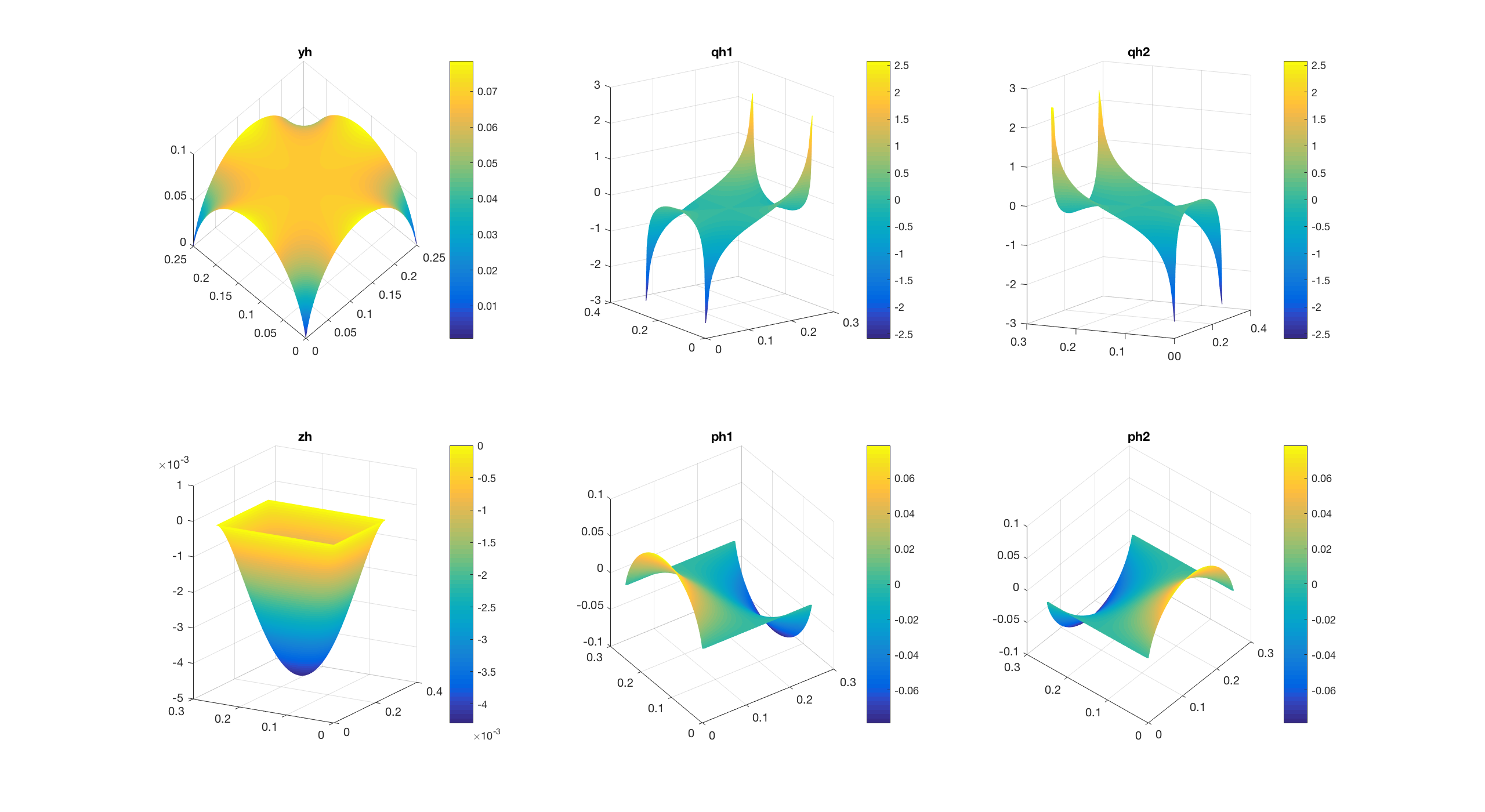
Figure 1: The primary state $y_{h}$, the primary flux $\bm{q}_{h}$, the dual state $z_{h}$, and the dual flux $\bm{p}_{h}$ for the 2D example

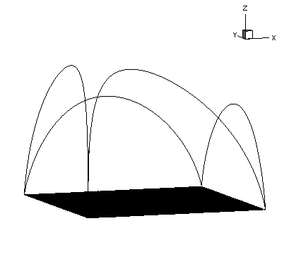
Figure 2: The optimal control $u_{h}$ for the 2D example

Next, we consider a 3D extension of the 2D example above. The domain is a cube $\Omega=[0,1/32]\times[0,1/32]\times[0,1/32]$, and the data is chosen as

$$f=0,\ \ y_{d}=(x^{2}+y^{2}+z^{2})^{s}\quad\mbox{and}\quad\gamma=1,$$

where $s=-1/4+10^{-5}$, so that $y_{d}\in H^{1}(\Omega)$. In this case, we did not attempt to determine the regularity of the control and other variables; we simply present the numerical results here.

As in the 2D example above, we do not have an explicit expression for the exact solution. Therefore, we solved the problem numerically for a triangulation with 196608 tetrahedrons, i.e., $h=2^{-12}\sqrt{3}$ and compared this reference solution against other solutions computed on meshes with larger $h$. The numerical results are shown in Table 2. The observed convergence rates for all variables are similar to the results for the 2D example above.

$h/\sqrt{3}$	$2^{-6}$	$2^{-7}$	$2^{-8}$	$2^{-9}$
$\left\lVert\bm{q}-\bm{q}_{h}\right\rVert_{0,\Omega}$	9.2640e-03	5.2580e-03	2.7462e-03	1.2475e-03
order	-	0.81712	0.93706	1.1384
$\left\lVert\bm{p}-\bm{p}_{h}\right\rVert_{0,\Omega}$	3.5425e-05	1.2283e-05	3.8463e-06	1.1022e-06
order	-	1.5281	1.6751	1.8032
$\left\lVert{y}-{y}_{h}\right\rVert_{0,\Omega}$	1.6040e-05	4.5070e-06	1.2191e-06	2.9781e-07
order	-	1.8314	1.8864	2.0333
$\left\lVert{z}-{z}_{h}\right\rVert_{0,\Omega}$	7.8545e-08	1.3058e-08	2.0042e-09	2.8775e-10
order	-	2.5886	2.7039	2.8001
$\left\lVert{u}-{u}_{h}\right\rVert_{0,\Gamma}$	4.5932e-04	1.8934e-04	7.1955e-05	2.4123e-05
order	-	1.2785	1.3958	1.5767

Table 2: Error of control $u$, state $y$, adjoint state $z$, and their fluxes $\bm{q}$ and $\bm{p}$.

6 Conclusions

We proposed an HDG method to approximate the solution of an optimal Dirichlet boundary control problems for the Poisson equation. We obtained a superlinear rate of convergence for the control in 2D under certain assumptions on the domain and the target state $y_{d}$. Numerical experiments confirmed our theoretical results.

Our results indicate HDG methods have potential for solving more complex Dirichlet boundary control problems. We plan to investigate HDG methods for Dirichlet boundary control of other PDEs, including convection dominated diffusion problems and fluid flows. These problems may involve solutions with large gradients or shocks, and it is natural to consider HDG methods for such problems.

Appendix A Local Solver

By simple algebraic operations in equation (35), we obtain the following formulas for the matrices $G_{1}$, $G_{2}$, $H_{1}$, and $H_{2}$ in (40):

$$G_{1} =B_{1}^{-1}B_{2}(B_{4}+B_{2}^{T}B_{1}^{-1}B_{2})^{-1}(B_{5}+B_{2}^{T}B_{1}^{-1}B_{3})-B_{1}^{-1}B_{3},$$

$$G_{2} =-(B_{4}+B_{2}^{T}B_{1}^{-1}B_{2})^{-1}(B_{5}+B_{2}^{T}B_{1}^{-1}B_{3}),$$

$$H_{1} =-B_{1}^{-1}B_{2}(B_{4}+B_{2}^{T}B_{1}^{-1}B_{2})^{-1},$$

$$H_{2} =(B_{4}+B_{2}^{T}B_{1}^{-1}B_{2})^{-1}.$$

In general, this process is impractical; however, for the HDG method described in this work, these matrices can be easily computed. This is one of the advantages of the HDG method. We briefly describe this process below.

Since the spaces $\bm{V}_{h}$ and $W_{h}$ consist of discontinuous polynomials, some of the system matrices are block diagonal and each block is small and symmetric positive definite. Let us call a matrix of this form a SSPD block diagonal matrix. The inverse of a SSPD block diagonal matrix is another SSPD block diagonal matrix, and the inverse can be easily constructed by computing the inverse of each small block. Furthermore, the inverse of each small block can be computed independently; and therefore computing the inverse can be easily done in parallel.

It can be checked that $B_{1}$ is a SSPD block diagonal matrix, and therefore $B_{1}^{-1}$ is easily computed and is also a SSPD block diagonal matrix. Therefore, the the matrices $G_{1}$, $G_{2}$, $H_{1}$, and $H_{2}$ are easily computed if $B_{4}+B_{2}^{T}B_{1}^{-1}B_{2}$ is also easily inverted. We show below that this is the case.

First, it can be checked that $B_{2}$ is block diagonal with small blocks, but the blocks are not symmetric or definite. This implies $B_{2}^{T}B_{1}^{-1}B_{2}$ is block diagonal with small nonnegative definite blocks. Next, $B_{4}=\begin{bmatrix}A_{5}&0\\ -A_{4}&A_{5}\end{bmatrix}$, where $A_{4}$ and $A_{5}$ are both SSPD block diagonal. Due to the structure of $B_{1}$ and $B_{2}$, the matrix $B_{2}^{T}B_{1}^{-1}B_{2}+B_{4}$ has the form $\begin{bmatrix}C_{1}&0\\ -A_{4}&C_{2}\end{bmatrix},$ where $C_{1}$ and $C_{2}$ are SSPD block diagonal. The inverse can be easily computed using the formula

$$\begin{bmatrix}C_{1}&0\\ -A_{4}&C_{2}\end{bmatrix}^{-1}=\begin{bmatrix}C_{1}^{-1}&0\\ C_{2}^{-1}A_{4}C_{1}^{-1}&C_{2}^{-1}\end{bmatrix}.$$

Furthermore, $C_{1}^{-1}$, $C_{2}^{-1}$ and $C_{2}^{-1}A_{4}C_{1}^{-1}$ are both SSPD block diagonal.

References

- [1] Thomas Apel, Mariano Mateos, Johannes Pfefferer, and Arnd Rösch. Error estimates for Dirichlet control problems in polygonal domains. http //arxiv.org/pdf/1704.08843v1.
- [2] N. Arada and J.-P. Raymond. Dirichlet boundary control of semilinear parabolic equations. I. Problems with no state constraints. Appl. Math. Optim., 45(2):125–143, 2002.
- [3] Faker Ben Belgacem, Henda El Fekih, and Hejer Metoui. Singular perturbation for the Dirichlet boundary control of elliptic problems. M2AN Math. Model. Numer. Anal., 37(5):883–850, 2003.
- [4] Eduardo Casas, Mariano Mateos, and Jean-Pierre Raymond. Penalization of Dirichlet optimal control problems. ESAIM Control Optim. Calc. Var., 15(4):782–809, 2009.
- [5] Eduardo Casas and Jean-Pierre Raymond. Error estimates for the numerical approximation of Dirichlet boundary control for semilinear elliptic equations. SIAM J. Control Optim., 45(5):1586–1611, 2006.
- [6] Aycil Cesmelioglu, Bernardo Cockburn, and Weifeng Qiu. Analysis of a hybridizable discontinuous Galerkin method for the steady-state incompressible Navier-Stokes equations. Math. Comp., 86(306):1643–1670, 2017.
- [7] Nagaiah Chamakuri, Christian Engwer, and Karl Kunisch. Boundary control of bidomain equations with state-dependent switching source functions in the ionic model. J. Comput. Phys., 273:227–242, 2014.
- [8] Lili Chang, Wei Gong, and Ningning Yan. Weak boundary penalization for Dirichlet boundary control problems governed by elliptic equations. J. Math. Anal. Appl., 453(1):529–557, 2017.
- [9] Yanlai Chen, Bernardo Cockburn, and Bo Dong. Superconvergent HDG methods for linear, stationary, third-order equations in one-space dimension. Math. Comp., 85(302):2715–2742, 2016.
- [10] Yanping Chen. Superconvergence of mixed finite element methods for optimal control problems. Math. Comp., 77(263):1269–1291, 2008.
- [11] Sudipto Chowdhury, Thirupathi Gudi, and A. K. Nandakumaran. Error bounds for a Dirichlet boundary control problem based on energy spaces. Math. Comp., 86(305):1103–1126, 2017.
- [12] Bernardo Cockburn, Jayadeep Gopalakrishnan, and Raytcho Lazarov. Unified hybridization of discontinuous Galerkin, mixed, and continuous Galerkin methods for second order elliptic problems. SIAM J. Numer. Anal., 47(2):1319–1365, 2009.
- [13] Bernardo Cockburn, Jayadeep Gopalakrishnan, Ngoc Cuong Nguyen, Jaume Peraire, and Francisco-Javier Sayas. Analysis of HDG methods for Stokes flow. Math. Comp., 80(274):723–760, 2011.
- [14] Bernardo Cockburn and Kassem Mustapha. A hybridizable discontinuous Galerkin method for fractional diffusion problems. Numer. Math., 130(2):293–314, 2015.
- [15] Bernardo Cockburn and Jiguang Shen. A hybridizable discontinuous Galerkin method for the -Laplacian. SIAM J. Sci. Comput., 38(1):A545–A566, 2016.
- [16] A. R. Danilin. Asymptotics of the solution of a problem of optimal boundary control of a flow through a part of the boundary. Tr. Inst. Mat. Mekh., 20(4):116–127, 2014.
- [17] J. C. de los Reyes and K. Kunisch. A semi-smooth Newton method for control constrained boundary optimal control of the Navier-Stokes equations. Nonlinear Anal., 62(7):1289–1316, 2005.
- [18] Klaus Deckelnick, Andreas Günther, and Michael Hinze. Finite element approximation of Dirichlet boundary control for elliptic PDEs on two- and three-dimensional curved domains. SIAM J. Control Optim., 48(4):2798–2819, 2009.
- [19] A. V. Fursikov, M. D. Gunzburger, and L. S. Hou. Boundary value problems and optimal boundary control for the Navier-Stokes system: the two-dimensional case. SIAM J. Control Optim., 36(3):852–894, 1998.
- [20] A. V. Fursikov, M. D. Gunzburger, and L. S. Hou. Optimal Dirichlet control and inhomogeneous boundary value problems for the unsteady Navier-Stokes equations. In Control and partial differential equations (Marseille-Luminy, 1997), volume 4 of ESAIM Proc., pages 97–116. Soc. Math. Appl. Indust., Paris, 1998.
- [21] A. V. Fursikov, M. D. Gunzburger, and L. S. Hou. Optimal boundary control for the evolutionary Navier-Stokes system: the three-dimensional case. SIAM J. Control Optim., 43(6):2191–2232, 2005.
- [22] Wei Gong and Ningning Yan. Mixed finite element method for Dirichlet boundary control problem governed by elliptic PDEs. SIAM J. Control Optim., 49(3):984–1014, 2011.
- [23] M. D. Gunzburger, L. S. Hou, and Th. P. Svobodny. Analysis and finite element approximation of optimal control problems for the stationary Navier-Stokes equations with Dirichlet controls. RAIRO Modél. Math. Anal. Numér., 25(6):711–748, 1991.
- [24] M. D. Gunzburger and S. Manservisi. The velocity tracking problem for Navier-Stokes flows with boundary control. SIAM J. Control Optim., 39(2):594–634, 2000.
- [25] Max D. Gunzburger, LiSheng Hou, and Thomas P. Svobodny. Boundary velocity control of incompressible flow with an application to viscous drag reduction. SIAM J. Control Optim., 30(1):167–181, 1992.
- [26] Max D. Gunzburger and R. A. Nicolaides. An algorithm for the boundary control of the wave equation. Appl. Math. Lett., 2(3):225–228, 1989.
- [27] Michael Hinze and Karl Kunisch. Second order methods for boundary control of the instationary Navier-Stokes system. ZAMM Z. Angew. Math. Mech., 84(3):171–187, 2004.
- [28] L. S. Hou and S. S. Ravindran. A penalized Neumann control approach for solving an optimal Dirichlet control problem for the Navier-Stokes equations. SIAM J. Control Optim., 36(5):1795–1814, 1998.
- [29] C. Lehrenfeld. Hybrid Discontinuous Galerkin Methods for Incompressible Flow Problems. Master’s thesis, RWTH Aachen, May 2010.
- [30] Binjie Li and Xiaoping Xie. Analysis of a family of HDG methods for second order elliptic problems. J. Comput. Appl. Math., 307:37–51, 2016.
- [31] Wenbin Liu, Danping Yang, Lei Yuan, and Chaoqun Ma. Finite element approximations of an optimal control problem with integral state constraint. SIAM J. Numer. Anal., 48(3):1163–1185, 2010.
- [32] Mariano Mateos and Ira Neitzel. Dirichlet control of elliptic state constrained problems. Comput. Optim. Appl., 63(3):825–853, 2016.
- [33] S. May, R. Rannacher, and B. Vexler. Error analysis for a finite element approximation of elliptic Dirichlet boundary control problems. SIAM J. Control Optim., 51(3):2585–2611, 2013.
- [34] C. Meyer and A. Rösch. Superconvergence properties of optimal control problems. SIAM J. Control Optim., 43(3):970–985, 2004.
- [35] Kassem Mustapha, Maher Nour, and Bernardo Cockburn. Convergence and superconvergence analyses of HDG methods for time fractional diffusion problems. Adv. Comput. Math., 42(2):377–393, 2016.
- [36] N. C. Nguyen, J. Peraire, and B. Cockburn. An implicit high-order hybridizable discontinuous Galerkin method for linear convection-diffusion equations. J. Comput. Phys., 228(9):3232–3254, 2009.
- [37] N. C. Nguyen, J. Peraire, and B. Cockburn. An implicit high-order hybridizable discontinuous Galerkin method for nonlinear convection-diffusion equations. J. Comput. Phys., 228(23):8841–8855, 2009.
- [38] N. C. Nguyen, J. Peraire, and B. Cockburn. A hybridizable discontinuous Galerkin method for Stokes flow. Comput. Methods Appl. Mech. Engrg., 199(9-12):582–597, 2010.
- [39] G. Of, T. X. Phan, and O. Steinbach. An energy space finite element approach for elliptic Dirichlet boundary control problems. Numer. Math., 129(4):723–748, 2015.
- [40] Weifeng Qiu and Ke Shi. An HDG method for convection diffusion equation. J. Sci. Comput., 66(1):346–357, 2016.
- [41] Sivaguru S Ravindran. Finite element approximation of Dirichlet control using boundary penalty method for unsteady Navier–Stokes equations. ESAIM: Mathematical Modelling and Numerical Analysis, 51(3):825–849, 2017.
- [42] Sivaguru S. Ravindran. Finite element approximation of Dirichlet control using boundary penalty method for unsteady Navier-Stokes equations. ESAIM Math. Model. Numer. Anal., 51(3):825–849, 2017.
- [43] Yulian Spasov and Karl Kunisch. Dynamical system based optimal control of incompressible fluids. Boundary control. Eur. J. Mech. B Fluids, 25(2):153–163, 2006.
- [44] M. Stanglmeier, N. C. Nguyen, J. Peraire, and B. Cockburn. An explicit hybridizable discontinuous Galerkin method for the acoustic wave equation. Comput. Methods Appl. Mech. Engrg., 300:748–769, 2016.
- [45] Ruxandra Stavre. A boundary control problem for the blood flow in venous insufficiency. The general case. Nonlinear Anal. Real World Appl., 29:98–116, 2016.
- [46] B. Vexler. Finite element approximation of elliptic Dirichlet optimal control problems. Numer. Funct. Anal. Optim., 28(7-8):957–973, 2007.