Sub-Riemannian cubics in SU(2)

Abstract

Sub-Riemannian cubics are a generalisation of Riemannian cubics to a sub-Riemannian manifold. Cubics are curves which minimise the integral of the norm of the covariant acceleration. Sub-Riemannian cubics are cubics which are restricted to move in a horizontal subspace of the tangent space. When the sub-Riemannian manifold is also a Lie group, sub-Riemannian cubics correspond to what we call a sub-Riemannian Lie quadratic in the Lie algebra. The present article studies sub-Riemannian Lie quadratics in the case of $\mathfrak{su}(2)$, focusing on the long term dynamics.

I Sub-Riemannian cubics

Let $G$ be a matrix Lie group with a positive-definite bi-invariant inner product $\langle,\rangle_{B}$ on the Lie algebra $\mathfrak{g}:=TG_{e}$. Choose a positive-definite self-adjoint operator $\mathcal{J}$ with respect to $\langle,\rangle_{B}$. Now define $\langle,\rangle_{\mathcal{J}}$, by $\langle X,Y\rangle_{\mathcal{J}}=\langle X,\mathcal{J}Y\rangle_{B}$. Given a basis $\hat{e}_{1},\dots\hat{e}_{n}$ for $\mathfrak{g}$, define an $n\times n$ matrix $\mathcal{J}_{ij}$ by $\mathcal{J}_{ij}=\langle\hat{e}_{i},\hat{e}_{j}\rangle_{\mathcal{J}}$. Then given $V=v_{k}\hat{e}_{k}\in\mathfrak{g},\,v_{k}\in\mathbb{R}$, we can compute $\mathcal{J}V=v_{i}\mathcal{J}_{ij}\hat{e}_{j}$, where repeated indicies are summed.

A left-invariant metric $\langle,\rangle$ is defined on $TG$ by the formula $\langle X,Y\rangle_{g}:=\langle g^{-1}X,g^{-1}Y\rangle_{\mathcal{J}}$. Then given a vector subspace of $\delta_{1}\subset\mathfrak{g}$, we define a left-invariant distribution on $G$ to be the vector sub-bundle $\delta$ of $TG$, whose fibre $\delta_{g}$ over $g$ is $g\delta_{1}$.

Previous work Camarinha et al. (2001); Pauley and Noakes (2012); GiambA et al. (2002); Noakes (2003); Noakes and Ratiu (2016); Noakes (2006a) has investigated the critical points of the functional

$$S\left[\widetilde{x}\right]:=\int_{0}^{T}\langle\nabla_{t}\dot{\widetilde{x}},\nabla_{t}\dot{\widetilde{x}}\rangle_{\hat{x}}\,dt,$$ (1)

where $\widetilde{x}:\left[0,T\right]\rightarrow M$, and $\widetilde{x}(0),\widetilde{x}(T),\dot{\widetilde{x}}(0)$ and $\dot{\widetilde{x}}(T)$ are given. $\nabla_{t}\dot{\widetilde{x}}$ denotes the covariant acceleration, and $M$ is a Riemannian manifold. In this situation critical points of $S$ are called Riemannian cubics. We now consider the case where, $M=G$ and $\dot{\widetilde{x}}$ is constrained to be in the distribution $\delta$. With this constraint, we will call critical points of $S$ a sub-Riemannian cubic.

Note that restricting the original Riemannian metric to the distribution makes $G$ a sub-Riemannian manifold Montgomery (2006). When the metric is not bi-invariant, $\mathcal{J}\neq I$, where $I$ is the identity matrix, we need an underlying Riemannian metric to define $\nabla_{t}\dot{\widetilde{x}}$, which is not necessarily restricted to the distribution.

The equations for normal sub-Riemannian cubics can be derived from the Pontryagin Maximum Principle (PMP). For a reference on the PMP see L. S. Pontryagin, V. G. Boltyanskii, R. V. Gamkrelidze, E. F. Mishechenko (1963). Usually the PMP applies for control systems on $\mathbb{R}^{n}$ but there is a version for control systems on a Lie group Sachkov (2009).

As $G$ is left-invariant $\dot{\widetilde{x}}$ is constrained by the equation

$$\dot{\widetilde{x}}:=\widetilde{x}\,\widetilde{V},$$ (2)

where $\widetilde{V}:\left[0,T\right]\rightarrow\delta_{1}$. We also require $\delta_{1}$ to be a bracket generating subset of $\mathfrak{g}$.

Let left Lie reduction by $\widetilde{x}$ be denoted $L^{-1}$. Then the left Lie reduction of the covariant acceleration $\nabla_{t}\dot{\widetilde{x}}$ to $\mathfrak{g}$ includes a first order derivative of $\widetilde{V}$,

$$L^{-1}(\nabla_{t}\dot{\widetilde{x}})=\dot{\widetilde{V}}-\mathcal{J}^{-1}\left[\mathcal{J}\widetilde{V},\widetilde{V}\right].$$ (3)

To use the PMP define a new control function $u:\left[0,T\right]\rightarrow\mathfrak{g}$, and treat $\widetilde{V}$ as an additional state variable. So to minimise $S[\widetilde{x}]$ subject to the constraints

$$\dot{\widetilde{x}} =\widetilde{x}\,\widetilde{V},$$ (4)

$$\dot{\widetilde{V}} =u,$$ (5)

we form the PMP Hamiltonian, $H$, given by

$$H(\widetilde{x},\widetilde{V},u,\lambda,\vartheta,\nu):=\lambda(\widetilde{x}\,\widetilde{V})+\vartheta(u)+\frac{\nu}{2}\left\|u-\mathcal{J}^{-1}\left[\mathcal{J}\widetilde{V},\widetilde{V}\right]\right\|^{2}_{\mathcal{J}},$$ (6)

where $\lambda\in T^{*}G_{\widetilde{x}}$ and $\vartheta\in\mathfrak{g}^{*}$ are the co-states, and $\nu\leq 0$. Then the PMP says maximising $H$ for all $t$ is a necessary condition for minimising $S$.

By the PMP, the co-states are required to satisfy

$$\dot{\lambda}(y) =-dH_{\widetilde{x}}(y)=-\lambda(y\widetilde{V}),$$

$$\dot{\vartheta}(Z) =-dH_{\widetilde{V}}(Z)=-\lambda(\widetilde{x}Z)-\nu\left\langle-\mathcal{J}^{-1}\left[\mathcal{J}Z,\widetilde{V}\right]+\mathcal{J}^{-1}\left[\mathcal{J}\widetilde{V},Z\right],u-\mathcal{J}^{-1}\left[\mathcal{J}\widetilde{V},\widetilde{V}\right]\right\rangle_{\mathcal{J}}$$

$\forall y\in TG_{\widetilde{x}}$ and $Z\in\mathfrak{g}$. $\lambda\in T^{*}G_{\widetilde{x}}$ can be associated with a $\lambda^{*}\in\mathfrak{g}^{*}$ via left multiplication, $\Lambda^{*}(V)=\lambda(L(\widetilde{x})V)$. Differentiating $\Lambda^{*}$,

$$\dot{\Lambda^{*}}(y) =\dot{\lambda}(\widetilde{x}\,y)+\lambda(\dot{\widetilde{x}}\,y)$$

$$=-\lambda(\widetilde{x}\,y\,\widetilde{V})+\lambda(\widetilde{x}\,\widetilde{V}y)$$

$$=-\Lambda^{*}(y\,\widetilde{V})+\Lambda^{*}(\widetilde{V}y)$$

$$=\Lambda^{*}\left(\left[\widetilde{V},y\right]\right).$$

Finally $\Lambda^{*}$ can be associated with $\Lambda\in\mathfrak{g}$ via the bi-invariant inner product, $\langle,\rangle_{B}$

$$\Lambda^{*}(y)=\langle\Lambda,y\rangle_{B}.$$

Likewise for $\vartheta$ there is an associated $\Theta\in\mathfrak{g}$.

$$\vartheta(w)=\langle\Theta,w\rangle_{B}.$$

This gives the following equations for the costates

$$\dot{\Lambda} =\left[\Lambda,\widetilde{V}\right],$$

$$\dot{\Theta} =-\Lambda-\nu\bigg{(}\mathcal{J}\left[\widetilde{V},u\right]-\left[\mathcal{J}\widetilde{V},u\right]$$

$$+\mathcal{J}\left[\widetilde{V},\mathcal{J}^{-1}\left[\mathcal{J}\widetilde{V},\widetilde{V}\right]\right]-\left[\mathcal{J}\widetilde{V},\mathcal{J}^{-1}\left[\mathcal{J}\widetilde{V},\widetilde{V}\right]\right]\bigg{)}.$$

By the PMP there are two cases to consider.

I.0.1 Normal case

In the normal case, $\nu<0$, the optimal control $u^{*}$ must maximise $H$. From now on we consider the case when $\langle,\rangle_{\mathcal{J}}$ is simply bi-invariant and so $\mathcal{J}=I$. We now use the notation $\langle,\rangle:=\langle,\rangle_{\mathcal{J}}=\langle,\rangle_{B}$. Without loss of generality set $\nu=-1$. Hence in the normal case, the PMP Hamiltonian can equivalently written as

$$H=\big{\langle}\Lambda,\widetilde{V}\big{\rangle}+\big{\langle}\Theta,u\big{\rangle}-\frac{1}{2}\big{\langle}u,u\big{\rangle}.$$

Maxima occur when $dH(u^{*})_{u}=0$, so

$$\big{\langle}\Theta,u^{*}\big{\rangle}-\big{\langle}u,u^{*}\big{\rangle}=0.$$ (7)

Therefore optimal controls occur when $\mathrm{proj}_{\delta_{1}}(\Theta)=u=\dot{\widetilde{V}}$. The equations for the costates reduce to a single equation, which gives the following theorem.

Theorem I.1.

$\widetilde{x}$ is a normal sub-Riemannian cubic if and only if

$$\ddot{\Theta}=\left[\dot{\Theta},\widetilde{V}\right].$$ (8)

Remark.

Denote the projection of $\Theta$ onto the orthogonal complement, $\perp$, of $\delta_{1}$ by $\varphi=\mathrm{proj}_{\perp}(\Theta)$. Let $\delta_{1}=\mathfrak{g}$. Then the resulting equations for normal sub-Riemannian cubics match the bi-invariant Riemannian case, $\dddot{\widetilde{V}}=\left[\ddot{\widetilde{V}},\widetilde{V}\right]$ Noakes and Ratiu (2016). In general solutions to (8) are hard to find.

Remark.

One subclass of solutions are the so called linear Lie quadratics. In this case, $\varphi=\varphi_{0}$ and $\widetilde{V}=(q_{0}+q_{1}t+q_{2}t^{2})\widetilde{V}_{0}$, where $q_{0},q_{1},q_{2}\in\mathbb{R}$, $\widetilde{V}_{0}$ is a constant in $\delta_{1}$, and $\varphi_{0}$ is a constant in the orthogonal complement of $\delta_{1}$.

$\dot{\Theta}$ can be found in terms of $\widetilde{x}$. Rewrite (8), take the adjoint and integrate,

$$\mathrm{Ad}(\widetilde{x})\left(\ddot{\Theta}+[\widetilde{V},\dot{\Theta}]\right)=0$$

$$\implies\dot{\Theta}=\mathrm{Ad}(\widetilde{x}^{-1})\mathcal{A}$$

where $\mathcal{A}\in\mathfrak{g}$. This simply reflects the fact that $\dot{\Theta}$ satisfies a Lax equation Noakes (2006b) and is therefore isospectral.

I.0.2 Abnormal case

The abnormal case is given by $\nu=0$. As before, the PMP Hamiltonian can be written as

$$H=\big{\langle}\Lambda,\widetilde{V}\big{\rangle}+\big{\langle}\Theta,u\big{\rangle}.$$

Maxima occur when $dH(u^{*})_{u}=0$. Immediately this requires $\mathrm{proj}_{\delta_{1}}(\Theta)=0$, so there is no way to determine $u$ from the PMP.

I.0.3 Bounds

Given some function $f$, we say that $f$ is $\mathcal{O}(t^{n})$, when for some $c>0$, $\left|f\right|\leq c\left|t^{n}\right|$, for all $t\in\mathbb{R}$.

Corollary I.1.

$$\big{\langle}\ddot{\widetilde{V}},\widetilde{V}\big{\rangle}-\frac{1}{2}\big{\langle}\dot{\widetilde{V}},\dot{\widetilde{V}}\big{\rangle} =c_{1},$$ (9)

$$\big{\langle}\ddot{\widetilde{V}},\ddot{\widetilde{V}}\big{\rangle}+\big{\langle}\dot{\varphi},\dot{\varphi}\big{\rangle} =c_{2},$$ (10)

where $c_{1}\in\mathbb{R}$ and $c_{2}\geq 0$.

Proof.

First take the inner product of (8) and $\widetilde{V}$ to find $\langle\dddot{\widetilde{V}},\widetilde{V}\rangle=0$. Next take the inner product of (8) with $\ddot{\widetilde{V}}+\dot{\varphi}$ to find $\langle\dddot{\widetilde{V}},\ddot{\widetilde{V}}\rangle+\langle\dot{\varphi},\dot{\varphi}\rangle=0$. Integrating these gives the result. ∎

Corollary I.2.

$$\frac{1}{2}c_{1}t^{2}+c_{5}t+c_{6}\leq\big{\langle}\widetilde{V},\widetilde{V}\big{\rangle}\leq\mathcal{O}(t^{4}).$$

Proof.

As $\big{\langle}\dot{\varphi},\dot{\varphi}\big{\rangle}\geq 0$, we have $\big{\langle}\ddot{\widetilde{V}},\ddot{\widetilde{V}}\big{\rangle}\leq c_{2}$. This argument can be repeated for the components of $\ddot{\widetilde{V}}$, so given $\widetilde{V}=v_{k}(t)\widehat{e}_{k}$, then $\ddot{v}_{k}^{2}\big{\langle}\hat{e}_{k},\hat{e}_{k}\big{\rangle}\leq c_{2}$. As we are working with the bi-invariant metric, we have $-\sqrt{c_{2}}\leq\ddot{v_{k}}\leq\sqrt{c_{2}}$ and so $|v_{k}|\leq\frac{1}{2}\sqrt{c_{2}}t^{2}+c_{3}t+c_{4}$, where $c_{3}$ and $c_{4}$ are some other constants. Therefore $\big{\langle}\widetilde{V},\widetilde{V}\big{\rangle}$ is bounded above by $\mathcal{O}(t^{4})$.

The same argument can be used to to show $\big{\langle}\dot{\varphi},\dot{\varphi}\big{\rangle}$ is bounded above a constant, and then $\left\|\varphi\right\|$ is bounded above by a linear function. This then shows $\big{\langle}\varphi,\varphi\big{\rangle}$ is bounded above by $\mathcal{O}(t^{2})$.

Equation (9) can be written as

$$\frac{d^{2}}{dt^{2}}\left(\big{\langle}\widetilde{V},\widetilde{V}\big{\rangle}\right)=c_{1}+\frac{3}{2}\big{\langle}\dot{\widetilde{V}},\dot{\widetilde{V}}\big{\rangle}.$$ (11)

Immediately this yields the lower bound $\big{\langle}\widetilde{V},\widetilde{V}\big{\rangle}\geq\frac{1}{2}c_{1}t^{2}+c_{5}t+c_{6}$ where $c_{5}$ and $c_{6}$ are other constants. ∎

II Sub-Riemannian Lie quadratics and symmetric pairs

II.1 Symmetric pairs

Let $(\mathfrak{g},\mathfrak{h})$ be a symmetric pair, namely $\mathfrak{g}=\mathfrak{m}+\mathfrak{h}$ where the following properties hold

$$\left[\mathfrak{m},\mathfrak{m}\right] \subseteq\mathfrak{h},$$

$$\left[\mathfrak{h},\mathfrak{m}\right] \subseteq\mathfrak{m},$$

$$\left[\mathfrak{h},\mathfrak{h}\right] \subseteq\mathfrak{m}.$$

An example is $\mathfrak{su}(2)$ where $\mathfrak{m}$ is spanned by the Pauli matrices $i\sigma_{1}$ and $i\sigma_{2}$, and $\mathfrak{h}$ is spanned by $i\sigma_{3}$. Suppose we set $\delta_{1}=\mathfrak{m}$. The equations for normal sub-Riemannian cubics in $\mathfrak{g}$ separate into two components.

$$\ddot{\varphi} =\left[\ddot{\widetilde{V}},\widetilde{V}\right],$$

$$\dddot{\widetilde{V}} =\left[\dot{\varphi},\widetilde{V}\right].$$

Integrating the first equation and substituting leaves

$$\dddot{\widetilde{V}} =\left[\left[\dot{\widetilde{V}},\widetilde{V}\right],\widetilde{V}\right]+\left[\widetilde{\mathcal{C}},\widetilde{V}\right].$$ (12)

We call $\widetilde{V}$ which satisfy this equation a sub-Riemannian Lie quadratic. One simple solution to this is $\widetilde{V}=\widetilde{V}_{0}+\widetilde{V}_{1}t$, where $\widetilde{V}_{0}$ and $\widetilde{V}_{1}$ are chosen so $\left[\widetilde{V}_{0},\widetilde{V}_{1}\right]=\widetilde{C}$. We call sub-Riemannian Lie quadratics null when $\widetilde{\mathcal{C}}=0$.

II.2 Duality

We say $\widetilde{W}$ is dual to $\widetilde{V}$, when

$$\widetilde{W} =-\mathrm{Ad}(\widetilde{x})\widetilde{V},$$ (13)

$$\dot{\widetilde{y}} =\widetilde{y}\,\widetilde{W},$$ (14)

where $\widetilde{y}=\widetilde{x}^{-1}$.

In the null case, $\widetilde{\mathcal{C}}=0$, $\widetilde{V}$ is dual to a non-null Riemannian Lie quadratic, $V$, which is defined by the equation

$$\ddot{V}=[\dot{V},V]+C.$$

Duality was considered for Riemannian Lie quadratics in Noakes (2006a). We investigate the sub-Riemannian case.

Theorem II.1.

$\widetilde{V}$ is dual to a rescaled non-null Riemannian Lie quadratic.

Proof.

Recall that for any other function $Z$

$$\frac{d}{dt}\left(\mathrm{Ad}\left(\widetilde{x}\right)Z\right)=\mathrm{Ad}(\widetilde{x})\left(\dot{Z}+\left[\widetilde{V},Z\right]\right).$$ (15)

Computing derivatives,

$$\dot{\widetilde{W}} =-\mathrm{Ad}(\widetilde{x})\left(\dot{\widetilde{V}}\right),$$

$$\ddot{\widetilde{W}} =-\mathrm{Ad}(\widetilde{x})\left(\ddot{\widetilde{V}}+\left[\widetilde{V},\dot{\widetilde{V}}\right]\right),$$

$$\dddot{\widetilde{W}} =-\mathrm{Ad}(\widetilde{x})\left(\dddot{\widetilde{V}}+\left[\widetilde{V},\ddot{\widetilde{V}}\right]+\left[\widetilde{V},\ddot{\widetilde{V}}+\left[\widetilde{V},\dot{\widetilde{V}}\right]\right]\right),$$

which gives

$$\dddot{\widetilde{W}} =-2\mathrm{Ad}(\widetilde{x})\left(\left[\widetilde{V},\ddot{\widetilde{V}}\right]+\left[\widetilde{V},\left[\widetilde{V},\dot{\widetilde{V}}\right]\right]\right).$$

Then

$$\left[\widetilde{W},\ddot{\widetilde{W}}\right]=\mathrm{Ad}(\widetilde{x})\left(\left[\widetilde{V},\ddot{\widetilde{V}}\right]+\left[\widetilde{V},\left[\widetilde{V},\dot{\widetilde{V}}\right]\right]\right),$$

and so

$$\dddot{\widetilde{W}}=2\left[\ddot{\widetilde{W}},\widetilde{W}\right].$$

Integrating this equation leaves a reparameterised non-null Riemannian Lie quadratic

$$\ddot{\widetilde{W}}=2\left[\dot{\widetilde{W}},\widetilde{W}\right]+\widetilde{\mathcal{D}}.$$ (16)

Without loss of generality, let $\widetilde{x}(0)=I$. Consider the equations for $\widetilde{W}$ and $\widetilde{V}$ at $t=0$. Clearly $\widetilde{V}(0)=\widetilde{W}(0)$, $\dot{\widetilde{V}}(0)=\dot{\widetilde{W}}(0)$, and $\ddot{\widetilde{W}}(0)=\ddot{\widetilde{V}}(0)+\left[\widetilde{V}(0),\dot{\widetilde{V}}(0)\right]$. First this shows $\widetilde{W}$ is no longer constrained to $\delta_{1}$. Additionally we must have $\widetilde{\mathcal{D}}=\ddot{\widetilde{V}}(0)+3\left[\widetilde{V}(0),\dot{\widetilde{V}}(0)\right]$.

Now let $V(t)=a\widetilde{W}(b\,t)$, where $a,b\in\mathbb{R}$. Setting $a=2b$, and $\mathcal{C}=2b^{3}\widetilde{\mathcal{D}}$, $V$ satisfies

$$\ddot{V}=\left[\dot{V},V\right]+\mathcal{C},$$ (17)

which is the equation for a non null Riemannian Lie quadratic. ∎

Note if we define $x:[0,T]\rightarrow G$, and $\dot{x}=xV$, then there is no clear relation between $x$, a non-null Riemannian cubic and $\widetilde{x}$. If $\mathcal{C}=0$ then the Lie quadratic is called null Noakes (2003). It is possible to integrate the equation for $V$ in certain groups. This can occur in a non-trivial way if $\ddot{\widetilde{V}}(0)=0$ and $\dot{\widetilde{V}}(0)=0$ or $\widetilde{V}(0)=0$. Let

$$W=-\mathrm{Ad}(x)V.$$

Computing derivatives, we find

$$\ddot{W}=0,$$

which gives $W=W_{0}+W_{1}t$, where the $W_{k}$ are constant matrices. If $V$ was known it would be possible to work backwards and compute $\widetilde{x}$ using the work of Noakes (2006b).

II.3 SU(2)

Let $G=\mathrm{SU}(2)$. Take $\delta_{1}=\mathrm{span}\left(\{\hat{e}_{1},\hat{e}_{2}\}\right)=\mathrm{span}\left(\frac{i}{\sqrt{2}}\{\sigma_{1},\sigma_{2}\}\right)$, where $\sigma_{i}$ are the Pauli matrices. Let $\widetilde{\mathcal{C}}=C\frac{i}{\sqrt{2}}\sigma_{3}$, where $C\in\mathbb{R}$. Recall $\mathfrak{su}(2)$ can be identified with $\mathfrak{so}(3)$. $\mathfrak{so}(3)$ can then be identified with Euclidean three space, $\mathbb{E}^{3}$, with the cross product. As a consquence of the vector triple product formula, we can write for $\widetilde{V}$ in $\mathfrak{su}(2)$

$$\dddot{\widetilde{V}}=2\left(\left\langle\widetilde{V},\dot{\widetilde{V}}\right\rangle\widetilde{V}-\left\langle\widetilde{V},\widetilde{V}\right\rangle\dot{\widetilde{V}}\right)+[\widetilde{\mathcal{C}},\widetilde{V}].$$ (18)

We can identify $\widetilde{V}=v_{1}(t)\hat{e}_{1}+v_{2}(t)\hat{e}_{2}$ with a $v\in\mathbb{C}$ by taking $v:=v_{1}+iv_{2}$. Then the sub-Riemannian cubic equation in $\delta_{1}$ can be written as

$$\dddot{v}=\frac{1}{2}v\left(\dot{\bar{v}}v-\dot{v}\bar{v}\right)-iCv.$$

Assuming $v(t)\neq 0$ for all t, define $\omega:\mathbb{R}\rightarrow\mathbb{S}^{1}\subset\mathbb{E}^{2}\cong\mathbb{C}$ by

$$\omega(t):=\frac{v(t)}{\|v(t)\|}.$$

Define $\mathrm{exp}(y)=(\cos(y),\sin(y))\equiv e^{iy}\in\mathbb{C}$. Choose a $\vartheta(t_{0})\in[0,2\pi)$ so that $\mathrm{exp}(\vartheta(t_{0}))=\omega(t_{0})$. Then there is a unique continuous function $\vartheta:\mathbb{R}\rightarrow\mathbb{R}$ such that the diagram

commutes. Then we have $v(t)=q(t)(\cos(\vartheta(t)),\sin(\vartheta(t)))=qe^{i\vartheta}$, where $q(t)=\|v(t)\|=\|\widetilde{V}\|$.

Substituting back, and taking the real and imaginary components gives the two equations

$$\dddot{q}-3\dot{q}\,\dot{\vartheta}^{2}-3q\,\ddot{\vartheta}\dot{\vartheta} =0,$$ (19)

$$q\dddot{\vartheta}+3\dot{q}\,\ddot{\vartheta}+3\ddot{q}\,\dot{\vartheta}-q\,\dot{\vartheta}^{3}+q^{3}\,\dot{\vartheta}+C\,q =0.$$ (20)

Multiplying the first equation by $r$, and integrating leaves

$$-\frac{1}{2}\dot{q}^{2}+\ddot{q}q-\frac{3}{2}q^{2}\dot{\vartheta}^{2}+c_{1}=0,$$

where $c_{1}\in\mathbb{R}$. Note that equation follows directly from equation (11), but we use the complex structure to show several additional properties.

II.4 $c_{1}>0$

Let $c_{1}>0$. Recall $\langle V,V\rangle$ is at most $\mathcal{O}(t^{4})$. Therefore $q$ increases no faster than $\mathcal{O}(t^{2})$. Likewise $\dot{q}^{2}+q^{2}\dot{\vartheta}^{2}$ must not increase faster than $\mathcal{O}(t^{2})$.

Also note $q^{2}\dot{\vartheta}^{2}\leq c_{2}+c_{1}$. Recall $q^{2}$ was bounded below by a quadratic and above by $\mathcal{O}(t^{4})$, so at most $\dot{\vartheta}^{2}=\mathcal{O}(t^{-2})$. Additionally $q^{2}\dot{\vartheta}^{2}$ is at most $\mathcal{O}(t^{-2})$. Therefore,

$$\frac{-1}{2}\dot{q}^{2}+\ddot{q}q=c_{1}+\mathcal{O}(t^{-2}).$$

First set $Y=\dot{q}^{2}$. Then it follows

$$-Y+\frac{dY}{dq}q=2c_{1}+\mathcal{O}(t^{-2}),$$

so

$$\frac{d}{dq}\left(\frac{Y}{q}\right)=\frac{2c_{1}+\mathcal{O}(t^{-2})}{q^{2}}.$$

Integrating with respect to $q$

$$\dot{q}^{2}=c_{7}q-2c_{1}+\mathcal{O}(t^{-2}),$$

where $c_{7}\geq 0$. Up to $\mathcal{O}(t^{-2})$ error, and as $q$ is at most $\mathcal{O}(t^{2})$, we can write

$$\dot{q}=\left(c_{7}q-2c_{1}\right)^{\frac{1}{2}}+\left(c_{7}q-2c_{1}\right)^{-\frac{1}{2}}\mathcal{O}(t^{-2}).$$

Then

$$\frac{\dot{q}}{c_{7}q-2c_{1}}=1+\mathcal{O}(t^{-2}).$$

Integrating with respect to $t$

$$\frac{2(c_{7}q-2c_{1})^{\frac{1}{2}}}{c_{7}}=t+\frac{c_{8}}{c_{7}}+\mathcal{O}(t^{-1}),$$

which gives

$$q=\frac{(c_{7}t+c_{8})^{2}}{4c_{7}}+\frac{2c_{1}}{c_{7}}+\mathcal{O}(t^{-1}).$$

III Asymptotics

In $G=\mathrm{SU}(2)$, and with $c_{1}>0$, it is possible to show that long term asymptotes exist. For Riemannian cubics in $\mathrm{SO}(3)$, it was established that a limit exists in Noakes (2003). In $\mathrm{SU}(2)$, we can show that the limit

$$\alpha_{\pm}(\widetilde{V})=\lim_{t\rightarrow\pm\infty}\frac{\widetilde{V}}{\left\|\widetilde{V}\right\|},$$

exists. Using the (smooth) identification of $\delta_{1}$ with $\mathbb{C}$, we can equivalently show $\vartheta$ tends to a constant

$$\alpha_{\pm}=\lim_{t\rightarrow\pm\infty}\vartheta,$$

recalling the definition of $\vartheta$ from the previos section.

Theorem III.1.

$\alpha_{\pm}(\widetilde{V})=\lim_{t\rightarrow\pm\infty}\widetilde{V}/\left\|\widetilde{V}\right\|$ exists.

Proof.

Note that we only need to consider $t\rightarrow\infty$, as $\widetilde{V}$ can be re-parameterised. Using results from section (II.4), $\dot{\vartheta}$ behaves at most like $\mathcal{O}(t^{-2})$,

$$|\dot{\vartheta}|\leq\frac{1}{d_{1}t^{2}},$$

as $q$ is bounded by a quadratic. First note that for $s\geq r$

$$\left|\vartheta(s)-\vartheta(r)\right| \leq\int^{s}_{r}|\dot{\vartheta}|\,dt$$

$$\leq\frac{1}{d_{1}}\left(\frac{1}{r}-\frac{1}{s}\right).$$

We can show that for an unbounded sequence of increasing times, $t_{1},t_{2},\dots$, the sequence $\vartheta(t_{1}),\vartheta(t_{2}),\dots$ converges to a limit,

$$L=\lim_{n\rightarrow\infty}\vartheta(t_{n}).$$

Given some $\varepsilon\geq 0$, there exists a $N$ such that for all $n,m\geq N$, where $n\geq m$, we have

$$\left|\vartheta(t_{n})-\vartheta(t_{m})\right| \leq\frac{1}{d_{1}}\left(\frac{1}{t_{m}}-\frac{1}{t_{n}}\right)$$

$$\leq\frac{1}{d_{1}}\left(\frac{1}{t_{m}}\right)$$

$$\leq\frac{\varepsilon}{2}.$$

by choosing $t_{N}\geq(1+\frac{2}{d_{1}\varepsilon})$ and so the sequence is Cauchy. As $\vartheta$ is a real function, by completeness of $\mathbb{R}$, the sequence converges. So given $\varepsilon>0$, there exists an $N$ such that for all $n>N$

$$\left|L-\vartheta(t_{n})\right|\leq\frac{\varepsilon}{2}.$$

Using a similar argument as before, given an $\varepsilon\geq 0$, there exists a $T$ such that for $s,t\geq T$,

$$\left|\vartheta(s)-\vartheta(t)\right|\leq\frac{\varepsilon}{2}$$

Now choose $T=t_{N}$ and for $t\geq T$ we have

$$\left|L-\vartheta(T)\right|\leq\frac{\varepsilon}{2},$$

and

$$\left|\vartheta(T)-\vartheta(t)\right|\leq\frac{\varepsilon}{2}.$$

By the triangle inequality this gives

$$\left|L-\vartheta(t)\right|\leq\varepsilon.$$

Therefore

$$L=\lim_{t\rightarrow\infty}\vartheta.$$

Hence take $\alpha_{+}=L$. Likewise $\alpha_{-}$ exists by reparameterising. ∎

Using the identification this shows $\alpha_{\pm}(\widetilde{V})$ exists.

For null Riemannian cubics a similar limit was found in Theorem (5) of Noakes (2008). A similar approach can be used to establish a more precise statement on the convergence when the sub-Riemannian cubic is null. Define

$$\mathcal{V}=\widetilde{V}+\frac{1}{2\left\|\widetilde{V}\right\|^{2}}\ddot{\widetilde{V}}.$$ (21)

Recall $q(t)=\left\|\widetilde{V}(t)\right\|$.

Theorem III.2.

If $\widetilde{\mathcal{C}}=0$, $\left\|\frac{\mathcal{V}}{q}-\alpha_{\pm}(\widetilde{V})\right\|\leq\frac{\sqrt{c_{2}}}{2q^{3}}$.

Proof.

Again, considering $t\rightarrow\infty$ as the negative case can be found via re-parameterisation.

$$\frac{d}{dt}\left(\frac{\mathcal{V}}{q}\right) =\frac{\dot{\mathcal{V}}}{q}-\frac{\dot{q}\mathcal{V}}{q^{2}}$$

$$=\frac{1}{q}\left(\dot{\widetilde{V}}-\frac{\dot{q}}{q^{3}}\ddot{\widetilde{V}}+\frac{1}{2q^{2}}\left(2\left(\dot{q}q\widetilde{V}-q^{2}\dot{\widetilde{V}}\right)+[\widetilde{\mathcal{C}},\widetilde{V}]\right)\right)-\frac{\dot{q}}{q^{2}}\left(\widetilde{V}+\frac{1}{2q^{2}}\ddot{\widetilde{V}}\right)$$

$$=-\frac{3\dot{q}\ddot{\widetilde{V}}}{2q^{4}}+\frac{[\widetilde{\mathcal{C}},\widetilde{V}]}{2q^{3}}.$$

Then if $\widetilde{\mathcal{C}}=0$, and noting that $q>0$ , and for large enough $t$, $\dot{q}>0$, assuming $c_{7}>0$ and $c_{1}>0$,

$$\left\|\frac{\mathcal{V}(s)}{q(s)}-\frac{\mathcal{V}(r)}{q(r)}\right\| \leq\left\|\int^{s}_{r}\frac{d}{dt}\left(\frac{\mathcal{V}(t)}{q(t)}\right)\,dt\right\|$$

$$\leq\int_{r}^{s}\frac{3\dot{q}\sqrt{c_{2}}}{2q^{4}}\,dt$$

$$\leq\frac{\sqrt{c_{2}}}{2q(r)^{3}}-\frac{\sqrt{c_{2}}}{2q(s)^{3}}$$

$$\leq\frac{\sqrt{c_{2}}}{2q(r)^{3}}.$$

As $\ddot{\widetilde{V}}$ is bounded,

$$\lim_{t\rightarrow\infty}\frac{\mathcal{V}}{q}=\lim_{t\rightarrow\infty}\frac{\widetilde{V}}{q}=\alpha_{+}(\widetilde{V}).$$

So finally, taking the limit as $s\rightarrow\infty$

$$\left\|\alpha_{+}(\widetilde{V})-\frac{\mathcal{V}(r)}{q(r)}\right\|\leq\frac{\sqrt{c_{2}}}{2q(r)^{3}}.$$ (22)

∎

Corollary III.1.

$$\left\|q\,\alpha_{\pm}(\widetilde{V})-\widetilde{V}\right\|\leq\frac{\sqrt{c_{2}}}{2q^{2}}.$$ (23)

Proof.

Multiply equation (22) through by $q$. ∎

Recall from section (II.4), in the long term limit, assuming $c_{1},c_{7}>0$, $q$ approaches a quadratic. Hence in the long term $\widetilde{V}=q\,\alpha_{+}(\widetilde{V})+\mathcal{O}(t^{-4})$

In the non-null case, a different estimate can be made for $\widetilde{V}$.

$$\frac{\mathcal{V}(s)}{q(s)}-\frac{\mathcal{V}(r)}{q(r)}-\int_{r}^{s}\frac{[\widetilde{\mathcal{C}},\widetilde{V}]}{2q^{3}}\,dt =-\int_{r}^{s}\frac{3\dot{q}\ddot{\widetilde{V}}}{2q^{4}}\,dt.$$

As before, taking norms, and letting $s\rightarrow\infty$,

$$\left\|\alpha_{+}(\widetilde{V})-\frac{\mathcal{V}(r)}{q(r)}-\int_{r}^{\infty}\frac{[\widetilde{\mathcal{C}},\widetilde{V}]}{2q^{3}}dt\right\| \leq\frac{\sqrt{c_{2}}}{2q(r)^{3}}.$$

Multiplying through by $q$, we can deduce

$$\widetilde{V}(r)=q(r)\alpha_{+}(\widetilde{V})-q(r)\left[\widetilde{\mathcal{C}},\int_{r}^{\infty}\frac{\widetilde{V}}{2q^{3}}\,dt\right]+\mathcal{O}(r^{-4}).$$ (24)

With this we can estimate $V(r)$ recursively up to $\mathcal{O}(r^{-4})$ error.

Theorem III.3.

$$\widetilde{V}(r)=q(r)\alpha_{+}(\widetilde{V})-q(r)\int_{r}^{\infty}\frac{1}{2q(t)^{2}}\,dt\,\left[\widetilde{\mathcal{C}},\alpha_{+}(\widetilde{V})\right]+\mathcal{O}(r^{-4}).$$

Proof.

By equation (24), substituting $\widetilde{V}(r)$ back

$$\widetilde{V}(r) =q(r)\alpha_{+}(\widetilde{V})-q(r)\int_{r}^{\infty}\frac{1}{2q(t)^{2}}\,dt\,\left[\widetilde{\mathcal{C}},\alpha_{+}(\widetilde{V})\right]$$

$$+q(r)\int_{r}^{\infty}\frac{[\widetilde{\mathcal{C}},\mathcal{O}(t^{-4})]}{2q(t)^{2}}dt+q(r)\int_{r}^{\infty}\frac{\left[\widetilde{\mathcal{C}},\ \left[\widetilde{\mathcal{C}},\int_{t}^{\infty}\frac{\widetilde{V}(s)}{2q(s)^{3}}\,ds\right]\right]}{2q(t)^{2}}dt+\mathcal{O}(r^{-4}).$$

We should ignore terms smaller than $\mathcal{O}(t^{-4})$. Also recall $\widetilde{V}$ behaves like $\mathcal{O}(t^{2})$ for large $t$.

$$\widetilde{V}(r) =q(r)\alpha_{+}(\widetilde{V})-q(r)\int_{r}^{\infty}\frac{1}{2q(t)^{2}}\,dt\,\left[\widetilde{\mathcal{C}},\alpha_{+}(\widetilde{V})\right]$$

$$+q(r)\int_{r}^{\infty}\frac{[\widetilde{\mathcal{C}},\mathcal{O}(t^{-4})]}{2q(t)^{3}}dt+q(r)\int_{r}^{\infty}\frac{\left[\widetilde{\mathcal{C}},\ \left[\widetilde{\mathcal{C}},\mathcal{O}(t^{-3})\right]\right]}{2q(t)^{2}}dt+\mathcal{O}(r^{-4})$$

$$\widetilde{V}(r) =q(r)\alpha_{+}(\widetilde{V})-q(r)\int_{r}^{\infty}\frac{1}{2q(t)^{2}}\,dt\,\left[\widetilde{\mathcal{C}},\alpha_{+}(\widetilde{V})\right]$$

$$+q(r)\mathcal{O}(r^{-9})+q(r)\mathcal{O}(r^{-6})+\mathcal{O}(r^{-4})$$

$$\widetilde{V}(r) =q(r)\alpha_{+}(\widetilde{V})-q(r)\int_{r}^{\infty}\frac{1}{2q(t)^{2}}\,dt\,\left[\widetilde{\mathcal{C}},\alpha_{+}(\widetilde{V})\right]+\mathcal{O}(r^{-4}).$$

∎

Example 1

Equations (20) can be numerically solved with Mathematica’s NDSolve function for the components $(q,\vartheta)$ of $v$. Figure (1) is a parametric plot of $v_{1}=q\cos(\vartheta)$ vs $v_{2}=q\sin(\vartheta)$, where $C=1$, $v_{1}(0)=4,v_{2}(0)=-1.75,\dot{v}_{1}(0)=-0.1,\dot{v}_{2}(0)=2.5,\ddot{v}_{1}(0)=-5$ and $\ddot{v}_{2}(0)=-5$.

Initially we see oscillation before stabilising in the long term. Figure (2) shows the radial and angular components of $v$. Note how $q$ approaches a quadratic, $\dot{q}$ approaches a linear function, and $\vartheta$ approaches a constant as discussed in the previous sections.

Finally the equation for $\widetilde{x}$ can also be numerically integrated, using the previously found $v$. In $\mathrm{SU}(2)$, $\widetilde{x}$ is a matrix with four components which satisfy $\widetilde{x}_{11}^{2}+\widetilde{x}_{12}^{2}+\widetilde{x}_{21}^{2}+\widetilde{x}_{22}^{2}=1$, which is the sphere $\mathbb{S}^{3}$. Figure (3) shows a stereographic projection of the components of $\widetilde{x}$ onto $\mathbb{R}^{3}$, via

$$\left(\widetilde{x}_{11},\widetilde{x}_{12},\widetilde{x}_{21},\widetilde{x}_{22}\right)\rightarrow\frac{1}{1-\widetilde{x}_{22}}\left(\widetilde{x}_{11},\widetilde{x}_{12},\widetilde{x}_{21}\right).$$

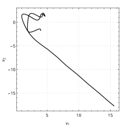
Figure 1: Parametric plot of $v$ per example 1.

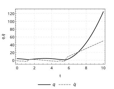
(a)

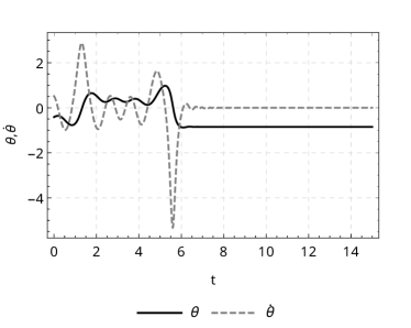
(b)

Figure 2: Radial and angular components of $v$ per example 1.

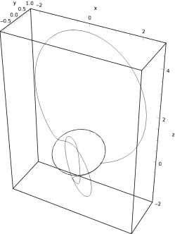
Figure 3: Components of $\widetilde{x}$ projected into $\mathbb{R}^{3}$ per example 1.

Example 2

Setting $C=0$ can yield just as interesting dynamics as $C\neq 0$. The following figures show $v$ as per equations (20) with $v_{1}(0)=2,v_{2}(0)=-1,\dot{v}_{1}(0)=2,\dot{v}_{2}(0)=-1,\ddot{v}_{1}(0)=0$ and $\ddot{v}_{2}(0)=5$.

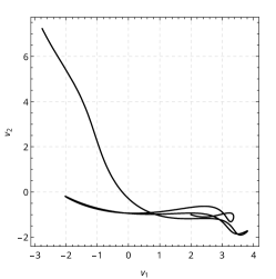
Figure 4: Parametric plot of $v$ per example 2.

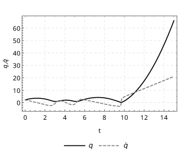
(a)

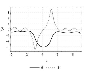
(b)

Figure 5: Radial and angular components of $v$ per example 2.

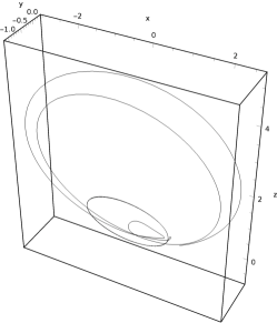
Figure 6: Components of $\widetilde{x}$ projected into $\mathbb{R}^{3}$ per example 2.

References

• Camarinha et al. (2001) M. Camarinha, F. S. Leite,  and P. Crouch, Differential Geometry and its Applications 15, 107 (2001).
• Pauley and Noakes (2012) M. Pauley and L. Noakes, Differential Geometry and its Applications 30, 694 (2012).
• GiambA et al. (2002) R. GiambA, F. Giannoni,  and P. Piccione, IMA Journal of Mathematical Control and Information 19, 445 (2002).
• Noakes (2003) L. Noakes, Journal of Mathematical Physic 44, 1436 (2003).
• Noakes and Ratiu (2016) L. Noakes and T. Ratiu, Communications in Mathematical Sciences 14 (2016).
• Noakes (2006a) L. Noakes, Advances in Computational Mathematics 25, 195 (2006a).
• Montgomery (2006) R. Montgomery, A Tour of Subriemannian Geometries, Their Geodesics and Applications (American Mathematical Society, 2006).
• L. S. Pontryagin, V. G. Boltyanskii, R. V. Gamkrelidze, E. F. Mishechenko (1963) L. S. Pontryagin, V. G. Boltyanskii, R. V. Gamkrelidze, E. F. Mishechenko, Journal of Applied Mathematics and Mechanics 43, 514 (1963).
• Sachkov (2009) Y. Sachkov, Journal of Mathematical Sciences 156, 381 (2009).
• Noakes (2006b) L. Noakes, The Quarterly Journal of Mathematics 57, 527 (2006b).
• Noakes (2008) L. Noakes, Siam Journal on Applied Dynamical Systems 7, 437 (2008).