Electro-optical properties of Cu₂O in the regime of Franz-Keldysh oscillations

Abstract

We present the analytical method enables one to compute the optical functions i.e., reflectivity, transmission and absorption including the excitonic effects for a semiconductor crystal exposed to a uniform electric field for energy region above the gap, for external field suitable to appearance of Franz-Keldysh (FK) oscillations. Our approach intrinsically takes into account the coherence between the carriers and the electromagnetic field. We quantitatively describe the amplitudes and periodicity of FK modulations and the influence of Rydberg excitons on FK effect is also taking into account. Our analytical findings are illustrated numerically for $P$ excitons in Cu₂O crystal.

I Introduction

The absorption of light at the fundamental gap in semiconductors reveals two different kinds of electronic transitions. At photon energies greater than the energy gap the absorption of light causes processes in which an electron is transferred to the conduction band and a hole is left in the valence band. At energies lower than the gap there are absorption peaks which correspond to processes in which the conduction band electron and the valence hole are bound to one another in states within the forbidden energy gap. The possibility that electrons can exist in semiconductors in excited bound states, termed excitons, was first suggested by Frenkel Frenkel and Peierls Peierls more than 80 year ago. In analogy to the tight binding and the nearly free electron approximations, two types of excitons are considered: tightly bound (Frenkel excitons) and weakly bound (Wannier-Mott excitons). Frenkel excitons have a Bohr radius of the order of the lattice constant or smaller. Such exciton is strongly bound and usually localized on one site. The electron and the hole do not move independently. In contrast, the Bohr radius of a Wannier-Mott exciton is much larger than the lattice constant, therefore it has a smaller binding energy and is delocalized over a number of sites. Below we deal with the weakly bound excitons. In 1952, E. Gross and N. Karriev Gross discovered these Wannier-Mott excitons experimentally in a copper oxide (Cu₂O) semiconductor. After that time excitons have remained an important topic of experimental and theoretical research, because of their dominant role on the optical properties of semiconductors (molecular crystals etc.,). The excitons have been studied in great details in various types of semiconductor nanostructures and in bulk crystals. Since there is a inestimable number of papers, monographs, review articles devoted to excitons, we refer to only a small collection of them. Knox ^-Klingshirn In 80-ties of the last century the main stream of research on excitons was focussed on III-V and II-VI semiconductors, but the research on the properties of excitons in Cu₂O was continued, in particular, by the group of Dortmund (Froelich and the references therein).

A lot of studies, both experimental and theoretical, have been devoted to examine various properties of excitons in Cu₂O bulk crystal and it appeared that the spectroscopical features of copper oxide are through-out recognized (see Refs.Froelich ^-Stolz_2012 ). But recently, the interest on this bulk semiconductor has reborn due to outstanding experiment performed by Kazimierczuk et al.Kazimierczuk who discovered highly excited states, so-called Rydberg excitons (RE) in the natural crystal of copper oxide. They have observed absorption lines associated with excitons of principal quantum numbers up to $n=25$.

A large amount of new studies which focused on extraordinary properties of RE attracted increasing attention during last three years (Thewes ^-Walther ), especially on their behaviour in external fieldsZielinska.PRB.2016.b ^-Zielinska.PRB.2016.c as well as in the context of their spectra similarity to quantum chaos and breaking of all antiunitary symmertiesAssmann_symmetry ^-Schweiner_Symmetry . Recently the first observation of photoluminescence of excitonic Rydberg states has been reported kitamura .

Up till now much effort has been devoted to examine excitons in Cu₂O for energies below the gap, the region in which the most important effect, i.e. the appearance of excitons with high number $n$, has been observed. One of the distinction peculiarity of copper oxide is the moderately small Rydberg energy of only 90 meV, which assures that all of relevant states from the ground state up to the continuum above the band gap are optically accessible using attainable lasers.

Recently some attempts Hecktoetter_2017 have been reported , where the optical properties of Cu₂O for excitation energies exceeding the fundamental gap, are examined. Hecktötter et al., Hecktoetter_2017 using two-color pump-probe spectroscopy, studied RE in copper oxide in the presence of free carriers injected by above-band-gap excitation. They examined the impact of an ultra-low-density plasma on Rydberg excitations at the temperature of a few Kelvin and observed that inside a Cu₂O crystal plasma shifts the band edge downwards, diminishing the maximum excitable Rydberg state which, in consequence, leads to modulation of plasma blockade induced by the band gap modulation.

Below we study an another effect appearing for above-gap excitation, which refers to electro-optic properties. For excitation energies below the gap, the main electro-optic effects are the shifting, splitting, and, for higher excitonic states, mixing of spectral lines.Zielinska.PRB.2016.b As it was observed for direct-band semiconductors, for energies above the gap and when a constant electric field is applied, specific oscillations in the spectra has been observed, known as the Franz-Keldysh oscillations. Franz ^-Lee

These oscillations are results of wave functions ”leaking” into the band gap; the key mechanism of this effect is photon-assisted tunnelling across the bandgap. When an electric field is applied, the electron and hole wave functions become Airy functions rather than plane waves (and they have a ”tail” which extends into the classically forbidden band gap). Due to an electric field influence on interband transitions in the presence of excitons the dielectric constant of a semiconductor exhibits Franz-Keldysh oscillations (FKO), which can be detected by modulated reflectance. Franz-Keldysh effect, which gives the possibility to create and control reflectivity oscillations, provide a key ingredient to the goal of achieving a precise tool for steering on-demand periodicity and amplitude of electro-modulations. FK effect has found also practical applications, see, for example, patents.Patent

The theoretical description of the FK effect is quite different of all phenomena below the gap. For energies below gap a well known solution of a hydrogen-like Schrödinger equation can be used, where the term related to the applied electric field is treated as a perturbation.Zielinska.PRB.2016.b For energies above the gap one deals with the continuum states. When the electric field is applied, the relevant material (constitutive) equation contains terms of different symmetry, so an analytical solution is not known.

As it was mentioned by Ralph Ralph many years ago, to the best of our knowledge, up till now the FK effect was not examined for the Cu₂O bulk crystal. In this paper we propose modification of the real density matrix approach which was applied in our the previous papersZielinska.PRB ; Zielinska.PRB.2016.b ; Zielinska.PRB.2016.c to describe optical properties of Rydberg excitons below gap. Here we develop this approach including energies above the gap and taking into account the changes caused by an externally applied electric field, which intensity should be small enough to avoid Stark localization but on the other hand sufficient to enable observation of Franz-Keldysh oscillations. Franz-Keldysh effect gives the possibility to create and control reflectivity oscillations. Circumventing this problem would be a key to achieve the goal to a precise tool for steering on-demand periodicity and amplitude of electro-modulations.

Below we show that using excitons one gets a flexible tool to study the oscillation dynamics of reflectivity of a Cu₂O crystal irradiated by an electromagnetic radiation and affected by an electric field. The tunability, which can be exploited to force the desired period and amplitude of modulations, can be achieved through the modification of an external electric field intensity, which in turn influences the excitonic levels shifting and overlapping.

The paper is organized as follows. In Sec. II we sketch the outline and present general density matrix equations governing the evolution of the system, necessary for calculation of the macroscopic polarization of a medium. This general considerations are then specified for the case of Cu₂O in Sec. III. In Sec. IV the electro-susceptibility is studied for the case of $P$-exciton. Sections V and VI contain the discussion how more excitonic states can be accounted for in the calculations of the FK effect. The analytical expression for the transmissivity is presented in Sec. VII and illustrative examples of susceptibility for Cu₂O are examined. The conclusions are discussed in the last section VIII.

II Density matrix formulation

We intend to calculate the optical functions of a Cu₂O crystal, when a homogeneous electric field is applied in the $z$ direction, which is chosen to be perpendicular to the crystal surface, and the excitation energy exceeds the fundamental gap energy. The method is based on the so-called real density matrix approach (RDMA) which, for a similar physical situation, but with excitation energy below the gap, was used in Ref.Zielinska.PRB.2016.b The kernel of the RDMA is the so-called constitutive equation

$$\dot{Y}(\textbf{R},\textbf{r})+({i}/\hbar)H_{eh}{Y}(\textbf{R},\textbf{r})+(1/\hbar){\mit\Gamma}{Y}(\textbf{R},\textbf{r})$$

$$=({\rm i}/\hbar)\textbf{M}(\textbf{r})\textbf{E}(\textbf{R}),$$ (1)

where $Y$ is the bilocal coherent electron-hole amplitude (pair wave functions), ${\bf R}$ is the excitonic center-of-mass coordinate, $\textbf{r}=\textbf{r}_{e}-\textbf{r}_{h}$ the relative coordinate, $\textbf{M}(\textbf{r})$ the smeared-out transition dipole density, ${\bf E}({\bf R})$ is the electric field vector of the wave propagating in the crystal. The coefficient $\mit\Gamma$ in the constitutive equation represents dissipative processes. The two-band effective mass Hamiltonian $H_{eh}$ of the system under a constant electric field $\textbf{F}=(0,0,F)$ that includes the electron- and hole kinetic energy terms, the electron-hole interaction potential and the confinement potentials Zielinska.PRB has the form

$$H_{eh} = E_{g}-\frac{\hbar^{2}}{2m_{e}}\partial^{2}_{z_{e}}-\frac{\hbar^{2}}{2m_{hz}}\partial^{2}_{z_{h}}-\frac{\hbar^{2}}{2\mu_{\parallel}}(\partial^{2}_{x}+\partial^{2}_{y})$$

$$-\frac{\hbar^{2}}{2M_{\parallel}}\left(\partial^{2}_{R_{\parallel}}+R^{-1}_{\parallel}\partial_{R_{\parallel}}\right)+eF(z_{h}-z_{e})$$

$$+V_{eh}(z_{e}-z_{h},\rho)+V_{e}(z_{e})+V_{h}(z_{h}),$$

where we have separated the center-of-mass coordinate $R_{\parallel}$ from the relative coordinate $\rho$ on the plane $x-y$.

The dipole density vectors M should be chosen appropriate for P- or F- excitons. Zielinska.PRB.2016.c The potential term representing the Coulomb interaction in an anisotropic medium is given by

$$V_{eh}=-\frac{e^{2}}{4\pi\epsilon_{0}\epsilon_{b}[(x^{2}+y^{2})+z^{2}\epsilon_{\parallel}/\epsilon_{z}]^{1/2}},$$ (3)

where we introduce the two effective dielectric constants, $\epsilon_{\parallel}$, and $\epsilon_{z}$, respectively, and define $\epsilon_{b}=\sqrt{\epsilon_{\parallel}\epsilon_{z}}$. The smeared-out transition dipole density ${\bf M}({\bf r})$, should be chosen in our case appropriate for P- or F- excitons, Zielinska.PRB.2016.c is related to the bilocality of the amplitude $Y$ and describes the quantum coherence between the macroscopic electromagnetic field and the interband transitions.

The coherent amplitude $Y$ defines the excitonic counterpart of the polarization

$$\textbf{P}(\textbf{R})=2\int{\rm d}^{3}r~{}\hbox{Re}~{}\left[\textbf{M}(\textbf{r})Y(\textbf{R},\textbf{r})\right],$$ (4)

which is than used in the Maxwell propagation equation

$$c^{2}\nabla_{R}^{2}\textbf{E}-\underline{\underline{\epsilon}}_{b}\ddot{\textbf{E}}(\textbf{R})=\frac{1}{\epsilon_{0}}\ddot{\textbf{P}}(\textbf{R}),$$ (5)

with the use of the bulk dielectric tensor $\underline{\underline{\epsilon}}_{b}$ and the vacuum dielectric constant $\epsilon_{0}$. In the present paper we solve the eqs. (II)-(5) in order to compute the electro-optical functions (i.e.,reflectivity, transmission, and absorption) for Cu₂O. Contrary to the previous paper on electro-optical properties Zielinska.PRB.2016.b we will consider the excitation energies above the energy gap, which will require a different approach.

Both polarization and electric field must obey Maxwell‘s equations, which have to be solved in order to get the propagation modes. The above approach takes into account key factors necessary for the calculation of all optical functions. They are obtained, as usual, by comparing the amplitudes of incident, reflected or transmitted electric fields, and depend on the applied field strength and on the total crystal thickness.

III The basic equations

The considered crystal is modelled by a slab with infinite extension in the $xy$-plane and the boundary planes $z=0,z=L$. With the sake of simplicity, the slab is located in vacuum. An monochromatic, linearly polarized electromagnetic wave propagates along $z$ axis. Its electric field is given by

$${\bf E}=(0,E_{y},0),\qquad E_{y}=E_{in}e^{{i}k_{0}z-{i}\omega t}\,,$$ (6)

where $k_{0}={\omega}/{c}$ is the wave vector in the vacuum with $\omega$ being the frequency and $E_{in}$ is an amplitude of the incoming wave. Due to the fact that the energy of the propagating wave is divided into reflected and transmitted wave one obtains the reflectivity, transmissivity and absorption from the relations

$$R=\left|\frac{E(0)}{E_{in}}-1\right|^{2}, T=\left|\frac{E(z=L)}{E_{in}}\right|^{2},$$

$$A = 1-R-T,$$ (7)

where $E(z)$ is the $x$-component of the wave electric field inside the crystal. The calculation of the optical functions consists of several steps. The first one is the solution of the constitutive equation (II). Due to the specific properties of Cu₂O, we will treat the crystal as the bulk region and look for the amplitude $Y$ in the form

$$Y(Z,\textbf{r})=Y(\textbf{r})e^{{i}k_{z}Z}.$$ (8)

Assuming the wave propagation in the $z$ direction, we neglect the $R_{\parallel}$ component and arrive at the equation

$$\big{[}E_{g}-\hbar\omega-{i}{\mit\Gamma}+\frac{\hbar^{2}k_{z}^{2}}{2M_{z}}-\frac{\hbar^{2}}{2\mu_{z}}\partial^{2}_{z}-\frac{\hbar^{2}}{2\mu_{\parallel}}\left(\partial^{2}_{x}+\partial^{2}_{y}\right)$$

$$+eFz+V_{eh}(z,\rho)\big{]}Y(x,y,z)=\textbf{M}({\bf r})\textbf{E}(Z),$$ (9)

where $M_{z},\mu_{z}$ are the exciton total and reduced effective masses in the $z$-direction, respectively. For further considerations we must specify the dipole density $M$. Due to symmetry properties of Cu₂O the total symmetry of the excitons‘ state must be the same as the symmetry of the dipole operator, and according to this the transition dipole density appropriate for $P$ exciton will be considered. This will result in the shapes of the real and imaginary part of the electro-susceptibility. In the previous papers,Zielinska.PRB.2016.b ^,Zielinska.PRB.2016.c for energies below the gap, we took the dipole density in terms of spherical coordinates. For energies above the gap and with the applied electric field, the cylindrical symmetry must be used. For the sake of simplicity, we use the in-plane components of the dipole density with the coherence radius $r_{0}$ along the planes and zero in the growth direction. The cylindrical version of the formulas for $M_{x}$ and $M_{y}$ components, given in ref. Zielinska.PRB.2016.c , has the form

$${M}_{x}^{(1)} \propto {M}_{0}\sqrt{x^{2}+y^{2}}\left(e^{{i}\phi}-e^{-{i}\phi}\right)\frac{\exp[-\frac{x^{2}+y^{2}}{2r^{2}_{0}}]}{{i}\sqrt{\pi}r^{3}_{0}}\delta(z),$$

$${M}_{y}^{(1)} \propto {M}_{0}\sqrt{x^{2}+y^{2}}\left(e^{{i}\phi}+e^{-{i}\phi}\right)\frac{\exp[-\frac{x^{2}+y^{2}}{2r^{2}_{0}}]}{\sqrt{\pi}r^{3}_{0}}\delta(z).$$

For further considerations we introduce dimensionless quantities

$$\rho=\frac{\sqrt{x^{2}+y^{2}}}{a^{*}},\quad\zeta=\frac{z}{a^{*}{\sqrt{\gamma}}},$$ (11)

$$f=\frac{F}{F_{\rm{I}}},$$

$$k^{2}=\frac{2\mu_{\parallel}}{\hbar^{2}}a^{*2}\left(E_{g}-{\hbar}{\omega}-{\rm i}{\mit\Gamma}\right)+\frac{\mu_{\parallel}}{M_{z}}\left(k_{z}^{2}a^{*2}\right),$$

where $F_{\rm{I}}$ is the so-called ionization field

$$F_{\rm{I}}=\frac{\hbar^{2}}{2\mu_{\parallel}ea^{*3}}=\frac{R^{*}}{a^{*}e},$$ (12)

with excitonic Rydberg $R^{*}$, $a^{*}$ being the corresponding excitonic Bohr radius, and the anisotropy parameter $\gamma=\mu_{\parallel H}/\mu_{z}$. With these quantities the Eq. (III) can be rewritten in the form

$$\left(k^{2}-\partial^{2}_{\rho}-\frac{1}{\rho}\partial_{\rho}-\frac{1}{\rho^{2}}\partial^{2}_{\phi}-\partial^{2}_{\zeta}+f\sqrt{\gamma}{\zeta}\right)Y$$

$$=\frac{2\mu_{\parallel}}{\hbar^{2}}a^{*2}M^{(1)}E_{y}+\frac{2}{\sqrt{\rho^{2}+{\gamma}{\zeta^{2}}}}Y.$$ (13)

$M^{(1)}$ denotes the relevant components ($x$ or $y$) of the dipole density and $E_{y}$ is the $y$ component of electric wave field.

IV The electro-susceptibility for the $P$ exciton

In this section we derive the expression for the bulk Cu₂O electro-susceptibility for $P$ exciton. Following the procedure described in Ref. Dressler , we separate the hamiltonian of Eq. (II) transformed to the form (III) into a ’’kinetic+electric field‘‘ part $H_{\rm{kin+F}}$ and a potential term $V$ which lead to the following form of the basic constitutive equations (II)

$$H_{\rm{kin}+F}Y={\bf M}{\bf E}-VY.$$ (14)

The above expression corresponds to Lippmann-Schwinger equation, in which the Green function $G$ appropriate to the ’’kinetic+electric field‘‘ part is adopted for the coherent amplitude

$$Y=G{\bf M}{\bf E}-GVY.$$ (15)

The Green function for Eq. (III) has the form

$$G(\rho,\rho^{\prime};\zeta,\zeta^{\prime};\phi,\phi^{\prime})=\frac{1}{(f\sqrt{\gamma})^{\frac{1}{3}}}$$ (16)

$$\times\frac{1}{2\pi}\sum\limits_{m=-\infty}^{\infty}e^{{\rm i}m(\phi-\phi^{\prime})}\int\limits_{0}^{\infty}x\,{\rm d}x\,J_{m}(x\rho)J_{m}(x\rho^{\prime})g_{x}(\zeta,\zeta^{\prime}),$$

where

$$g_{x}(\zeta,\zeta^{\prime})=g^{<}\;g^{>},$$

$$g^{<}=\pi{\rm Bi}\left[(f\sqrt{\gamma})^{\frac{1}{3}}\left(\zeta^{<}+\frac{k^{2}+x^{2}}{f\sqrt{\gamma}}\right)\right]$$

$$+{i}{\rm Ai}\left[(f\sqrt{\gamma})^{\frac{1}{3}}\left(\zeta^{<}+\frac{k^{2}+x^{2}}{f\sqrt{\gamma}}\right)\right],$$ (17)

$$g^{>}={\rm Ai}\left[(f\sqrt{\gamma})^{\frac{1}{3}}\left(\zeta^{>}+\frac{k^{2}+x^{2}}{f\sqrt{\gamma}}\right)\right],$$

$J_{m}$ are Bessel functions, and $\rm{Ai}(z)$, $\rm{Bi}(z)$ are Airy functions (see Ref.Abram81 ).

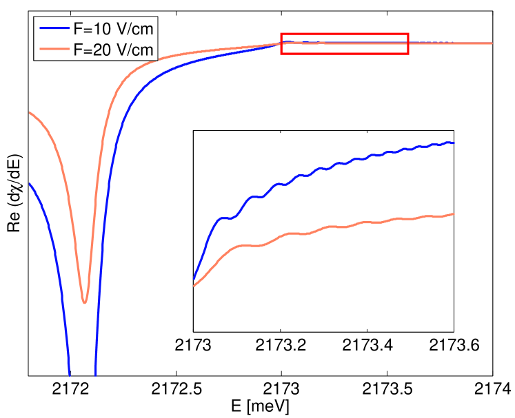
Figure 1: Real part of the electro-susceptibility for a Cu₂O crystal, calculated by the formula (IV), taking into account the excitonic effect, for two values of the electric-field strength ($F$=10 V/cm and $F$=20 V/cm), with the coherence radius $\rho_{0}=0.2~{}a^{*}$, $\Gamma=0.05$ meV.

To obtain the optical functions one has to solve the Eq. (15) using the Green function (16). Please note that the Eq. (15) has the form of Fredholm integral equation of second type. There are many methods of solving such equations Analysis and particular choice depends on specific properties of the particular crystal. One of the methods uses a certain form of the function $Y$ (ansatz) which depends on an unknown parameter $Y_{0}$. The parameter is then obtained from the equation (15) and used to calculate the polarization from Eq. (4) and the electric field of the wave from Eq. (5).

The ansatz for $Y$ will be taken in the form

$$Y(\rho,\zeta,\phi)=Y_{0}\frac{e^{{i}\phi}+e^{-{i}\phi}}{2}\,\rho\exp\left(-k\sqrt{\rho^{2}+\gamma\zeta^{2}}\right).$$ (18)

which has the symmetry of 2P exciton state. With the above ansatz, Green‘s function (16) and the $M_{y}$ dipole densities (III), which in our scaled variables (normalized in spatial variables $\rho,\zeta$) takes the form

$$M_{y}^{(1)} = \sqrt{\frac{2}{\pi}}\frac{M_{0}}{\pi\sqrt{\gamma}\rho^{3}_{0}a^{*3}}$$ (19)

$$\times\rho\,\exp\left(-\frac{\rho^{2}}{2\rho^{2}_{0}}\right)\frac{e^{{\rm i}\phi}+e^{-{i}\phi}}{2}\delta(\zeta),$$

where $\rho_{0}=r_{0}/a^{*}$, we obtain the following expression for the susceptibility

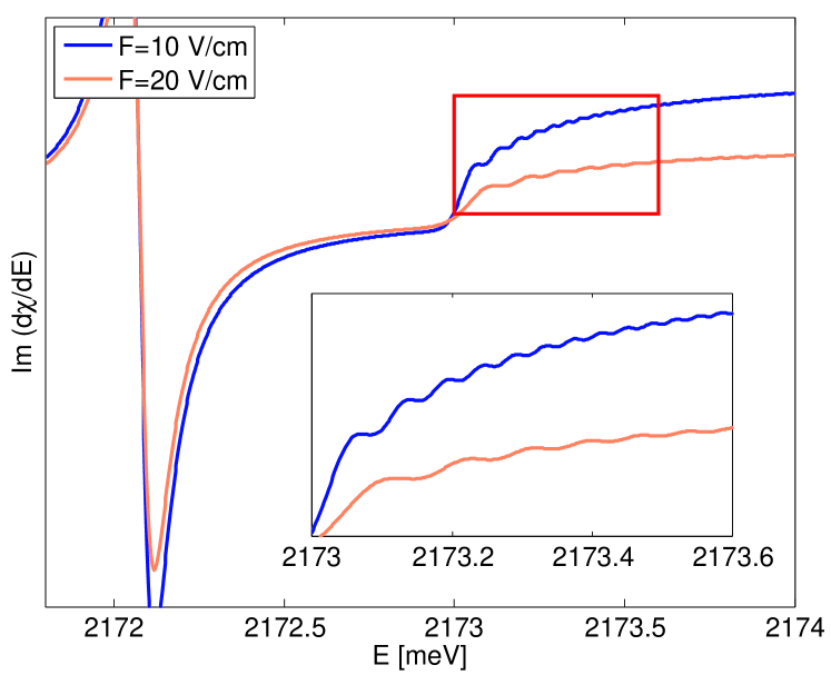
Figure 2: The same as in Fig. 1, for the imaginary part of the susceptibility

$$\chi=2\frac{|M_{0}|^{2}2\mu_{\parallel}\rho_{0}^{2}}{\epsilon_{0}\sqrt{\gamma}a^{*}\hbar^{2}(f\sqrt{\gamma})^{\frac{1}{3}}Q}$$

$$\times\int\limits_{0}^{\infty}x^{3}{\rm d}x\exp(-\rho_{0}^{2}x^{2})\biggl{[}\mbox{Bi}\left(\frac{k^{2}_{x}}{(f\sqrt{\gamma})^{\frac{2}{3}}}\right)$$ (20)

$$+{i}\mbox{Ai}(\frac{k^{2}_{x}}{(f\sqrt{\gamma})^{\frac{2}{3}}})\biggr{]}\mbox{Ai}\left(\frac{k^{2}_{x}}{(f\sqrt{\gamma})^{2/3}}\right)\frac{\tilde{M}Y}{M_{0}Y_{0}}$$

$$=2\frac{|M_{0}|^{2}2\mu_{\parallel}\rho_{0}^{2}}{\epsilon_{0}\sqrt{\gamma}a^{*}\hbar^{2}Q}\cdot\frac{1}{2}(f\sqrt{\gamma})e^{-\mathcal{E}\rho_{0}^{2}}$$

$$\times\int\limits_{-\mathcal{E}}^{\infty}{\rm d}u\,e^{-\rho_{0}^{2}(f\sqrt{\gamma})^{2/3}u}\left(u+{\mathcal{E}}\right)\left[\mbox{Bi}(u)+i\mbox{Ai}(u)\right]\hbox{Ai}(u),$$

and

$$k^{2}_{x}=k^{2}+x^{2},$$

$$u=\frac{k^{2}+x^{2}}{(f\sqrt{\gamma})^{2/3}},$$

$$\hbar\Theta=R^{*}(f\sqrt{\gamma})^{2/3}=\left(\frac{\hbar^{2}}{2\mu_{z}}\right)^{1/3}(eF)^{2/3},$$ (21)

$${\mathcal{E}}=\frac{\hbar\omega-E_{g}}{\hbar\Theta},$$

$$\frac{\tilde{M}Y}{M_{0}Y_{0}}=\frac{\sqrt{2\pi}}{\sqrt{\gamma}}\rho_{0}\exp\left(\frac{k^{2}\rho_{0}^{2}}{4}\right)D_{-4}(k\rho_{0}),$$

$\hbar\Theta$ being the so-called electro-optical energy, and $D_{-4}$ the parabolic cylinder function (for example, Abram81 ^, Grad )

$$D_{p}(z)=\frac{\exp(-z^{2}/4)}{\Gamma(-p)}\int\limits_{0}^{\infty}e^{-xz-(x^{2}/2)}x^{-p-1}{\rm d}x,$$

$$\qquad(\hbox{Re}\,p<0).$$ (22)

The expression $Q$ appearing in the denominator in (IV) is given by

$$Q=\frac{(\tilde{M}Y)-\tilde{M}GVY}{M_{0}Y_{0}},$$ (23)

where

$$\frac{\tilde{M}GVY}{M_{0}Y_{0}}=\frac{2\pi}{(f\sqrt{\gamma})^{1/3}}\int\limits_{0}^{\infty}{x^{3}\,{\rm d}x}e^{-\rho^{2}_{0}x^{2}/2}\mbox{Ai}\left(\frac{k^{2}_{x}}{(f\sqrt{\gamma})^{2/3}}\right)$$

$$\times\int\limits_{0}^{\infty}{\rm d}\zeta\left(\frac{\sqrt{\gamma}\zeta}{k_{x}^{2}}+\frac{1}{k_{x}^{3}}\right)e^{-k_{x}\sqrt{\gamma}\zeta}\biggl{\{}\mbox{Bi}\left[(f\sqrt{\gamma})^{1/3}\left(\frac{k^{2}_{x}}{f\sqrt{\gamma}}-\zeta\right)\right]$$

$$+{i}\mbox{Ai}((f\sqrt{\gamma})^{1/3}\left(\frac{k^{2}_{x}}{f\sqrt{\gamma}}-\zeta)\right)\biggr{\}}$$

$$+\frac{2\pi}{(f\sqrt{\gamma})^{1/3}}\int\limits_{0}^{\infty}{x^{3}\,{\rm d}xe^{-\frac{\rho^{2}_{0}x^{2}}{2}}}\biggl{[}\mbox{Bi}\left(\frac{k^{2}_{x}}{(f\sqrt{\gamma})^{2/3}}\right)$$ (24)

$$+{i}\mbox{Ai}\left(\frac{k^{2}_{x}}{(f\sqrt{\gamma})^{2/3}}\right)\biggr{]}$$

$$\times\int\limits_{0}^{\infty}{\rm d}\zeta e^{-k_{x}\sqrt{\gamma}\zeta}\left(\frac{\sqrt{\gamma}\zeta}{k_{x}^{2}}+\frac{1}{k_{x}^{3}}\right)\mbox{Ai}\left[(f\sqrt{\gamma})^{1/3}\left(\frac{k^{2}_{x}}{f\sqrt{\gamma}}+\zeta\right)\right].$$

The vanishing of the real part gives the resonance of the susceptibility. In particular, for the case without electric field $F=0$, one obtains

$$\frac{\tilde{M}GVY}{M_{0}Y_{0}}=\frac{1}{3k}\sqrt{\frac{2}{\pi}}\frac{1}{\sqrt{\gamma}}\frac{2(1+2\sqrt{\gamma})}{(1+\sqrt{\gamma})^{2}}e^{k^{2}\rho_{0}^{2}/4}\Gamma(4)D_{-4}(k\rho_{0}),$$ (25)

with the Euler Gamma function $\Gamma(z)$. Some unique features of the susceptibility can be read off directly from the formula (IV). In particular, for energies above the gap (i.e. for $\hbar\omega>E_{g}$) we obtain the FK oscillations in the spectrum, which appear due to periodical character of Airy functions Ai and Bi.

Some quantitative properties of the spectrum can be obtained by neglecting the electron-hole interaction, i.e. by taking $V=0$. The results for the susceptibility ensue from the formula (IV) with $Q=1$ are shown in Fig.1 (the real part) and Fig. 2 (the imaginary part) for two values of the applied electric field and two values of $\rho_{0}$. We have used the values $E_{g}=2172~{}\hbox{meV},R^{*}=86.981~{}\hbox{meV}$, $\gamma=0.5351$, $\mu_{\parallel}=0.396\;m_{0},a^{*}=1.0\;\hbox{nm}$, and phenomenological value of damping ${\mit\Gamma}=0.05~{}\hbox{meV}$. The dipole matrix element $M_{0}$ is related to the longitudinal-transverse splitting energy $\Delta_{LT}$.Zielinska.PRB

It can be seen from Fig.1-2 that for energies above the gap the noticeable oscillations in dispersion and absorption spectra appear. Their period and amplitude increase with a fields strength. It should be noted that the external field should be chosen carefully, i.e., to be small enough to avoid Stark localization but sufficiently strong for oscillation to manifest. The results of the field impact is more pronounced on susceptibility differential spectrum

$$\Delta\chi=\chi(F)-\chi(F=0).$$ (26)

Fig. 3 presents the imaginary part of the susceptibility for two values of the external electric fields. One can see more explicit the oscillations of real and imaginary part of $\chi$; their amplitudes are slightly dependent on the the field strength while oscillation period strongly depends on the field; this relation will be discussed in more details below.

The results are more evident when we consider the limit ${\mit\Gamma}\to 0,k_{z}\to 0,\rho_{0}\to 0$, which is suitable for situation above the gap. Then the integrals in (IV) involving Airy functions can be performedAiry and we obtain

$$\mbox{Re}\,\chi=\frac{4\chi^{\prime}\sqrt{\pi}\rho_{0}^{3}}{Q}\left(\frac{\hbar\Theta}{R^{*}}\right)^{3/2}$$

$$\times\frac{1}{6}\left[4{\mathcal{E}}\hbox{Ai}^{\prime}\hbox{Bi}^{\prime}+4{\mathcal{E}}^{2}\hbox{Ai}\hbox{Bi}-\hbox{Ai}^{\prime}\hbox{Bi}-\hbox{Ai}\hbox{Bi}^{\prime}\right]$$ (27)

$$=\frac{4\chi^{\prime}\sqrt{\pi}\rho_{0}^{3}}{Q}\biggl{\{}\frac{2}{3}\left(\frac{\hbar\Theta}{R^{*}}\right)^{1/2}$$

$$\times\left(\frac{\hbar\omega-E_{g}}{R^{*}}\right)\hbox{Ai}^{\prime}\left(-\frac{\hbar\omega-E_{g}}{\hbar\Theta}\right)\hbox{Bi}^{\prime}\left(-\frac{\hbar\omega-E_{g}}{\hbar\Theta}\right)$$

$$+\frac{2}{3}\left(\frac{R^{*}}{\hbar\Theta}\right)^{1/2}\left(\frac{\hbar\omega-E_{g}}{R^{*}}\right)^{2}$$

$$\times\hbox{Ai}\left(-\frac{\hbar\omega-E_{g}}{\hbar\Theta}\right)\hbox{Bi}\left(-\frac{\hbar\omega-E_{g}}{\hbar\Theta}\right)$$

$$-\frac{1}{6}\left(\frac{\hbar\Theta}{R^{*}}\right)^{3/2}\hbox{Ai}^{\prime}\left(-\frac{\hbar\omega-E_{g}}{\hbar\Theta}\right)\hbox{Bi}\left(-\frac{\hbar\omega-E_{g}}{\hbar\Theta}\right)$$

$$-\frac{1}{6}\left(\frac{\hbar\Theta}{R^{*}}\right)^{3/2}\hbox{Ai}\left(-\frac{\hbar\omega-E_{g}}{\hbar\Theta}\right)\hbox{Bi}^{\prime}\left(-\frac{\hbar\omega-E_{g}}{\hbar\Theta}\right)\biggr{\}}$$

$$\hbox{Im}\,\chi=-C\biggl{\{}\frac{1}{6}\left(\frac{\hbar\Theta}{R^{*}}\right)^{3/2}\hbox{Ai}^{\prime}\left(-\frac{\hbar\omega-E_{g}}{\hbar\Theta}\right)\hbox{Ai}\left(-\frac{\hbar\omega-E_{g}}{\hbar\Theta}\right)$$

$$+\frac{1}{3}\left(\frac{\hbar\Theta}{R^{*}}\right)^{1/2}\left(\frac{\hbar\omega-E_{g}}{R^{*}}\right)\hbox{Ai}^{\prime 2}\left(-\frac{\hbar\omega-E_{g}}{\hbar\Theta}\right)$$

$$+\frac{1}{3}\left(\frac{R^{*}}{\hbar\Theta}\right)^{1/2}\left(\frac{\hbar\omega-E_{g}}{R^{*}}\right)^{2}\hbox{Ai}^{2}\left(-\frac{\hbar\omega-E_{g}}{\hbar\Theta}\right)\biggr{\}}$$ (28)

with a certain constant C, and $\chi^{\prime}$ defined as

$$\chi^{\prime}=\frac{\epsilon_{b}\sqrt{\pi}\Delta_{LT}}{8R^{*}\sqrt{\gamma}{\rho_{0}}}.$$

Note that the above expressions differ from the expressions for S-excitons (allowed interband transitions, for example GaAs)Tharmalingam ; callaway ; Dressler

$$\hbox{Im}\,\chi\propto\biggl{\{}\frac{\hbar\omega-E_{g}}{\hbar\Theta}\hbox{Ai}^{2}\left(-\frac{\hbar\omega-E_{g}}{\hbar\Theta}\right)$$

$$+\left[\hbox{Ai}^{\prime}\left(-\frac{\hbar\omega-E_{g}}{\hbar\Theta}\right)\right]^{2}\biggr{\}}.$$ (29)

Now we can perform qualitative discussion of the spectra spectra features. Having in mind the properties of Cu₂O we observe, that the value of the electro-optical energy $\hbar\Theta$ is small compared to the Rydberg energy. Therefore the arguments of the Airy functions in expressions (IV) and (IV) quickly reach the values which justify the use of their asymptotic expansions, giving in the lowest order with respect to $\zeta$ the formulas for the real and imaginary part of the susceptibility

$$\hbox{Re}\,\chi\to C_{1}\left(\frac{\hbar\Theta}{R^{*}}\right)^{3/2}\sin 2\zeta,$$ (30)

$$\hbox{Im}\,\chi\to-C_{2}\left(\frac{\hbar\Theta}{R^{*}}\right)^{3/2}\cos 2\zeta+\frac{1}{3\pi}\left(\frac{\hbar\omega-E_{g}}{R^{*}}\right)^{3/2}$$

$$\zeta=\frac{2}{3}\left(\frac{\hbar\omega-E_{g}}{\hbar\Theta}\right)^{3/2},$$

with certain constants $C_{1},C_{2}$. The above expressions allow to get the periodicity of the FK oscillations; the peaks will appear at energies

$$(E_{n}-E_{g})^{{3}/{2}}=\frac{3}{4}n\pi(\hbar\theta)^{3/2}=\frac{3n{\pi}e\hbar F}{4\sqrt{2\mu_{z}}}.$$ (31)

Please note that the above formula includes all extrema. It means that the periodicity of FK oscillations can be used for determining the effective masses along the $z$ axis, as it was done in the case of semiconductor superlattices.Schlichterle ; Nakayama With regard to Eq. (30) we observe FK oscillations around a curve $(\hbar\omega-E_{g})^{3/2}$. The slope is analogous to that obtained for forbidden transitionsTharmalingam ; callaway ; Schaevitz and differs from that observed for $S$ excitons, which in turn depend on $({\hbar\omega-E_{g}})^{1/2}$.Tharmalingam ; callaway ; Dressler

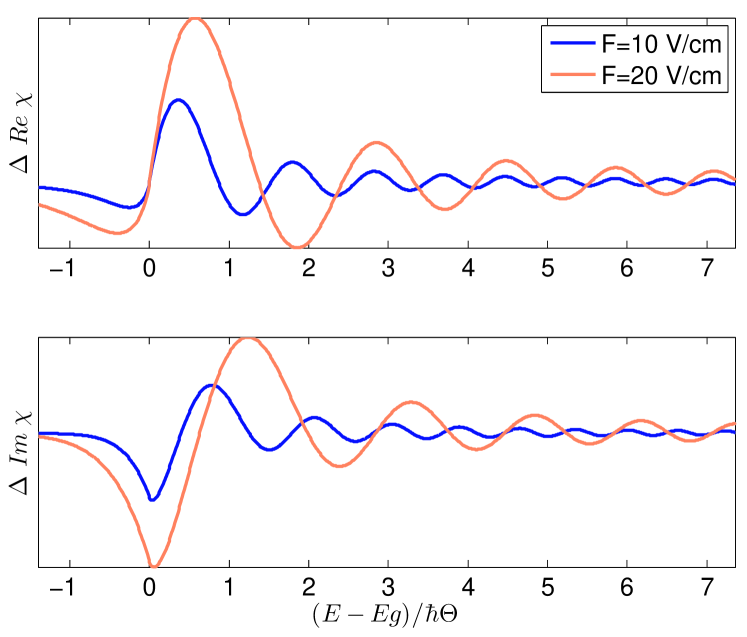
Figure 3: The difference $\Delta\chi=\chi(F)-\chi(F=0)$ displayed for the data of Fig. 1, for two values of the applied electric field.

V Impact of higher excitonic states on Franz-Keldysh effect

Above we have considered the Franz-Keldysh effect with one exciton state. Up till now only the problem of the dependence of multiplicity of excitonic states on Franz-Keldysh effect for confined systems or for a system in an external magnetic field were examined (Festschrift ; RivistaGC and references therein), but the general solution of the issue for bulk crystal is not available. Below we propose a method which allows to study the effect of two lowest exciton states. To achieve this goal we will consider the amplitude $Y$ in the form

$$Y=Y_{1}+Y_{2},$$ (32)

where

$$Y_{1}=N_{1}Y_{01}\rho e^{i\phi}e^{-k\sqrt{\rho^{2}+\gamma^{2}\zeta^{2}}}=Y_{01}\psi_{1},$$

$$Y_{2}=N_{2}Y_{02}\rho e^{i\phi}\left(3-k\sqrt{\rho^{2}+\gamma^{2}\zeta^{2}}\right)e^{-(2k/3)\sqrt{\rho^{2}+\gamma^{2}\zeta^{2}}}$$

$$=Y_{02}\psi_{2},$$ (33)

orthogonal for $k$ real (below the gap for $\Gamma$=0), and $N_{1},N_{2}$ represent the normalization factors for the resonance energies. In the above definitions we neglect the center-of-mass dependence.

The $ansatz$ (32) contains two unknown parameters $Y_{01},Y_{02}$. They can be determined from the integral equation (15). One of the possible methods is to use the projection of those equations onto an orthonormal basis which yields equations for the parameters (Galerkin method). Wee choose the basis in the form

$$\varphi_{1}(\rho,\zeta,\phi) = \frac{1}{\sqrt{\pi}}\frac{\rho}{\rho_{0}^{2}}e^{i\phi}\exp\left(-\frac{\rho^{2}}{2\rho_{0}^{2}}\right)\delta(\zeta),$$ (34)

$$\varphi_{2}(\rho,\zeta,\phi) = \sqrt{\frac{2}{\pi}}\frac{\rho}{\rho_{0}^{2}}e^{i\phi}\left(1-\frac{\rho^{2}}{2\rho_{0}^{2}}\right)\exp\left(-\frac{\rho^{2}}{2\rho_{0}^{2}}\right)\delta(\zeta).$$

Using the common notation for scalar product we obtain two equations

$$\langle\varphi_{1}|Y\rangle = \langle\varphi_{1}|GM\rangle-\langle\varphi_{1}|GVY\rangle,$$

$$\langle\varphi_{2}|Y\rangle = \langle\varphi_{2}|GM\rangle-\langle\varphi_{2}|GVY\rangle,$$ (35)

where we neglected the constant factors. Inserting the expression for $Y$ we get from (V) the equations

$$a_{11}x_{1}+a_{12}x_{2} = b_{1},$$

$$a_{21}x_{1}+a_{22}x_{2} = b_{2},$$ (36)

where

$$x_{1} = \frac{2}{\epsilon_{0}{\mathcal{E}}}M_{0}Y_{01},\quad x_{2}~{}=~{}\frac{2}{\epsilon_{0}{\mathcal{E}}}M_{0}Y_{02},$$

$$a_{11} = \langle\varphi_{1}|\psi_{1}\rangle-\langle\varphi_{1}|G\tilde{V}\psi_{1}\rangle,$$ (37)

and

$$a_{12} = \langle\varphi_{1}|\psi_{2}\rangle-\langle\varphi_{1}|G\tilde{V}\psi_{2}\rangle,$$

$$a_{21} = \langle\varphi_{2}|\psi_{1}\rangle-\langle\varphi_{2}|G\tilde{V}\psi_{1}\rangle,$$

$$a_{22} = \langle\varphi_{2}|\psi_{2}\rangle-\langle\varphi_{2}|G\tilde{V}\psi_{2}\rangle,$$

$$\tilde{V} = \frac{2}{\sqrt{\rho^{2}+\gamma\zeta^{2}}},\qquad\tilde{M}=\frac{M}{M_{0}},$$

$$b_{1} = \frac{2\mu_{\parallel}}{\hbar^{2}a^{*}}\frac{2M_{0}^{2}}{\epsilon_{0}}\langle\varphi_{1}|G\tilde{M}\rangle,$$

$$b_{2} = \frac{2\mu_{\parallel}}{\hbar^{2}a^{*}}\frac{2M_{0}^{2}}{\epsilon_{0}}\langle\varphi_{2}|G\tilde{M}\rangle.$$

The quantities $x_{1},x_{2},b_{1},b_{2}$ are dimensionless; $x_{1},x_{2}$ define the electro-susceptibility by the equation

$$\chi=x_{1}\langle M|\psi_{1}\rangle+x_{2}\langle M|\psi_{2}\rangle.$$ (39)

As it has been done above, some information can be elicit by setting $V=0$. After a simple algebra we obtain

$$x_{1}=\frac{1}{\Delta}\left(b_{1}\langle\varphi_{2}|\psi_{2}\rangle-b_{2}\langle\varphi_{1}|\psi_{2}\rangle\right),$$

$$x_{2}=\frac{1}{\Delta}\left(b_{2}\langle\varphi_{1}|\psi_{1}\rangle-b_{1}\langle\varphi_{2}|\psi_{1}\rangle\right),$$ (40)

$$\Delta=\langle\varphi_{1}|\psi_{1}\rangle\langle\varphi_{2}|\psi_{2}\rangle-\langle\varphi_{1}|\psi_{2}\rangle\langle\varphi_{2}|\psi_{1}\rangle,$$

Comparing the above outcomes with the aforementioned results for one exciton state we observe that an additional state (the same holds for more additional states) will only influence the shape and the amplitude of FK oscillations while the periodicity will practically remain the same since it is involved in the Green function. One can also say that the calculation, at least the analytical one, will be more intricate than in the case of the one exciton state. In consequence, the method described above practically is operational only for two exciton states. However, it should be also stressed that the higher excitonic states are coupled with oscillator strengths decreasing as $1/n^{3}$, so their influence will at least be orders of magnitude smaller that contribution of the two lowest states.

VI Rydberg excitons in a one-dimensional model

As we have discussed above, the simultaneous description of a multiplicity of excitonic states below the gap and the FK oscillations above the gap is, at the moment, not accessible. So, considering the multiplicity of exciton states as the dominant feature of Rydberg excitons, we propose a simplified exciton model, where both phenomena can be described by analytical formulas. To this end, we consider a system with the reduced dimensionality, where the electron with the effective mass $m_{e}$ and the hole with the effective mass $m_{hz}$ move along the $z$-axis. A constant electric field $F$ is applied in the same direction. The optical properties of the system described in previous sections will be described with the RDMA, starting from the constitutive equation (II), with the Hamiltonian (II) which now takes the form

$$H_{eh} = E_{g}-\frac{\hbar^{2}}{2m_{e}}\partial^{2}_{z_{e}}-\frac{\hbar^{2}}{2m_{hz}}\partial^{2}_{z_{h}}+eF(z_{h}-z_{e})$$ (41)

$$+V_{eh}(z_{e}-z_{h})+V_{e}(z_{e})+V_{h}(z_{h}).$$

To account for $n$ excitonic states, we consider the system as a set of independent oscillators which, in our formalism, will be related to the exciton amplitudes $Y_{n}$. The amplitudes will satisfy the equations

$$\Biggl{[}E_{g}-\hbar\omega-i\Gamma_{n}-\frac{\hbar^{2}}{2\mu_{z}}\partial^{2}_{z}$$

$${}+eFz+V_{ehn}(z)\Biggr{]}Y_{n}(z)=M_{n}(z)E_{0},$$ (42)

where $E_{0}$ is the amplitude of the electromagnetic wave propagating in the medium. The potentials $V_{ehn}$ and the transition dipole matrix elements $M_{n}$ will be chosen to reproduce the optical properties of Rydberg excitons. The Eq. (4) for the total polarization will be replaced by the relation

$${\bf P}({\bf R})=2\int{\rm d}^{3}{r}\,\mbox{Re}\left[\sum_{n}M_{n}({\bf r})Y_{n}({\bf r},{\bf R})\right].$$ (43)

Following the scheme described in Sec. III, we arrive at the equation

$$\left[k^{2}-\partial_{\zeta}^{2}+f\sqrt{\gamma}\zeta\right]Y_{n}$$

$$=\frac{2\mu_{\parallel}}{\hbar^{2}}a^{*2}\tilde{M}_{n}(\zeta)E_{0}-\tilde{V}_{ehn}(\zeta)Y_{n}.$$ (44)

The Green function of the above equation has the form (compare Eq. (IV) )

$$G(\zeta,\zeta^{\prime})=g^{<}\;g^{>},$$

$$g^{<}=\pi{\rm Bi}\left[(f\sqrt{\gamma})^{\frac{1}{3}}\left(\zeta^{<}+\frac{k^{2}}{f\sqrt{\gamma}}\right)\right]$$

$$+{i}{\rm Ai}\left[(f\sqrt{\gamma})^{\frac{1}{3}}\left(\zeta^{<}+\frac{k^{2}}{f\sqrt{\gamma}}\right)\right],$$ (45)

$$g^{>}={\rm Ai}\left[(f\sqrt{\gamma})^{\frac{1}{3}}\left(\zeta^{>}+\frac{k^{2}}{f\sqrt{\gamma}}\right)\right].$$

When the external electric field is absent, the Green function takes the form

$$G(\zeta,\zeta^{\prime})_{F=0}=\frac{\exp(-k|\zeta-\zeta^{\prime}|}{2k}.$$ (46)

Choosing $\tilde{M}_{n}$ and $\tilde{V}_{ehn}$ in the form

$$\tilde{M}_{n}=M_{0n}\delta(\zeta),\quad\tilde{V}_{ehn}=2\sqrt{\varepsilon_{Tn}}\delta(\zeta)$$ (47)

we arrive at the following expression for the susceptibility

$$\chi=\sum\limits_{n}\frac{f_{n}G(0,0)}{1-2\sqrt{\varepsilon_{Tn}}G(0,0)},$$ (48)

with oscillator strength, for which we can use the expressions derived in Ref.Zielinska.PRB With respect to (46), for energies below the gap and for the field $F=0$, we obtain

$$\chi=\sum\limits_{n}\frac{f_{n}}{2(k-\sqrt{\varepsilon_{Tn}})}.$$ (49)

The poles in the susceptibility define the quantities $\varepsilon_{Tn}$ which can be expressed by the exciton resonances energies $\hbar\omega_{Tn}$ as $\varepsilon_{Tn}=(E_{g}-\hbar\omega_{Tn})/R^{*}$. When considering the case of Cu₂O, the resonance energies are well-known, both experimentally,Kazimierczuk  as theoretically.Zielinska.PRB ; Schweiner_2017a For Cu₂O we start with $n=2$ and the oscillator strengths $f_{n}$ will be chosen as

$$f_{n}=\epsilon_{b}\frac{\Delta_{LT}}{R^{*}}\frac{32}{3}\frac{n^{2}-1}{n^{5}}.$$ (50)

The absorption calculated by the Eq. (49) is shown in Fig. 4. One can see the resonances below the gap as well as characteristic for FK effect oscillations in the region above the gap. The Rydberg excitones states compose the background of FK oscillations. When the electric field is applied, we use the expression (48) using the Green function (VI). As in the 3-dimensional considerations, we observe the FK oscillations (Fig. 5). One can see that the period and phase of the them do not depend on excitonic state number n. The advantage of the method described in this section results from the fact that arbitrary number of excitonic states can be taken into account; in such a case the optical functions display the impact of the increasing number of states taken into account.

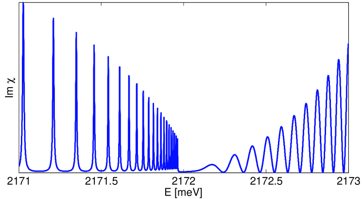
Figure 4: Aborption spectrum in a one-dimensional model, calculated by the formula (48), taking into account the excitonic states with n=2-20.

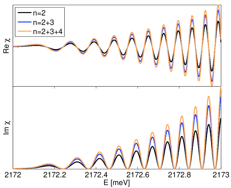
Figure 5: Real and imaginary part of susceptibility in the energetic region above the gap.

VII Optical functions and exciton effect

The complete results will contain the exciton effect, which in our theoretical treatment is related to the resonant denominator $Q$. The results are displayed in Figs. 6-10. In Fig. 6 we illustrate the influence of excitons on the shape of the susceptibility. The impact of exciton manifests in increasing of the absorption; the FK oscillations increase and move towards higher energies while their period and phase remains almost the same. The FK oscillations become more evident when we plot higher derivatives of the susceptibility.

a) b)

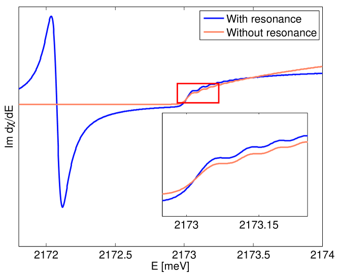
Figure 6: (a) Imaginary part of the susceptibility for a Cu₂O crystal, calculated by Eq. (IV), by taking into account one exciton state and with the applied field strength F=10 V/cm, compared with those calculated without excitonic effects, with parameters as in Fig. 2, (b) The first derivative of susceptibility.

It is shown in Figs. 7-8 where we show the dependence of the second derivative ${\rm d}^{2}\chi/{\rm d}E^{2}$ on the excitation energy. The Fig. 7 shows the imaginary part of susceptibility as a function of energy and field strength. For clarity, the brightness is proportional to the second derivative with respect to the energy. The F-K effect is visible as sinusoidal oscillations with period proportional to the applied field. One can see that the first maximum occurs just above the band gap, at 2172 meV. The thin lines are Stark shifted absorption lines of $P$ and $F$ excitons with principal number up to n=20, calculated according to our method.Zielinska.PRB.2016.b The Fig. 8 shows the full absorption spectrum in a wide range of energy below and over the band gap, highlighting both the F-K effect and excitonic states. One can see that due to the Stark shift, for sufficiently strong field F, the excitonic maxima overlap with the F-K effect. Having the susceptibility, we can calculate the optical functions from the relations (III). According to the discussion presented in Ref.Zielinska.PRB.2016.b the polaritonic effect in Cu₂O can be neglected so optical functions can be applied with the help of the usual formulas for a dielectric slab of thickness; the transmissivity $T$ is given by expression

$$T=\frac{16|n|^{2}}{|(1+n)^{2}|^{2}}\;e^{-\alpha L}=$$

$$=\frac{16\left(n_{1}^{2}+n_{2}^{2}\right)}{\left[\left(1+n_{1}\right)^{2}-n_{2}^{2}\right]^{2}+4n_{2}^{2}\left(1+n_{1}\right)^{2}}\;e^{-\alpha L}.$$ (51)

Here

$$\alpha=2\frac{\hbar\omega}{\hbar c}\hbox{Im}\,n$$ (52)

denotes the absorption coefficient, and $n$ is the complex refraction coefficient $n=\sqrt{\epsilon_{b}+\chi}=n_{1}+in_{2}$. The results obtained from Eq. (VII) are displayed in Figs. 9 and 10. As can be seen from Fig. 9 the transmission spectrum has characteristic FK oscillations in the energy region above the gap. Again as expected, their amplitude and periodicity relay on the electric field strength. This effect is more pronounced in Fig. 10, where the spectrum of transmission difference as the of energy is displayed. The positions of oscillations‘ minima and maxima are in perfect agreement with peaks for excitation energies predicted by formula (31).

VIII Discussion and conclusions

We wish to summarize briefly the results we have obtained by applying the dynamical density matrix approach for the optical properties of semiconductor‘s with Rydberg excitons exposed to a static electric field. We have developed a simple mathematical procedure to calculate electro-optical functions of semiconductor crystal with symmetry where $P$-exciton transitions are dipole allowed. For excitation energies larger than the fundamental gap we observe oscillations in all optical functions which are identified with Franz-Keldysh oscillations. Their periodicity with respect to the excitation energy, the amplitudes and the dependence on the applied field strength was calculated and presented in the form of analytical expressions. The results differ from the known results on FK effect for $S$ excitons. We have also examined the influence of the coherence of the carriers with the electromagnetic field. The presented method has been used to investigate electro-optical functions of Cu₂O crystal for the case of normal incidence and the static electric field applied in the same direction.

Franz-Keldysh effect provides the optoelectronic mechanism to create and control the electro-modulations which might be an essential and flexible tool for constructing optical compatible output devices e.g., a modulator or detectors with an off-chip laser. The copper oxide-based optoelectronic modulators employing Franz-Keldysh effect might show great promise in meeting the strict energy requirements with controlled modification of the reflection/transmission modulation.

The experimental data for FK effect in Cu₂O are not available yet, but we hope that our theoretical considerations might stimulate experiments of the electro-optical properties of this crystal for above gap regime. We conclude that the dynamical density matrix approach is well suited to describe the macroscopic fields (static and dynamic) and the microscopic excitons in all limits of physical interest.

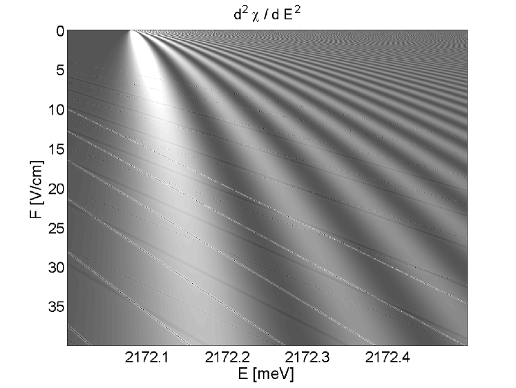
Figure 7: The spectrum of the second derivative of susceptibility for a Cu₂O crystal and the applied field strength $F$=0-40 V/cm. The long period F-K oscillations are superimposed on Stark-shifted excitonic states, seen as thin lines.

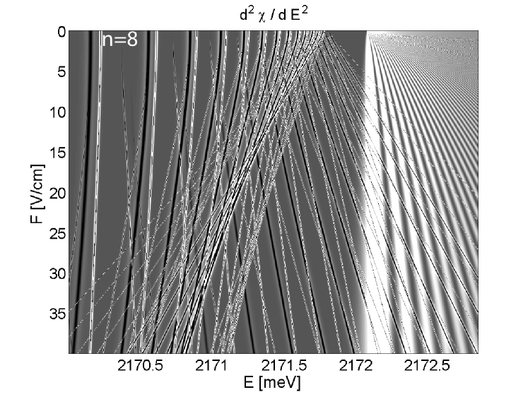
Figure 8: The same as in Fig. 7, over a wider range of energy. The border of F-K oscillations at 2172 meV is readily visible. Excitonic states with $n$=8-20 are taken into account.

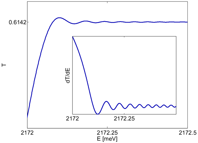
Figure 9: Transmission spectrum for a Cu₂O crystal with thickness 30 $\mu$m, calculated by the formula (VII).

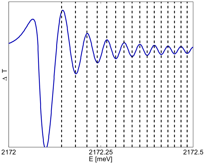
Figure 10: The spectrum of the difference $\Delta T=T(F=10~{}\mbox{V/cm})-T(F=0)$. The dashed lines indicate the position of peaks obtained from the Eq. (31).

References

- (1) Y. Frenkel, On transformation of light into heat in solids, I, Phys. Rev. 37, 17 (1931); On transformation of light into heat in solids, II, Phys. Rev. 37, 1276 (1931).
- (2) R. Peierls, Zur Theorie der Absorptionsspektren fester Körper, Annln. Physk 13, 905 (1932).
- (3) G. H. Wannier, The Structure of Electronic Excitation Levels in Insulating Crystals, Phys. Rev. 52, 191 (1937).
- (4) N. F. Mott, Conduction in polar crystals, II, Trans. Faraday Soc. 34, 500 (1938).
- (5) Gross, E. F., Karryjew, N. A. Dokl. Akad. Nauk SSSR 84, 471�474 (1952).
- (6) R. S. Knox, Theory of Excitons (Academic Press, New York, 1963).
- (7) F. Bassani and G. Pastori-Parravicini, Electronic States and Optical Transitions in Solids (Pergamon Press, Oxford, 1975).
- (8) V. M. Agranovich and V. L. Ginzburg, Crystal Optics with spatial Dispersion and Excitons (Springer Verlag, Berlin, 1984).
- (9) A. Stahl and I. Balslev, Electrodynamics of the Semiconductor Band Edge (Springer-Verlag, Berlin-Heidelberg-New York, 1987).
- (10) G. La Rocca, Wannier-Mott Excitons in Semiconductors. In: Electronic Excitations in Organic Based Nanostructures, ed. by V. M. Agranovich and G. F. Bassani, Thin Films and Nanostructures, vol. 31, Elsevier, Amsterdam, 2003, pp. 97-128.
- (11) F. Bassani, Polaritons. In: Electronic Excitations in Organic Based Nanostructures, ed. by V. M. Agranovich and G. F. Bassani, Thin Films and Nanostructures , Vol. 31, 129-183 (2003) (Elsevier, Amsterdam, 2003, ISBN: 0-12-533031-6).
- (12) V. M. Agranovich, Excitations in Organic Solids (Oxford University Press, Oxford, 2009, ISBN 978 0 19 9234417).
- (13) P. Y. Yu and M. Cardona, Fundamentals of Semiconductors, 4th Ed., (Springer, Berlin-Heidelberg, ISBN 978-3-642-00709-5, 2010).
- (14) C. F. Klingshirn, Semiconductor Optics, 4th ed. (Springer, Berlin Heidelberg, ISBN 978-3-642-28362-8, 2012).
- (15) D. Fröhlich, A. Kulik, B. Uebbing, A. Mysyrowicz, V. Langer, H. Stolz, and W. von der Osten, Coherent Propagation and Quantum Beats of Quadrupole Polaritons in Cu20, Phys. Rev. Lett. 67, 2343 (1991).
- (16) S. Nikitine, Experimental investigations of exciton spectra in ionic crystals, Philisophical Magazine 4, 1 (1959).
- (17) D. Fröhlich and R. Kenklies, Polarization dependence of two-photon magnetoabsorption of the 1s exciton in Cu2O, Phys. Stat. Sol. (b) 111, 247 (1982).
- (18) J. Ghijsen, L. H. Tjeng, J. van Elp, H. Eskes, J. Westerink, G. A. Sawatzky, and M. T. Czyzyk, Electronic structure of Cu2O and CuO, Phys. Rev. B. 38, 11 322 (1988).
- (19) A. Jolk, M. Jörger, and C. Klingshirn, Exciton lifetime, Auger recombination, and exciton transport by calibrated differential absorption spectroscopy in Cu2O, Phys. Rev. B. 65, 245209 (2002).
- (20) M. Jörger, T. Fleck, C. Klingshirn, and R. von Baltz, Midinfrared properties of cuprous oxide: High-order lattice vibrations and intraexcitonic transitions of the 1s paraexciton, Phys. Rev. B. 71, 235210 (2005).
- (21) H. Stolz, R. Schwartz, F. Kieseling, S. Som, M. Kaupsch, S. Sobkowiak, D. Semkat, N. Naka, T. Koch, and H. Fehske, Condensation of excitons in Cu2O at ultracold temperatures: experiment and theory, New Journal of Physics 14, 105007 (2012).
- (22) T. Kazimierczuk, D. Fröhlich, S. Scheel, H. Stolz, and M. Bayer, Giant Rydberg excitons in the copper oxide Cu2O, Nature 514, 344 (2014).
- (23) J. Thewes, J. Heckötter, T. Kazimierczuk, M. Aßmann, D. Fröhlich, M. Bayer, M. A. Semina, and M. M. Glazov, Observation of High Angular Momentum Excitons in Cuprous Oxide, Phys. Rev. Lett. 115, 027402 (2015).
- (24) S. Zielińska-Raczyńska, G. Czajkowski, and D. Ziemkiewicz, Optical properties of Rydberg excitons and polaritons, Phys. Rev. B 93, 075206 (2016).
- (25) F. Schöne, S.-O. Krüger, P. Grünwald, H. Stolz, M. Aßmann, J. Heckötter, J. Thewes, D. Fröhlich, and M. Bayer, Deviations of the exciton level spectrum in Cu2O from the hydrogen series, Phys. Rev. B 93, 075203 (2016).
- (26) F. Schweiner, J. Main, and G. Wunner, Linewidths in excitonic absorption spectra of cuprous oxide, Phys. Rev. B 93, 085203 (2016).
- (27) P. Grünwald, M. Aßmann, J. Heckötter, D. Fröhlich, M. Bayer, H. Stolz, and S. Scheel, Signatures of Quantum Coherences in Rydberg Excitons, Phys. Rev. Lett. 117, 133003 (2016).
- (28) J. Heckötter, M. Freitag, D. Fröhlich, M. Aßmann, M. Bayer, M. A. Semina, and M. M. Glazov, Scaling laws of Rydberg excitons, Phys. Rev. B 96, 125142 (2017).
- (29) F. Schweiner, J. Main, G. Wunner, and Ch. Uihlein, Even exciton series in Cu2O, Phys. Rev. B 95, 195201 (2017).
- (30) F. Schweiner, J. Ertl, J. Main, G. Wunner, and Ch. Uihlein, Exciton-polaritons in cuprous oxide: Theory and comparison with experiment, Phys. Rev. B 96, 245202 (2017).
- (31) V. Walther, R. Johne, and T. Pohl, Giant optical nonlinearities from Rydberg-excitons in semiconductor microcavities, threearXiv: 1711.01601v1 [cond-mat.quant-gas] 5 Nov 2017.
- (32) S. Zielińska-Raczyńska, D. Ziemkiewicz, and G. Czajkowski, Electrooptical properties of Rydberg excitons, Phys. Rev. B 94, 045205 (2016).
- (33) F. Schweiner, J. Main, G. Wunner, M. Freitag, J. Heckötter, Ch. Uihlein, M. Aßmann, D. Fröhlich, and M. Bayer, Magnetoexcitons in cuprous oxide, Phys. Rev. B 95, 035202 (2017).
- (34) S. Zielińska-Raczyńska, D. Ziemkiewicz, and G. Czajkowski, Magneto-optical properties of Rydberg excitons: Center-of-mass quantization approach, Phys. Rev. B 95, 075204 (2017).
- (35) M. Aßmann, J. Thewes, and M. Bayer, Quantum chaos and breaking of all antiunitary symmetries in Rydberg excitons, Nature Materials 15, 741 (2016).
- (36) F. Schweiner, P. Rommel, J. Main, and G. Wunner, Exciton-phonon interaction breaking all antiunitary symmetries in external magnetic fields, Phys. Rev. B 96, 035207 (2017).
- (37) F. Schweiner, J. Main, and G. Wunner, Magnetoexcitons Break Antiunitary Symmetries, Phys. Rev. Lett. 118, 046401 (2017).
- (38) T. Kitamura, M. Takahata1, and N. Naka, Quantum number dependence of the photoluminescence broadening of excitonic Rydberg states in cuprous oxide, J. Luminescence 192, 808 (2017).
- (39) J. Heckötter, M. Freitag, D. Fröhlich, M. Aßmann, M. Bayer, P. Grünwald, F. Schöne, D. Semkat, H. Stolz, and S. Scheel, Rydberg excitons in the presence of an ultralow-density electron-hole plasma, arXiv: 1709.00891v1 [cond-mat.mtrl-sci] 4 Sep 2017.
- (40) W. Franz, Einfluß eines elektrischen Feldes auf eine optische Absorptionskante, Z. Naturforschung 13a, 484 (1958).
- (41) L. V. Keldysh, Behaviour of Non-Metallic Crystals in Strong Electric Fields,Zhurn. Eksp. Teoret. Fiz. 34,1138 (1958); (English trans.: Sov. Phys. JETP 7, 788 (1958)).
- (42) K. Tharmalingam Optical Absorption in the Presence of a Uniform Field, Phys. Rev. 130, 2204 (1963).
- (43) K. S. Viswanathan and J. Callaway, Dielectric Constant of a Semiconductor in an External Electric Field, Phys. Rev. 143, 564 (1966).
- (44) D. A. Aspnes, Electric-Field Effects on Optical Absorption near Thresholds in Solids, Phys. Rev. 147, 554 (1966).
- (45) F. Aymerich and F. Bassani, Electric-field effects on interband transitions, Il Nuovo Cimento 48 B, 358 (1967).
- (46) H. I. Ralph, On the theory of Franz-Keldysh effect, J. Phys. C 1, 378 (1968).
- (47) M. Cardona, Modulation Spectroscopy, Suppl.11 of Solid State Physics, ed. by F. Seitz, D. Turnbull, and H. Ehrenreich, (Academic Press, New York-London 1969).
- (48) D. F. Blossey, Wannier Exciton in an Electric Field. I. Optical Absorption by Bound and Continuum States, Phys. Rev. B 2, 3976 (1970).
- (49) D. F. Blossey, Wannier Exciton in an Electric Field. II. Electroabsorption in Direct-Band-Gap Solids, Phys. Rev. B 3, 1382 (1971).
- (50) F. L. Lederman and J. D. Dow, Theory of electroabsorption by anisotropic and layered semiconductors. I. Two-dimensional excitons in a uniform electric field, Phys. Rev. B 13, 1633 (1976).
- (51) A. G. Aronov and A. S. Ioselevich, Exciton Electrooptics. In: Excitons, ed. by E. I. Rashba and M. D. Sturge (North Holland, Amsterdam 1982).
- (52) H. Schneider, A. Fischer, and K. Ploog, Franz-Keldysh oscillations and Wannier-Stark localization in GaAs/AlAs superlattices with single-monolayer AlAs barriers, Phys. Rev. B 45, 6329 (1992).
- (53) B. Schlichterle, G. Weiser, M. Klenk, F.Mollot, and Ch.Starck, Effective masses in In1-xGax As superlattices derived from Franz-Keldysh oscillations, Phys. Rev. B 52, 9003 (1995).
- (54) M. Nakayama, T. Nakanishi, K. Okajima, M. Ando and H. Nishimura, Miniband structures and effective masses of GaAs/AlAs superlattices with ultra-thin layers, Solid State Comm. 102, 803 (1997).
- (55) H. Shen and M. Dutta, Franz-Keldysh oscillations in modulation spectroscopy, J. Appl. Phys. 78, 2151 (1995); doi: 10.1063/1.360131.
- (56) G. Czajkowski, M. Dressler, and F. Bassani, Electro-optical properties of semiconductor superlattices in the regime of Franz-Keldysh oscillations, Phys. Rev. B 55, 5243 (1997).
- (57) G. Czajkowski and L. Silvestri, Electric and magnetic field effects on optical properties of excitons in semiconductor nanostructures. In: Electrons and photons in solids - A volume in honour of Franco Bassani, edited by G. Grosso, G. C. La Rocca and M. Tosi (Scuola Normale Superiore - Pubblicazioni della classe di scienze, Pisa, Italy, 2001), pp. 271-288.
- (58) G. Czajkowski, F. Bassani, and L. Silvestri, Excitonic Optical Properties of Nanostructures: Real Density Matrix Approach, Rivista del Nuovo Cimento 26, 1-150 (2003).
- (59) M. Dressler, F. Bassani, and G. Czajkowski, Electro-optical properties of excitons in polydiacetylene chains, Eur. Phys. J. B 10, 681 (1999).
- (60) J. R. Madureira, M. Z. Maialle, M. H. Degani, Franz-Keldysh Effect in Semiconductor T-Wire in Applied Magnetic Field, Brazilian Journ. Phys. 34, 663 (2004).
- (61) R. K. Schaevitz, D. S. Ly-Gagnon, J. E. Roth, E. H. Edwards, and D. A. B. Miller, Indirect absorption in germanium quantum wells, AIP Advances 1, 032164 (2011).
- (62) S. J. Lee, Ch. W. Sohn, H.-J. Jo, I. S. Han, J. S. Kim, S. K. Noh, H. Choi, J.-Y. Leem, Temperature Dependence of the Photovoltage from Franz-Keldysh Oscillations in a GaAs p+-i-n+ Structure, J. Korean Phys. Society 67, 916, (2015).
- (63) Patent US 5365334 A, Micro photoreflectance semiconductor wafer analyzer; Photoreflectance spectral analysis of semiconductor laser structures US 6195166 B1; Optical measuring method for semiconductor multiple layer structures and apparatus therefor US 7038768 B2.
- (64) Handbook of Mathematical Functions, edited by M. Abramowitz and I. Stegun (Dover Publications, New York 1965).
- (65) E. T. Whittaker and G. N. Watson, A Course of Modern Analysis (Cambridge Un. Press, Cambridge, 1935, Reissued in the Cambridhe Math. Library Series, 1996, ISBN 05215880703).
- (66) I. S. Gradshteyn and I. M. Ryzhik, Table of Integrals, Series, and Products, edited by A. Jeffrey and D. Zwillinger, 7th Edition (Academic Press, Elsevier, Amsterdam, 2007, ISBN-13:978-0-12-373637-6).
- (67) O. Vallée and M. Soares, Airy Functions and Applications to Physics (Imperial College Press, London, 2004, ISBN: 1-86094-478-7).