Constraints On Short, Hard Gamma-Ray Burst Beaming Angles From Gravitational Wave Observations

Abstract

The first detection of a binary neutron star merger, GW170817, and an associated short gamma-ray burst confirmed that neutron star mergers are responsible for at least some of these bursts. The prompt gamma ray emission from these events is thought to be highly relativistically beamed. We present a method for inferring limits on the extent of this beaming by comparing the number of short gamma-ray bursts observed electromagnetically to the number of neutron star binary mergers detected in gravitational waves. We demonstrate that an observing run comparable to the expected Advanced LIGO 2016–2017 run would be capable of placing limits on the beaming angle of approximately $\theta\in(2.88^{\circ},14.15^{\circ})$, given one binary neutron star detection. We anticipate that after a year of observations with Advanced LIGO at design sensitivity in 2020 these constraints would improve to $\theta\in(8.10^{\circ},14.95^{\circ})$.

1 Introduction

Gamma-ray bursts (GRBs) are extremely energetic cosmological events observed approximately once per day. There appear to be at least two separate populations of gamma-ray bursts, divided roughly according to their duration and spectral hardness Kouveliotou et al. (1993), although with significant overlap obscuring any clear distinction between populations Zhang et al. (2009); Bromberg et al. (2013). Those with long durations ($\gtrsim 2\,\mathrm{s}$) and softer spectra are associated with core collapse supernovae Galama et al. (1998); MacFadyen & Woosley (1999); Woosley & Bloom (2006). Short, hard GRBs (SGRBs) were long suspected of being the signatures of compact binary coalescences involving at least one neutron star (NS) Blinnikov et al. (1984); Eichler et al. (1989); Paczyński (1991); Narayan et al. (1992); Lee & Ramirez-Ruiz (2007). Both NS–NS and NS– black hole (BH) progenitors are possible, with the requirement that a post merger torus of material accretes onto a compact central object Blandford & Znajek (1977); Rosswog & Ramirez-Ruiz (2002); Giacomazzo et al. (2013).

The first observation of a NS–NS coalescence event, GW170817 Abbott et al. (2017a), its association with GRB 170817A Abbott et al. (2017b); Goldstein et al. (2017); Savchenko et al. (2017) and, later, multi-wavelength electromagnetic emission, including a kilonova Abbott et al. (2017), confirmed that compact binary mergers are the engines of at least some short gamma-ray bursts. The gravitational wave (GW) observation placed only weak constraints on the viewing angle due to a degeneracy between distance and inclination of the binary to the line of sight Abbott et al. (2017a). However, GRB 170817A was not typical of SGRBs, being around $10^{4}$ times less energetic Goldstein et al. (2017). This, in addition to other aspects of the electromagnetic emission, has been widely interpreted as indicating that GRB 170817A was not viewed from within the cone of a canonical jet with a top-hat profile (see e.g. Fong et al. (2017); Kasliwal et al. (2017); Gottlieb et al. (2017); Haggard et al. (2017)).

A population of GW–SGRB observations could also allow us to measure the fraction of SGRBs associated with each progenitor type, and associated redshifts will enable a relatively systematics-free measurement of the Hubble parameter at low redshift, which would provide constraints on cosmological models Schutz (1986); Nissanke et al. (2010); Chen & Holz (2013); Abbott et al. (2017).

In this work we consider a population of binary merger sources, with and without SGRB counterparts, assuming that the vast majority of these counterparts would be viewed from within the cone of a standard jet. This is motivated by the fact that most mergers would be expected to occur at distances much greater than GW170817 and that weak, off-axis gamma ray emission would in all likelihood go undetected. With such a population we can constrain the average opening angle Chen & Holz (2013); Clark et al. (2015); Abbott et al. (2016a).

We investigate what statements can currently be made on the beaming angle itself using the bounds placed on the binary merger rate ${{\mathcal{R}}}$ from all-sky, all-time GW searches and explore the potential for direct inference of SGRB beaming angles in the advanced detector era. We first discuss the relationship between SGRBs and compact binary coalescences. In particular, we will focus on NS–NS inspirals as the progenitors of SGRBs. We then present our method for robustly inferring the jet opening angles using only GW observations. We demonstrate our method assuming the nominal number of GW signals observed from NS–NS inspirals expected for Advanced LIGO (aLIGO) and Advanced Virgo in planned observing scenarios, as defined in Abbott et al. (2013). Finally, we conclude with a discussion on the implications of our work as well as possible avenues for further extension of the work presented here.

2 Short gamma-ray bursts and compact binary coalescences

At their design sensitivities, the current generation of advanced GW detectors could observe NS–NS mergers out to distances of ${\sim}400\,\mathrm{Mpc}$ at a rate of $0.1\text{--}200\,$yr^-1 Abbott et al. (2013). It is worth noting that at galactic or near-galactic distances, soft gamma-ray repeater (SGR) hyperflares can resemble SGRBs. These SGR hyperflares are the likely explanations for GRB 070201 and GRB 051103, since compact binary coalescences at the distance of their probable host galaxies were excluded with greater than $90\%$ confidence Abbott et al. (2008); Abadie et al. (2012a).

Given the link between SGRBs and compact binary coalescences, it is interesting to ask whether the SGRB beaming angle can be inferred from GW observations. As discussed in Clark et al. (2015), a comparison of the populations of observed SGRBs and NS–NS mergers may be the most promising avenue for this. Motivated by the study in Chen & Holz (2013), we note that if the SGRB population posseses a distribution of beaming angles then the observed rate of SGRBs is related to the rate of NS–NS coalescences ${{\mathcal{R}}}$ via,

$${{\mathcal{R}}_{\mathrm{grb}}}=\epsilon{{\mathcal{R}}}\left\langle 1-\cos\theta\right\rangle,$$ (1)

where angled brackets $\langle\rangle$ indicate the population mean and $\epsilon$ is the probability that a binary coalescence results in an observed SGRB. In this work, we assume an illustrative ${{\mathcal{R}}_{\mathrm{grb}}}=10$ Gpc^-3 yr^-1 Nakar (2007); Dietz (2011) and we shall refer to $\epsilon$ as the SGRB efficiency. The method we present, however, is amenable to using alternative values for ${{\mathcal{R}}_{\mathrm{grb}}}$, or indeed to being extended to sampling values from a prior distribution on the SGRB rate. Generally, the efficiency with which NS–NS mergers produce SGRBs is unknown but will depend on a variety of progenitor physics. In particular, a significant fraction of NS–BH systems may be incapable of powering an SGRB Pannarale & Ohme (2014). Combining this knowledge with measurements of the binary parameters of of a population of GW–SGRB observations could be used to constrain $\epsilon$. In this work, we will make no attempt to characterise $\epsilon$ and we simply aim to provide a framework which allows one to incorporate various levels of assumptions (or ignorance) regarding its value.

If the SGRB population has a distribution of beaming angles, as would seem likely from electromagnetic (EM) observations Fong et al. (2015), characterising the relative rates of SGRB and NS–NS coalescence will inform us as to the mean of that population, $\langle\theta\rangle$. To explore this point further we construct a simple Monte Carlo simulation to study the effect on the relative rates of SGRBs and NS–NS mergers. We arrange the following toy problem:

1. Set the number of ‘observed’ SGRBs to zero: $N_{\mathrm{GRB}}=0$.

2. Draw $N_{\mathrm{{\small\acs{NS}-\acs{NS}}}}$ values of orbital inclination $\iota$ from a distribution which is uniform in $\cos\iota$ in the range $[0,1]$.

3. For each value of $\iota$, draw a value for the beaming angle $\theta$, from some distribution with finite width and limited to the range $(0,90]^{\circ}$.

4. If $\iota<\theta$ then this combination of orbital inclination and beaming angle would result in an observable SGRB, so increment $N_{\mathrm{GRB}}$.

Such a simulation allows us to study the ratio of the number of observed SGRB to the total number of NS–NS mergers $N_{\mathrm{GRB}}/N_{\mathrm{{\small\acs{NS}-\acs{NS}}}}$. Since it is the comparison of the rates of these events that informs our inference on $\theta$, studying the ratio $N_{\mathrm{GRB}}/N_{\mathrm{{\small\acs{NS}-\acs{NS}}}}$ provides some intuition as to the effect and features of various $\theta$ distributions. Figure 1 plots this ratio as a function of various truncated normal distributions to demonstrate the effect of shifting the mean and scaling the width of the distribution. Points along the $x$-axis correspond to different choices of the distribution width $\sigma_{\theta}$, and the separate curves correspond to different choices of the distribution mean $\langle\theta\rangle$. Let us denote this truncated normal distribution ${\mathcal{N}}(\langle\theta\rangle,\sigma_{\theta})$. We stress here that such $\theta$ distributions are not intended to represent the true distribution; they are merely intended to easily demonstrate the qualitative effects of different $\theta$ distributions on the ratio $N_{\mathrm{GRB}}/N_{\mathrm{{\small\acs{NS}-\acs{NS}}}}$.

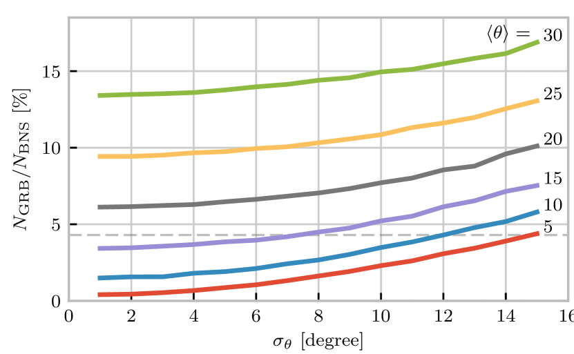
Figure 1: Expected relative numbers of observed GRBs and binary coalescences for different distributions on the GRB beaming angle. Lines in the figure correspond to jet angle population means, while the $x$-axis shows the width of the distribution. All distributions are Gaussian, truncated at $(0,90]$ degrees.

Figure 1 reveals that a population of SGRB beaming angles with a large mean but narrow width is, on the basis of rate measurements, indistinguishable from a population of SGRB beaming angles with a small mean and large width. For example, for the ${\mathcal{N}}(15,9)$ and ${\mathcal{N}}(10,13)$ beaming angle populations, the ratios of $N_{\mathrm{GRB}}/N_{\mathrm{{\small\acs{NS}-\acs{NS}}}}$ are almost equal ($\sim 4.8\%$). Thus, a sufficiently wide spread of SGRB beaming angles will yield relatively high rates for NS–NS and SGRBs that could lead to an overestimate of the mean beaming angle. The population-based constraints on $\theta$ must, therefore, be regarded as upper bounds on the mean of a distribution of beaming angles. Having said this, for a given mean value $\langle\theta\rangle$, the ratio is rather insensitive to the width.

3 From Rates To Beaming Angles

In this section, we discuss our approach to estimating the SGRB beaming angle based on the binary neutron star inspiral rate, estimated through a number of GW observations of NS–NS coalescence. We demonstrate the approach by considering plausible detection scenarios for aLIGO Abbott et al. (2013). Our ultimate goal is to develop a generic approach that folds in uncertainties in the NS–NS merger rate and our ignorance about the probability with which such mergers actually result in SGRBs. An overview of the general method is as follows:

1. Estimate the posterior probability distribution on the NS–NS merger rate in the local universe from a number of observed gravitational wave signals and our knowledge of the sensitivity of the detectors. We construct a joint posterior distribution on the NS–NS rate and the (unknown) probability $\epsilon$ that a given merger results in a SGRB.

2. Use equation 1, which relates the NS–NS merger and SGRB rates via the geometry of the beaming angle, to transform the rate posterior probability to a posterior probability on the mean SGRB beaming angle.

3. Marginalize over $\epsilon$. We choose to consider $\epsilon$ a nuisance parameter because, to date, there is no accurate estimate of this parameter and it is not the main focus of our analysis.

3.1 Constructing The Rate Posterior

Our goal is to infer the posterior probability distribution for the mean SGRB beaming angle $\theta$ from GW constraints on the rate of NS–NS coalescence ${{\mathcal{R}}}$. The core ingredient to the analysis is the posterior probability distribution on the coalescence rate $p({{\mathcal{R}}}|D,I)$, where $D$ represents some GW observation and $I$ denotes other unenumerated prior information. We will first demonstrate how $p({{\mathcal{R}}}|D,I)$ may be constructed for a few projected observing scenarios from Abbott et al. (2013). Later, in section 5, we will extend the analysis to place limits on $\theta$ based upon the lack of detection during O1. Previously, a comparison of rates was used to place a lower limit on the beaming angle in Abbott et al. (2016a).

To form the posterior on the coalescence rate, we begin by constructing the posterior on the signal rate. Note that these are not identical since only those NS–NS mergers which occur within a certain range yield a detectable signal. GW data analysis pipelines (e.g. FINDCHIRP Allen et al. (2012), PyCBC Dal Canton et al. (2014); Usman et al. (2016); Nitz et al. (2017)) identify discrete ‘candidate events’ which are characterised by network signal-to-noise ratios, $\rho_{c}$, which, for the case of NS–NS searches, indicate the similarity between the detector data and a set of template NS–NS coalescence waveforms. The measured rate $r$ of these events consists of two components: a population of true GW signals, $s$; and a background rate, $b$, due to noise fluctuations due to instrumental and environmental disturbances.

$$r=s+b\begin{cases}s=\text{signal rate}\\ b=\text{background rate}.\end{cases}$$ (2)

Typically for an all-sky, all-time analysis, like that described in Usman et al. (2016), the significance of a candidate event is empirically measured against ‘background’ data representative of the detector noise, which naturally varies from candidate to candidate. A detection requires this significance to be above some pre-determined threshold (e.g. $5\sigma$ for GW150914 and GW151226 Abbott et al. (2016b, c)). We follow the method in Abbott et al. (2013), which defines a detection as a candidate with $\rho_{c}\geq 12$, corresponding approximately to $b=10^{-2}$ yr^-1. Since the background rate $b$ is known, we are just left with the problem of inferring the signal rate $s$. Assuming a uniform prior on $s$ and a Poisson process underlying the events, it may be shown (e.g., Gregory (2010)) that the posterior for the signal rate, given a known background rate $b$ and $n$ events observed over a time period $T$ is,

$$p(s|n,b,I)=C\frac{T\left[(s+b)T\right]^{n}e^{-(s+b)T}}{n!},$$ (3)

where,

$$C^{-1} = \frac{e^{-bT}}{n!}\int_{0}^{\infty}{\mathrm{d}}(sT)(s+b)^{n}T^{n}e^{-sT}$$ (4)

$$= \sum_{i=0}^{n}\frac{(bT)^{i}e^{-bT}}{i!}.$$ (5)

Finally, we can transform the posterior on the signal rate to the underlying coalescence rate via our knowledge of the sensitivity of the GW analysis. In particular, the signal detection rate is simply the product of the intrinsic coalescence rate ${{\mathcal{R}}}$ and the number of NS–NS mergers which would result in a GW signal with $\rho_{c}\geq 12$. Expressing the binary coalescence rate in terms of the number of mergers per Milky Way Equivalent Galaxy (MWEG), per year then we require the number of galaxies $N_{\mathrm{G}}$ which may be probed by the GW analysis. At large distances, this is well approximated by LIGO Scientific Collaboration & Virgo Collaboration (2010),

$$N_{G}=\frac{4}{3}\pi\left(\frac{{\mathcal{D}}_{\mathrm{hor}}}{\mathrm{Mpc}}\right)^{3}(2.26)^{-3}(0.0116),$$ (6)

where ${\mathcal{D}}_{\mathrm{hor}}$ is the horizon distance (defined as the distance at which an optimally-oriented NS–NS merger yields $\rho_{c}\geq 12$), the factor of 2.26 results from averaging over sky-locations and orientations, and $1.16\times 10^{-2}$ Mpc^-3 is the extrapolated density of MWEG in space.

Finally, the posterior on the binary coalescence rate ${{\mathcal{R}}}$ is obtained from a trivial transformation of the posterior on the signal rate $s$,

$$p({{\mathcal{R}}}|n,T,b,{\mathcal{D}}_{\mathrm{hor}}) = p(s|n,T,b)\left|\frac{{\mathrm{d}}s}{{\mathrm{d}}{{\mathcal{R}}}}\right|$$ (7)

$$= N_{G}({\mathcal{D}}_{\mathrm{hor}})p(s|n,T,b).$$ (8)

We see that in this approach, the rate posterior depends only on the number of signal detections $n$, the observation time $T$, the background rate $b$, and the horizon distance of the search ${\mathcal{D}}_{\mathrm{hor}}$. It is precisely these quantities that comprise the detection scenarios outlined in Abbott et al. (2013). Before constructing expected rate posteriors, we outline the transformation from rate to beaming angle.

3.2 Constructing the beaming angle posterior

Inferences of the SGRB beaming angle are made from the posterior probability density on the beaming angle $p(\theta|D,I)$ where, as usual, $D$ indicates some set of observations and $I$ unenumerated prior knowledge. Our goal is to transform the measured posterior probability density on the rate ${{\mathcal{R}}}$ to a posterior on the beaming angle. First, note that we can express the joint distribution $p(\theta,\epsilon|D,I)$ as a Jacobian transformation of the joint distribution $p({{\mathcal{R}}},\epsilon|D,I)$:

$$p(\theta,\epsilon)=p({{\mathcal{R}}},\epsilon)\left\lvert\left\lvert\frac{\partial({{\mathcal{R}}},\epsilon)}{\partial(\theta,\epsilon)}\right\rvert\right\rvert,$$ (9)

where we have dropped conditioning statements for notational convenience. The Jacobian determinant can be computed from equation 1. It is then straightforward to marginalize over $\epsilon$ to yield the posterior on $\theta$ itself:

$$p(\theta) = \int_{\epsilon}p(\theta,\epsilon)~{}{\mathrm{d}}\epsilon$$ (10)

$$= \int_{\epsilon}p({{\mathcal{R}}},\epsilon)\left\lvert\left\lvert\frac{\partial({{\mathcal{R}}},\epsilon)}{\partial(\theta,\epsilon)}\right\rvert\right\rvert~{}{\mathrm{d}}\epsilon$$ (11)

$$= \frac{2{{\mathcal{R}}_{\mathrm{grb}}}\sin\theta~{}p({{\mathcal{R}}})}{(\cos\theta-1)^{2}}\int_{\epsilon}\frac{p(\epsilon)}{\epsilon}~{}{\mathrm{d}}\epsilon,$$ (12)

where we have assumed $\epsilon$ and ${{\mathcal{R}}}$ are logically independent such that,

$$p(\epsilon,{{\mathcal{R}}})=p(\epsilon|{{\mathcal{R}}})p({{\mathcal{R}}})=p(\epsilon)p({{\mathcal{R}}}).$$ (13)

It is important to note that the entire procedure of deriving the jet angle posterior is completely independent of the approach used to derive the rate posterior. In the preceding section we adopted a straightforward Bayesian analysis of a Poisson rate which is amenable to a simple application of plausible future detection scenarios; there is no inherent requirement to use that method to derive the rate posterior.

Given the posterior on the rate, $p({{\mathcal{R}}})$, the final ingredient in this approach is the specification of some prior distribution for $\epsilon$. Given the lack of information on the value and distribution of $\epsilon$, we choose three plausible priors and study their effects on our beaming angle inference. Our choice of priors are:

Delta-function

$p(\epsilon)=\delta(\epsilon=0.5)$; the probability that NS–NS mergers yield SGRBs is known to be 50% exactly.

Uniform

$p(\epsilon)=U(0,1)$; the probability that NS–NS mergers yield SGRBs may lie anywhere $\epsilon\in(0,1]$ with equal support in that range.

Jeffreys

$p(\epsilon)=\beta(\frac{1}{2},\frac{1}{2})$; treating the outcome of a NS–NS merger as a Bernoulli trial in which a SGRB constitutes ‘success’ and $\epsilon$ is the probability of that success, the least informative prior, as derived from the square root of the determinant of the Fisher information for the Bernoulli distribution, is a $\beta$-distribution with shape parameters $\alpha=\beta=\frac{1}{2}$.

4 Prospects For Beaming Angle Constraints With Advanced LIGO

We now demonstrate the derivation of the rate posterior $p({{\mathcal{R}}})$ and the subsequent transformation to the beaming angle posterior $p(\theta)$. We consider four GW observation scenarios with aLIGO based on the work in Abbott et al. (2013). An observing scenario essentially consists of an epoch of aLIGO operation, which defines an expected search sensitivity (i.e., NS–NS horizon distance ${\mathcal{D}}_{\mathrm{hor}}$) and observation time $T$; as well as an assumption on the rate of NS–NS coalescence in the local universe ${{\mathcal{R}}}$. Each observing scenario ultimately results in an expectation for the number of observed GWs from NS–NS coalescences. For this study, we assume the ‘realistic rate’ for ${{\mathcal{R}}}$ as described in LIGO Scientific Collaboration & Virgo Collaboration (2010).

Our first goal is to establish the expected number of detections in each scenario. Given the observation time and horizon distance of the observation epoch we first compute the 4-volume accessible to the analysis,

$$V_{\mathrm{search}}=\frac{4}{3}\pi\left(\frac{{\mathcal{D}}_{\mathrm{hor}}}{2.26}\right)^{3}\times\gamma T,$$ (14)

where the factor 2.26 arises from averaging over source sky location and orientation, $T$ is the observation time and $\gamma$ is the duty cycle for the science run. Following Abbott et al. (2013), we take $\gamma=0.5$. For comparison, during the first observing run of aLIGO, the two interferometers observed in coincidence achieving $\gamma_{\mathrm{coinc}}=0.41$. Where there is a range in the horizon distances quoted in Abbott et al. (2013) to account for uncertainty in the sensitivity of the early configuration of the detectors, we use the arithmetic mean of the lower and upper bounds when computing the search volume. Table 1 lists the details of each observing scenario.

Epoch	$T$	${\mathcal{D}}_{\mathrm{insp}}$	$V_{\mathrm{search}}$	Est. NS–NS
	[yr]	[Mpc]	[$\!\times\!10^{6}\mathrm{Mpc}\textthreesuperior\,\mathrm{yr}^{-1}$]	Detections
2015–2016	0.25	40–80	0.05–0.4	0.0005–4
2016–2017	0.5	80–120	0.6–2.0	0.006-20
2018–2019	0.75	120–170	3–10	0.04–100
2020+	1	200	20	0.2–200
2024+	1	200	40	0.4–400

Table 1: Advanced detector era observing scenarios considered in this work. $T$ is the expected duration of the science run and ${\mathcal{D}}_{\mathrm{insp}}$ is the NS–NS inspiral distance for the sensitivity expected to be achieved at the given epoch, which is equal to ${\mathcal{D}}_{\mathrm{hor}}/2.26$. $V_{\mathrm{search}}$ is the sensitive volume of the search, defined by equation 14; the final column contains the estimated range of the number of GW detections. Note that the quoted search volume accounts for a network duty cycle of $\sim 80\%$ per detector. These scenarios are derived from those detailed in Abbott et al. (2013). While the 2020+ and 2024+ scenarios appear identical in terms of the sensitivity of the detectors, the 2024+ scenario includes a third advanced LIGO detector in India. This expansion of the network is expected to lead to an increase in the network duty cycle, and an increase in the area of the sky which the network is sensitive to, resulting in a greater volume being searched per year.

4.1 Posterior Results

Figure 2 shows the NS–NS rate posteriors resulting from the observations in the scenarios in table 1 generated using the procedure described in section 3.1. Where a range of potential inspiral distances is given for a scenario we choose the median value, so for the 2015–2016 scenario we take ${\mathcal{D}}_{\mathrm{insp}}$ to be $60\,\mathrm{Mpc}$, for example. Likewise we choose an illustrative value of $n$, the number of expected GW detections, from each range; these are listed in table 2.

We now use these posteriors together with the prior distributions described in section 3.1 and the observed rate of SGRBs (as described in section 2, we use ${{\mathcal{R}}_{\mathrm{grb}}}=10$ Gpc^-3yr^-1 Nakar (2007); Dietz (2011)) to derive the corresponding beaming angle posteriors.

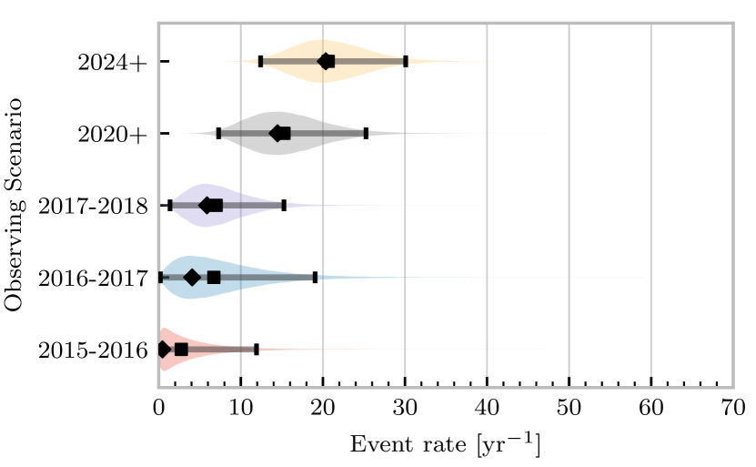
Figure 2: Posterior probability distribution for the rate of NS–NS coalescence assuming the scenarios in table 1. The 95% credible interval is represented with a horizontal line through the centre of the plot, with vertical lines delineating the lower and upper limits; the median is represented by a square marker, and the maximum a posteriori (MAP) value is denoted by a diamond. A summary of these values is given in table 2.

Scenario	$n$	Lower	MAP	Median	Upper
		[$\mathrm{yr}^{-1}$]	[$\mathrm{yr}^{-1}$]	[$\mathrm{yr}^{-1}$]	[$\mathrm{yr}^{-1}$]
2015–2016	0	0.00	0.45	2.80	11.98
2016–2017	1	0.17	4.07	6.74	19.13
2017 – 2018	3	1.37	5.88	6.99	15.26
2020+	10	7.30	14.47	15.25	25.25
2024+	20	12.42	20.35	20.65	30.09

Table 2: Summary of the NS–NS rate posteriors for each of the observing scenarios which are considered in this work; these posteriors are plotted in figure 2. Here $n$ is the number of GW events which were assumed to be observed in each scenario, chosen from the ranges in table 1.

4.1.1 Validation

Before we derive beaming angle posteriors corresponding to the aforementioned observing scenarios, it is useful to establish some form of validation for our procedure. This validation is performed by first selecting values of the beaming angle, the SGRB efficiency, and the rate of NS–NS coalescence. We choose $\theta=10^{\circ}$, and the ‘realistic’ NS–NS rate ${{\mathcal{R}}}=10^{-6}$ Mpc^-3yr^-1. We then compute the value of the SGRB rate that would correspond to these parameter choices. Finally, we simply use this artificial value for ${{\mathcal{R}}_{\mathrm{grb}}}$ in equation 10 when we compute the posterior on the beaming angle, with the understanding that the resulting posterior should yield an inference consistent with the ‘true’ value $\theta=10^{\circ}$.

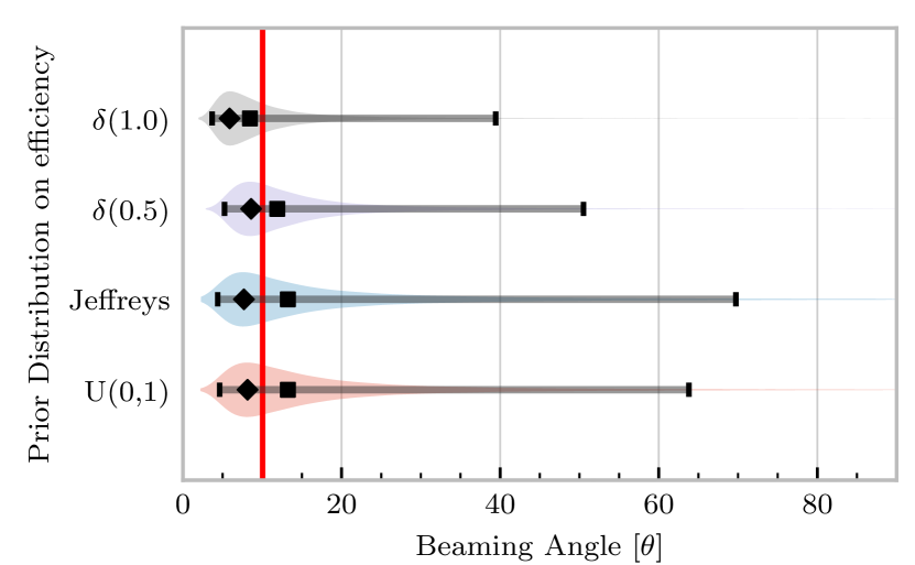
Figure 3: In order to validate the algorithm an artificial scenario was constructed with a known beaming angle by artificially setting a GRB rate of $36.7\,\mathrm{yr}^{-1}$ to induce a beaming angle of $\theta\approx 10^{\circ}$. The algorithm was then tested with the various priors used in the analysis, using the same horizon distance, observing time, and duty cycle as the 2015–2016 observing scenario. to ensure that the correct beaming angle was inferred. These posteriors are based on the simulated 2015–2016 observing scenario (see table 1).

Prior	Lower	MAP	Median	Upper
	[∘]	[∘]	[∘]	[∘]
$\delta(1.0)$	3.68	5.88	8.45	39.44
$\delta(0.5)$	5.24	8.59	11.89	50.51
Jeffreys	4.38	7.69	13.23	69.74
U(0,1)	4.62	8.14	13.23	63.81

Table 3: Summary of the beaming angle posteriors from figure 3, for the 2015–2016 observing scenario, with an artificial GRB rate imposed to produce a target beaming angle of $\theta=10^{\circ}$.

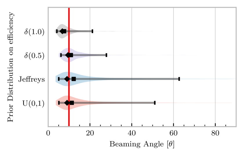
Figure 4: The procedure used to produce figure 3 was repeated for the observing time and the horizon distance of the 2016–2017 observing scenario, with a GRB rate of $28.0\,\mathrm{yr}^{-1}$ used to induce a beaming angle of $\theta\approx 10^{\circ}$.

Prior	Lower	MAP	Median	Upper
	[∘]	[∘]	[∘]	[∘]
$\delta(1.0)$	4.15	6.78	7.62	21.17
$\delta(0.5)$	6.11	9.50	10.88	27.88
Jeffreys	5.05	9.05	12.21	62.72
U(0,1)	5.12	9.05	11.29	51.04

Table 4: Summary of the beaming angle posteriors from figure 4, for the 2016–2017 observing scenario, with an artificial GRB rate imposed to produce a target beaming angle of $\theta\approx 10^{\circ}$.

Figures 3 and 4 show the beaming angle posteriors which result from this analysis for the 2015–2016 and 2016–2017 scenarios respectively for each choice of prior distribution on the efficiency parameter. Unsurprisingly, the most accurate constraints arise when we already have the tightest possible constraints on the SGRB efficiency, $\epsilon$. That is, the beaming angle posterior arising from the $\delta$-function prior on $\epsilon$ is the narrowest, yielding the shortest possible credible interval. It is well worth remembering, however, that had we been incorrect regarding the value of $\epsilon$ when using the $\delta$-function prior, the result would be significantly biased and our inference on the beaming angle would be incorrect. This highlights the necessity of building a suitable representation of our ignorance into the analysis. Finally, we note that the results from the uniform and Jeffreys distribution priors are broadly equivalent.

4.1.2 Jet Angle Posteriors From Observing Scenarios

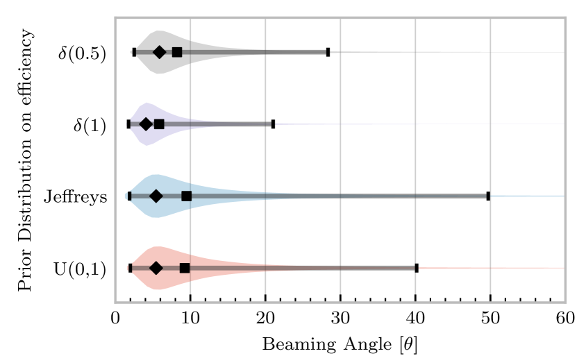
Figure 5: Beaming angle posteriors using different priors on SGRB efficiency $\epsilon$ in the 2015–2016 observing scenario.

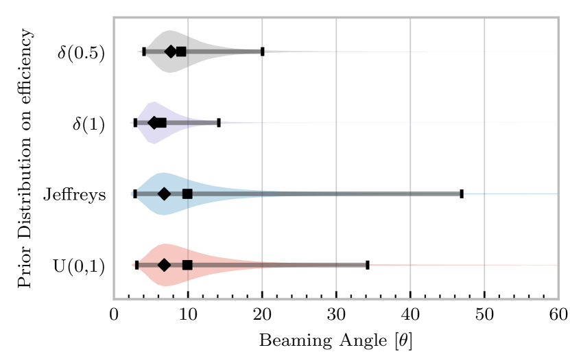
Figure 6: Beaming angle posteriors using different priors on SGRB efficiency $\epsilon$ in the 2016–2017 observing scenario.

Figures 5 and 6 show the beaming angle posteriors obtained for two of the detection scenarios. Since it is a common assumption in related literature, we also now include a prior on the SGRB efficiency which dictates that all NS–NS produce a SGRB, $p(\epsilon|I)=\delta(\epsilon=1)$, as well as our previous strong $\delta$-function prior. For the 2016-2017 scenario where inferences are somewhat weak (i.e., broad posteriors) due to the sparsity of GW detections, the uncertainties are large enough that the results from each prior are broadly consistent. In the 2024+ scenario, where the posterior is more peaked, it is clear that the strong $\delta$-function priors lead to inconsistent inferences on the SGRB beaming angle. The much weaker uniform and $\beta$ distributions, by contrast, are again largely consistent with each other yielding more conservative and robust results, as well as being a more representative expression of our state of knowledge. The inferences drawn from each scenario and each prior are summarised in terms of the maximum a posteriori measurement and the 95% credible interval around the maximum in table 5.

Scenario	Prior	Lower	MAP	Median	Upper
		[∘]	[∘]	[∘]	[∘]
2015–2016	U(0,1)	2.00	5.43	9.24	40.17
	Jeffreys	1.90	5.43	9.50	49.71
	$\delta(1)$	1.76	4.07	5.83	21.04
	$\delta(0.5)$	2.51	5.88	8.22	28.35
2016–2017	U(0,1)	3.09	6.78	9.91	34.23
	Jeffreys	2.85	6.78	9.91	46.93
	$\delta(1)$	2.88	5.43	6.40	14.15
	$\delta(0.5)$	4.06	7.69	9.07	20.05
2018–2019	U(0,1)	6.64	12.66	16.36	46.96
	Jeffreys	6.31	11.76	15.88	57.48
	$\delta(1)$	6.36	9.95	10.97	18.35
	$\delta(0.5)$	8.98	14.02	15.55	26.15
2020+	U(0,1)	8.20	12.66	16.04	44.73
	Jeffreys	7.82	12.21	15.35	56.99
	$\delta(1)$	8.10	10.85	11.12	14.95
	$\delta(0.5)$	11.47	14.92	15.75	21.17
2024+	U(0,1)	9.05	13.12	16.07	45.10
	Jeffreys	8.58	12.21	15.28	56.30
	$\delta(1)$	9.09	11.31	11.30	14.02
	$\delta(0.5)$	12.82	15.83	16.00	19.82

Table 5: Summary of the beaming angle inferences for each prior in each of the observing scenarios detailed in table 1. The lower and upper values correspond to the lower and upper bounds of the 95% Bayesian credible interval for each scenario.

5 Beaming Angle Constraints With No GW Detections

While GW170817 provided a situation where GW signals from a NS–NS coalescence event were observed, our proposed approach is also valid in the regime where no GW signals from NS–NS coalescence have been observed, as was true during the first observing run of the advanced LIGO detectors when upper limits on binary merger rates were used to place lower limits on the beaming angle Abbott et al. (2016a).

In this scenario, our procedure is identical to before: construct the posterior probability density function on the NS–NS coalescence rate, transform to the joint posterior on the beaming angle and SGRB efficiency, $\epsilon$, and marginalise over the nuisance parameter $\epsilon$ to yield the posterior on the beaming angle. Now, however, rather than quoting the maximum a posteriori estimate, together with some credible interval, we simply integrate the beaming angle posterior from $\theta=0$ until we reach that value which contains some desired confidence. Thus, we obtain an upper limit on the beaming angle, analogous to the rate upper limits set by past LIGO observations Abadie et al. (2012b).

Figure 5 shows the four posteriors on the beaming angle, corresponding to the four priors on the SGRB efficiency, $\epsilon$, using the observing 2015–2016 observing scenario from table 1, which corresponds closely to the conditions of the first science run of the advanced generation of ground based GW detectors. We define the upper limit on the beaming angle as the upper limit of the 95% credible interval where the credible interval is defined as the narrowest interval $(\theta^{\mathrm{ll}},\theta^{\mathrm{ul}})$ which satisfies the expression

$$0.95=\int_{\theta_{\mathrm{ll}}}^{\theta^{\mathrm{ul}}}p(\theta|D,I)~{}{\mathrm{d}}\theta,$$ (15)

with $p(\theta|D,I)$ the posterior over which the interval is computed.

Similarly we define the lower limit as the lower limit (2.5 percentile) of the same credible interval. In this non-detection scenario, we choose to compute upper limit on the 95% credible interval on the beaming angle.

We see that here, where the rate posterior is rather uninformative, the results are dominated by the uncertainty in $\epsilon$: there are substantive differences in the beaming angle upper limits yielded by the uniform ($U(0,1)$) and $\beta$-distribution priors, while the $\delta$-function priors yield dramatically different upper limits. Indeed, the most stringent (and mutually incompatible) upper limits are obtained using the strong $\delta$-function priors. In fact, these beaming angle upper limits are also incompatible with the values of $3^{\circ}\mbox{-}8^{\circ}$ that have been inferred from observations of jet breaks in SGRB afterglows Fong et al. (2014); Panaitescu (2006); Nicuesa Guelbenzu et al. (2012). Recall, however, from the discussion in section 2 that we interpret the beaming angle inference from our rate measurements as the upper bound on the mean of a population of beaming angles. It would, therefore, seem premature to conclude that there is tension in these results; instead, we can only state that either the population of SGRBs have a distribution of beaming angles with some finite width or that the fraction of NS–NS mergers which yield a SGRB is smaller than 0.5.

It is also interesting to compare these upper limits on the beaming angle with those in Chen & Holz (2013), where the upper limit on the rate itself is used as a constraint (rather than transforming the posterior). This has the important implication that the constraint thus obtained is the smallest angle consistent with the rate:

$$1-\cos\theta\geq\frac{{{\mathcal{R}}_{\mathrm{grb}}}}{\epsilon{{\mathcal{R}}}^{\mathrm{ul}}},$$ (16)

where ${{\mathcal{R}}}^{\mathrm{ul}}$ is the upper limit on the NS–NS rate. The same idea is used in Clark et al. (2015) to estimate beaming constraints in the advanced detector era. Thus, when comparing the constraints in e.g., Chen & Holz (2013) and the upper limits obtained from the transformed posterior (i.e., equation 10 and figure 7), one should remember that they are quite different quantities. There are two other noteworthy differences between Chen & Holz (2013) and this work: (i) the rate upper limit is computed based on the sensitivity of the initial LIGO-Virgo network (see e.g., Brady & Fairhurst (2008)), which gives ${{\mathcal{R}}}=4.5\times 10^{-4}$ Mpc^-3yr^-1 (as compared with ${{\mathcal{R}}}=1.3\times 10^{-4}$ Mpc^-3yr^-1 from the analysis in Abadie et al. (2012b)); and (ii) it is implicitly assumed that all NS–NS mergers yield an SGRB. That is, there is no factor or $\epsilon$ to account for the unknown fraction of mergers which successfully launch an SGRB jet. With these differences noted, the lower bound on the beaming angle is found to be $\theta\geq 0.8^{\circ}$, as compared with the lower limit of the 95% credible interval $\theta^{\mathrm{ll}}=1.76^{\circ}$ when assuming $\epsilon=1$, and the 2015-2016 observing scenario.

6 Beaming Angle Constraints in Future Scenarios

With the advent of gravitational wave astronomy, and with the expectation of the detection of NS–NS gravitational wave signals during the lifetime of the advanced detectors it will become possible to place further constraints on the 95% credible interval of the SGRB beaming angle, as both the searched 4-volume of space increases, and the observed rate of gravitational wave NS–NS events is established.

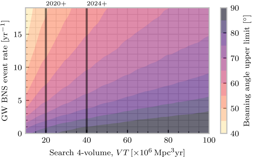
Figure 7: The upper-bound of the 95% credible interval on the beaming angle as a function of the rate of observed gravitational wave NS–NS events and the observed search 4-volume, taking a Jeffreys prior on the efficiency of GRB production from NS–NS events. The search volumes corresponding to observing scenarios are marked as vertical lines on the plot, with each line assuming that observations are carried out over the period of one year, achieving the search volume outlined in table 1.

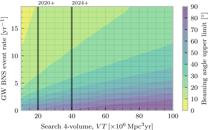
Figure 8: The upper-bound of the 95% credible interval on the beaming angle as a function of the rate of observed gravitational wave NS–NS events and the observed search 4-volume, assuming that all NS–NS events produce a GRB. The search volumes corresponding to observing scenarios are marked as vertical lines on the plot, with each line assuming that observations are carried out over the period of one year, achieving the search volume outlined in table 1.

In figure 7 we present the inferred upper-limit on the 95% credible interval for a range of search 4-volumes and gravitational wave event rates; overlayed on this plot are indications of the anticipated annual search volume for the advanced LIGO detectors in each of the observing scenarios detailed in table 1. These limits were determined by assuming a Jeffreys prior on the efficiency parameter of the model, and following the same procedure used to produce the posteriors in figures 5 and 6. In figure 8 we present a similar plot, showing the upper limits on the beaming angle under the stronger assumption that every NS–NS event also produces a GRB.

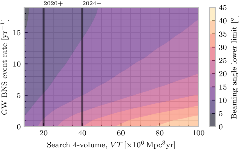
Figure 9: The lower-bound of the 95% credible limit on the beaming angle as a function of the observed number of events and the observed search 4-volume, taking a Jeffreys prior on the efficiency of GRB production from NS–NS events. The search volumes corresponding to observing scenarios are marked as vertical lines on the plot.

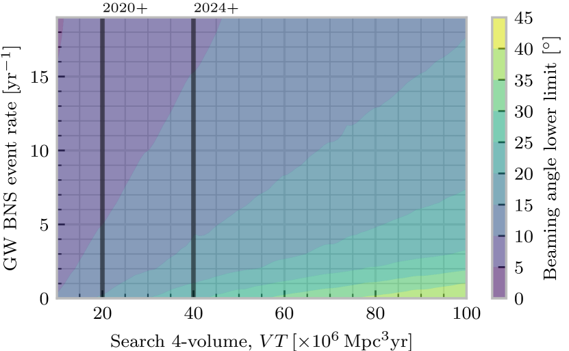
Figure 10: The lower-bound of the 95% credible limit on the beaming angle as a function of the observed number of events and the observed search 4-volume, assuming that every gravitational wave NS–NS event produces a GRB. The search volumes corresponding to observing scenarios are marked as vertical lines on the plot.

The lower limit (the 2.5% of the posterior) for the same range of scenarios is plotted in figure 9, with the same anticipated detector search volumes plotted, again assuming a Jeffreys prior on the efficiency, and in figure 10 we present those lower limits under the assumption that every NS–NS event produces a GRB.

7 Conclusion

We have presented a Bayesian analysis which demonstrates the ability of the current generation of advanced GW detectors to make observations that allow for the inference of SGRB jet beaming angles. In doing so we have made minimal assumptions about the processes which produce the jet, other than that NS–NS mergers are the progenitors and that, other than for rare nearby cases like GW170817, SGRBs are observed only by observers within the cone of the jet.

We demonstrate that with a year’s worth of gravitational wave observations by the 2-detector aLIGO network during its 2016-2017 observing run, and assuming a single NS–NS detection, that we can place a lower limit of $2.85^{\circ}$, and an upper limit of $46.93^{\circ}$ on the jet beaming angle, given an uninformative prior on the efficiency at which NS–NS events produce observable SGRBs. Assuming that all NS–NS produce an observable SGRBs we can narrow these limits to between $2.88^{\circ}$ and $14.15^{\circ}$.

When the advanced LIGO design sensitivity is acheived in 2020 the observation of 10 NS–NS events in gravitational waves is sufficient to place an upper limit of $56.99^{\circ}$ on the jet beaming angle, and can establishing the limit on the beaming angle to be between $7.82^{\circ}$ and $56.99^{\circ}$, assuming an uninformative prior on the SGRBs production efficiency. These limits narrow between $8.10^{\circ}$ and $14.95^{\circ}$ if perfect efficiency is assumed.

References

- Abadie et al. (2012a) Abadie, J., et al. 2012a, Astrophys. J., 755, 2
- Abadie et al. (2012b) —. 2012b, Phys. Rev., D85, 082002
- Abbott et al. (2008) Abbott, B., et al. 2008, Astrophys. J., 681, 1419
- Abbott et al. (2013) Abbott, B. P., et al. 2013, arXiv:1304.0670, [Living Rev. Rel.19,1(2016)]
- Abbott et al. (2016a) —. 2016a, Astrophys. J., 832, L21
- Abbott et al. (2016b) —. 2016b, Phys. Rev. Lett., 116, 061102
- Abbott et al. (2016c) —. 2016c, Phys. Rev. Lett., 116, 241103
- Abbott et al. (2017a) —. 2017a, Phys. Rev. Lett., 119, 161101
- Abbott et al. (2017b) —. 2017b, Astrophys. J., 848, L13
- Abbott et al. (2017) Abbott, B. P., Abbott, R., Abbott, T. D., et al. 2017, Astrophysical Journal Letters, 848, L12
- Abbott et al. (2017) Abbott, B. P., et al. 2017, Nature, arXiv:1710.05835
- Allen et al. (2012) Allen, B., Anderson, W. G., Brady, P. R., Brown, D. A., & Creighton, J. D. E. 2012, Phys. Rev. D, 85, 122006
- Blandford & Znajek (1977) Blandford, R. D., & Znajek, R. L. 1977, Mon. Not. Roy. Astron. Soc., 179, 433
- Blinnikov et al. (1984) Blinnikov, S. I., Novikov, I. D., Perevodchikova, T. V., & Polnarev, A. G. 1984, SvAL, 10, 177
- Brady & Fairhurst (2008) Brady, P. R., & Fairhurst, S. 2008, Classical and Quantum Gravity, 25, 105002
- Bromberg et al. (2013) Bromberg, O., Nakar, E., Piran, T., & Sari, R. 2013, Astrophys. J., 764, 179
- Chen & Holz (2013) Chen, H.-Y., & Holz, D. E. 2013, Phys. Rev. Lett., 111, 181101
- Clark et al. (2015) Clark, J., Evans, H., Fairhurst, S., et al. 2015, Astrophys. J., 809, 53
- Dal Canton et al. (2014) Dal Canton, T., et al. 2014, Phys. Rev., D90, 082004
- Dietz (2011) Dietz, A. 2011, Astron. Astrophys., 529, A97
- Eichler et al. (1989) Eichler, D., Livio, M., Piran, T., & Schramm, D. N. 1989, Nature, 340, 126
- Fong et al. (2014) Fong, W., Berger, E., Metzger, B. D., et al. 2014, Astrophys. J., 780, 118
- Fong et al. (2017) Fong, W., et al. 2017, Astrophys. J., 848, L23
- Fong et al. (2015) Fong, W.-f., Berger, E., Margutti, R., & Zauderer, B. A. 2015, Astrophys. J., 815, 102
- Galama et al. (1998) Galama, T. J., et al. 1998, Nature, 395, 670
- Giacomazzo et al. (2013) Giacomazzo, B., Perna, R., Rezzolla, L., Troja, E., & Lazzati, D. 2013, Astrophys. J., 762, L18
- Goldstein et al. (2017) Goldstein, A., et al. 2017, Astrophys. J., 848, L14
- Gottlieb et al. (2017) Gottlieb, O., Nakar, E., Piran, T., & Hotokezaka, K. 2017, arXiv:1710.05896
- Gregory (2010) Gregory, P. 2010, Bayesian Logical Data Analysis for the Physical Sciences
- Haggard et al. (2017) Haggard, D., Nynka, M., Ruan, J. J., et al. 2017, Astrophys. J., 848, L25
- Hunter (2007) Hunter, J. D. 2007, Computing In Science & Engineering, 9, 90
- Kasliwal et al. (2017) Kasliwal, M. M., et al. 2017, Science, arXiv:1710.05436
- Kouveliotou et al. (1993) Kouveliotou, C., Meegan, C. A., Fishman, G. J., et al. 1993, Astrophys. J., 413, L101
- Lee & Ramirez-Ruiz (2007) Lee, W. H., & Ramirez-Ruiz, E. 2007, New J. Phys., 9, 17
- LIGO Scientific Collaboration & Virgo Collaboration (2010) LIGO Scientific Collaboration, & Virgo Collaboration. 2010, Classical and Quantum Gravity, 27, 173001. http://stacks.iop.org/0264-9381/27/i=17/a=173001
- MacFadyen & Woosley (1999) MacFadyen, A., & Woosley, S. E. 1999, Astrophys. J., 524, 262
- Nakar (2007) Nakar, E. 2007, Phys. Rept., 442, 166
- Narayan et al. (1992) Narayan, R., Paczynski, B., & Piran, T. 1992, Astrophys. J., 395, L83
- Nicuesa Guelbenzu et al. (2012) Nicuesa Guelbenzu, A., Klose, S., Krühler, T., et al. 2012, Astronomy and Astrophysics, 538, L7
- Nissanke et al. (2010) Nissanke, S., Holz, D. E., Hughes, S. A., Dalal, N., & Sievers, J. L. 2010, Astrophys. J., 725, 496
- Nitz et al. (2017) Nitz, A., Harry, I., Brown, D., et al. 2017, ligo-cbc/pycbc: O2 Production Release 17, , , doi:10.5281/zenodo.844934. https://doi.org/10.5281/zenodo.844934
- Paczyński (1991) Paczyński, B. 1991, Acta Astron., 41, 257
- Panaitescu (2006) Panaitescu, A. 2006, Monthly Notices of the Royal Astronomical Society, 367, L42
- Pannarale & Ohme (2014) Pannarale, F., & Ohme, F. 2014, Astrophys. J., 791, L7
- Rosswog & Ramirez-Ruiz (2002) Rosswog, S., & Ramirez-Ruiz, E. 2002, Mon. Not. Roy. Astron. Soc., 336, L7
- Salvatier et al. (2016a) Salvatier, J., Wiecki, T. V., & Fonnesbeck, C. 2016a, PeerJ Computer Science, 2, e55
- Salvatier et al. (2016b) —. 2016b, PeerJ Computer Science, 2, e55. http://dblp.uni-trier.de/db/journals/peerj-cs/peerj-cs2.html#SalvatierWF16
- Savchenko et al. (2017) Savchenko, V., et al. 2017, Astrophys. J., 848, L15
- Schutz (1986) Schutz, B. F. 1986, Nature, 323, 310
- Usman et al. (2016) Usman, S. A., et al. 2016, Class. Quant. Grav., 33, 215004
- van der Walt et al. (2011) van der Walt, S., Colbert, S. C., & Varoquaux, G. 2011, Computing in Science & Engineering, 13, 22. http://aip.scitation.org/doi/abs/10.1109/MCSE.2011.37
- Woosley & Bloom (2006) Woosley, S. E., & Bloom, J. S. 2006, Ann. Rev. Astron. Astrophys., 44, 507
- Zhang et al. (2009) Zhang, B., et al. 2009, Astrophys. J., 703, 1696