Comparison of different concurrences characterizing photon-pairs generated in the biexciton cascade in quantum dots coupled to microcavities

Abstract

We compare three different notions of concurrence to measure the polarization entanglement of two-photon states generated by the biexciton cascade in a quantum dot embedded in a microcavity. The focus of the paper lies on the often-discussed situation of a dot with finite biexciton binding energy in a cavity tuned to the two-photon resonance. Apart from the time-dependent concurrence, which can be assigned to the two-photon density matrix at any point in time, we study single- and double-time integrated concurrences commonly used in the literature that are based on different quantum state reconstruction schemes. In terms of the photons detected in coincidence measurements, we argue that the single-time integrated concurrence can be thought of as the concurrence of photons simultaneously emitted from the cavity without resolving the common emission time, while the more widely studied double-time integrated concurrence refers to photons that are neither filtered with respect to the emission time of the first photon nor with respect to the delay time between the two emitted photons. Analytic and numerical calculations reveal that the single-time integrated concurrence indeed agrees well with the typical value of the time-dependent concurrence at long times, even when the interaction between the quantum dot and longitudinal acoustic phonons is accounted for. Thus, the more easily measurable single-time integrated concurrence gives access to the physical information represented by the time-dependent concurrence. However, the double-time integrated concurrence shows a different behavior with respect to changes in the exciton fine structure splitting and even displays a completely different trend when the ratio between the cavity loss rate and the fine structure splitting is varied while keeping their product constant. This implies the non-equivalence of the physical information contained in the time-dependent and single-time integrated concurrence on the one hand and the double-time integrated concurrence on the other hand.

I Introduction

Many applications in quantum communication require the generation of entangled photon pairs Gisin et al. (2002); O’Brian et al. (2009); Orieux et al. (2017); Zeilinger (2017); Versteegh et al. (2014); Müller et al. (2014). One particularly promising way of producing such pairs consists of using the biexciton cascade in quantum dots Akopian et al. (2006); Stevenson et al. (2006); Hudson et al. (2007); Hafenbrak et al. (2007); Stevenson et al. (2008); Bounouar et al. (2018); Pfanner et al. (2008); Sánchez Muñoz et al. (2015); Orieux et al. (2017), which can be sketched roughly as follows: An initially prepared biexciton state of a quantum dot decays to one of two possible single exciton states while emitting a photon. A second photon can be emitted while the quantum dot relaxes to its ground state. Because of the optical selection rules, the two different paths lead to an emission of either two horizontally or two vertically polarized photons. As the biexciton decay is a quantum mechanical process the system will, in general, be in a superposition of states from both paths. If both paths are completely symmetric, one expects that there is a high probability to find the system in the fully entangled state $|\psi^{+}\rangle=\frac{1}{\sqrt{2}}\big{(}|HH\rangle+|VV\rangle\big{)}$, where $|HH\rangle$ ($|VV\rangle$) denotes the state where the quantum dot is in its ground state and two horizontally (vertically) polarized photons have been emitted.

However, the situation in real quantum dots often deviates from the ideal picture described above. First of all, the exchange interaction typically introduces an energetic splitting between the two excitonic states on the order of several tens to hundreds of µeV Akopian et al. (2006); Mar et al. (2016); Bennett et al. (2010). Thus, the two paths become asymmetric, leading to a deviation from the usually desired state $|\psi^{+}\rangle$. Besides effects related to the fine structure splitting another source for deviations from the ideal situation are environment couplings, in particular to phonons. These couplings lead to decoherence and relaxation and are the reason why the system has to be represented by a mixed rather than a pure state. These detrimental effects can be suppressed by engineering the quantum dot devices accordingly. For example, the fine structure splitting between the excitonic states can be reduced by applying electrical Mar et al. (2016); Bennett et al. (2010) or strain fields Seidl et al. (2006) or by growing quantum dots within highly symmetric structures such as nanowires Huber et al. (2014). Here, we consider another approach to obtain more symmetric paths, which is achieved by embedding the quantum dot in a microcavity. Then, the coupling between the electronic states in the dot and the cavity modes leads to an overall faster dynamics, which reduces the time available for dephasing processes. Furthermore, tuning the cavity modes to the two-photon resonance between the ground and the biexciton state of the dot enhances two-photon processes that are much less affected by the splitting of the excitonic states than successive single-photon processes del Valle et al. (2011); Schumacher et al. (2012).

The wide interest in entanglement is twofold: on the one hand the occurrence of entanglement is one of the key differences between classical and quantum physics and on the other hand it has practical implications as it provides new ways of control as needed, e.g., for establishing secure quantum communication protocols Liao et al. (2018). The essence of the control aspect is that by performing a measurement on one part of the system one determines the outcome of measurements on another part of the system which otherwise would have been undetermined. If, e.g., the system is in the maximally entangled (non-factorizable) state $|\psi^{+}\rangle$ and one detects the polarization of one of the photons to be $H$, the state collapses into the factorized state $|HH\rangle$ and a polarization measurement on the second photon will necessarily yield $H$.

In order to compare two arbitrary states with respect to the amount of control obtainable by performing measurements as described above, one needs a measure of entanglement. For a pure state $|\Psi\rangle$ in a bipartite system with density matrix $\rho$ and parts $A$ and $B$ with reduced density matrices $\rho_{A}=\mathrm{Tr}_{B}\rho$ and $\rho_{B}=\mathrm{Tr}_{A}\rho$, respectively, it is common to define the entanglement $E(|\Psi\rangle)$ using the von-Neumann entropies of the subsystems Bennett et al. (1996):

$$E(|\Psi\rangle)=-\mathrm{Tr}_{A}\Big{(}\rho_{A}\log_{2}\rho_{A}\Big{)}=-\mathrm{Tr}_{B}\Big{(}\rho_{B}\log_{2}\rho_{B}\Big{)},$$ (1)

where the second equality in Eq. (1) follows from the Schmidt decomposition Nielsen and Chuang (2000). This entropy represents the missing information about a subsystem because of its entanglement with the other. Performing a measurement on one of the subsystems that collapses the system state into a factorizable state causes the subsystem entropy to drop to zero such that the previously missing information $E(|\Psi\rangle)$ is recovered. Therefore, $E(|\Psi\rangle)$ can also be considered to be a measure of the possible amount of control over subsystem $A$ by performing measurements on $B$.

For a mixed state missing information on a subsystem can arise due to its entanglement with the remaining part of the system as well as because of the ensemble averaging. There are a number of proposals to identify the corresponding contribution resulting from entanglement Bennett et al. (1996); Wootters (2001). Probably the most common proposal is the entanglement of formation. For a decomposition

$$\rho=\sum_{j}p_{j}\,|\Psi_{j}\rangle\langle\Psi_{j}|$$ (2)

of a density matrix $\rho$ with probabilities $p_{j}$ and not necessarily orthogonal states $|\Psi_{j}\rangle$ one assigns the entanglement:

$$E(\rho,\{p_{j},|\Psi_{j}\rangle\})=\sum_{j}p_{j}\,E(|\Psi_{j}\rangle).$$ (3)

Then the entanglement of formation is defined as:

$$E_{f}(\rho)=\inf\,E(\rho,\{p_{j},|\Psi_{j}\rangle\}),$$ (4)

where the infimum is taken over all possible decompositions in the form of Eq. (2). Thus, $E_{f}(\rho)$ represents the amount of pure-state entanglement that is at least present in a mixed state described by a given density matrix $\rho$. The entanglement of formation is particularly attractive because, unlike most other proposed measures of entanglement, it can be evaluated directly from the elements of the density matrix. To this end usually the concurrence $C$ is introduced which is related to the entanglement of formation by

$$E_{f}(\rho)=\mathcal{E}\big{(}C(\rho)\big{)},$$ (5)

where $\mathcal{E}$ is monotonically increasing for $0\leq C\leq 1$ (cf. Ref. Wootters, 2001 for an explicit expression for $\mathcal{E}$). Due to the monotonicity of $\mathcal{E}$ the concurrence is a measure of the entanglement of formation in its own right. Although the concurrence is less intuitive than the entanglement of formation and its physical interpretation derives only from its relation to $E_{f}(\rho)$, it is particularly attractive for practical applications because, as shown by Wootters Wootters (1998), it can be easily calculated from the elements of $\rho$ without having to perform a search for the infimum over all possible decompositions of $\rho$.

In the case of the biexciton cascade where no direct transitions between the two exciton states occur, the (unnormalized) density matrix in the two-photon subspace

$$\rho_{ij,kl}(t)=\langle a^{\dagger}_{i}(t)a^{\dagger}_{j}(t)a_{k}(t)a_{l}(t)\rangle,$$ (6)

with $a^{\dagger}_{i}(t)$ and $a_{l}(t)$ being the cavity photon creation and annihilation operators with polarization directions $i,j,k,l\in\{H,V\}$ in the Heisenberg picture, has only four non-vanishing elements, namely $\rho_{HH,HH},\rho_{VV,VV},\rho_{HH,VV}$, and $\rho_{VV,HH}$. Since we are dealing with a system where the photon number is not conserved, $\rho_{ij,kl}(t)$ has not unit trace for all times. The non-vanishing elements of the normalized density matrix can be represented accordingly by:

$$\rho^{N}_{j,l}(t)=\frac{\rho_{jj,ll}(t)}{\rho_{HH,HH}(t)+\rho_{VV,VV}(t)}.$$ (7)

The general expression for the concurrenceWootters (1998) then reduces to the normalized coherences between the states $|HH\rangle$ and $|VV\rangle$, which correspond to horizontal $H$ or vertical $V$ polarization of the emitted photons, i.e.:

$$C(t)=2|\rho^{N}_{H,V}(t)|.$$ (8)

Thereby, the concurrence relates two conceptually distinct properties of quantum systems: entanglement, which specifies how much the measurement of one qubit influences the measurement outcome of the second qubit, and coherence, which determines, e.g., the visibility of interference effects. A theoretical study where the time-dependent concurrence, which is assigned to the density matrix in the two-photon subspace at a given time, has been used as a figure of merit for entanglement has been performed, e.g., in Ref. Hein et al., 2014. However, in contrast to the investigation here, in Ref. Hein et al., 2014 the coupling of the dot to a continuum of half-space photon modes has been considered.

Although the elements of the density matrix are in principle all observable, it is often difficult to resolve their full time dependence experimentally and thereby determine the time-dependent concurrence given by Eq. (8). To reconstruct the two-photon density matrix from experimental data, one usually uses quantum state tomography, a technique based on polarization-dependent photon coincidence measurements James et al. (2001); Troiani et al. (2006). Because these coincidence measurements typically give only information about the polarization degree of freedom and the time delay $\tau$ between the two measured photons, but do not resolve the time $t$ of the first photon count with respect to the preparation of the biexciton state ($t=0$), in such experiments one only has access to quantities integrated over the time $t$. Therefore, studies of the photon pairs generated via the biexciton cascade often define figures of merit, which are then also called concurrence, but replace the density matrix in Eq. (8) by the respective expressions obtained from the quantum state reconstruction. The latter involve in general averages over $t$ and $\tau$. Most often discussed is the limiting case of long averaging intervals for both times Schumacher et al. (2012); Heinze et al. (2017); Pfanner et al. (2008). However, also the case where the averaging window for $t$ is infinite, while for $\tau$ the limit of a vanishing averaging interval is approached, is experimentally accessible Stevenson et al. (2008); Bounouar et al. (2018) and has been studied theoretically Carmele and Knorr (2011); del Valle (2013).

That these figures of merit may indeed differ substantially because of the differences in time averaging can be readily seen from the following argument due to Stevenson et al. Stevenson et al. (2008). Consider a biexciton cascade where an initially prepared biexciton decays to an exciton while emitting a single photon. A second photon is emitted after a delay time $\tau$, during which the different exciton states aquire a phase difference $\phi=\tau\delta/\hbar$ due to the fine structure splitting $\delta$. Disregarding environment influences which lead to a mixed photon state and concentrating only on the free time evolution the resulting two-photon state is $|\Psi\rangle=\frac{1}{\sqrt{2}}\big{(}|HH\rangle+e^{i\tau\delta/\hbar}|VV\rangle\big{)}$. Obviously, $|\Psi\rangle$ is a maximally entangled state at each point in time for any given delay. If, however, measurements are performed that do not discriminate between different delay times $\tau$ of the emission, the effective time-integration leads to significant cancellations of the phases $e^{i\tau\delta/\hbar}$. Stevenson et al.Stevenson et al. (2008) have performed experiments where the probability for finding the maximally entangled state $|\Psi\rangle=\frac{1}{\sqrt{2}}(|HH\rangle+|VV\rangle)$ in the two-photon state generated via the biexciton cascade has been determined as a function of the integration window for the delay time $\tau$. Indeed, it was found that this probability significantly drops the longer the $\tau$ sampling interval is taken. Thus, filtering photon pairs with nearly equal emission times reveals a high degree of entanglement while measurements involving long $\tau$ sampling times indicate a much lower entanglement. A similar experimental analysis has been recently performed by Bounouar et al.Bounouar et al. (2018) where it was concluded that the main limit of entanglement fidelity is the time resolution in the experiment.

The goal of this article is to compare the definitions of concurrences commonly used in the literature involving either single- or double-time averages with the time-dependent concurrence given by Eq. (8). To be specific, we study the case of the biexciton cascade in a quantum dot inside a microcavity. Concentrating at first on a model without phonons, we derive analytic expressions for the different concurrences for a quantum dot with finite biexciton binding energy in a cavity tuned to the two-photon resonance, a configuration which was already found to be favorable for a high degree of polarization entanglementSchumacher et al. (2012). The analytic results are valid also beyond the weak-coupling limit and agree qualitatively with numerical calculations. We find that the concurrence based on a single-time integrated two-photon density matrix yields very similar results as the time-dependent concurrence in Eq. (8). It is therefore possible to access the information represented by the time-dependent concurrence, i.e., the entanglement of formation contained in the so prepared state of the cavity photons, by recording the more easily measurable single-time integrated concurrence. This remains true even when the interaction between the quantum dot states and longitudinal acoustic phonons is taken into account in numerical calculations. However, this information cannot be accessed by measuring two-time integrated correlation functions since it turns out that the latter exhibit quantitatively and qualitatively different dependencies on parameters like the fine structure splitting. It is most striking that when comparing single- and double-time integrated concurrences even trends reverse, such as the dependence on the cavity loss rate in the presence of phonons. Furthermore, already without phonons, these two quantities show a completely reversed trend when the ratio between the cavity loss rate and the fine structure splitting is varied while their product is kept constant. This leads to the conclusion that the single-time integrated and the double-time integrated concurrence are measures for different types of entanglement.

II System

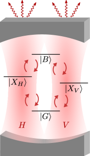
Figure 1: Sketch of the quantum dot states involved in the biexciton cascade inside a microcavity. The quantum dot is coupled to a microcavity with two orthogonally polarized cavity modes ($H$: horizontal, $V$: vertical). Due to optical selection rules, the biexciton state ($|B\rangle$) can be deexcited to one of two exciton states ($|X_{H}\rangle$ and $|X_{V}\rangle$) under the emission of a $H$ or $V$ polarized cavity photon. The exciton states can be further deexcited to the ground state ($|G\rangle$) of the dot by emitting a second photon. The reverse processes are also possible. The red circular arrows indicate the dot-cavity coupling compatible with the optical selection rules. Wavy arrows symbolize the photon losses due to the imperfect cavity.

II.1 Hamiltonian

We consider a quantum dot in a microcavity as depicted in Fig. 1. We assume that the quantum dot is initialized at time $t=0$ in the biexciton state with an empty cavity, e.g., by incoherent excitation from the wetting layer or direct laser excitation. The biexciton is coupled to two quantum states with an exciton in the quantum dot and a photon in the cavity. The two excitons are labeled by $X_{H}$ and $X_{V}$ corresponding to the polarization of the cavity mode, horizontal ($H$) or vertical ($V$), to which the respective transition is coupled. The excitonic states are also coupled to the ground state of the dot with one more photon in the cavity. At the same time, the cavity is subject to losses and the excitons in the dot interact with longitudinal acoustic (LA) phonons. Radiative decay is assumed to be negligible compared with cavity losses, which is a typical case Reithmaier et al. (2004).

The dot-cavity Hamiltonian is given by Heinze et al. (2017)

$$H_{dc}= \;\big{(}\hbar\bar{\omega}_{X}+\frac{\delta}{2}\big{)}|X_{H}\rangle\langle X_{H}|+\big{(}\hbar\bar{\omega}_{X}-\frac{\delta}{2}\big{)}|X_{V}\rangle\langle X_{V}|$$

$$+\big{(}2\hbar\bar{\omega}_{X}-E_{B}\big{)}|B\rangle\langle B|+\hbar\omega_{H}a^{\dagger}_{H}a_{H}+\hbar\omega_{V}a^{\dagger}_{V}a_{V}$$

$$+\hbar g\Big{[}\big{(}|G\rangle\langle X_{H}|+|X_{H}\rangle\langle B|\big{)}a^{\dagger}_{H}$$

$$+\big{(}|G\rangle\langle X_{V}|-|X_{V}\rangle\langle B|\big{)}a^{\dagger}_{V}$$

$$+\big{(}|X_{H}\rangle\langle G|+|B\rangle\langle X_{H}|\big{)}a_{H}$$

$$+\big{(}|X_{V}\rangle\langle G|-|B\rangle\langle X_{V}|\big{)}a_{V}\Big{]},$$ (9)

where $\hbar\bar{\omega}_{X}$ is the average exciton energy, $\delta$ is the fine structure splitting and $E_{B}$ is the biexciton binding energy. The energies of the cavity modes are $\hbar\omega_{H}$ and $\hbar\omega_{V}$, respectively, and $g$ is the dot-cavity coupling constant. Here, we assume that the cavity modes are in resonance with the two-photon transition between the ground and the biexciton state $\hbar\omega_{H}=\hbar\omega_{V}=\frac{2\hbar\bar{\omega}_{X}-E_{B}}{2}$. $|G\rangle$ denotes the ground state of the dot, $|X_{H}\rangle$ and $|X_{V}\rangle$ are the exciton states, and $|B\rangle$ is the biexciton state. Finally, $a^{\dagger}_{i}$ ($a_{i}$) is the creation (annihilation) operator for a photon in the cavity mode $i=\{H,V\}$.

Cavity losses are taken into account via the Lindblad term

$$\mathcal{L}_{\textrm{cavity}}[\rho]=\frac{\kappa}{2}\sum_{i=H,V}\big{(}2a_{i}\rho a^{\dagger}_{i}-a^{\dagger}_{i}a_{i}\rho-\rho a^{\dagger}_{i}a_{i}\big{)},$$ (10)

where $\kappa$ is the cavity loss rate. The interaction between the dot and the LA phonons is described by the Hamiltonian

$$\hat{H}_{ph}=\hbar\!\sum_{\mathbf{q}}\omega_{\mathbf{q}}{b}^{\dagger}_{\mathbf{q}}{b}_{\mathbf{q}}+\hbar\!\sum_{\mathbf{q}}\sum_{\nu}n^{X}_{\nu}\big{(}\gamma_{\mathbf{q}}^{X}{b}^{\dagger}_{\mathbf{q}}+\gamma_{\mathbf{q}}^{X*}{b}_{\mathbf{q}}\big{)}|\nu\rangle\langle\nu|,$$ (11)

where $b^{\dagger}_{\mathbf{q}}$ and $b_{\mathbf{q}}$ are the creation and annihilation operators for phonons with wave vectors $\mathbf{q}$ and energies $\hbar\omega_{\mathbf{q}}$. $n^{X}_{\nu}=\{0,1,1,2\}$ is the number of excitons in the dot state $\nu=\{G,X_{H},X_{V},B\}$ and $\gamma_{\mathbf{q}}^{X}$ is the exciton-phonon coupling constant.

II.2 Concurrences

The time-dependent concurrence which has been shown by Wootters Wootters (1998) to be a measure for the entanglement of formation is, for the two-photon state created in the biexciton cascade, given by Eq. (8). Since the density matrix in this equation is evaluated with cavity operators [cf. Eq. (6)], it immediately follows that $C(t)$ contains information about the entanglement of formation of the two-photon state inside the cavity at any given time $t$. Experimentally, the reduced two-photon density matrix is typically reconstructed via quantum state tomography, where polarization-resolved two-photon coincidence rates are measured which are proportional to the two-time correlation functions

$$G^{(2)}_{ij,kl}(t,\tau)=\langle a_{i}^{\dagger}(t)a_{j}^{\dagger}(t+\tau)a_{k}(t+\tau)a_{l}(t)\rangle.$$ (12)

Here, $t$ is the time of the first click at a detector, $\tau$ is the delay time until the second photon is detected and $i,j,k,l\in\{H,V\}$. Since in experiments one measures photons that have left the cavity, the cavity operators in Eq. (12) should in fact be replaced by operators for the field modes outside the cavity. However, considering the outcoupling of light out of the cavity to be a Markovian process, the quantities measured outside the cavity are proportional to the ones insideKuhn et al. (2016). Therefore, a measurement of $G^{(2)}_{ij,kl}(t,\tau)$ outside the cavity can indeed be described by Eq. (12). Finally, we note that in the present analysis we have assumed the radiative decay to be negligible compared with the cavity losses and, consequently, we only consider the case that photons are emitted via the cavity. For a direct emission of photons into modes outside the cavity by radiative decay, two-time correlation functions involving polarization operators instead of photon operators would have to be considered Troiani et al. (2006).

Typically, corresponding experiments record data points over extended time intervals $t_{0}\leq t\leq t_{0}+\Delta t$ and $\tau_{0}\leq\tau\leq\tau_{0}+\Delta\tau$. For the reconstruction of the unnormalized density matrix defined in Eq. (6) the delay line between the two detectors measuring the coincidence is adjusted such that the two intervals where the detectors are sensitive start simultaneously, i.e. $\tau_{0}=0$. Setting $t_{0}=0$ the measured signals are then proportional to

$$\overline{\overline{G}}^{(2)}_{ij,kl}(\Delta t,\Delta\tau)=$$

$$\frac{1}{\Delta t\,\Delta\tau}\int_{0}^{\Delta t}dt\int_{0}^{\Delta\tau}d\tau\;\langle a_{i}^{\dagger}(t)a_{j}^{\dagger}(t+\tau)a_{k}(t+\tau)a_{l}(t)\rangle.$$ (13)

Thus, the result of an experimental reconstruction of the normalized two-photon density matrix is Troiani et al. (2006)

$$\rho^{R}_{j,l}(\Delta t,\Delta\tau)=\frac{\overline{\overline{G}}^{(2)}_{jj,ll}(\Delta t,\Delta\tau)}{\overline{\overline{G}}^{(2)}_{HH,HH}(\Delta t,\Delta\tau)+\overline{\overline{G}}^{(2)}_{VV,VV}(\Delta t,\Delta\tau)}.$$ (14)

Associated with the reconstructed density matrix is the concurrence

$$C^{R}(\Delta t,\Delta\tau)=2|\rho^{R}_{H,V}(\Delta t,\Delta\tau)|.$$ (15)

As low counting rates limit the experimental accuracy, common measurements are performed using rather long intervals for the data collection. These experiments often approach the limiting case $\Delta t\to\infty$ and $\Delta\tau\to\infty$ such that in theory the corresponding concurrence becomesSchumacher et al. (2012); Heinze et al. (2017)

$$\overline{\overline{C}}=\lim_{\begin{subarray}{c}\Delta t\to\infty\\ \Delta\tau\to\infty\end{subarray}}C^{R}(\Delta t,\Delta\tau).$$ (16)

Due to the double-time averaging, the information about the time evolution of the system is completely lost such that, in contrast to the time dependent concurrence $C(t)$, the double-time integrated concurrence $\overline{\overline{C}}$ does not reflect properties of the cavity photons at any given time but rather describes the properties of the reconstructed density matrix in experiments.

While the case of extended measuring intervals for both $t$ and $\tau$ is probably the most often discussed situation, in the literature also another limiting case has been considered Carmele and Knorr (2011); del Valle (2013), where the concurrence is defined as

$$\overline{C} =\lim_{\begin{subarray}{c}\Delta t\to\infty\\ \Delta\tau\to 0\end{subarray}}C^{R}(\Delta t,\Delta\tau).$$ (17)

Experimentally, the limit $\Delta\tau\to 0$ can be performed using time-windowing techniques Stevenson et al. (2008) which record signals over different delay-time windows $\Delta\tau$ and extrapolate to $\Delta\tau=0$. More recently it has been shown experimentally that using time bins with a width of $4\,$ps is sufficient to resolve the full $\tau$ dependence of the signal if the exciton fine-structure splitting is on a scale of a few tens of µeVBounouar et al. (2018). Henceforth, we refer to the concurrence $\overline{C}$ defined in Eq. (17) as the single-time integrated concurrence. If the photon pairs are emitted from a dot-cavity system in the steady state, $\overline{C}$ is equivalent to $C(t)$ since the two-photon density matrix no longer depends on time in such a case. However, when considering dynamical systems that are, e. g., driven by laser pulses, this equivalence in general no longer holds.

It should be noted that, as for the time-dependent concurrence $C(t)$, also for the single-time integrated concurrence $\overline{C}$ it is not necessary to evaluate the two-time correlation function defined in Eq. (12) since in the limit $\Delta\tau\to 0$ only the unnormalized density matrix given by Eq. (6) enters the expression in Eq. (17). However, one should be aware that $\overline{C}$ is not the time average of the time-dependent concurrence $C(t)$. Instead, the time average of the concurrence is given by

$$\langle C\rangle_{T} :=\frac{1}{T}\int_{0}^{T}dt\,C(t)$$

$$=\frac{1}{T}\int_{0}^{T}dt\,\frac{2|\rho_{HH,VV}(t)|}{\rho_{HH,HH}(t)+\rho_{VV,VV}(t)},$$ (18)

where $T$ corresponds to the averaging time.

In the following we shall compare the time-dependent concurrence $C(t)$, which measures the entanglement of formation of the two-photon system inside the cavity at a given point in time, with the double- and single-time integrated concurrences $\overline{\overline{C}}$ and $\overline{C}$, respectively, obtained as a result of different quantum state reconstruction strategies that involve data collection over extended time intervals. Due to the one-to-one correspondence between two-time correlation functions of photon operators inside and outside the cavity shown in Ref. Kuhn et al., 2016, the comparison between $C(t)$, $\overline{C}$, and $\overline{\overline{C}}$ can also be interpreted in terms of the photons recorded in the two detectors used in coincidence measurement. Since the photons outside the cavity propagate with the speed of light they can be recorded at a given time in one of the detectors only when they have been emitted from the cavity at a retarded time that matches the flight time between cavity and detector. Thus, recording the correlation function $G^{(2)}_{ij,kl}(t,\tau)$ for given values of $t$ and $\tau$ selects photons according to their emission time from the cavity. Note that for the photons inside the cavity there is no obvious relation between their emission times from the dot since standing wave modes localized in the cavity are excited and thus these excitations contribute to the two-time correlation functions as long as the photons stay in the cavity.

The above analysis suggests that a density matrix constructed from the two-time correlation function for given values of $t$ and $\tau$, i.e. $\rho_{j,l}(t,\tau)=\frac{G^{(2)}_{jj,ll}(t,\tau)}{G^{(2)}_{HH,HH}(t,\tau)+G^{(2)}_{VV,VV}(t,\tau)}$, represents a measurement of photons in two detectors where the photons are selected according to their respective emission times from the cavity. Then, $C(t,\tau)=2|\rho_{H,V}(t,\tau)|$ can be interpreted as a measure for the entanglement of formation of the so selected photons. The question now arises how to interpret the quantity $C^{R}(\Delta t,\Delta\tau)$ defined in Eq. (15), which is obtained by first taking a coherent superposition of signal contributions associated with different emission times and then constructing the concurrence by taking twice the absolute value of the off-diagonal element of the normalized superposition. At this point it is helpful to discuss in more detail the emission process from the cavity. If we were dealing with an ensemble of randomly distributed emission events where each emission has a sharply defined emission time $t_{e}$ and where the uncertainty concerning the emission time is described by a classical probability distribution for $t_{e}$, then the concurrence of this ensemble would be obtained by first evaluating the concurrence separately for each ensemble member, which would be $C(t,\tau)=2|\rho_{H,V}(t,\tau)|$, and then averaging over the emission times, i.e., $t$ and $\tau$. The result would be an average concurrence similar to $\langle C\rangle_{T}$ except that here the average would be taken over $t$ and $\tau$. However, in a full quantum description, the uncertainty concerning the emission times is not represented by a classical ensemble of events with sharp emission times. Instead, states where a photon has been emitted are typically in a coherent superposition with states where no photon has been emitted. Thus, the emission is not point-like in time but is a process of finite duration, so that $\overline{\overline{G}}^{(2)}_{ij,kl}(\Delta t,\Delta\tau)$ can be thought of as filtering out the coherent superposition corresponding to those contributions where the emission times are restricted to $t$ and $\tau$ intervals of lengths $\Delta t$ and $\Delta\tau$, respectively. This means that $C^{R}(\Delta t,\Delta\tau)$ represents the concurrence associated with a reconstructed two-photon density matrix which is filtered with respect to emission times within finite intervals. From this point of view, $C(t)$ represents the concurrence of photons recorded in two detectors that are simultaneously (i.e. $\tau=\Delta\tau=0$) emitted from the cavity at a given time $t$, while $\overline{C}$ also describes the concurrence of simultaneously emitted photons but without resolving their common emission time. Finally, $\overline{\overline{C}}$ is the concurrence associated with a two-photon density matrix where one neither resolves the emission time of the first recorded photon nor the delay time $\tau$ between the photons.

III Time-dependent concurrence

In the following, we first present an approximate analytic expression for the time-dependent concurrence of the two-photon state generated by the biexciton cascade in a dot-cavity system in the absence of dot-phonon interaction. Subsequently, we compare the anayltic results with numerical calculations of the time-dependent concurrence as well as the single-time integrated concurrence with and without dot-phonon interaction.

III.1 Analytic results

In order to discuss how the time-dependent concurrence $C(t)$ depends on the parameters of the system, it is instructive to look for an approximate analytic solution of the dynamics in the absence dot-phonon interaction.

First, note that only few states contribute to the biexciton cascade: The general states of the system can be described by $|\nu,n_{H},n_{V}\rangle$, where $\nu\in\{G,X_{H},X_{V},B\}$ denotes the dot state and $n_{H}$ and $n_{V}$ are the numbers of horizontally and vertically polarized cavity photons, respectively. Without losses and under the assumption that the system is initially prepared in the biexciton state $|B,0,0\rangle$ and not driven externally, the number of total excitations (number of excitons plus number of photons) in the system is fixed to two for all times. When accounting for losses via the Lindblad operator defined in Eq. (10), also states with excitation numbers smaller than two become occupied. However, these states need not be considered for the subsequent dynamics since first, they do not contribute to the two-photon density matrix $\rho_{ij,kl}(t)$ defined in Eq. (6) and second, states with lower excitation numbers do not couple back to states with higher excitation numbers. Since there are no direct transitions between the different excitons $X_{H}$ and $X_{V}$ or between horizontally and vertically polarized photons, only five remaining states contribute, which we denote by

$$|G_{H}\rangle:=|G,2,0\rangle,$$ (19a)

$$|G_{V}\rangle:=|G,0,2\rangle,$$ (19b)

$$|X_{H}\rangle:=|X_{H},1,0\rangle,$$ (19c)

$$|X_{V}\rangle:=|X_{V},0,1\rangle,$$ (19d)

$$|B\rangle:=|B,0,0\rangle.$$ (19e)

In this basis, the Hamiltonian in Eq. (9) takes the form

$$H=\left(\begin{array}[]{ccccc}0&0&\sqrt{2}\hbar g&0&0\\ 0&0&0&\sqrt{2}\hbar g&0\\ \sqrt{2}\hbar g&0&\frac{1}{2}(E_{B}+\delta)&0&\hbar g\\ 0&\sqrt{2}\hbar g&0&\frac{1}{2}(E_{B}-\delta)&-\hbar g\\ 0&0&\hbar g&-\hbar g&0\end{array}\right),$$ (25)

where the origin of the energy scale is shifted to the biexciton.

An analytic solution of the full five-level system is complicated and has so far only been presented in the weak coupling limit Carmele and Knorr (2011) ($g\ll\kappa$), where only one-way transitions along the paths $|B\rangle\to|X_{H}\rangle\to|G_{H}\rangle$ and $|B\rangle\to|X_{V}\rangle\to|G_{V}\rangle$ can occur because the photon losses are much faster than the time needed for the reexcitation of higher-energetic dot states. However, to fully benefit from the microcavity one is often interested in strongly coupled dot-cavity systemsSchneider et al. (2016); Reithmaier (2008); Kasprzak et al. (2013) where the condition $g\ll\kappa$ is not met and other approaches are required.

Here, we make use of the fact that in typical quantum dots the biexciton binding energy $E_{B}\sim 1-6$ meV defines the largest energy scale. Strongly coupled dot-cavity systems typically have couplings on the order of $\hbar g\sim 0.1$ meV while typical values for the fine structure splitting are in the range of $\delta\sim 0.01-0.1$ meV, so that a perturbative treatment in terms of the small parameters $\lambda:=\hbar g/(\frac{1}{2}E_{B})$ and $\delta/E_{B}$ is appropriate. For later reference we also define $\lambda_{H/V}:=\hbar g/[\frac{1}{2}(E_{B}\pm\delta)]$.

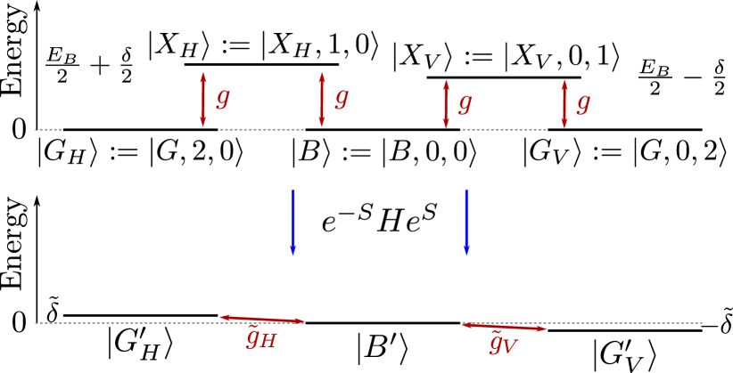
Figure 2: Sketch of the block diagonalization reducing the dynamics in the five-level system described in Eqs. (19) to a three-level system with states defined in Eqs. (30).

In the case considered here, where the cavity modes are in resonance with the two-photon transition to the biexciton state, the comparatively large binding energy suppresses the occupation of the exciton states. Thus, one can perform a perturbative block-diagonalization Winkler (2003); Bravyi et al. (2011) (Schrieffer-Wolff transformation) and thereby remove the high-energy states with one exciton and one photon from the dynamics, as sketched in Fig. 2. To this end a unitary transform $e^{-S}He^{S}$ is applied to the Hamiltonian $H$, where $S=S^{(1)}+S^{(2)}+\dots$ is expanded in orders of the perturbing Hamiltonian $H^{(1)}$ consisting of the off-diagonal elements of $H$ in Eq. (25). The matrices $S^{(i)}$ are then obtained by the condition that the matrix elements between high- and low-energy states in $e^{-S}He^{S}$ vanish up to order $\mathcal{O}\big{(}(H^{(1)})^{i+1}\big{)}$ (cf. Refs. Winkler, 2003 or Bravyi et al., 2011 for explicit expressions for $S^{(i)}$). This transformation therefore perturbatively eliminates the couplings between the low-energy ground- and biexciton-like states and the high-energy exciton-like states. After decoupling the low-energy and high-energy states, the latter are disregarded as they are irrelevant for the dynamics.

Up to second order in $\lambda$, the block-diagonalization yields the effective Hamiltonian

$$H^{\prime}=\left(\begin{array}[]{ccc}\tilde{\delta}&0&\hbar\tilde{g}_{H}\\ 0&-\tilde{\delta}&\hbar\tilde{g}_{V}\\ \hbar\tilde{g}_{H}&\hbar\tilde{g}_{V}&0\end{array}\right),$$ (29)

with $\tilde{\delta}=\hbar g(\lambda_{V}-\lambda_{H})\approx\lambda^{2}\delta$ and $\tilde{g}_{H/V}=\mp\sqrt{2}\lambda_{H/V}g$ in the basis

$$|G^{\prime}_{H}\rangle:= \big{(}1-\lambda_{H}^{2}\big{)}|G_{H}\rangle-\sqrt{2}\lambda_{H}|X_{H}\rangle-\frac{1}{\sqrt{2}}\lambda_{H}^{2}|B\rangle,$$ (30a)

$$|G^{\prime}_{V}\rangle:= \big{(}1-\lambda_{V}^{2}\big{)}|G_{V}\rangle-\sqrt{2}\lambda_{V}|X_{V}\rangle+\frac{1}{\sqrt{2}}\lambda_{V}^{2}|B\rangle,$$ (30b)

$$|B^{\prime}\rangle:= -\frac{\lambda_{H}^{2}}{\sqrt{2}}|G_{H}\rangle+\frac{\lambda_{V}^{2}}{\sqrt{2}}|G_{V}\rangle-\lambda_{H}|X_{H}\rangle+\lambda_{V}|X_{V}\rangle$$

$$+\big{(}1-\frac{1}{2}(\lambda_{H}^{2}+\lambda_{V}^{2})\big{)}|B\rangle.$$ (30c)

Thus, perturbation theory in $\lambda$ allows one to reduce the five-level system of the biexciton cascade to an effective three-level system, where the three levels have mostly the character of the ground state of the dot with two horizonally or vertically polarized photons and the biexciton state.

In the three-level basis, the effective coupling $\tilde{g}_{H/V}$ is reduced by a factor $\sim\lambda$ compared with the coupling $g$ in the five-level system. The effective splitting $2\tilde{\delta}$ between the states $|G^{\prime}_{H}\rangle$ and $|G^{\prime}_{V}\rangle$ is reduced even more compared with the fine structure splitting $\delta$ of the excitonic states in the original five-level system because it only appears in second order in $\lambda$. When also the Lindblad terms are written in the basis described in Eq. (30), the biexciton-like state $|B^{\prime}\rangle$ acquires the small loss rate $(\lambda_{H}^{2}+\lambda_{V}^{2})\kappa$ and the loss rates for the states $|G^{\prime}_{H}\rangle$ and $|G^{\prime}_{V}\rangle$ become $2(1-\lambda_{H/V}^{2})\kappa$, which are of the same order of magnitude as the rates $\kappa$ for the corresponding states $|G_{H}\rangle$ and $|G_{V}\rangle$ in the five-level system.

The central insight gained by this transformation is that, due to the renormalization of the coupling, the effective three-level system can be in the weak coupling limit $|\tilde{g}_{H/V}|\ll\kappa$ even when the orignal five-level system describing the biexciton cascade is not $(g\sim\kappa)$, as is the case for typical parameters for dot-cavity systems Schumacher et al. (2012). Due to the weak coupling, the dynamics in the effective three-level system is easily understood: The initial occupations of the biexciton state $|B^{\prime}\rangle$ are transferred to the ground states $|G^{\prime}_{H}\rangle$ and $|G^{\prime}_{V}\rangle$ and then decay due to the losses before they can reexcite the biexciton state, yielding an essentially incoherent dynamics. An explicit calculation of the dynamics in the weakly coupled effective three-level system is presented in appendix A. It is found that the occupation of the biexciton-like state $|B^{\prime}\rangle$ decays exponentially with an effective rate

$$\kappa_{B}=(\lambda_{H}^{2}+\lambda_{V}^{2})\left(\frac{4g^{2}}{\kappa}+\kappa\right),$$ (31)

where the term propotional to ${4g^{2}}/{\kappa}$ is due to the transitions to the states $|G^{\prime}_{H}\rangle$ and $|G^{\prime}_{V}\rangle$ and the term proportional to $\kappa$ originates from the losses due to the admixture of states with a nonvanishing number of photons to the state $|B^{\prime}\rangle$. The occupations and coherences $\rho_{G^{\prime}_{i}G^{\prime}_{j}}=\langle\big{(}|G^{\prime}_{i}\rangle\langle G^{\prime}_{j}|\big{)}\rangle$ between the states $|G^{\prime}_{H}\rangle$ and $|G^{\prime}_{V}\rangle$ are found to be

$$\rho_{G^{\prime}_{i}G^{\prime}_{j}}=\frac{\tilde{g}_{i}\tilde{g}_{j}}{\kappa^{2}}\left(e^{-\kappa_{B}t}-e^{[-(2-\lambda_{i}^{2}-\lambda_{j}^{2})\kappa+i(\tilde{\delta}_{i}-\tilde{\delta}_{j})/\hbar]t}\right),$$ (32)

with $\tilde{\delta}_{H/V}=\pm\tilde{\delta}$.

The long-time dynamics of $\rho_{G^{\prime}_{i}G^{\prime}_{j}}$ is determined by the same loss rate $\kappa_{B}$ as the biexciton-like state, whereas the initial increase from zero is governed by a term decaying with $\kappa\gg\kappa_{B}$. Because the renormalized splitting $\tilde{\delta}$ is very small compared with typical loss rates $\kappa$, possible oscillations of $\rho_{G^{\prime}_{H}G^{\prime}_{V}}$ are overdamped. Furthermore, the second term in Eq. (32) disappears already after a short time $\sim\kappa^{-1}$. Neglecting $\tilde{\delta}$ in the second exponent in Eq. (32) yields the following simple analytic expression for the concurrence

$$C_{\textrm{analytic}}=\frac{2|\rho_{G^{\prime}_{H}G^{\prime}_{V}}|}{\rho_{G^{\prime}_{H}G^{\prime}_{H}}+\rho_{G^{\prime}_{V}G^{\prime}_{V}}}\approx\frac{2|\tilde{g}_{H}\tilde{g}_{V}|}{\tilde{g}_{H}^{2}+\tilde{g}_{V}^{2}}=\frac{E_{B}^{2}-\delta^{2}}{E_{B}^{2}+\delta^{2}}.$$ (33)

First, we find that, although the density matrix elements change in time, the analytic expression predicts that the concurrence is constant in time. Furthermore, the concurrence depends only on the biexciton binding energy and the fine structure splitting and is indepedent of the dot-cavity coupling $g$ and the cavity loss rate $\kappa$.

Because all density matrix elements entering in the expression for the concurrence have virtually the same time dependence, integrating the density matrix elements over the time $t$ yields the same result also for the single-time integrated concurrence

$$\overline{C}_{\textrm{analytic}}=C_{\textrm{analytic}}\approx\frac{E_{B}^{2}-\delta^{2}}{E_{B}^{2}+\delta^{2}}.$$ (34)

Thus, our analysis reveals that the single-time integrated concurrence is the same as the concurrence at any point in time and is therefore a measure of the entanglement of formation for the two-photon state generated in the cavity by the biexciton cascade.

III.2 Numerical results

To check the validity of the analytic results for the concurrence, we now present numerical calculations of the biexciton cascade described by the dot-cavity Hamiltonian in Eq. (9) and the loss term in Eq. (10) in the five-level basis introduced in Eq. (19). Futhermore, we study the effects of phonons due to the dot-phonon Hamiltonian in Eq. (11), which have been neglected in the derivation of the analytic results, using a numerically exact real-time path-integral method Makri and Makarov (1995); Vagov et al. (2011); Barth et al. (2016); Cygorek et al. (2017) described in detail in the supplement of Ref. Cygorek et al., 2017.

If not stated otherwise, we use the following parameters: dot-cavity coupling constant $\hbar g=0.1$ meV, biexciton binding energy $E_{B}=1.5$ meV, cavity loss rate $\kappa=0.25$ ps^-1, and fine structure splitting $\delta=0.1$ meV. Note that for these parameters ($g/\kappa\approx 0.6$) the system is clearly not in the weak-coupling limit, so that conventional weak-coupling theories are not applicable. For calculations involving the dot-phonon interaction, we use parameters suitable for a 3 nm wide self-assembled InGaAs quantum dot embedded in a GaAs matrix (cf. Ref. Cygorek et al., 2017). Furthermore, the phonons are assumed to be initially in equilibrium at a temperature $T=10$ K.

Figure 3 depicts the time evolution of the time-dependent concurrence $C(t)$ and the single-time integrated concurrence $\overline{C}$ determined numerically as well as its analytic value according to Eq. (34). In the absence of dot-phonon interaction, the time-dependent concurrence indeed agrees well with the constant analytic result as well as the single-time integrated concurrence after an initial phase of $\sim 40$ ps duration, as expected from the analytic results. If phonons are taken into account, $C(t)$ and $\overline{C}$ still agree well after this initial phase, but the stationary value for long times is reduced.

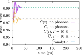
Figure 3: Time-dependent concurrence $C(t)$ and single-time integrated concurrence $\overline{C}$ calculated numerically without dot-phonon interaction and with phonons at a temperature $T=10$ K compared with the analytically obtained result $C_{\textrm{analytic}}$ for the phonon-free case.

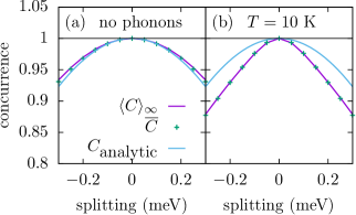
Figure 4: Dependence of the time-averaged concurrence $\langle C\rangle_{\infty}$, and the single-time integrated concurrence $\overline{C}$ on the fine structure splitting $\delta$, calculated (a) without dot-phonon interaction and (b) with phonons at a temperature $T=10$ K. For comparison the analytically obtained result $C_{\textrm{analytic}}$ for the phonon-free case is displayed in (a) and (b).

The dependence of the time-averaged concurrence $\langle C\rangle_{\infty}$ and the single-time integrated concurrence $\overline{C}$ on the fine structure splitting $\delta$ is shown in Fig. 4. Here, we consider $\langle C\rangle_{\infty}$ since it condenses the information contained in $C(t)$ into a single number that can be compared with $\overline{C}$. The averaging time $T=1000$ ps for $\langle C\rangle_{\infty}$ is chosen such that it is much larger compared with all other timescales in the system. For calculations not accounting for the dot-phonon interaction [Fig. 4(a)], the time-averaged concurrence and the single-time integrated concurrence are in good agreement with the analytic results for the whole range of fine structure splittings. When phonons are taken into account [Fig. 4(b)], both definitions of the concurrence still coincide but yield, in general, significantly lower values than the concurrence obtained by neglecting the dot-phonon interaction. However, at vanishing fine structure splitting $\delta=0$, the concurrence remains one even in the presence of phonons as predicted in previous studiesCarmele and Knorr (2011). This is due to the fact that both paths of the biexciton cascade are completely symmetric in this case. The resulting absence of which-way information makes it possible to get a completely entangled state for all times.

It is worth noting that the value of the concurrence remains close to one even for the relatively large fine structure splitting of $\delta=0.1$ meV. As will be discussed in Sec. IV, the dependence of the double-time integrated concurrence on $\delta$ turns out to be completely different. The near independence on $\delta$ of the single-time integrated concurrence is easily understood by the argument of Stevenson et al. Stevenson et al. (2008) discussed in the introduction according to which there is a high probability for finding the maximally entangled state $|\Psi\rangle=\frac{1}{\sqrt{2}}\big{(}|HH\rangle+e^{i\tau\delta/\hbar}|VV\rangle\big{)}$. Thus, the time-dependent as well as the single-time integrated concurrence have high values because even for finite $\delta$ the system is at any point in time close to a maximally entangled state. This high degree of entanglement can, however, not be uncovered when the system state is reconstructed by collecting data points over an extended $\tau$ interval, as is done in the double-time integrated concurrence, because of destructive interference. The remaining observed weak decrease of the single-time integrated concurrence with rising $\delta$ reflects the deviation of the actual system state from the idealized pure state $|\Psi\rangle$.

Finally, the dependence of $\langle C\rangle_{\infty}$ and the single-time integrated concurrence $\overline{C}$ on the cavity loss rate $\kappa$ is depicted in Fig. 5 for a fine structure splitting $\delta=0.1$ meV. Again, in absence of dot-phonon interaction, the time-averaged concurrence as well as the single-time integrated concurrence coincide with the analytic result, which is independent of $\kappa$. When the interaction between the quantum dot and the phonons is accounted for, it is found that the concurrence increases monotonically with increasing loss rate. At $\kappa=0$, the concurrence becomes zero (not shown) and for large loss rates, the concurrence approaches the same value as obtained when the dot-phonon interaction is disregarded. This can be explained by the fact that the dot-phonon interaction enables phonon-assisted processes. First of all, given enough time, phonon emission and absorption leads to a thermal occupation of energy eigenstates. Secondly, transitions involving the exciton states $|X_{H},1,0\rangle$ and $|X_{V},0,1\rangle$, which are otherwise off-resonant, are enabled by the absorption of phonons with energies close to $E_{B}/2$. For typical biexciton binding energies in the range of a few meV this energy is close to the maximum of typical phonon spectral density Glässl et al. (2013), so that the phonon-assisted transitions through excitonic states are particularly efficient. In any case, the coherences between the states $|G,2,0\rangle$ and $|G,0,2\rangle$ are strongly reduced by phonon effects, which in turn reduce the concurrence $C(t)$.

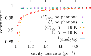
Figure 5: Dependence of the time-averaged concurrence $\langle C\rangle_{\infty}$ and the single-time integrated concurrence $\overline{C}$ with and without dot-phonon interaction on the cavity loss rate $\kappa$ using a fine structure splitting $\delta=0.1$ meV. Also shown is the analytically obtained result $C_{\textrm{analytic}}$.

However, the phonon-induced loss of coherence requires a finite amount of time and therefore competes with the cavity losses. Note that the latter leads to a uniform decrease of the coherences as well as the occupations of the two-photon state, which appear in the numerator and the denominator in the definition of the concurrence $C(t)$ in Eq. (8), respectively. Therefore, the cavity losses do not directly affect the concurrence $C(t)$, which is also the reason why the analytic expression $C_{\textrm{analytic}}$ in Eq. (33) does not depend on $\kappa$. In contrast, phonons only marginally affect the occupations but they can strongly reduce the coherences, which results in a reduced concurrence $C(t)$. Thus, if the cavity loss rate $\kappa$ is small, phonons can suppress the degree of entanglement measured by the concurrence $C(t)$. For large $\kappa$, the occupations can decay faster than the time needed for phonon-induced decoherence, so that for very large $\kappa$ the phonon-free situation is recovered.

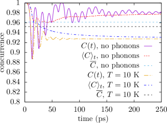
Figure 6: Time-dependent concurrence $C(t)$ and time-averaged concurrence $\langle C\rangle_{t}$ as a function of time plotted together with the value of the single-time integrated concurrence $\overline{C}$ for a quantum dot with a small biexciton binding energy $E_{B}=0.3$ meV with and without dot-phonon interaction.

To summarize, our numerical calculations of the concurrence in the biexciton cascade in the absence of dot-phonon interaction confirm the validity of the analytic expression for the concurrence in Eq. (33) for a large range of fine structure splittings and cavity loss rates. This supports the core idea of our analytic approach that the biexciton cascade can be discussed in terms of an effective three-level system that, when the biexciton binding energy is large enough, is in the weak-coupling limit ($\tilde{g}\ll\kappa$) even if the original system is not ($g\sim\kappa$). As a consequence of the weak coupling in the effective three-level system, the dynamics of the relevant two-photon density matrix elements is exponentially damped rather than oscillatory, so that an integration over time does not lead to a cancellation of coherences. For this reason, the single-time integrated concurrence $\overline{C}$ agrees very well with the typical value of the time-dependent concurrence $C(t)$ and its average value given by $\langle C\rangle_{\infty}$ and is therefore a measure for the entanglement of formation of the two-photon state. Numerically exact path integral calculations reveal that the relation $\overline{C}\approx\langle C\rangle_{\infty}$ still holds when the dot-phonon interaction is accounted for.

However, the quantitative agreement between $\overline{C}$ and the time-averaged concurrence $\langle C\rangle_{\infty}$ can also be brought to its limits: For systems with small or vanishing biexciton binding energy, $\lambda=\hbar g/(\frac{1}{2}E_{B})$ is no longer a small parameter, which has consequences for the time-dependent concurrence as can be seen in Fig. 6. For a small biexciton binding energy, the concurrence $C(t)$ shows pronounced oscillations that persist for more than $100$ ps if the influence of phonons is disregarded. When accounting for the dot-phonon interaction the oscillations are damped down much more quickly. These oscillations can be traced back to a coherent Rabi dynamics between the ground and the biexciton state which causes an oscillatory behavior for both the numerator and the denominator in the expression for $C(t)$ given by Eq. (8). If one compares in such a case the long-time limit of the time-averaged concurrence $\langle C\rangle_{\infty}$, which coincides reasonably well with $C(t)$ for long times, with the single-time integrated concurrence $\overline{C}$, where numerator and denominator are separately averaged over time, it is found that these quantities noticeably deviate.

IV Double-time integrated concurrence

Having discussed the time-dependent and single-time integrated concurrence, we now move on to the double-time integrated concurrence. To this end, we derive an analytic expression for the double-time integrated concurrence for the biexciton cascade in absence of dot-phonon interaction and subsequently compare it with numerical results.

IV.1 Analytic results

The calculation of the double-time integrated concurrence $\overline{\overline{C}}$ as defined in Eq. (16) requires the knowledge of the two-time correlation function $G^{(2)}_{ij,kl}(t,\tau)$, which can be obtained in the Heisenberg picture by

$$G^{(2)}_{ij,kl}(t,\tau)=\textrm{Tr}\big{[}a^{\dagger}_{i}(t)a^{\dagger}_{j}(t+\tau)a_{k}(t+\tau)a_{l}(t)\hat{\rho}(0)\big{]},$$ (35)

where $\hat{\rho}(0)$ is the initial density matrix. Introducing the time evolution operator $U(t)$ and rearranging terms yields

$$G^{(2)}_{ij,kl}(t,\tau)=\textrm{Tr}\big{[}a_{j}^{\dagger}a_{k}U(\tau)[a_{l}U(t)\hat{\rho}(0)U(-t)a_{i}^{\dagger}]U(-\tau)\big{]}.$$ (36)

To obtain the double-time integrated concurrence, we first integrate over the time $t$ and define

$$\overline{G}^{(2)}_{ij,kl}(\tau)=\int\limits_{0}^{\infty}dt\,G^{(2)}_{ij,kl}(t,\tau)=\textrm{Tr}\big{[}a_{j}^{\dagger}a_{k}U(\tau)\tilde{\rho}(0)U(-\tau)\big{]}$$

$$=\textrm{Tr}\big{[}a_{j}^{\dagger}(\tau)a_{k}(\tau)\tilde{\rho}(0)\big{]}=\langle a_{j}^{\dagger}a_{k}(\tau)\rangle_{\tilde{\rho}},$$ (37a)

with

$$\tilde{\rho}(0)=\int\limits_{0}^{\infty}dt\,a_{l}U(t)\hat{\rho}(0)U(-t)a_{i}^{\dagger}=a_{l}\bigg{[}\int\limits_{0}^{\infty}dt\,\hat{\rho}(t)\bigg{]}a_{i}^{\dagger}.$$ (37b)

Thus, $\overline{G}^{(2)}_{ij,kl}(\tau)$ can be calculated like the average of the operator $a_{j}^{\dagger}a_{k}$ at time $\tau$ evaluated with a generalized (possibly non-Hermitian) density matrix $\tilde{\rho}$. The initial value of $\tilde{\rho}$ can be obtained from the dynamics of the density matrix elements that have been calculated analytically in the last section. The matrix elements have to be integrated over the time $t$ and the photon operators $a_{l}$ and $a_{i}^{\dagger}$ have to be applied from the left and from the right, respectively. Note that to derive Eqs. (37) we have assumed a time evolution given by a unitary operator $U(t)$. In practice, we take into account a Lindblad term in the equations of motion for the description of cavity losses due to the coupling of the light modes within the cavity with a continuum of light modes outside the cavity. Such non-Hamitonian terms give rise to a dynamics that is, in general, not described by a unitary time evolution. However, when the light modes outside the cavity are included in the description, the time evolution of the total system can again be represented by a unitary time evolution operator $U(t)$. Calculating the trace in Eq. (37a) over the field modes outside of the cavity and applying the usual Markovian approximation for the derivation of the Lindblad equations it is straightforward to show that the abovementioned prescription for the calculation of $\overline{G}^{(2)}_{ij,kl}(\tau)$ identically transfers to systems with Lindblad terms such as cavity losses.

As before, it is easy to see that in order to calculate the concurrence, one only needs to account for matrix elements of $\hat{\rho}(t)$ involving the five states defined in Eqs. (19) with exactly two excitations. The application of the operators $a_{l}$ and $a_{i}^{\dagger}$ reduces the number of photons and thereby the number of excitations by one. Furthermore, the biexciton state without photons $|B,0,0\rangle$ is removed by the action of a photon destruction operator, leaving only the four relevant states

$$\tilde{G}_{H}= |G,1,0\rangle,$$ (38a)

$$\tilde{X}_{H}= |X_{H},0,0\rangle,$$ (38b)

$$\tilde{X}_{V}= |X_{V},0,0\rangle,$$ (38c)

$$\tilde{G}_{V}= |G,0,1\rangle$$ (38d)

that have to be accounted for in the calculation of $\tilde{\rho}(\tau)$. Restricted to this basis, the dot-cavity Hamiltonian reads

$$H=\left(\begin{array}[]{cccc}0&\hbar g&0&0\\ \hbar g&\frac{1}{2}(E_{B}+\delta)&0&0\\ 0&0&\frac{1}{2}(E_{B}-\delta)&\hbar g\\ 0&0&\hbar g&0\end{array}\right).$$ (43)

This Hamiltonian represents a system of two decoupled two-level systems, which is diagonalized by the eigenstates

$$\tilde{G}^{\prime}_{i}= \cos(\lambda_{i})|\tilde{G}_{i}\rangle-\sin(\lambda_{i})|\tilde{X}_{i}\rangle,$$ (44a)

$$\tilde{X}^{\prime}_{i}= \sin(\lambda_{i})|\tilde{G}_{i}\rangle+\cos(\lambda_{i})|\tilde{X}_{i}\rangle$$ (44b)

with $i\in\{H,V\}$. In order to get more transparent expressions, we again focus on terms up to second order in $\lambda$ and approximate $\cos(\lambda_{H/V})\approx 1-\frac{1}{2}\lambda_{H/V}^{2}$ as well as $\sin(\lambda_{H/V})\approx\lambda_{H/V}$. Then, the energy eigenvalues are

$$E_{\tilde{G}^{\prime}_{i}}= -\lambda_{i}^{2}\frac{1}{2}(E_{B}+\delta_{i}),$$ (45a)

$$E_{\tilde{X}^{\prime}_{i}}= (1+\lambda_{i}^{2})\frac{1}{2}(E_{B}+\delta_{i})$$ (45b)

with $\delta_{H/V}=\pm\delta$.

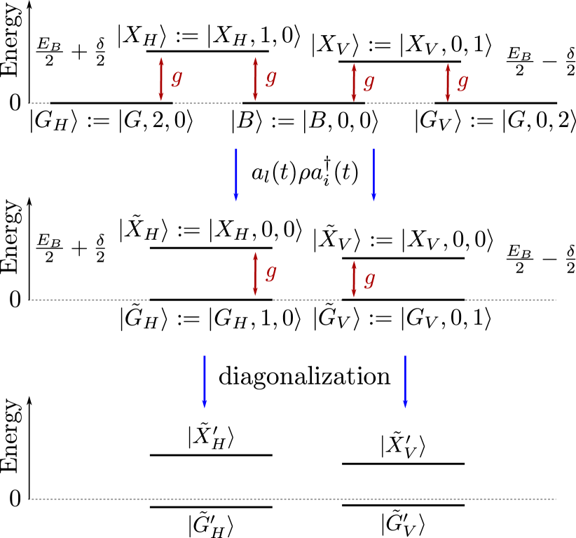
Figure 7: Sketch of the four-level system for the description of the $\tau$-dependence of the two-time correlation function $G^{(2)}_{ij,kl}(t,\tau)$. The application of $a_{l}$ from the left and $a_{i}^{\dagger}$ from the right on the density matrix $\rho$ with non-zero elements only for the five states depicted in the top panel results in a generalized density matrix with non-zero elements only for the four states in the middle panel. The resulting four-level system can be decomposed into two decoupled two-level systems and diagonalized analytically.

Transforming also the Lindblad term into the basis of the states in Eqs. (44), we obtain the equations of motion

$$\frac{\partial}{\partial\tau}\tilde{\rho}_{\tilde{G}^{\prime}_{i}\tilde{G}^{\prime}_{j}}= \big{[}\frac{i}{\hbar}(E_{\tilde{G}^{\prime}_{i}}-E_{\tilde{G}^{\prime}_{j}})-\kappa\big{(}1-\frac{1}{2}(\lambda_{i}^{2}+\lambda_{j}^{2})\big{)}\big{]}\tilde{\rho}_{\tilde{G}^{\prime}_{i}\tilde{G}^{\prime}_{j}}$$

$$-\frac{1}{2}\kappa\big{(}\lambda_{i}\tilde{\rho}_{\tilde{X}^{\prime}_{i}\tilde{G}^{\prime}_{j}}+\lambda_{j}\tilde{\rho}_{\tilde{G}^{\prime}_{i}\tilde{X}^{\prime}_{j}}\big{)},$$ (46a)

$$\frac{\partial}{\partial\tau}\tilde{\rho}_{\tilde{G}^{\prime}_{i}\tilde{X}^{\prime}_{j}}= \big{[}\frac{i}{\hbar}(E_{\tilde{G}^{\prime}_{i}}-E_{\tilde{X}^{\prime}_{j}})-\frac{1}{2}\kappa\big{(}1-\lambda_{i}^{2}+\lambda_{j}^{2})\big{)}\big{]}\tilde{\rho}_{\tilde{G}^{\prime}_{i}\tilde{X}^{\prime}_{j}}$$

$$-\frac{1}{2}\kappa\big{(}\lambda_{i}\tilde{\rho}_{\tilde{X}^{\prime}_{i}\tilde{X}^{\prime}_{j}}+\lambda_{j}\tilde{\rho}_{\tilde{G}^{\prime}_{i}\tilde{G}^{\prime}_{j}}\big{)},$$ (46b)

$$\frac{\partial}{\partial\tau}\tilde{\rho}_{\tilde{X}^{\prime}_{i}\tilde{X}^{\prime}_{j}}= \big{[}\frac{i}{\hbar}(E_{\tilde{X}^{\prime}_{i}}-E_{\tilde{X}^{\prime}_{j}})-\frac{1}{2}\kappa\big{(}\lambda_{i}^{2}+\lambda_{j}^{2})\big{)}\big{]}\tilde{\rho}_{\tilde{X}^{\prime}_{i}\tilde{X}^{\prime}_{j}}$$

$$-\frac{1}{2}\kappa\big{(}\lambda_{i}\tilde{\rho}_{\tilde{G}^{\prime}_{i}\tilde{X}^{\prime}_{j}}+\lambda_{j}\tilde{\rho}_{\tilde{X}^{\prime}_{i}\tilde{G}^{\prime}_{j}}\big{)}.$$ (46c)

Note that the cross terms introduced by the losses are of minor importance since the slowly changing occupations $\tilde{\rho}_{\tilde{G}^{\prime}_{i}\tilde{G}^{\prime}_{j}}$ and $\tilde{\rho}_{\tilde{X}^{\prime}_{i}\tilde{X}^{\prime}_{j}}$ are off-resonantly driven by the fast oscillating (with frequency $\sim\frac{1}{2}{E_{B}}/\hbar$) coherences $\tilde{\rho}_{\tilde{G}^{\prime}_{i}\tilde{X}^{\prime}_{j}}$ and vice versa. This allows us to neglect these cross terms in the following. Then, the solutions of Eqs. (46) are damped oscillations.

Here, we are interested in the delay-time-integrated matrices

$$\overline{\overline{\rho}}_{ij}=\int\limits_{0}^{\infty}d\tau\,\tilde{\rho}_{ij}(\tau),$$ (47)

which can be expressed by

$$\overline{\overline{\rho}}_{\tilde{G}^{\prime}_{i}\tilde{G}^{\prime}_{j}}= \frac{1}{\kappa\big{(}1-\frac{1}{2}(\lambda_{i}^{2}+\lambda_{j}^{2})\big{)}-\frac{i}{\hbar}\big{(}E_{\tilde{G}^{\prime}_{i}}-E_{\tilde{G}^{\prime}_{j}}\big{)}}\tilde{\rho}_{\tilde{G}^{\prime}_{i}\tilde{G}^{\prime}_{j}}(0),$$ (48a)

$$\overline{\overline{\rho}}_{\tilde{G}^{\prime}_{i}\tilde{X}^{\prime}_{j}}= \frac{1}{\frac{1}{2}\kappa\big{(}1-\lambda_{i}^{2}+\lambda_{j}^{2}\big{)}-\frac{i}{\hbar}\big{(}E_{\tilde{G}^{\prime}_{i}}-E_{\tilde{X}^{\prime}_{j}}\big{)}}\tilde{\rho}_{\tilde{G}^{\prime}_{i}\tilde{X}^{\prime}_{j}}(0),$$ (48b)

$$\overline{\overline{\rho}}_{\tilde{X}^{\prime}_{i}\tilde{X}^{\prime}_{j}}= \frac{1}{\frac{1}{2}\kappa\big{(}\lambda_{i}^{2}+\lambda_{j}^{2}\big{)}-\frac{i}{\hbar}\big{(}E_{\tilde{X}^{\prime}_{i}}-E_{\tilde{X}^{\prime}_{j}}\big{)}}\tilde{\rho}_{\tilde{X}^{\prime}_{i}\tilde{X}^{\prime}_{j}}(0).$$ (48c)

The final steps to obtain the double-time integrated concurrence are a number of basis transformations of the initial values: First, we have to transform the analytic result for the single-time averaged density matrix in the effective three-level system [basis: $G^{\prime}_{i},B^{\prime}$ in Eqs. (30)] back into the original five-level system [basis: $G_{i},X_{i},B$ in Eqs. (19)], then we have to apply the photon annihilation operators [new basis: $\tilde{G}_{i},\tilde{X}_{i}$ in Eqs. (38)] and transform the result to the diagonal basis spanned by the states $\tilde{G}^{\prime}_{i}$ and $\tilde{X}^{\prime}_{i}$ defined in Eqs. (44) to obtain the initial values for the effective density matrix $\tilde{\rho}_{ij}(0)$. With these initial values, Eqs. (48) are evaluated and the result is transformed back to the basis spanned by $\tilde{G}_{i}$ and $\tilde{X}_{i}$.

Keeping only second-order terms, we find the initial values:

$$\tilde{\rho}_{\tilde{G}^{\prime}_{i}\tilde{G}^{\prime}_{j}}(0)\approx \tilde{\rho}_{\tilde{G}_{i}\tilde{G}_{j}}(0)=4(2\delta_{ij}-1)\frac{g^{2}}{\kappa^{2}}\frac{\lambda_{i}\lambda_{j}}{\kappa_{B}},$$ (49a)

$$\tilde{\rho}_{\tilde{G}^{\prime}_{i}\tilde{X}^{\prime}_{j}}(0)\approx \tilde{\rho}_{\tilde{G}_{i}\tilde{X}_{j}}(0)=2i(2\delta_{ij}-1)\frac{g}{\kappa}\frac{\lambda_{i}\lambda_{j}}{\kappa_{B}},$$ (49b)

$$\tilde{\rho}_{\tilde{X}^{\prime}_{i}\tilde{X}^{\prime}_{j}}(0)\approx \tilde{\rho}_{\tilde{X}_{i}\tilde{X}_{j}}(0)=(2\delta_{ij}-1)\frac{\lambda_{i}\lambda_{j}}{\kappa_{B}}.$$ (49c)

The double-time integrated density matrix elements entering the concurrence are

$$\overline{\overline{\rho}}_{\tilde{G}_{i}\tilde{G}_{j}}\approx \frac{1-\frac{1}{2}(\lambda_{i}^{2}+\lambda_{j}^{2})}{\kappa\big{(}1-\frac{1}{2}(\lambda_{i}^{2}+\lambda_{j}^{2})\big{)}}\tilde{\rho}_{\tilde{G}_{i}\tilde{G}_{j}}(0)$$

$$+\frac{\lambda_{i}\lambda_{j}}{\frac{1}{2}\kappa(\lambda_{i}^{2}+\lambda_{j}^{2})-\frac{i}{\hbar}(E_{\tilde{X}^{\prime}_{i}}-E_{\tilde{X}^{\prime}_{j}})}\tilde{\rho}_{\tilde{X}_{i}\tilde{X}_{j}}(0)$$ (50)

because the coherences $\tilde{\rho}_{\tilde{G}^{\prime}_{i}\tilde{X}^{\prime}_{j}}$ lead to contributions of the order of $\mathcal{O}(\lambda^{3})$. Thus, the double-time integrated density matrix has two contributions, one from direct transitions through the low-energy eigenstates $\tilde{G}^{\prime}_{i}$ and one from transitions through the high-energy exciton-like eigenstates $\tilde{X}^{\prime}_{i}$. On the one hand, the contributions from the occupations $\tilde{\rho}_{\tilde{X}^{\prime}_{i}\tilde{X}^{\prime}_{j}}$ are suppressed by a factor $\sim\lambda^{2}$ because the projection of $\tilde{X}^{\prime}_{i}$ on $\tilde{G}_{i}$ is $\sim\lambda$. On the other hand, the losses for the exciton-like states $\tilde{X}^{\prime}_{i}$ are smaller by a factor $\sim\lambda^{2}$, so that the time integral yields a larger contribution. All in all, the relative strength of the contributions from transitions through $\tilde{G}^{\prime}_{i}$ and $\tilde{X}^{\prime}_{i}$ are determined by the factor $4g^{2}/\kappa^{2}$.

It is also interesting that the occupations of the exciton-like states $\tilde{X}^{\prime}_{i}$ stem from the projection of the occupations of biexciton-like eigenstate $B^{\prime}$ onto $|X_{H},1,0\rangle$ and $|X_{V},0,1\rangle$ at the time of the loss of the first photon, i.e., when the first photon annihilation operator is applied. In contrast, the contributions through $\tilde{G}^{\prime}_{i}$ have their origin in the occupations of the ground-states $|G,2,0\rangle$ and $|G,0,2\rangle$. This suggests that the latter can be interpreted as a two-photon process in the sense that two excitations are transferred from the quantum dot to the cavity before the first photon is emitted from the cavity, while the former corresponds to a one-photon process. This interpretation is corroborated by the fact that the factor $4g^{2}/\kappa^{2}$ is identical to the ratio $\kappa_{2P}/\kappa_{1P}$ between cavity-assisted two- and one-photon emission processes discussed in Ref. del Valle et al., 2011 in the context of the generation of highly polarized (nonentangled) photon pairs.

Using the analytic expressions for the double-time integrated density matrix $\overline{\overline{\rho}}$, the double-time integrated concurrence is found to be

$$\overline{\overline{C}}= \frac{2|\overline{\overline{\rho}}_{G_{H}G_{V}}|}{\overline{\overline{\rho}}_{G_{H}G_{H}}+\overline{\overline{\rho}}_{G_{V}G_{V}}}$$

$$= C_{\textrm{analytic}}\frac{\Big{|}4\frac{g^{2}}{\kappa^{2}}+C_{\textrm{analytic}}\frac{1}{1-ip}\Big{|}}{4\frac{g^{2}}{\kappa^{2}}+1}$$ (51)

with

$$p:=\frac{E_{\tilde{X}^{\prime}_{H}}-E_{\tilde{X}^{\prime}_{V}}}{\hbar\kappa\frac{1}{2}(\lambda_{H}^{2}+\lambda_{V}^{2})}.$$ (52)

Keeping only the lowest-order terms in $\lambda$ and $\frac{\delta}{E_{B}}$ in the numerator and in the denominator, we can further simplify this result to

$$p\approx\frac{\delta}{\hbar\kappa\lambda^{2}}=\frac{\delta E_{B}^{2}}{4\hbar^{3}\kappa g^{2}}.$$ (53)

Note that the contribution of $\frac{1}{1-ip}$ to the concurrence becomes insignificant for $\delta\gg\hbar\kappa\lambda^{2}$. Therefore, this term only contributes for small splittings $\delta$, for which the value of the concurrence $C_{\textrm{analytic}}$ is nearly one and the double-time integrated concurrence is well described by

$$\overline{\overline{C}}_{\textrm{analytic}}= C_{\textrm{analytic}}\frac{\sqrt{\Big{(}4\frac{g^{2}}{\kappa^{2}}+\frac{1}{1+p^{2}}\Big{)}^{2}+\Big{(}\frac{p}{1+p^{2}}\Big{)}^{2}}}{4\frac{g^{2}}{\kappa^{2}}+1}$$ (54)

with $p$ from Eq. (53).

IV.2 Numerical results

In Fig. 8, the numerically calculated double-time integrated concurrence $\overline{\overline{C}}$ for the phonon-free case is depicted as a function of the fine structure splitting $\delta$ for $\hbar g=0.1$ meV, $\kappa=0.25$ ps^-1, and $E_{B}=1.5$ meV and compared with the analytic expressions for the time-dependent and double-time integrated concurrence. The analytic expression for the double-time integrated concurrence reproduces the main features of the numerical results quite well. For further comparison we also show in Fig. 8 results for $\overline{\overline{C}}$ accounting for phonons at a temperature $T=10$ K. The necessary evaluation of two-time correlation functions in the presence of phonons has been carried out by a numerically exact path integral approach, the details of which will be discussed elsewhere.

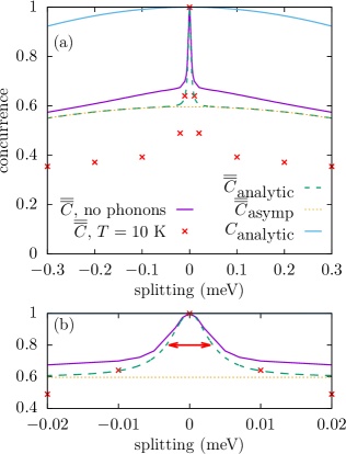
Figure 8: (a) Double-time integrated concurrence $\overline{\overline{C}}$ as a function of the fine structure splitting $\delta$ for the phonon-free case and with phonons for a temperature $T=10$ K compared with its analytic approximation $\overline{\overline{C}}_{\textrm{analytic}}$ in the phonon-free case and the corresponding asymptotic behavior $\overline{\overline{C}}_{\textrm{asymp}}$. Also shown is the analytic result $C_{\textrm{analytic}}$ for the single-time integrated concurrence without phonons. (b) shows a zoom of the central peak where the red double arrow indicates a FWHM of $2\hbar\kappa\lambda^{2}={8\hbar^{3}\kappa g^{2}}/{E_{B}^{2}}$.

Let us first concentrate on the results for the phonon-free case. In contrast to our analytic expression $C_{\text{analytic}}$, which approximates well the time-dependent concurrence $C(t)$ as seen before and which remains close to one even for large fine structure splittings, the double-time integrated concurrence $\overline{\overline{C}}$ typically has a narrow Lorentzian-like peak at splittings close to zero with a width $\sim 10$ µeV and, for larger splittings, reaches a plateau. This qualitative behavior of the double-time integrated concurrence has been reported before in numerical studies Schumacher et al. (2012); Heinze et al. (2017) and is also in agreement with experimental results Stevenson et al. (2006); Hudson et al. (2007); Hafenbrak et al. (2007). However, to the best of our knowledge, key quantities, such as the width of the central peak and the height of the plateau, have not yet been explained in terms of the microscopic parameters of the system. Here, the derivation of the analytic expression for the double-time integrated concurrence allows us to identify these key quantities. In particular, recall that the numerator in the analytic expression for the double-time integrated concurrence in Eq. (54) has two contributions: the terms containing the parameter $p$ originating from transitions through exciton-like energy eigenstates $\tilde{X}^{\prime}_{i}$ of the four-level system in Eqs. (38), and another term from the transitions through the lowest energy eigenstates $\tilde{G}^{\prime}_{i}$. Because $p$ is proportional to the fine structure splitting $\delta$ and the contribution through the exciton-like eigenstates $\tilde{X}^{\prime}_{i}$ decays for large values of $p$ as $\frac{1}{p}$, the double-time integrated concurrence for large $\delta$ is determined by the contribution through the eigenstates $\tilde{G}^{\prime}_{i}$. For $p\to\infty$, one obtains from the analytic expression in Eq. (54)

$$\overline{\overline{C}}_{\textrm{asymp}}=C_{\textrm{analytic}}\frac{4g^{2}}{4g^{2}+\kappa^{2}}=\frac{E_{B}^{2}-\delta^{2}}{E_{B}^{2}+\delta^{2}}\frac{4g^{2}}{4g^{2}+\kappa^{2}},$$ (55)

which is also plotted in Fig. 8.

As can be seen from the figure, the central peak can be attributed to the transitions through the exciton-like eigenstates $\tilde{X}^{\prime}_{i}$ and its width is explained as follows: Due to the diagonalization of the four-level system, the exciton-like states acquire a finite contribution from states involving the ground state of the quantum dot and one cavity photon. The admixture of these states leads to a mean photon number $n\approx\lambda^{2}_{H/V}$ for the states $\tilde{X}^{\prime}_{i}$. Thereby the exciton-like eigenstates acquire a loss term with a rate $\gamma\approx\kappa\lambda^{2}$. This loss rate $\gamma$ of an exciton-like eigenstate coincides with the cavity-assisted single-photon emission rate $\kappa_{1P}$ from the state $|X_{H},0,0\rangle$ to $|G_{H},0,0\rangle$ derived in Ref. del Valle et al., 2011. For a Lorentzian resonance, the full width at half maximum (FWHM) of the spectrum is related to the exponential decay rate $\gamma$ by FWHM=$2\hbar\gamma$, which in our case yields FWHM=$2\hbar\kappa\lambda^{2}={8\hbar^{3}\kappa g^{2}}/{E_{B}^{2}}$. This value is indicated in the inset of Fig. 8 as a red double arrow and agrees well with the FWHM of the central peak of the double-time integrated concurrence. Finally, we note that at $\delta=0$ the double-time integrated concurrence reaches its maximum value $\overline{\overline{C}}=1$ even when phonons are accounted for and thus agrees in this case with $\overline{C}$. However, introducing a phenomenological pure dephasing of the coherences between electronic configurations has been reported Schumacher et al. (2012); Heinze et al. (2017) to result in lower values of $\overline{\overline{C}}$ at $\delta=0$.

Phonons have a noticeable impact on the double-time integrated concurrence as can be seen, e.g., from the results (red crosses) shown in Fig. 8 for $T=10$ K. In particular, phonons drastically reduce the concurrence for larger splittings while for small $\delta\lesssim{}0.01\,$ µeV there is almost no phonon influence. Overall, qualitative trends, like the narrow peak of $\overline{\overline{C}}$ as a function of $\delta$ as well as the plateau obtained for larger splittings, remain similar to results obtained without accounting for phonons. This is in line with previous theoretical calculations in Ref. Heinze et al., 2017 on the basis of master equations in the polaron frame Nazir and McCutcheon (2016).

In the literature del Valle (2013); Pfanner et al. (2008) also the impact of frequency filtering of the emitted photons on the behavior of concurrences evaluated for finite $\delta$ has been discussed. It is worthwhile to note that there are cross-relations between frequency filtering and selecting photons according to the delay of their emission. This is best understood by noting that the emission of the cavity tuned in resonance to the two-photon transition from the ground to the biexciton state typically exhibits emission lines at the energies of the dipole-coupled dot transitions as well as at the two-photon transition del Valle et al. (2011); del Valle (2013). Emissions via dipole-coupled dot transitions correspond to a cascaded decay where first a single photon is emitted in a transition from the biexciton to one of the excitons and then, at a later time, a second photon is generated in the decay of an exciton to the ground state. In contrast, the two photons from the direct biexciton-to-ground state transition are generated almost simultaneously with a much narrower spread in the emission time than in cascaded emissions. Thus, filtering the emitted signal at the frequency for the two-photon transition one collects a subset of photons with a low spread in $\tau$ similar to measuring the single-time integrated concurrence. Indeed, for a weakly driven cavity Ref. del Valle, 2013 reported in this case values near one independent on $\delta$ for the single- as well as the double-time integrated concurrences. On the other hand, filtering at frequencies of the dipole-coupled transitions or between the fine-structure split exciton lines results in low values for the double-time integrated concurrence del Valle (2013); Pfanner et al. (2008) while the single-time integrated concurrence stays close to one. Thus, using the already discussed argument of Stevenson et al., according to which simultaneously emitted photon pairs are expected to have higher degrees of entanglement than photon pairs emitted with a delay, all tendencies observed for different frequency filtered emissions can be nicely explained.

Also the role of the cavity can to some extent be discussed from the perspective that a cavity provides a frequency filter. However, it should be noted that a cavity tuned to the ground-to-biexciton state transition in general filters photons not only at the frequency of the two-photon transition but also at frequencies corresponding to photons emitted in a cascaded decay, as is evident from the corresponding emission spectra del Valle et al. (2011); del Valle (2013). The relative weights between two-photon and cascaded emissions is governed by the ratio of the respective emission rates $\kappa_{2P}/\kappa_{1P}=4g^{2}/\kappa^{2}$. Thus, for weakly coupled cavities ($g\ll\kappa$) the cavity essentially filters only the cascaded emission which should lead to low double-time integrated concurrences. Indeed, we find from our analytic result Eq. (54)

$$\lim_{g\to 0}\overline{\overline{C}}_{\textrm{analytic}}=\begin{cases}1,&\text{for }\delta=0\\ 0,&\text{otherwise}\end{cases},$$ (56)

i.e., a maximally sharp drop of the double-time integrated concurrence as a function of $\delta$. Reaching the limit $g=0$, however, is for a cavity without driving a highly singular case since, for vanishing $g$, there is no coupling between the dot levels and the system simply remains in the biexciton state if radiative recombination is disregarded. The above discussion therefore applies for small but finite $g$. In the opposite limit $g\gg\kappa$, the assumption $g\ll E_{B}$ made in the derivation of our analytic result may be violated so that, strictly speaking, Eq. (54) can no longer be used. Nevertheless, the tendency expected from our above discussion that, in this limit, the cavity essentially filters only the simultaneous emission and thus the double-time integrated concurrence should approach high values is corroborated by formally taking the limit $g\to\infty$ in Eq. (54), which yields

$$\lim_{g\to\infty}\overline{\overline{C}}_{\textrm{analytic}}=\overline{C}_{\textrm{analytic}}=\frac{E_{B}^{2}-\delta^{2}}{E_{B}^{2}+\delta^{2}}.$$ (57)

This is in accordance with our expectation as well as the results in Ref. del Valle, 2013 for an emission filtered at the two-photon transition.

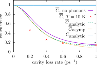
Figure 9: Double-time integrated concurrence $\overline{\overline{C}}$ for a fine structure splitting $\delta=0.1$ meV as a function of the cavity loss rate $\kappa$ without phonons and with phonons at temperature $T$=10 K compared with the analytic result $\overline{\overline{C}}_{\textrm{analytic}}$ for the double-time integrated concurrence without phonons and its asymptotic behavior $\overline{\overline{C}}_{\textrm{asymp}}$. Also shown is the analytic result $C_{\textrm{analytic}}$ for the time-dependent concurrence in the phonon-free case.

Apart from the $\delta$ dependence also the impact of the cavity loss rate $\kappa$ on the different concurrences compared in this paper is instructive. The dependence of the double-time integrated concurrence $\overline{\overline{C}}$ on $\kappa$ is depicted with and without phonons in Fig. 9 for the same fine structure splitting $\delta=0.1$ meV as used in Fig. 5 for the single-time integrated concurrence. While the analytic expression for the time-dependent concurrence $C_{\textrm{anayltic}}$ predicts a value close to one and independent of the loss rate, the double-time integrated concurrence in Fig. 9 significantly depends on $\kappa$ already without phonons: it decreases monotonically with increasing $\kappa$ and follows the asymptotic expression in Eq. (55) for the height of the plateau. The latter is due to the fact that we are considering here a value of $\delta$ where in Fig. 8 already the plateau is reached. While the unnormalized density matrix elements entering the numerator and the denominator in the expression for the single-time integrated concurrence are affected in the same way by a change of $\kappa$, this is not the case for the double-time integrated concurrence. Here, the unnormalized density matrix elements reflect, according to Eq. (50), the competition between two-photon and sequential single-photon processes. The cavity loss rate enters the corresponding contributions in two ways: First, the relative weight of two- and single-photon parts is governed by the ratio of the corresponding emission rates $\kappa_{2P}/\kappa_{1P}=4g^{2}/\kappa^{2}=\tilde{\rho}_{\tilde{G}_{i}\tilde{G}_{j}}(0)/\tilde{\rho}_{\tilde{X}_{i}\tilde{X}_{j}}(0)$. Second, the two-photon parts decay as a function of $\tau$ without oscillations while the sequential single-photon contributions exhibit oscillations reflecting the relative phase between the two involved exciton components. This translates after $\tau$ integration into prefactors $\sim 1/\kappa$ and $\sim 1/[\frac{1}{2}\kappa(\lambda_{i}^{2}+\lambda_{j}^{2})-\frac{i}{\hbar}(E_{\tilde{X}^{\prime}_{i}}-E_{\tilde{X}^{\prime}_{j}})]$. Altogether, in the limit of vanishing $\kappa$ the two-photon contribution dominates irrespective of the other parameters due to the $\sim 1/\kappa^{3}$ singularity and $\overline{\overline{C}}_{\textrm{analytic}}$ approaches $C_{\textrm{analytic}}$ which is close to one. For small enough $\kappa$ and finite $\delta$ the concurrence has reached the plateau with respect to its $\delta$ dependence and is thus well described by Eq. (55), indicating a drop with rising $\kappa$ following a Lorentzian with a FWHM $4g$. We note in passing that when $\kappa$ is further increased for fixed other parameters the width of the peak in Fig. 8 grows $\sim\kappa$ such that according to Eq. (54) $\overline{\overline{C}}_{\textrm{analytic}}$ recovers again to the high value $C_{\textrm{analytic}}$ in the limit $\kappa\to\infty$. However, for the parameters used in Fig. 9 this recovery occurs for much larger $\kappa$ values than covered in the plot.

For $\overline{C}$ as well as $\overline{\overline{C}}$ the interaction with phonons leads to a reduction of the concurrence due to decoherence and because phonons cause the system to be in a mixed state. As discussed before, the phonon impact decreases with increasing cavity loss rate because higher $\kappa$ values limit the time-window over which the phonon-induced decoherence can take place. For the double-time integrated concurrence this is nicely seen in Fig. 9 where the results with and without phonons approach each other for large $\kappa$. Altogether we find a diminishing phonon influence for rising $\kappa$ on top of a nearly constant behavior of the single-time integrated concurrence, while for the double-time integrated concurrence this is superimposed on a strong decay. The resulting total effect is a complete trend reversal for finite $\delta$ in the presence of phonons: $\overline{C}$ increases with rising $\kappa$ while $\overline{\overline{C}}$ decreases as long as $\delta$ is large enough to be in the plateau in Fig. 8.

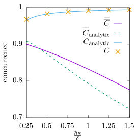
Figure 10: Single- and double-time integrated concurrences for the phonon-free case plotted vs. $\frac{\hbar\kappa}{\delta}$ for fixed $\hbar\kappa\,\delta=0.01$ meV². Shown are the numerically obtained results together with the corresponding analytic approximations.

Interestingly, while the trend reversal as a function of the cavity loss rate is attributed to the phonon influence, the non-equivalence of $\overline{C}$ and $\overline{\overline{C}}$ can already be demonstrated in the phonon-free case. To this end, we plot $\overline{C}$ and $\overline{\overline{C}}$ as a function of $\frac{\hbar\kappa}{\delta}$ for fixed $\hbar\kappa\,\delta$ in Fig. 10. While $\overline{C}$ is increasing monotonically with rising $\frac{\hbar\kappa}{\delta}$, $\overline{\overline{C}}$ is decreasing. The observation of opposite trends in the single- and double-time integrated concurrences has important implications for the interpretation of the results. When comparing different situations, e.g., cavities with different values $\kappa_{1}$ and $\kappa_{2}$, it may turn out that according to $\overline{C}$ the cavity with $\kappa_{1}$ gives rise to the higher entanglement while for $\overline{\overline{C}}$ $\kappa_{2}$ leads to the higher entanglement or vice versa. This clearly demonstrates that $\overline{C}$ and $\overline{\overline{C}}$ cannot be equivalent measures for the same physical quantity, but instead measure two different types of entanglement.

V Conclusion

We have studied the two-photon state generated by the biexciton cascade in a quantum dot embedded in a microcavity. Our main focus is a comparison of dependencies of three different practical definitions of concurrences prevalent in the literature on relevant parameters such as the exciton fine structure splitting and the cavity loss rate. In particular, we compare the time-dependent concurrence $C(t)$ associated with the state of the system at a given time $t$, which by definition reflects the corresponding entanglement of formation, with concurrences derived from the results of different quantum state reconstruction strategies. These strategies are based on photon coincidence measurements collecting data points either over extended real- and delay-time intervals (double-time integrated concurrence $\overline{\overline{C}}$) or over an extended real-time interval but a narrow delay-time window (single-time integrated concurrence $\overline{C}$). Considering the photons recorded in the two detectors of the coincidence measurements, these concurrences refer to photons with a simultaneous emission time $t$ ($C(t)$), photons resulting from simultaneous emission irrespective of the time $t$ of the emission ($\overline{C}$), and photons resulting from emissions without resolving the emission times of both photons ($\overline{\overline{C}}$).

For a quantum dot with finite biexciton binding energy ($E_{B}\gg\delta$) in a cavity whose modes are tuned in resonance with the two-photon transition between the ground and the biexciton state, we have derived analytic expressions for the time-dependent, the single-time integrated, and the double-time integrated concurrence in the absence of dot-phonon interaction. Our results are applicable also beyond the weak-coupling limit of the dot-cavity system and we have shown that they agree well with the results obtained from numerical calculations.

The single-time integrated concurrence, which can be accessed experimentally by time-windowing techniquesStevenson et al. (2008) or using vary narrow time bins for the delay timeBounouar et al. (2018), is found to be close to the stationary value of the time-dependent concurrence at long times. This remains true when the dot-phonon interaction is fully taken into account. The reason for this agreement between $\overline{C}$ and $C(t)$ is that, due to the high energetic penalty involved in the occupation of single-exciton states with one cavity photon, the dynamics of the biexciton cascade is essentially incoherent and exponential, even when the coupling $g$ is comparable to the cavity loss rate $\kappa$. Because all oscillations between the states with two photons in either the horizontally or the vertically polarized cavity mode are overdamped, the time-integration does not lead to a significant dephasing of coherences between those states. Thus, in the dot-cavity configuration considered here, the information contained in $C(t)$ about the entanglement of formation assigned to two-photon states in the cavity at time $t$ is accessible by the more easily measurable single-time integrated concurrence $\overline{C}$.

In contrast, the double-time integrated concurrence, which in most experiments is the measured quantity since measuring over extended real-time and delay-time intervals provides the highest photon coincidence counts, shows a completely different behavior than either $C(t)$ or $\overline{C}$. First of all, disregarding phonons, $\overline{\overline{C}}$ as a function of the fine structure splitting $\delta$ has a narrow peak with a FWHM of approximately $10$ µeV and then drops to a plateau that only weakly depends on the value of the splitting. We also obtain analytic expressions for the height of the plateau as well as the FWHM of the central peak and thereby explain the shape of the double-time integrated concurrence as a function of $\delta$. Numerical simulations reveal that phonons do not change this behavior qualitatively and only lead to quantitative corrections, which is in line with previous studiesHeinze et al. (2017). In contrast, neither with nor without phonons the time-dependent concurrence exhibits a narrow peak as a function of the fine structure splitting which evolves into a plateau for larger splittings. In the phonon-free case it stays close to one even for splittings as large as $\sim 0.1$ meV, while phonons lead to a reduction that follows a bell-shaped curve. This different behavior upon variation of the fine structure splitting can be attributed to the fact that, even in the presence of a non-vanishing fine structure splitting, the two emitted photons are strongly entangled at any given time, which is reflected in the time-dependent and the single-time integrated concurrence. However, the integration over the delay time in the double-time integrated concurrence gives rise to destructive interference of the two pathways.

Another qualitative difference between the time-dependent concurrence and the double-time integrated concurrence is the dependence on the cavity loss rate: The analytic expression for $\overline{C}$, which does not account for the effects of phonons, is independent of the cavity loss rate. Taking dot–LA-phonon interactions into account using a numerically exact real-time path-integral method Cygorek et al. (2017) reveals that phonons can lead to a reduction of the concurrence and that the concurrence increases with the cavity loss rate. The reason for this is that the losses limit the time available for dephasing processes, so that for large $\kappa$ the phonon-induced reduction of the concurrence is suppressed. In contrast, for the considered situation $\overline{\overline{C}}$ decreases with increasing loss rate in the phonon-free case as well as when phonons are taken into account. This $\kappa$ dependence of $\overline{\overline{C}}$ essentially reflects the competition between two- and single-photon processes.

From these results it clearly follows that upon variation of the cavity loss rate opposite orderings are obtained with respect to the two figures of merit provided by $\overline{C}$ and $\overline{\overline{C}}$, respectively. In addition, already in the phonon-free case it turns out that $\overline{C}$ and $\overline{\overline{C}}$ exhibit opposite trends when varying the ratio between $\kappa$ and $\delta$ while keeping the product of these quantities constant. Altogether, this implies that single- and double-time integrated concurrences cannot be equivalent measures for the same physical quantity but instead reflect different aspects of entanglement.

Appendix A Dynamics in the effective three-level system

Here, we calculate the dynamics in the weakly coupled three-level system spanned by the states $|G^{\prime}_{H}\rangle,|G^{\prime}_{V}\rangle$ and $|B^{\prime}\rangle$ defined in Eqs. (30). To this end, we define the density matrix elements

$$\rho_{\nu^{\prime}\mu^{\prime}}:=\langle\big{(}|\nu^{\prime}\rangle\langle\mu^{\prime}|\big{)}\rangle,$$ (58)

with $\nu^{\prime},\mu^{\prime}\in\{G^{\prime}_{H},G^{\prime}_{V},B^{\prime}\}$.

In the subspace spanned by the above states, the Lindblad losses induce transitions to states with lower excitation numbers. However, these states can be disregarded in the equation of motion for $\rho_{\nu^{\prime}\mu^{\prime}}$ since they do not couple back to states with higher excitation numbers. Thus, the trace of the density matrix $\rho$ in the subspace spanned by $\{G^{\prime}_{H},G^{\prime}_{V},B^{\prime}\}$ is no longer conserved and we find

$$\frac{\partial}{\partial t}\rho_{\nu^{\prime}\mu^{\prime}}= \frac{i}{\hbar}\sum_{\bar{\nu}}[H^{\prime}_{\nu^{\prime}\bar{\nu}}\rho_{\bar{\nu}\mu^{\prime}}-\rho_{\nu^{\prime}\bar{\nu}}H^{\prime}_{\bar{\nu}\mu^{\prime}}]$$

$$-\frac{\kappa}{2}\sum_{\bar{\nu}}(n_{\nu^{\prime}\bar{\nu}}\rho_{\bar{\nu}\mu^{\prime}}+\rho_{\nu^{\prime}\bar{\nu}}n_{\bar{\nu}\mu^{\prime}}),$$ (59)

where $n_{\nu^{\prime}\mu^{\prime}}=\sum_{i=H,V}(a^{\dagger}_{i}a_{i})_{\nu^{\prime}\mu^{\prime}}$ is the photon number operator. The equations of motion for the effective three-level system are then

$$\frac{\partial}{\partial t}\rho_{B^{\prime}B^{\prime}}= -(\lambda_{H}^{2}+\lambda_{V}^{2})\kappa\rho_{B^{\prime}B^{\prime}}-\!\!\!\sum_{i\in\{H,V\}}\!\!\!2\tilde{g}_{i}\textrm{Im}(\rho_{G^{\prime}_{i}B^{\prime}}),$$ (60a)

$$\frac{\partial}{\partial t}\rho_{G^{\prime}_{i}B^{\prime}}= \Big{(}i\frac{\tilde{\delta}_{i}}{\hbar}-\kappa\Big{)}\rho_{G^{\prime}_{i}B^{\prime}}+i\tilde{g}_{i}\rho_{B^{\prime}B^{\prime}}-\!\!\!\sum_{j\in\{H,V\}}\!\!\!i\tilde{g}_{j}\rho_{G^{\prime}_{i}G^{\prime}_{j}},$$ (60b)

$$\frac{\partial}{\partial t}\rho_{G^{\prime}_{i}G^{\prime}_{j}}= \Big{[}i\Big{(}\frac{\tilde{\delta}_{i}}{\hbar}-\frac{\tilde{\delta}_{j}}{\hbar}\Big{)}-2\Big{(}1-\frac{1}{2}(\lambda_{i}^{2}+\lambda_{j}^{2})\Big{)}\kappa\Big{]}\rho_{G^{\prime}_{i}G^{\prime}_{j}}$$

$$+i\tilde{g}_{i}\rho_{B^{\prime}G^{\prime}_{j}}-i\tilde{g}_{j}\rho_{G^{\prime}_{i}B^{\prime}},$$ (60c)

where we have defined $\tilde{\delta}_{H/V}=\pm\tilde{\delta}$. It is straightforward to see that when the system is initially in the biexciton state, $\rho_{G^{\prime}_{i}B^{\prime}}=\mathcal{O}(\lambda)$ and $\rho_{G^{\prime}_{i}G^{\prime}_{j}}=\mathcal{O}(\lambda^{2})$. Furthermore, we consider the weak-coupling regime in the effective three-level system where $\tilde{g}_{i}\ll\kappa$. Therefore, $\rho_{G^{\prime}_{i}G^{\prime}_{j}}$ decays fast compared to $\rho_{B^{\prime}B^{\prime}}$ due to the losses and can be neglected for the calculation of $\rho_{G^{\prime}_{i}B^{\prime}}$. Then, the coherences $\rho_{G^{\prime}_{i}B^{\prime}}$ are given by

$$\rho_{G^{\prime}_{i}B^{\prime}}(t)=i\tilde{g}_{i}\int\limits_{0}^{t}dt^{\prime}\,e^{(-\kappa+i\tilde{\delta}_{i}/\hbar)(t-t^{\prime})}\rho_{B^{\prime}B^{\prime}}(t^{\prime}).$$ (61)

Because $\rho_{B^{\prime}B^{\prime}}$ changes only on a much longer time scale (all terms on the r.h.s. of Eq. (60a) are of the order $\mathcal{O}(\lambda^{2})$) than $\rho_{G^{\prime}_{i}B^{\prime}}$, one can apply the Markov limit consisting of evaluating $\rho_{B^{\prime}B^{\prime}}(t^{\prime})$ at $t^{\prime}=t$ and setting the lower limit of the intergral to $-\infty$, so that

$$\rho_{G^{\prime}_{i}B^{\prime}}(t)\approx i\frac{\tilde{g}_{i}}{\kappa-\frac{i}{\hbar}\tilde{\delta}_{i}}\rho_{B^{\prime}B^{\prime}}(t).$$ (62)

Feeding this result back into the equation for $\rho_{B^{\prime}B^{\prime}}$ and dropping terms higher than second order in $\lambda$, one finds

$$\rho_{B^{\prime}B^{\prime}}(t)\approx e^{-\kappa_{B}t},$$ (63)

$$\kappa_{B}\approx(\lambda_{H}^{2}+\lambda_{V}^{2})\Big{(}\frac{4g^{2}}{\kappa}+\kappa\Big{)}.$$ (64)

Using again Eq. (62) one obtains explicit expressions for $\rho_{G^{\prime}_{i}B^{\prime}}$ and its complex conjugate $\rho_{B^{\prime}G^{\prime}_{i}}=(\rho_{G^{\prime}_{i}B^{\prime}})^{*}$, which are the source terms necessary for the calculation of $\rho_{G^{\prime}_{i}G^{\prime}_{j}}$ from Eq.(60):

$$\rho_{G^{\prime}_{i}G^{\prime}_{j}}(t)= \left(\frac{\tilde{g}_{i}\tilde{g}_{j}}{\kappa+\frac{i}{\hbar}\tilde{\delta}_{j}}+\frac{\tilde{g}_{i}\tilde{g}_{j}}{\kappa-\frac{i}{\hbar}\tilde{\delta}_{i}}\right)$$

$$\times\int\limits_{0}^{t}dt^{\prime}\,e^{[-(2-\lambda_{i}^{2}-\lambda_{j}^{2})\kappa+i(\tilde{\delta}_{i}-\tilde{\delta}_{j})/\hbar](t-t^{\prime})}e^{-\kappa_{B}t^{\prime}}.$$ (65)

Integrating over $t^{\prime}$ and keeping only terms up to second order in the prefactor yields

$$\rho_{G^{\prime}_{i}G^{\prime}_{j}}=\frac{\tilde{g}_{i}\tilde{g}_{j}}{\kappa^{2}}\Big{(}e^{-\kappa_{B}t}-e^{[-(2-\lambda_{i}^{2}-\lambda_{j}^{2})\kappa+i(\tilde{\delta}_{i}-\tilde{\delta}_{j})/\hbar]t}\Big{)}.$$ (66)

References

- Gisin et al. (2002) N. Gisin, G. Ribordy, W. Tittel, and H. Zbinden, Rev. Mod. Phys. 74, 145 (2002).
- O’Brian et al. (2009) J. L. O’Brian, A. Furusawa, and J. Vučković, Nature Photonics 3, 687 (2009).
- Orieux et al. (2017) A. Orieux, M. A. M. Versteegh, K. D. Jöns, and S. Ducci, Reports on Progress in Physics 80, 076001 (2017).
- Zeilinger (2017) A. Zeilinger, Physica Scripta 92, 072501 (2017).
- Versteegh et al. (2014) M. A. M. Versteegh, M. E. Reimer, K. D. Jöns, D. Dalacu, P. J. Poole, A. Gulinatti, A. Guidice, and V. Zwiller, Nat. Commun. 5, 5298 (2014).
- Müller et al. (2014) M. Müller, S. Bounouar, K. D. Jöns, M. Glässl, and P. Michler, Nat. Photon. 8, 224 (2014).
- Akopian et al. (2006) N. Akopian, N. H. Lindner, E. Poem, Y. Berlatzky, J. Avron, D. Gershoni, B. D. Gerardot, and P. M. Petroff, Phys. Rev. Lett. 96, 130501 (2006).
- Stevenson et al. (2006) R. M. Stevenson, R. J. Young, P. Atkinson, K. Cooper, D. A. Ritchie, and A. J. Shields, Nature 439, 179 (2006).
- Hudson et al. (2007) A. J. Hudson, R. M. Stevenson, A. J. Bennett, R. J. Young, C. A. Nicoll, P. Atkinson, K. Cooper, D. A. Ritchie, and A. J. Shields, Phys. Rev. Lett. 99, 266802 (2007).
- Hafenbrak et al. (2007) R. Hafenbrak, S. M. Ulrich, P. Michler, L. Wang, A. Rastelli, and O. G. Schmidt, New Journal of Physics 9, 315 (2007).
- Stevenson et al. (2008) R. M. Stevenson, A. J. Hudson, A. J. Bennett, R. J. Young, C. A. Nicoll, D. A. Ritchie, and A. J. Shields, Phys. Rev. Lett. 101, 170501 (2008).
- Bounouar et al. (2018) S. Bounouar, C. de la Haye, M. Strauß, P. Schnauber, A. Thoma, M. Gschrey, J.-H. Schulze, A. Strittmatter, S. Rodt, and S. Reitzenstein, Applied Physics Letters 112, 153107 (2018).
- Pfanner et al. (2008) G. Pfanner, M. Seliger, and U. Hohenester, Phys. Rev. B 78, 195410 (2008).
- Sánchez Muñoz et al. (2015) C. Sánchez Muñoz, F. P. Laussy, C. Tejedor, and E. del Valle, New Journal of Physics 17, 123021 (2015).
- Mar et al. (2016) J. D. Mar, J. J. Baumberg, X. L. Xu, A. C. Irvine, and D. A. Williams, Phys. Rev. B 93, 045316 (2016).
- Bennett et al. (2010) A. J. Bennett, M. A. Pooley, R. M. Stevenson, M. B. Ward, R. B. Patel, A. Boyer de la Giroday, N. Sköld, I. Farrer, C. A. Nicoll, D. A. Ritchie, and A. J. Shields, Nature Physics 6, 947 (2010).
- Seidl et al. (2006) S. Seidl, M. Kroner, A. Högele, K. Karrai, R. J. Warburton, A. Badolato, and P. M. Petroff, Applied Physics Letters 88, 203113 (2006).
- Huber et al. (2014) T. Huber, A. Predojević, M. Khoshnegar, D. Dalacu, P. J. Poole, H. Mejedi, and G. Weihs, Nano Lett. 14, 7107 (2014).
- del Valle et al. (2011) E. del Valle, A. Gonzalez-Tudela, E. Cancellieri, F. P. Laussy, and C. Tejedor, New Journal of Physics 13, 113014 (2011).
- Schumacher et al. (2012) S. Schumacher, J. Förstner, A. Zrenner, M. Florian, C. Gies, P. Gartner, and F. Jahnke, Opt. Express 20, 5335 (2012).
- Liao et al. (2018) S.-K. Liao, W.-Q. Cai, J. Handsteiner, B. Liu, J. Yin, L. Zhang, D. Rauch, M. Fink, J.-G. Ren, W.-Y. Liu, Y. Li, Q. Shen, Y. Cao, F.-Z. Li, J.-F. Wang, Y.-M. Huang, L. Deng, T. Xi, L. Ma, T. Hu, L. Li, N.-L. Liu, F. Koidl, P. Wang, Y.-A. Chen, X.-B. Wang, M. Steindorfer, G. Kirchner, C.-Y. Lu, R. Shu, R. Ursin, T. Scheidl, C.-Z. Peng, J.-Y. Wang, A. Zeilinger, and J.-W. Pan, Phys. Rev. Lett. 120, 030501 (2018).
- Bennett et al. (1996) C. H. Bennett, D. P. DiVincenzo, J. A. Smolin, and W. K. Wootters, Phys. Rev. A 54, 3824 (1996).
- Nielsen and Chuang (2000) M. A. Nielsen and I. L. Chuang, Quantum Computation and Quantum Information (Cambridge University Press, Cambridge, 2000).
- Wootters (2001) W. K. Wootters, Quantum Info. Comput. 1, 27 (2001).
- Wootters (1998) W. K. Wootters, Phys. Rev. Lett. 80, 2245 (1998).
- Hein et al. (2014) S. M. Hein, F. Schulze, A. Carmele, and A. Knorr, Phys. Rev. Lett. 113, 027401 (2014).
- James et al. (2001) D. F. V. James, P. G. Kwiat, W. J. Munro, and A. G. White, Phys. Rev. A 64, 052312 (2001).
- Troiani et al. (2006) F. Troiani, J. I. Perea, and C. Tejedor, Phys. Rev. B 74, 235310 (2006).
- Heinze et al. (2017) D. Heinze, A. Zrenner, and S. Schumacher, Phys. Rev. B 95, 245306 (2017).
- Carmele and Knorr (2011) A. Carmele and A. Knorr, Phys. Rev. B 84, 075328 (2011).
- del Valle (2013) E. del Valle, New Journal of Physics 15, 025019 (2013).
- Reithmaier et al. (2004) J. P. Reithmaier, G. Sęk, A. Löffler, C. Hofmann, S. Kuhn, S. Reitzenstein, L. V. Keldysh, V. D. Kulakovskii, T. L. Reinecke, and A. Forchel, Nature 432, 197 (2004).
- Kuhn et al. (2016) S. C. Kuhn, A. Knorr, S. Reitzenstein, and M. Richter, Opt. Express 24, 25446 (2016).
- Schneider et al. (2016) C. Schneider, P. Gold, S. Reitzenstein, S. Höfling, and M. Kamp, Applied Physics B 122, 19 (2016).
- Reithmaier (2008) J. P. Reithmaier, Semicond. Sci. Technol. 23, 123001 (2008).
- Kasprzak et al. (2013) J. Kasprzak, K. Sivalertporn, F. Albert, C. Schneider, S. Höfling, M. Kamp, A. Forchel, S. Reitzenstein, E. A. Muljarov, and W. Langbein, New Journal of Physics 15, 045013 (2013).
- Winkler (2003) R. Winkler, Spin-Orbit Coupling Effects in Two-Dimensional Electron and Hole Systems, Springer Tracts in Modern Physics, Vol. 191 (Springer, 2003).
- Bravyi et al. (2011) S. Bravyi, D. P. DiVincenzo, and D. Loss, Annals of Physics 326, 2793 (2011).
- Makri and Makarov (1995) N. Makri and D. E. Makarov, The Journal of Chemical Physics 102, 4600 (1995).
- Vagov et al. (2011) A. Vagov, M. D. Croitoru, M. Glässl, V. M. Axt, and T. Kuhn, Phys. Rev. B 83, 094303 (2011).
- Barth et al. (2016) A. M. Barth, A. Vagov, and V. M. Axt, Phys. Rev. B 94, 125439 (2016).
- Cygorek et al. (2017) M. Cygorek, A. M. Barth, F. Ungar, A. Vagov, and V. M. Axt, Phys. Rev. B (Rapid Communication) 96, 201201(R) (2017).
- Glässl et al. (2013) M. Glässl, A. M. Barth, and V. M. Axt, Phys. Rev. Lett. 110, 147401 (2013).
- Nazir and McCutcheon (2016) A. Nazir and D. P. S. McCutcheon, Journal of Physics: Condensed Matter 28, 103002 (2016).