Multiplicative Coevolution Regression Models for Longitudinal Networks and Nodal Attributes

Abstract

We introduce a simple and extendable coevolution model for the analysis of longitudinal network and nodal attribute data. The model features parameters that describe three phenomena: homophily, contagion and autocorrelation of the network and nodal attribute process. Homophily here describes how changes to the network may be associated with between-node similarities in terms of their nodal attributes. Contagion refers to how node-level attributes may change depending on the network. The model we present is based upon a pair of intertwined autoregressive processes. We obtain least-squares parameter estimates for continuous-valued fully-observed network and attribute data. We also provide methods for Bayesian inference in several other cases, including ordinal network and attribute data, and models involving latent nodal attributes. These model extensions are applied to an analysis of international relations data and to data from a study of teen delinquency and friendship networks.

Keywords. vector autoregression, Bayesian inference, binary regression, dynamic data, factor model, probit model, relational data.

1 Introduction

Modern studies of social networks often involve longitudinal measurements over time. Such data can be represented as a sequence of sociomatrices ${\mathbf{Y}}_{0},\ldots,{\mathbf{Y}}_{n}$, where each ${\mathbf{Y}}_{t}$ is a square $m\times m$ matrix with entry $y_{ij,t}$ representing the value of a relationship between nodes $i$ and $j$ at time $t$ (the diagonal entries are typically undefined). Several methods for the analysis of such data have been developed: Important early work in this area has involved stochastic actor-oriented models (Snijders, 2005; Snijders et al., 2010). This approach is based on an economic model of rational choice, whereby individuals make unilateral changes to their networks in order to maximize personal utility functions. Other methods for dynamic network analysis have evolved out of earlier methods for static network data. For example, methods based on temporal exponential random graph models (TERGM) have been developed based on the popular static exponential random graph modeling framework (ERGM) (Hunter et al., 2008; Krivitsky and Handcock, 2014). An alternative approach to static network modeling is one where network patterns are represented with node-specific latent variables (Nowicki and Snijders, 2001; Hoff et al., 2002). Dynamic versions of these models have been developed in Sarkar and Moore (2005); Xing et al. (2010); Ward et al. (2013); Durante and Dunson (2014); Sewell and Chen (2015), among others.

Longitudinal network data will often be accompanied by longitudinal node-level attributes ${\mathbf{X}}_{0},\ldots,{\mathbf{X}}_{n}$, where each ${\mathbf{X}}_{t}$ is an $m\times p$ matrix whose $i$th row is a vector ${\mathbf{x}}_{i,t}$ of characteristics of node $i$ at time $t$. In such cases, it is often of interest to infer how the network and nodal attributes might influence each other over time. To this end, statistical methodology and software have been developed that extends the actor-oriented approach described above (Snijders et al. (2007), http://www.stats.ox.ac.uk/~snijders/siena/). While this work has been groundbreaking, the applicability of an actor-oriented model may be limited to certain types of networks and individual-level characteristics. As described by the primary developers of this approach (Snijders et al., 2007), such a model may not be appropriate in situations where network and behavioral data depend on unobserved latent variables. Such a situation may be present in the study of social networks and obesity: An individual’s body mass index may be related to their social network, but this relationship is likely mediated by other variables such as socioeconomic status, diet, exercise, participation in sports and other variables that may potentially be unobserved. Furthermore, parameter estimation for such actor oriented models is computationally intensive, involving an iterative optimization scheme that requires simulation of hypothetical networks at each iteration.

As an alternative to this actor-oriented approach, in this article we develop a class of coevolution models for network and nodal attribute data that are based on simple and scalable linear regression and latent factor models. Like regression modeling, the framework we present is flexible and extendable, and can be modified to accommodate continuous and ordinal measurements for both the nodal and network data. The framework is built upon a simple autoregressive model that describes the association of both the network ${\mathbf{Y}}_{t}$ and the nodal attributes ${\mathbf{X}}_{t}$ at time $t$ with the values $\{{\mathbf{Y}}_{t-1},{\mathbf{X}}_{t-1}\}$ from the previous time point. The associations are modeled in terms of products of the network and nodal outcomes, and so we refer to such models as multiplicative coevolution regression (MCR) models.

As we discuss in the next section, the parameters of MCR models can quantify three important data features: First, that both the network and nodal attributes may vary smoothly from time point to time point; second, the relations between individuals may be influenced by the similarity of their attributes; and third, individuals may change their attributes based upon the attributes of those with whom they relate. We refer to these three features as autocorrelation, homophily, and contagion, respectively. While the basic MCR model may simply be represented as a type of regression model, in Section 2 we discuss extensions of this model to accommodate network and nodal data that may be binary or ordinal, as well as extensions for data where certain types of network patterns may be well-represented with latent nodal factors. In Section 3 we discuss estimation and inference, including maximum likelihood estimates for fully observed continuous data, and Bayesian inference for a variety of model extensions. In Section 4 we present two case studies. The first involves monthly interactions between 50 countries over a 10 year period. The second analyzes the coevolution of friendship ties and an ordinal measure of delinquency for 26 high-school students. A discussion follows in Section 5.

2 Multiplicative Coevolution Regression

A coevolution model for dynamic network and nodal attribute data should be able to quantify autocorrelation, homophily and contagion. Autocorrelation quantifies the tendency for relations and attributes to vary gradually over time. Homophily refers to the possibility that changes to the relations between nodes may be partly determined by how similar their attributes are. Contagion describes how nodes may change their attributes based on the attributes of those with whom they have relations. For the case of undirected relational data, we propose the following simple multiplicative regression model for describing these three phenomena:

$$y_{ij,t+1} =\mu_{ij}+\alpha y_{ij,t}+{\mathbf{x}}_{i,t}^{T}{\mathbf{H}}{\mathbf{x}}_{j,t}+\epsilon_{ij,t+1},$$ (1)

$${\mathbf{x}}_{i,t+1} ={\boldsymbol{\theta}}_{i}+{\mathbf{A}}{\mathbf{x}}_{i,t}+{\mathbf{C}}{\mathbf{X}}_{t}^{T}{\mathbf{y}}_{i\cdot,t}+{\mathbf{e}}_{i,t+1},$$

where ${\mathbf{y}}_{i\cdot,t}$ is the $i$th row ${\mathbf{Y}}_{t}$ (with $y_{ii,t}=0$), the $\epsilon_{ij,t}$’s are i.i.d. $N(0,\sigma^{2})$ and the ${\mathbf{e}}_{i,t}$’s are i.i.d. $N({\mathbf{0}},{\boldsymbol{\Sigma}})$. Alternatively, the intercept terms $\mu_{ij}$ and ${\boldsymbol{\theta}}_{i}$ can be replaced with regression terms involving exogenous predictors and possibly depending on time.

The parameters $\{\alpha,{\mathbf{A}}\}$, ${\mathbf{H}}$ and ${\mathbf{C}}$ respectively represent the phenomena of autocorrelation, homophily and contagion described above. To see this, note that if ${\mathbf{H}}$ and ${\mathbf{C}}$ were zero, then the model reduces to two first order autoregressive models, with $\alpha$ and ${\mathbf{A}}$ being the autoregression parameters. Regarding homophily, the matrix ${\mathbf{H}}\in\mathbb{R}^{p\times p}$ represents the influence of the similarity between the characteristics of two nodes on their relations. As a simple example, consider the case where ${\mathbf{H}}=h{\mathbf{I}}$ with $h>0$, and so ${\mathbf{x}}_{i,t}^{T}{\mathbf{H}}{\mathbf{x}}_{j,t}=h{\mathbf{x}}_{i,t}^{T}{\mathbf{x}}_{j,t}$. In this case we have positive homophily, in that the more similar $i$ and $j$ are in terms of their attributes at time $t$, the larger the expected relation between them at the next time point. Finally, the matrix ${\mathbf{C}}$ describes contagion, the effect of nodal attributes at time $t$ on those of a given node $i$ at time $t+1$, weighted by the relations of node $i$. For example, assume for the moment that $y_{ij,t}\in\{0,1\}$. In this case, ${\mathbf{X}}_{t}^{T}{\mathbf{y}}_{i\cdot,t}$ is proportional to the average of the characteristic values of those to whom node $i$ is linked.

Model (1) describes the simplest situation we consider in this article, in which the network and nodal attributes are assumed to be Gaussian and fully observed. We refer to this model as a multiplicative coevolution regression (MCR) model. The model is multiplicative in ${\mathbf{Y}}_{t}$ and ${\mathbf{X}}_{t}$ via the homophily and contagion effects. However, as will be discussed in Section 3, it is linear in the parameters and so can be viewed as a multivariate linear regression model.

The assumption of additive effects and normally distributed outcomes is not appropriate for many network datasets. In particular, many network relations are binary or ordinal, and are possibly asymmetric in that $y_{ij,t}$ is not necessarily equal to $y_{ji,t}$. Furthermore, it is often likely to be the case that some variables that drive network formation are unobserved, and not part of the the dataset. In this case, we may want to augment the model to accommodate latent, unobserved nodal characteristics. We consider extensions of the model in (1) to accommodate each of these situations in the following paragraphs.

Ordinal data:

The relational variable $y_{ij,t}$ in many network datasets is binary, indicating whether or not two nodes have some sort of tie between them, such as friendship or social interaction. In other cases this variable is ordinal, such as when $y_{ij,t}$ is recorded as being negative, neutral or positive, or when $y_{ij,t}$ measures the number or intensity of social interactions between two individuals. While the assumptions of Gaussian noise and additive effects of the MCR model will not generally be appropriate for such data, the model can be used to formulate a probit regression model for general ordinal network relations. This is done by expressing the relations $y_{ij,t}$ as a non-decreasing function of latent relations $z_{ij,t}$ that that do follow the MCR model. Specifically, we assume that $y_{ij,t}=f(z_{ij,t})$ for some non-decreasing function $f$, and that the process $\{({\mathbf{Z}}_{t},{\mathbf{X}}_{t}):t=0,\ldots,n\}$ follows the Gaussian MCR model. The only adjustment to the model is that the error variance $\sigma^{2}$ may be assumed to be 1, as otherwise this scale parameter is not separately identifiable from $f$. Furthermore, if the nodal characteristic process $\{{\mathbf{X}}_{t},t=1,\ldots,n\}$ is not well represented with a normal model then an ordinal probit model can be used here as well. In this case, we model $x_{i,k,t}=g_{k}(w_{i,k,t})$ where $g_{1},\ldots,g_{p}$ are nondecreasing functions and $w_{i,k,t}$ is a latent Gaussian process that determines $x_{i,k,t}$. Letting ${\mathbf{W}}_{t}$ be the $n\times p$ matrix with elements $w_{i,k,t}$, the model is completed by assuming $\{({\mathbf{Z}}_{t},{\mathbf{W}}_{t}):t=0,\ldots,n\}$ follows the MCR model. An example data analysis in which the both the relational and attribute variables are ordinal is presented in Section 4.

Directed relations:

Many network datasets include directed relations where $y_{ij,t}$ is not necessarily equal to $y_{ji,t}$. The natural extension of the multiplicative coevolution model in equation (1) to accommodate directed relations is as follows:

$$y_{ij,t+1} =\mu_{ij}+\alpha_{1}y_{ij,t}+\alpha_{2}y_{ji,t}+{\mathbf{x}}_{i,t}^{T}{\mathbf{H}}{\mathbf{x}}_{j,t}+\epsilon_{ij,t+1},$$ (2)

$${\mathbf{x}}_{i,t+1} ={\boldsymbol{\theta}}_{i}+{\mathbf{A}}{\mathbf{x}}_{i,t}+{\mathbf{C}}_{1}{\mathbf{X}}_{t}^{T}{\mathbf{y}}_{i\cdot,t}+{\mathbf{C}}_{2}{\mathbf{X}}_{t}^{T}{\mathbf{y}}_{\cdot i,t}+{\mathbf{e}}_{i,t+1}.$$

The modifications to the model for the network process are that the homophily parameter ${\mathbf{H}}$ is not necessarily symmetric, and that $y_{ij,t+1}$ may be influenced by $y_{ji,t}$ via the reciprocity parameter $\alpha_{2}$. The model for the attribute process now includes two different contagion parameters ${\mathbf{C}}_{1}$ and ${\mathbf{C}}_{2}$. The former represents the relationship-weighted effect of the nodal characteristics of those to which one sends ties, while the latter represents the effect of those from which one receives ties. An example data analysis using a probit version of this directed MCR model appears in Section 4.

Latent nodal attributes:

When nodal attribute data are either not available or only weakly associated with the network process, it may be useful to add latent nodal attributes to the model. In the case of static network modeling, inclusion of latent nodal attributes can provide identification of clusters of nodes, improved model fit and better out-of-sample predictions of unmeasured relations. The basic framework is to model the relation $y_{ij}$ between nodes $i$ and $j$ as depending on the similarity of latent, unobserved characteristics ${\mathbf{x}}_{i}$ and ${\mathbf{x}}_{j}$. For example, the latent class model of Nowicki and Snijders (2001) is equivalent to letting ${\mathbf{x}}_{i}$ represent a vector indicating membership of node $i$ to one of several latent classes. The latent distance model of Hoff et al. (2002) assumes $y_{ij}$ depends on the Euclidean distance between the latent location vectors ${\mathbf{x}}_{i}$ and ${\mathbf{x}}_{j}$. Hoff (2008) shows how both of these approaches are generalized by a multiplicative approach, in which $y_{ij}$ is modeled as a function of the inner product ${\mathbf{x}}_{i}^{T}{\mathbf{H}}{\mathbf{x}}_{j}$. This suggests that, in the absence of nodal characteristics strongly associated with the network process, we allow ${\mathbf{x}}_{i,t}$ in the MCR model (1) to represent latent, unobserved nodal attributes. In this case, both the parameters of the MCR model in (1) and the latent attribute process $\{{\mathbf{X}}_{t}:t=0,\ldots,n\}$ can be estimated from the data. However, the parameters in the MCR model are not fully identifiable when the nodal attributes are latent. For example, the model is invariant to orthogonal rotations of the ${\mathbf{X}}_{t}$’s, that is, replacement of each ${\mathbf{X}}_{t}$ by ${\mathbf{X}}_{t}{\mathbf{R}}$, where ${\mathbf{R}}$ is a $p\times p$ orthogonal matrix so that ${\mathbf{R}}{\mathbf{R}}^{T}={\mathbf{I}}$. For this reason we simplify the latent MCR model by parameterizing the homophily parameter ${\mathbf{H}}$ as being diagonal, and setting ${\boldsymbol{\Sigma}}$ equal to the $p\times p$ identity matrix. Even so, the model remains invariant to simultaneous permutations of the columns of the ${\mathbf{X}}_{t}$’s. This issue is discussed further in the data analysis example in Section 4.

This latent MCR model is similar to several other models developed for the analysis of longitudinal network data that lack nodal attributes. For example, Ward et al. (2013); Durante and Dunson (2014) and Sewell and Chen (2015) each utilize models where the network ${\mathbf{Y}}_{t}$ at each time point is modeled as a function of nodal latent variables ${\mathbf{X}}_{t}$, which in turn follows a stochastic process. These are hidden Markov models for the observed network process, and can be graphically depicted by the dependence graph in the first panel of Figure 1. Such models essentially only include a homophily parameter, modeling a relation between two nodes as a function of their time-varying latent attributes. In contrast, our latent MCR model (depicted in the second panel of the figure) permits a richer description of the evolution of the network by inclusion of an autocorrelation term for the network, and a contagion parameter that allows for the possibility that nodes may change their nodal attributes depending on their past relations.

Figure 1: Dependence graphs for longitudinal network models. Hidden Markov model (left) and latent MCR model (right).

3 Estimation and Inference

One feature of the MCR model is its simplicity: It can be expressed as a pair of linear regression models. As we show in the next subsection, this permits very easy parameter estimation in the case of a normal model for the observed network and attributes. The linear regression framework also serves as a building block for data analysis in more complicated situations, such as the case of ordinal relational and attribute variables and latent attribute models. As we show in Section 3.2, Bayesian inference in such situations can be obtained using relatively straightforward Gibbs sampling algorithms.

3.1 MLEs for normal models

To see how the network evolution model in Equation 1 can be expressed as a linear regression model, first parameterize $\mu_{ij}$ as $\mu_{ij}={\boldsymbol{\gamma}}^{T}{\mathbf{s}}_{ij}$, where ${\mathbf{s}}_{ij}$ is a vector of observed exogenous covariates and ${\boldsymbol{\gamma}}$ is a vector of unknown parameters. If there are no exogenous covariates then we can take ${\boldsymbol{\gamma}}$ to simply be a vector consisting of the values of $\mu_{ij}$ and ${\mathbf{s}}_{ij}$ to be the appropriate binary vector with a single entry equal to one and the remaining entries equal to zero. Then, note that the term ${\mathbf{x}}_{i,t}^{T}{\mathbf{H}}{\mathbf{x}}_{j,t}$ can be written as ${\mathbf{h}}^{T}{\mathbf{x}}_{ij,t}$, where ${\mathbf{h}}=\text{vech}({\mathbf{H}})$ is the “half vectorization” of the matrix ${\mathbf{H}}$ obtained by concatenating the lower-triangular elements of ${\mathbf{H}}$ (including the diagonal), and ${\mathbf{x}}_{ij,t}=\text{vech}({\mathbf{x}}_{i,t}{\mathbf{x}}_{j,t}^{T}+{\mathbf{x}}_{j,t}{\mathbf{x}}_{i,t}^{T}-\text{diag}({\mathbf{x}}_{i,t}{\mathbf{x}}_{j,t}^{T}))$. For example, if each ${\mathbf{x}}_{i,t}$ is two-dimensional, then ${\mathbf{x}}_{ij,t}=(x_{i,1,t}x_{j,1,t},\,x_{i,1,t}x_{j,2,t}+x_{i,2,t}x_{j,1,t},\,x_{i,2,t}x_{j,2,t})$. We can therefore write the network component of model (1) as

$$y_{ij,t}={\boldsymbol{\beta}}^{T}{\mathbf{w}}_{ij,t}+\epsilon_{ij,t},$$

where ${\boldsymbol{\beta}}=({\boldsymbol{\gamma}},\alpha,{\mathbf{h}})$ and ${\mathbf{w}}_{ij,t}=({\mathbf{s}}_{ij},y_{ij,t-1},{\mathbf{x}}_{ij,t})$. The residual sum of squares can be expressed as

$$\sum_{t}\sum_{i<j}(y_{ij,t}-{\boldsymbol{\beta}}^{T}{\mathbf{w}}_{ij,t})^{2}=\left(\sum_{t}\sum_{i<j}y_{ij,t}^{2}\right)-2{\boldsymbol{\beta}}^{T}{\mathbf{l}}+{\boldsymbol{\beta}}^{T}{\mathbf{Q}}{\boldsymbol{\beta}},$$

where

$${\mathbf{l}} =\sum_{t=1}^{n}\sum_{i<j}{\mathbf{w}}_{ij,t}^{T}y_{ij,t}$$ (3)

$${\mathbf{Q}} =\sum_{t=1}^{n}\sum_{i<j}{\mathbf{w}}_{ij,t}{\mathbf{w}}_{ij,t}^{T}.$$

The maximum likelihood estimate of ${\boldsymbol{\beta}}$ is therefore given by $\hat{{\boldsymbol{\beta}}}={\mathbf{Q}}^{-1}{\mathbf{l}}$.

The attribute evolution model is also a linear regression model. Parameterizing ${\boldsymbol{\theta}}_{i}$ as ${\boldsymbol{\Gamma}}{\mathbf{s}}_{i}$ for an exogenous covariate vector ${\mathbf{s}}_{i}$ and parameter matrix ${\boldsymbol{\Gamma}}$, we have ${\mathbf{x}}_{i,t+1}={\mathbf{B}}{\mathbf{w}}_{i,t+1}+{\mathbf{e}}_{i,t+1}$, where ${\mathbf{B}}$ is the column-wise concatenation of ${\boldsymbol{\Gamma}}$, ${\mathbf{A}}$ and ${\mathbf{C}}$, and ${\mathbf{w}}_{i,t+1}$ is the vector obtained by concatenating the vectors ${\mathbf{s}}_{i}$, ${\mathbf{x}}_{i,t}$ and ${\mathbf{X}}_{t}^{T}{\mathbf{y}}_{i\cdot,t}$. The attribute evolution model can be written in matrix form as

$${\mathbf{X}}_{t+1} ={\mathbf{S}}{\boldsymbol{\Gamma}}^{T}+{\mathbf{X}}_{t}{\mathbf{A}}^{T}+{\mathbf{Y}}_{t}{\mathbf{X}}_{t}{\mathbf{C}}^{T}+{\mathbf{E}}_{t+1}$$

$$={\mathbf{W}}_{t+1}{\mathbf{B}}^{T}+{\mathbf{E}}_{t+1},$$

where the $i$th row of ${\mathbf{W}}_{t+1}$ is the vector ${\mathbf{w}}_{i,t+1}$ defined above. A standard result from multivariate regression is that the MLE of ${\mathbf{B}}$ is given by $\hat{{\mathbf{B}}}={\mathbf{L}}{\mathbf{Q}}^{-1}$, where

$${\mathbf{L}} =\sum_{t=1}^{n}\sum_{i=1}^{m}{\mathbf{x}}_{i,t}{\mathbf{w}}_{i,t}^{T}=\sum_{t=1}^{n}{\mathbf{X}}_{t}^{T}{\mathbf{W}}_{t}$$ (4)

$${\mathbf{Q}} =\sum_{t=1}^{n}\sum_{i=1}^{m}{\mathbf{w}}_{i,t}{\mathbf{w}}_{i,t}^{T}=\sum_{t=1}^{n}{\mathbf{W}}_{t}^{T}{\mathbf{W}}_{t}.$$

Estimation for directed relations proceeds with a few modifications. For estimation of the network process, ${\boldsymbol{\beta}}=({\boldsymbol{\gamma}},\alpha_{1},\alpha_{2},{\mathbf{h}})$ where ${\mathbf{h}}=\text{vec}({\mathbf{H}})$, and ${\mathbf{w}}_{ij,t}=({\mathbf{s}}_{ij},y_{ij,t-1},y_{ji,t-1},{\mathbf{x}}_{j,t}\otimes{\mathbf{x}}_{i,t})$, where “$\otimes$” is the Kronecker product. Additionally, the summation in (3) is replaced by a summation over all ordered pairs $\{(i,j):i\neq j\}$. For estimation of the attribute process, the matrix ${\mathbf{B}}$ is the concatenation of ${\boldsymbol{\Gamma}}$, ${\mathbf{A}}$, ${\mathbf{C}}_{1}$ and ${\mathbf{C}}_{2}$, and ${\mathbf{w}}_{i,t+1}$ is the concatenation of the vectors ${\mathbf{s}}_{i}$, ${\mathbf{x}}_{i,t}$, ${\mathbf{X}}_{t}^{T}{\mathbf{y}}_{i\cdot,t}$ and ${\mathbf{X}}_{t}^{T}{\mathbf{y}}_{\cdot i,t}$.

3.2 Bayesian estimation for model extensions

In cases where nodal attributes are not observed or the network and attribute processes are not plausibly Gaussian, the MCR model will have to be extended as described in Section 2. For these cases we propose a Bayesian approach to inference, as a posterior approximation scheme based on Gibbs sampling is modular and can be easily modified to accommodate different features of the data. We first discuss Bayesian inference for the basic MCR model described in Equation 1, and then discuss two modifications, permitting the modeling of unobserved latent attributes and the modeling of ordinal network and attribute data.

Let ${\boldsymbol{\beta}}=(\gamma,\alpha,{\mathbf{h}})$ and ${\mathbf{B}}=[{\boldsymbol{\Gamma}}\,{\mathbf{A}}\,{\mathbf{C}}]$ be the regression parameters in the network and attribute processes respectively. Using semiconjugate prior distributions for the unknown parameters ${\boldsymbol{\beta}}$, ${\mathbf{B}}$, $\sigma^{2}$ and ${\boldsymbol{\Sigma}}$, their joint posterior distribution can be approximated with a Gibbs sampler that iteratively simulates values of these parameters from their full conditional distributions. Specifically, if the prior distributions are ${\boldsymbol{\beta}}\sim N({\mathbf{0}},{\mathbf{V}}_{\beta})$, ${\mathbf{b}}=\text{vec}({\mathbf{B}})\sim N({\mathbf{0}},{\mathbf{V}}_{\rm b})$, $1/\sigma^{2}\sim$ gamma$(\nu_{0}/2,\nu_{0}\sigma_{0}^{2}/2)$, and ${\boldsymbol{\Sigma}}^{-1}\sim$Wishart$({\mathbf{S}}_{0}^{-1},\eta_{0})$, then the Gibbs sampler proceeds by iterating the following steps:

1. Simulate ${\boldsymbol{\beta}}$ from its multivariate normal full conditional distribution with mean $({\mathbf{V}}_{\beta}^{-1}+{\mathbf{Q}})^{-1}{\mathbf{l}}$ and variance $({\mathbf{V}}_{\beta}^{-1}+{\mathbf{Q}})^{-1}$, where ${\mathbf{Q}}$ and ${\mathbf{l}}$ are as in (3).

2. Simulate ${\mathbf{b}}$ from its multivariate normal full conditional distribution with mean $({\mathbf{V}}_{b}^{-1}+{\mathbf{Q}}\otimes{\boldsymbol{\Sigma}}^{-1})^{-1}\text{vec}({\mathbf{L}})$ and variance $({\mathbf{V}}_{b}^{-1}+{\mathbf{Q}}\otimes{\boldsymbol{\Sigma}}^{-1})^{-1}$, where ${\mathbf{Q}}$ and ${\mathbf{L}}$ are as in (4).

3. Simulate $1/\sigma^{2}\sim$ gamma$([\nu_{0}+nm(m-1)/2]/2,[\nu_{0}\sigma^{2}_{0}+RSS)]/2)$, where

   $$RSS=\sum_{t=1}^{n}\sum_{i<j}(y_{ij,t}-[\mu_{ij}+\alpha y_{ij,t-1}+{\mathbf{x}}_{i,t-1}^{T}{\mathbf{H}}{\mathbf{x}}_{j,t-1}])^{2}.$$

4. Simulate ${\boldsymbol{\Sigma}}^{-1}\sim$ Wishart$([{\mathbf{S}}_{0}+{\bf RSS}]^{-1},\eta_{0}+mn)$, where

   $${\bf RSS}=\sum_{t=1}^{n}({\mathbf{X}}_{t}-[\Theta+{\mathbf{X}}_{t-1}{\mathbf{A}}^{T}+{\mathbf{Y}}_{t-1}{\mathbf{X}}_{t-1}{\mathbf{C}}^{T}])^{T}({\mathbf{X}}_{t}-[\Theta+{\mathbf{X}}_{t-1}{\mathbf{A}}^{T}+{\mathbf{Y}}_{t-1}{\mathbf{X}}_{t-1}{\mathbf{C}}^{T}]).$$

Iteration of this algorithm generates a Markov chain with a stationary distribution equal to the posterior distribution of $({\boldsymbol{\beta}},{\mathbf{b}},\sigma^{2},{\boldsymbol{\Sigma}})$. The empirical distribution of the simulated parameter values can be used to obtain approximate posterior means, quantiles and confidence intervals. Furthermore, the Gibbs sampling algorithm can be modified or extended to provide inference for related models and data structures. We consider two such modifications below.

Latent attribute models:

The Gibbs sampling algorithm may be easily modified to accommodate the case that the ${\mathbf{x}}_{i,t}$’s are estimated latent attributes rather than observed attributes. Recall from the discussion in Section 2 that in this case we fix ${\boldsymbol{\Sigma}}={\mathbf{I}}$ for reasons of identifiability. As such, we replace Step 4 in the Gibbs sampler described above with the following step that iteratively simulates values of the ${\mathbf{x}}_{i,t}$’s from their full conditional distributions:

1. Iteratively over nodes $i=1,\ldots,m$ and time points $t=0,\ldots,n$, simulate ${\mathbf{x}}_{i,t}$ from its multivariate normal full conditional distribution. For a time point $t$ such that $0<t<n$, this full conditional distribution has mean ${\mathbf{Q}}^{-1}{\mathbf{l}}$ and variance ${\mathbf{Q}}^{-1}$, where ${\mathbf{l}}=\sum_{k=1}^{3}{\mathbf{W}}_{k}^{T}{\mathbf{z}}_{k}$ and ${\mathbf{Q}}=\sum_{k=1}^{3}{\mathbf{W}}_{k}^{T}{\mathbf{W}}_{k}$ are given as follows:

   $${\mathbf{W}}_{1}={\mathbf{I}} {\mathbf{z}}_{1}={\boldsymbol{\theta}}_{i}+{\mathbf{A}}{\mathbf{x}}_{i,t-1}+{\mathbf{C}}{\mathbf{X}}_{t-1}^{T}{\mathbf{y}}_{i\cdot,t-1}$$

   $${\mathbf{W}}_{2}=\tilde{{\mathbf{X}}}_{t}{\mathbf{H}}/\sigma {\mathbf{z}}_{2}=(\tilde{{\mathbf{y}}}_{i\cdot,t+1}-\tilde{{\boldsymbol{\mu}}}_{i\cdot}-\alpha\tilde{{\mathbf{y}}}_{i\cdot,t})/\sigma$$

   $${\mathbf{W}}_{3}={\mathbf{e}}_{i}\otimes{\mathbf{A}}+{{\mathbf{y}}_{i\cdot}}_{t}\otimes{\mathbf{C}} {\mathbf{z}}_{3}=\text{vec}({\mathbf{X}}_{t+1}-\Theta-\tilde{{\mathbf{I}}}^{T}\tilde{{\mathbf{X}}}_{t}{\mathbf{A}}^{T}-\tilde{{\mathbf{Y}}}_{t}^{T}\tilde{{\mathbf{X}}}_{t}{\mathbf{C}}^{T}),$$

where ${\mathbf{e}}_{i}$ is a vector of zeros except for a one in the $i$th entry, and the tildes in the formulas for ${\mathbf{W}}_{2},{\mathbf{W}}_{3}$ and ${\mathbf{z}}_{2},{\mathbf{z}}_{3}$ indicate the removal of the $i$th row of a matrix or the $i$th element of a vector. The three terms in the sums for ${\mathbf{l}}$ and ${\mathbf{Q}}$ represent information about ${\mathbf{x}}_{i,t}$ from the past, from the future network, and from the future attributes, respectively. The values of ${\mathbf{x}}_{i,0}$ and ${\mathbf{x}}_{i,n}$ are updated similarly, except in the former case we have ${\mathbf{z}}_{1}={\mathbf{0}}$, and in the latter case we have ${\mathbf{l}}={\mathbf{W}}_{1}^{T}{\mathbf{z}}_{1}$ and ${\mathbf{Q}}={\mathbf{W}}_{1}^{T}{\mathbf{W}}_{1}$. As discussed in Section 2, we also restrict ${\mathbf{H}}$ to be a diagonal matrix when the attributes are latent. As a result, the calculation of ${\mathbf{l}}$ in Step 1 of the Gibbs sampler is as in (3) except that it is computed with ${\mathbf{x}}_{ij,t}=({\mathbf{x}}_{j,t}\circ{\mathbf{x}}_{j,t})$, where “$\circ$” denotes element-wise multiplication. This is because ${\mathbf{x}}_{i,t}^{T}{\mathbf{H}}{\mathbf{x}}_{j,t}=({\mathbf{x}}_{j,t}\circ{\mathbf{x}}_{j,t})^{T}{\mathbf{h}}$ in this case where ${\mathbf{H}}$ is diagonal. A numerical illustration of this Gibbs sampler as applied to longitudinal international relations data is provided in Section 4.1.

Probit models for ordinal outcomes:

Ordinal network and attribute data may be accommodated by modeling the observed network and attribute processes as non-decreasing functions of latent processes that do follow the Gaussian MCR model in Equation 1. Specifically, let $y_{ij,t}$ be the observed ordinal-valued relation between nodes $i$ and $j$ at time $t$, and let $x_{i,k,t}$ be the value of the $k$th ordinal-valued attribute of node $i$ at time $t$. We then model the network and attribute process by assuming $y_{ij,t}=f(z_{ij,t})$ and $x_{i,k,t}=g_{k}(w_{i,k,t})$, where $f$ and $g_{1},\ldots,g_{p}$ are unknown non-decreasing step functions, and the $z_{ij,t}$’s and $w_{i,k,t}$’s follow the Gaussian MCR model. A Gibbs sampler for this probit MCR model may be obtained by adding to Steps 1-4 above a few additional steps to simulate values of the $z_{ij,t}$’s, the $w_{i,k,t}$’s from their full conditional distributions, as well as the values defining $f$ and $g_{1},\ldots,g_{p}$. Such steps are standard in the literature on Bayesian modeling of ordinal data: Assuming normal prior distributions for the locations of the jumps in $f$, $g_{1},\ldots,g_{p}$, the full conditional distributions of all of these quantities are constrained normal distributions, which may be simulated from using the inverse-CDF method. For information on such procedures in general, see Albert and Chib (1993). Details of the Gibbs sampler for the MCR model in particular can be found in Appendix A. An example data analysis using the probit MCR model appears in Section 4.2.

4 Example Data Analyses

In this section we illustrate the use of the MCR model with two example data analyses. The first example applies the model to a time series of international relations between 50 countries over a ten year period using a latent Gaussian MCR model. The second example studies the coevolution of the friendships and delinquency behaviors of 26 high-school students. In this latter example the network is binary and the nodal attribute is ordinal, and so an ordinal MCR model is employed.

4.1 International Relations

The ICEWS project (http://www.lockheedmartin.com/us/products/W-ICEWS/iData.html) gathers data on international events occurring between countries. For this article, we analyze a monthly summary of the undirected dyadic relations between the 50 most active countries in the ICEWS database during a 112 month period from 2006 to 2015. Events between countries are assigned event codes, and each event has an associated intensity score ranging from -10 for extreme negative relations to +10 for extreme positive relations (Boschee et al., 2016). For this analysis, we computed the monthly sum of these intensity scores for each pair of countries, and then applied a normal quantile-quantile transformation to all values. This resulted in a time series of 112 $50\times 50$ sociomatrices ${\mathbf{Y}}_{0},\ldots,{\mathbf{Y}}_{111}$, where $y_{ij,t}$ is the (transformed) intensity score sum between countries $i$ and $j$ for month $t$.

We fit the latent MCR model described in Section 2 with $p=2$ latent attributes for each country at each time point. With all regression coefficients being a priori i.i.d. $N(0,100)$, and $\nu_{0}=\sigma^{2}_{0}=1$, the Gibbs sampler described in Section 3.2 was run for 27,500 iterations. The first 2,500 iterations of the algorithm were dropped to allow for burn-in, and every 10th iteration thereafter was saved, yielding 2,500 simulated values for each parameter with which to approximate the posterior distribution. The average effective sample size across parameters in the MCR model was 789.

A 95% posterior credible interval for $\alpha$ is (0.134,0.145), indicating strong evidence for positive autocorrelation, and the diagonal values of ${\mathbf{H}}$ were positive for every iteration of the Gibbs sampler, indicating positive homophily. To get a sense of the magnitude of these coefficients, we computed the relative sum of squares contributions of the four terms of the network coevolution model, averaged across time points. These contributions were 28.2, 2.3, 16.2 and 53.2 percent, respectively, for the $\mu_{i,j}$’s, the autoregressive term, the homophily term and the error variance, respectively.

quantile	$a_{1,1}$	$a_{1,2}$	$a_{2,1}$	$a_{2,2}$	$c_{1,1}$	$c_{1,2}$	$c_{2,1}$	$c_{2,2}$
2.5%	0.148	0.044	-0.004	0.339	0.005	-0.002	0.001	0.015
50%	0.193	0.094	0.047	0.388	0.006	0.000	0.004	0.018
97.5%	0.241	0.144	0.098	0.438	0.008	0.002	0.006	0.020

Table 1: Posterior quantiles of parameters in the attribute evolution process for the ICEWS data.

Posterior medians and 95% credible intervals for the ${\mathbf{A}}$ and ${\mathbf{C}}$ parameters of the attribute evolution model are given in Table 1. The most significant terms in these two matrices are the diagonal terms, indicating that the two latent attribute processes both show positive autocorrelation and positive contagion, but not strong interdependence with each other. The magnitude of the autocorrelation and contagion effects can be assessed by computing the sum of squares of these terms relative to the ${\boldsymbol{\theta}}_{i}$’s and the error term, averaged across time points. These contributions were 60.0, 9.3, 4.6 and 26.1 percent, respectively, for the ${\boldsymbol{\theta}}_{i}$’s, the autoregressive term, the contagion term and the error variance, respectively.

Figure 2 plots the times series of the estimated latent attributes for a few selected countries. The top panel plots the first attribute (corresponding to the larger of the two homophily effects) for the United States, the United Kingdom and Iran. The plot indicates that this factor contributes positively to the relationship between the United States and the United Kingdom throughout the time period (as the estimated attributes have the same sign), whereas the contribution to the relationships of these countries with Iran is neutral until early 2013, when Hassan Rouhani was elected President over several hardline candidates and indicated a desire to negotiate a nuclear accord. The second panel of the figure plots a time series of the second latent attribute for Ukraine, Germany and Russia. In this plot we see that the time series for Russia and Ukraine are similar until the very beginning of 2014, when the protests against the Russian-backed government of President Yanukovych began.

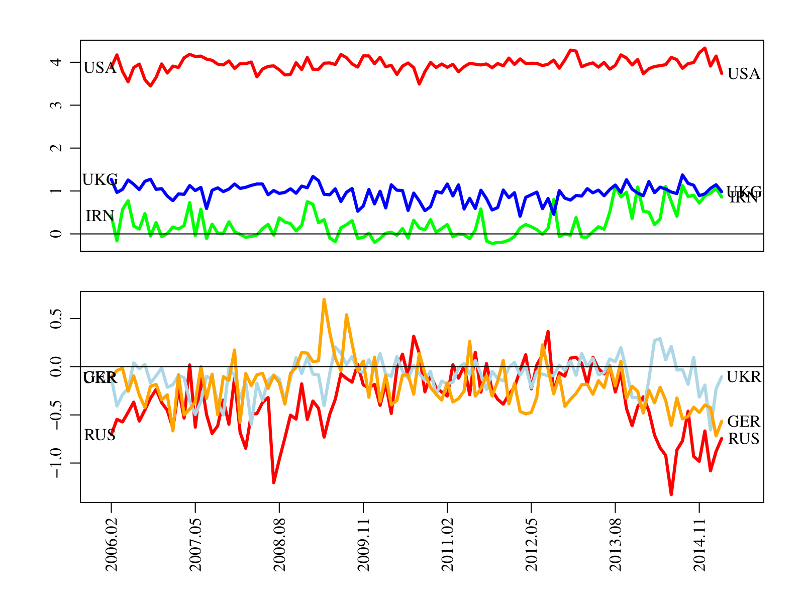
Figure 2: Time series of selected country-specific latent attributes. The top plot gives the estimated values of the first factor for the United States (USA), Iran (IRN) and the United Kingdom (UKG). The lower plot gives values of the second factor for Ukraine (UKR), Germany (GER) and Russia (RUS).

Finally, we performed a small out-of-sample forecasting study to assess the benefit of the proposed model over the type of hidden Markov model considered in Ward et al. (2013); Durante and Dunson (2014), and displayed graphically in the left-hand side of Figure 1. Such models lack the network autocorrelation term $\alpha$ and the contagion term ${\mathbf{C}}$. To assess the predictive benefit of these effects we considered four models - with and without $\alpha$ and with and without ${\mathbf{C}}$. We obtained five one-month-ahead forecasts for each model, using data up to and including months 87, 92, 97, 102, 107 to predict the value of the network at time 88, 93, 98, 103 and 108 respectively. In terms of prediction error sum of squares, the full MCR model with network autocorrelation and contagion effects performed the best for each month forecasted. However, the submodel without contagion effects only performed 1.5% worse, on average over the five months forecasted. However, the submodel lacking both network autocorrelation and contagion performed on average 6.8% worse, suggesting that for these data, network autocorrelation effects are more important than contagion effects for forecasting the network.

4.2 Friendship and Delinquency

Knecht et al. (2007) gathered gathered data on a small directed friendship network of 25 Dutch secondary school students, along with nodal attributes including sex and a five-level ordinal measure of delinquency. Both delinquency and the friendship network were measured at four time points during a year-long period.

We model the coevolution of friendship and delinquency over the study period with an ordinal MCR model. Specifically, we model the binary friendship indicator $y_{ij,t}$ as $y_{ij,t}=f(z_{ij,t})$, and the delinquency category $x_{i,t}$ as $x_{i,t}=g(w_{i,t})$, where $f$ and $g$ are non-decreasing functions and $z_{ij,t}$ and $w_{i,t}$ follow a Gaussian MCR model:

$$z_{ij,t+1} ={\boldsymbol{\beta}}^{T}{\mathbf{s}}_{i,j}+\alpha_{1}z_{ij,t}+\alpha_{2}z_{ji,t}+hw_{i,t}w_{j,t}+\epsilon_{ij,t+1}$$

$$w_{i,t+1} =bs_{i}+aw_{i,t}+c_{1}{\mathbf{w}}_{t}^{T}{\mathbf{z}}_{i\cdot,t}+c_{2}{\mathbf{w}}_{t}^{T}{\mathbf{z}}_{\cdot i,t}+e_{i,t+1}$$

$$\{\epsilon_{i,j,t}\},\{e_{i,t}\} \sim\text{ i.i.d. }N(0,1),$$

where $\alpha_{1}$, $\alpha_{2}$ and $a$ describe network autocorrelation, network reciprocity, and delinquency autocorrelation respectively, $h$ is a homophily parameter and $c_{1}$ and $c_{2}$ are contagion parameters. Additionally, $s_{i}$ is the binary indicator that student $i$ is female, and ${\mathbf{s}}_{i,j}=(s_{i},s_{j},1(s_{i}=s_{j}))$ is a vector describing the gender characteristics of the directed dyad $(i,j)$. The unknown parameters ${\boldsymbol{\beta}}$ and $b$ describe the effects of gender on temporal changes to the network and the nodal attributes, respectively. We also note that the latent variables $z_{i,j,1}$ and $w_{i,1}$ at the first time point were modeled as $z_{i,j,1}\sim N({\boldsymbol{\gamma}}^{T}{\mathbf{s}}_{i,j},\sigma^{2})$ and $w_{i,1}\sim N(gs_{i},\tau^{2})$, respectively. The parameters ${\boldsymbol{\beta}}_{1}$ and $b_{1}$ describe the effects of gender on the initial state of the network and delinquency.

The parameters in this model were estimated using the Gibbs sampler for ordinal data described in Section 3. We ran the MCMC algorithm for 40,000 iterations, and dropped the first 20,000 iterations to allow for burn-in of the Markov chain. The lowest effective sample size among the regression parameters was 643, and the median effective sample size was around 3000. Posterior medians and 95% posterior credible intervals are given in Table 2.

	$\beta_{1}$	$\beta_{2}$	$\beta_{3}$	$\alpha_{1}$	$\alpha_{2}$	$h$	$b$	$a$	$c_{1}$	$c_{2}$
2.5 %	-0.412	-0.205	0.081	0.438	0.286	0.023	-0.219	0.319	-0.061	-0.033
50 %	-0.278	-0.072	0.240	0.530	0.374	0.084	0.269	0.583	-0.001	0.028
97.5 %	-0.145	0.064	0.395	0.621	0.463	0.200	0.778	0.845	0.057	0.090

	$\gamma_{1}$	$\gamma_{2}$	$\gamma_{3}$	$g$
2.5%	-0.399	-0.277	0.662	-1.966
50%	-0.177	-0.060	0.879	-0.864
97.5%	0.027	0.140	1.104	-0.088

Table 2: Posterior quantiles of MCR model parameters for the friendship and delinquency data.

The results indicate evidence of positive autocorrelation for both the network and attribute processes (represented by $\alpha_{1}$, $\alpha_{2}$ and $a$), positive homophily with respect to the delinquency attribute ($h$), but not not evidence of contagion ($c_{1}$ and $c_{2}$). This lack of evidence for contagion is in accord with the results of Snijders et al. (2010), who used a stochastic actor-based utility model to analyze these data. Additionally, the posterior distributions of ${\boldsymbol{\beta}}$ and ${\boldsymbol{\gamma}}$ indicate evidence of homophily with respect to sex, and that males had a higher rate of increase in friendship nominations over time. The posterior distributions of $b$ and $g$ indicated a lower rate of delinquency among females at the beginning of the study ($g$) but not a further effect of sex on the delinquency process ($b$).

5 Discussion

In this paper we developed a multiplicative co-evolution regression (MCR) model for dynamic network and nodal attribute data, which is able to quantify patterns of autoregression, homophily and contagion in social networks. In the simplest case of a Gaussian network outcome and Gaussian attribute data, the model is essentially a vector autoregressive model. For the more typical case that the network or nodal attribute data are binary or ordinal, we developed a Bayesian approach to parameter estimation and inference.

This Bayesian approach permits straightforward extensions to the basic MCR model. For example, latent nodal attributes can be included to explain network patterns that is not well-explained by the observed attributes. In this case, we can also model the co-evolution of the network and the latent nodal attributes.

The work of Snijders et al. (2010) and Hanneke et al. (2010) provide methods for modeling evolution of network based on network statistics including density, stability, reciprocity and transitivity. While the MCR model does not require such terms, such effects can be estimated by including network statistics in the regression model. For example, to estimate reciprocity, we include $y_{ji,t-1}$ as a predictor for $y_{ij,t}$.

Appendix A Gibbs sampler for probit MCR

When $y_{ij,t}$’s are ordinal-valued, we model the network with a probit link and assume $y_{ij,t}=f(z_{ij,t})$. The Gibbs sampler for the probit MCR then include the Steps 1-4 as described in Section 3.2 and also an addition step to update the $z_{ij,t}$’s.

Denote

$$\left\{\begin{split}\mathbf{h}_{i,t+1}^{-j}&\equiv\mathbf{x}_{i,t+1}-\boldsymbol{\theta}_{i}-\mathbf{A}^{T}\mathbf{x}_{i,t}-\mathbf{C}\mathbf{X}_{-j\cdot,t}^{T}{\mathbf{z}_{i,-j,t}},\\ \mathbf{h}_{j,t+1}^{-i}&\equiv\mathbf{x}_{j,t+1}-\boldsymbol{\theta}_{j}^{X}-\mathbf{A}^{T}\mathbf{x}_{j,t}-\mathbf{C}\mathbf{X}_{-i\cdot,t}^{T}{\mathbf{z}_{-i,j,t}},\\ \mathbf{R}_{t}&\equiv\mathbf{M}_{t}+\mathbf{X}_{t}\mathbf{H}\mathbf{X}_{t}^{T},\\ \end{split}\right.$$

where $\mathbf{X}_{-i\cdot,t}$ refers to the sub-matrix of $\mathbf{X}_{t}$ with the $i$-th row removed and $\mathbf{M}_{t}$ refers to the matrix of $\{\mu_{ij}\}$. Then the equations related to $z_{ij,t}$ include

$$\begin{split}z_{ij,t}&=\alpha z_{ij,t-1}+r_{ij,t-1}+\epsilon_{ij,t},\\ z_{ij,t+1}&=\alpha z_{ij,t}+r_{ij,t}+\epsilon_{ij,t+1},\\ \mathbf{h}_{i,t+1}^{-j}&=z_{ij,t}\mathbf{C}\mathbf{x}_{i,t}+\mathbf{e}_{i,t+1},\\ \mathbf{h}_{j,t+1}^{-i}&=z_{ij,t}\mathbf{C}\mathbf{x}_{j,t}+\mathbf{e}_{j,t+1}.\\ \end{split}$$ (5)

Given the prior $z_{ij,t}\sim\rm{N}(\mu_{0},\sigma_{0}^{2})$, the full conditional distribution of $z_{ij,t}$ is given by $\rm{N}(\mu_{ij,t},\sigma_{ij,t}^{2})$, where

$$\begin{split}\sigma_{ij,t}^{2}&=\left(\frac{1+\alpha^{2}}{\sigma^{2}}+\mathbf{x}^{T}_{i,t}\mathbf{C}^{T}\boldsymbol{\Sigma}^{-1}\mathbf{C}\mathbf{x}_{i,t}+\mathbf{x}^{T}_{j,t}\mathbf{C}^{T}\boldsymbol{\Sigma}^{-1}\mathbf{C}\mathbf{x}_{j,t}+\frac{1}{\sigma_{0}^{2}}\right)^{-1},\\ \mu_{ij,t}&=\sigma_{ij,t}^{2}\left(\frac{\alpha z_{ij,t-1}+r_{ij,t-1}+\alpha(z_{ij,t+1}-r_{ij,t})}{\sigma^{2}}+\mathbf{x}^{T}_{i,t}\mathbf{C}^{T}\boldsymbol{\Sigma}^{-1}\mathbf{h}_{i,t+1}^{-j}+\mathbf{x}^{T}_{j,t}\mathbf{C}^{T}\boldsymbol{\Sigma}^{-1}\mathbf{h}_{j,t+1}^{-i}+\frac{\mu_{0}}{\sigma_{0}^{2}}\right).\\ \end{split}$$

However, we cannot directly sample from the full conditional distribution due to the restriction of $y_{ij,t}$. Luckily, we only need to restrict our sampling to the interval $[z_{ij,t}^{-},z_{ij,t}^{+}]$, rather than change the full conditionals. The idea for getting the intervals is that the upper bound cannot exceed the minimum value among all the entries of $\mathbf{Z}$ whose corresponding entries in $\mathbf{Y}$ is higher than $y_{ij,t}$. Similarly, the lower bound is determined by the maximum of those with values in $\mathbf{Y}$ lower than $y_{ij,t}$, i.e.,

$$\left\{\begin{split}z_{ij,t}^{+}&={\rm min}\{z_{kl,s}:y_{kl,s}>y_{ij,t};k,l\in\{1,\cdots,m\},k\neq l,s\in\{1,\cdots,n\},(k,l,s)\neq(i,j,t)\},\\ z_{ij,t}^{-}&={\rm max}\{y_{kl,s}:y_{kl,s}<y_{ij,t};k,l\in\{1,\cdots,m\},k\neq l,s\in\{1,\cdots,n\},(k,l,s)\neq(i,j,t)\}.\\ \end{split}\right.$$

This method is known as rank likelihood, which is introduced in Hoff [2009]. In this book, the author also presents an alternative way that works for ordinal data with ranks $\{1,\cdots,q\}$. Using this method, we need to update the thresholds $\{h_{0},\cdots,h_{q}\}$ during the Gibbs sampler procedure. Assume a prior for all the thresholds and during the iteration, the threshold $h_{s}$ is sampled according to the interval $[h_{s}^{-},h_{s}^{+}]$, where $h_{s}^{+}={\rm min}\{y_{kl,s}:y_{kl,s}=s+1\}$ and $h_{s}^{-}={\rm max}\{y_{kl,s}:y_{kl,s}=s\}$.

To estimate the parameters and latent variables in the model with both ordinal networks and ordinal nodal attributes, we can still follow the Gibbs sampler procedure discussed here, along with an extra step to update $w_{i,k,t}$. In each iteration, we can sample a new point for $w_{i,k,t}$ from its full conditional distribution with restrict to interval $[w_{i,k,t}^{-},w_{i,k,t}^{+}]$. The boundaries/thresholds can be obtained using rank likelihood or sampled from their full conditionals.

References

- Albert and Chib [1993] James H. Albert and Siddhartha Chib. Bayesian analysis of binary and polychotomous response data. J. Amer. Statist. Assoc., 88(422):669–679, 1993. ISSN 0162-1459. URL http://links.jstor.org/sici?sici=0162-1459(199306)88:422<669:BAOBAP>2.0.CO;2-T&origin=MSN.
- Boschee et al. [2016] Elizabeth Boschee, Jennifer Lautenschlager, Sean O’Brien, Steve Shellman, James Starz, and Michael Ward. Icews coded event data, 2016. URL http://dx.doi.org/10.7910/DVN/28075.
- Durante and Dunson [2014] Daniele Durante and David B. Dunson. Bayesian dynamic financial networks with time-varying predictors. Statistics and Probability Letters, 93:19–26, 2014. ISSN 01677152.
- Hanneke et al. [2010] Steve Hanneke, Wenjie Fu, and Eric Xing. Discrete Temporal Models of Social Networks. Electronic Journal of Statistics, 4:585–605, 2010. ISSN 1935-7524. doi: 10.1214/09-EJS548. URL http://arxiv.org/abs/0908.1258.
- Hoff [2008] Peter D. Hoff. Modeling homophily and stochastic equivalence in symmetric relational data. Nips, pages 657–664, 2008. URL http://arxiv.org/abs/0711.1146.
- Hoff [2009] Peter D. Hoff. A First Course in Bayesian Statistical Methods. 2009. doi: 10.1007/978-0-387-92407-61.
- Hoff et al. [2002] Peter D Hoff, Adrian E Raftery, and Mark S Handcock. Latent Space Approaches to Social Network Analysis. Journal of the American Statistical Association, 97(460):1090–1098, 2002. ISSN 0162-1459. doi: 10.1198/016214502388618906.
- Hunter et al. [2008] David R Hunter, Mark S Handcock, Carter T Butts, Steven M Goodreau, and Martina Morris. ergm: A package to fit, simulate and diagnose exponential-family models for networks. Journal of statistical software, 24(3):nihpa54860, 2008.
- Knecht et al. [2007] Stefan Knecht, Julia Reinholz, and Peter Kenning. The spread of obesity in a social network. The New England journal of medicine, 357(18):1866–1867; author reply 1867–1868, 2007. ISSN 0028-4793. doi: 10.1056/NEJMc072478.
- Krivitsky and Handcock [2014] Pavel N. Krivitsky and Mark S. Handcock. A separable model for dynamic networks. J. R. Stat. Soc. Ser. B. Stat. Methodol., 76(1):29–46, 2014. ISSN 1369-7412. doi: 10.1111/rssb.12014. URL http://dx.doi.org/10.1111/rssb.12014.
- Nowicki and Snijders [2001] Krzysztof Nowicki and Tom a. B Snijders. Estimation and Prediction for Stochastic Blockstructures. Journal of the American Statistical Association, 96(455):1077–1087, 2001. ISSN 0162-1459. doi: 10.1198/016214501753208735.
- Sarkar and Moore [2005] Purnamrita Sarkar and Andrew W Moore. Dynamic social network analysis using latent space models. ACM SIGKDD Explorations Newsletter, 7(2):31–40, 2005.
- Sewell and Chen [2015] Daniel K Sewell and Yuguo Chen. Latent Space Models for Dynamic Networks. Journal of the American Statistical Association, (April):37–41, 2015. doi: 10.1080/01621459.2014.988214.
- Snijders et al. [2010] T. a B Snijders, Gerhard G. van de Bunt, and C. E G Steglich. Introduction to stochastic actor-based models for network dynamics. Social Networks, 32(1):44–60, 2010. ISSN 03788733. doi: 10.1016/j.socnet.2009.02.004.
- Snijders et al. [2007] T.A.B. Snijders, C.E.G. Steglich, and M. Schweinberger. Modeling the co-evolution of networks and behavior. Longitudinal models in the behavioral and related sciences, pages 41–71, 2007.
- Snijders [2005] Tom AB Snijders. Models for longitudinal network data. Models and methods in social network analysis, 1:215–247, 2005.
- Ward et al. [2013] Michael D Ward, John S Ahlquist, and Arturas Rozenas. Gravity’s rainbow: a dynamic latent space model for the world trade network. Network Science, 1(01):95–118, 2013.
- Xing et al. [2010] Eric P. Xing, Wenjie Fu, and Le Song. A state-space mixed membership blockmodel for dynamic network tomography. Ann. Appl. Stat., 4(2):535–566, 2010. ISSN 1932-6157. doi: 10.1214/09-AOAS311. URL http://dx.doi.org/10.1214/09-AOAS311.