Rates of convergence in $W^{2}_{p}$-norm for the Monge-Ampère Equation

Abstract

We develop discrete $W^{2}_{p}$-norm error estimates for the Oliker-Prussner method applied to the Monge-Ampère equation. This is obtained by extending discrete Alexandroff estimates and showing that the contact set of a nodal function contains information on its second order difference. In addition, we show that the size of the complement of the contact set is controlled by the consistency of the method. Combining both observations, we show that the error estimate

$$\|u-u_{h}\|_{W^{2}_{p}({\mathcal{N}_{h}^{I}})}\leq C\begin{cases}h^{1/p}\quad&\mbox{if $p>d$,}\\ h^{1/d}\big{(}\ln\left(\frac{1}{h}\right)\big{)}^{1/d}\quad&\mbox{if $p\leq d$,}\end{cases}$$

where the constant $C$ depends on $\|{u}\|_{C^{3,1}(\bar{\Omega})}$, the dimension $d$, and the constant $p$. Numerical examples are given in two space dimensions and confirm that the estimate is sharp in several cases.

1 Introduction

In this paper we develop discrete $W^{2}_{p}$ error estimates for numerical approximations of the Monge-Ampère equation with Dirichlet boundary conditions:

$$\det(D^{2}u) =f\qquad\text{in }\Omega,$$ (1.1a)

$$u =0\qquad\text{on }\partial\Omega,$$ (1.1b)

with given function $f\in C(\bar{\Omega})$ satisfying $\underline{f}\leq f\leq\bar{f}$ in $\bar{\Omega}$, for some positive constants $\underline{f},\bar{f}$. Here, $D^{2}u$ denotes the Hessian matrix of $u$. The domain $\Omega\subset\mathbb{R}^{d}$ is assumed to be bounded and uniformly convex. We seek a solutions to (1.1) in the class of convex functions, which ensures ellipticity of the problem and its unique solvability [11].

The method we analyze in this paper is due to Oliker and Prussner [17], which is based on a geometric notion of generalized solutions called Alexandroff solutions. In this setting, the determinant of the Hessian matrix of $u$ in (1.1a) is interpreted as the measure of the sub-differential of $u$; see [11]. The method proposed in [17] simply poses this solution concept onto the space of nodal functions and enforces the geometric condition implicitly given in (1.1a) at a finite number of points. Namely, the method seeks a nodal function $u_{h}$ satisfying the Dirichlet boundary conditions on boundary nodes, and

$$|\partial u_{h}(x_{i})|=f_{i}$$

at all interior grid points $x_{i}$. Here, $\partial u_{h}(x_{i})$ denotes the sub-differential of $u_{h}$ at $x_{i}$, $|\cdot|$ is the $d$-dimensional Lebesgue measure, $f_{i}\approx h^{d}f(x_{i})$, and $h$ is the mesh parameter. Existence and uniqueness of the method, and convergence to the Alexandroof solution is shown in two dimensions in [17].

Recently, Nochetto and the second author derived pointwise error estimates of the Oliker-Prussner scheme [19]. There it is shown that, if the exact convex solution to (1.1) is sufficiently smooth, and if the nodes are translation invariant, then the error is of (optimal) order $\mathcal{O}(h^{2})$ in the $L_{\infty}$ norm. Generalities of these results, depending on solution regularity, are also given. The main tools to develop these results include operator consistency estimates, the Brunn-Minkowski inequality, and discrete Alexandroff-Bakelman-Pucci estimates for continuous, piecewise linear functions [12, 18].

Our contribution in this paper is to extend these results and to develop discrete $W^{2}_{p}$ error estimates for all $p\in[1,\infty)$. To summarize this result, we first introduce a discrete $W^{2}_{p}$ norm for discrete nodal functions. We define the second-order difference operator of a nodal or continuous function $v$ in the direction $e\in\mathbb{Z}^{d}$ at a node $x_{i}$ as

$$\delta_{e}v(x_{i}):=\frac{v(x_{i}+he)-2v(x_{i})+v(x_{i}-he)}{|e|^{2}h^{2}},$$

where $|e|$ denotes the Euclidean norm of $e$, and it is assumed that $x_{i}\pm he$ is also a node in the domain $\bar{\Omega}$. If either $x_{i}-he$ or $x_{i}+he$ is outside $\Omega$, we define

$$\delta_{e}v(x_{i}):=\frac{\rho_{2}v(x_{i}+\rho_{1}he)-(\rho_{1}+\rho_{2})v(x_{i})+\rho_{1}v(x_{i}-\rho_{2}he)}{\rho_{1}\rho_{2}(\rho_{1}+\rho_{2})|e|^{2}h^{2}/2},$$

where $\rho_{1}$ and $\rho_{2}$ are the largest number in $(0,1]$ such that $x_{i}+\rho_{1}he$ and $x_{i}-\rho_{2}he$ are in $\bar{\Omega}$, respectively. The (weighted) $W^{2}_{p}$-norm of a nodal function $v$ with respect to direction $e$ on a set of nodes $S$ is given by

$$\|v\|_{W^{2}_{p}(S)}:=\Big{(}\sum_{x_{i}\in S}f_{i}|\delta_{e}v(x_{i})|^{p}\Big{)}^{1/p}.$$

The main result of the paper, precisely given in Theorem 10, is the estimate

$$\|N_{h}u-u_{h}\|_{W^{2}_{p}({\mathcal{N}_{h}^{I}})}\leq\begin{cases}Ch^{1/p}\quad&\mbox{if $p>d$,}\\ Ch^{1/d}\ln\left(\frac{1}{h}\right)^{1/d}\quad&\mbox{if $p\leq d$,}\end{cases}$$

where $N_{h}u$ denotes the nodal interpolant of $u$. Similar to the arguments in [19], one of the tools we use is operator consistency of the method. In addition, we extend the discrete Alexandroff-Bakelman-Pucci estimates given in [12, 18], and show that the contact set also contains useful information about the second-order differences.

Because of its wide array of applications in e.g., differential geometry, optimal mass transport, and meteorology, several numerical methods have been developed for the Monge-Ampère problem. These include the monotone finite difference schemes [16, 10, 5, 13], the vanishing moment method [8], $C^{1}$ finite element methods [4, 2], $C^{0}$ penalty methods [6, 14, 1], and semi-Lagrangian schemes [9]. We also refer the interested reader to a review of numerical methods for fully nonlinear elliptic equations [15]. One application of our results is to feed the solution of the Oliker-Prussner method into a higher-order scheme. For example, the results given in [14] state that Newton’s method converges to the discrete solution provided that difference between the initial guess and the exact solution is sufficiently small in a $W^{2}_{p}$-norm. Therefore, we show that the solution of the Oliker-Prussner scheme can be used as an initial guess within a higher-order scheme. We will explore this idea in a coming paper.

The organization of the paper is as follows. In the next section, we state the Oliker-Prussner method and state some preliminary results. In Section 3 we give operator consistency results of the scheme. Section 4 gives stability results with respect to the second-order difference operators, and in Section 5 we provide $W^{2}_{p}$ error estimates. Finally, we end the paper with some numerical experiments in Section 6.

2 Preliminaries

2.1 Nodal Set and Nodal Function

Let ${\mathcal{N}_{h}}$ be a set of nodes in the domain $\bar{\Omega}$. We denote the set of interior nodes ${\mathcal{N}_{h}^{I}}:={\mathcal{N}_{h}}\cap\Omega$, the set of boundary nodes ${\mathcal{N}_{h}^{B}}:={\mathcal{N}_{h}}\cap\partial\Omega$, and the nodal set

$${\mathcal{N}_{h}}={\mathcal{N}_{h}^{I}}\cup{\mathcal{N}_{h}^{B}}.$$

To ensure that the interior node is not too close to the boundary $\partial\Omega$, we require that

$$\textrm{dist}(z,\partial\Omega)\geq\frac{h}{2}\quad\mbox{for any nodes $z\in{\mathcal{N}_{h}^{I}}$}$$ (2.1)

Such a nodal set can be obtained by removing the nodes whose distance to $\partial\Omega$ is less than $h/2$. We assume that the nodal set is translation invariant, i.e., there exist a point $b\in\mathbb{R}^{d}$ and a basis $\{e_{i}\}_{i=1}^{d}$ in $\mathbb{R}^{d}$ such that any interior node $z\in{\mathcal{N}_{h}^{I}}$ can be written as

$$z=b+\sum_{i=1}^{d}hz_{i}e_{i}\quad\mbox{for some integers $z_{i}\in\mathbb{Z}$.}$$ (2.2)

Since the basis $e_{i}$ can be transformed into the canonical basis in $\mathbb{R}^{d}$ under a linear transformation, hereafter to simplify the presentation, we will assume that ${\mathcal{N}_{h}^{I}}=b+h\mathbb{Z}^{d}$. We also make the following additional assumption on the boundary nodal set ${\mathcal{N}_{h}^{B}}$:

$$\textrm{dist}(x,{\mathcal{N}_{h}^{B}})\leq h,\qquad\forall x\in\partial\Omega.$$ (2.3)

We say the nodal spacing of ${\mathcal{N}_{h}}$ is $h$. It is worth mentioning that one can construct a translation invariant ${\mathcal{N}_{h}}$ on a curved domain $\Omega$. In fact, for a nodal set ${\mathcal{N}_{h}}$ to be translation invariant, we only require the interior nodal set ${\mathcal{N}_{h}^{I}}$ satisfies (2.2), while no such requirement is made on the boundary nodes.

Associated with the nodes is a simplicial triangulation $\mathcal{T}_{h}$, with vertices ${\mathcal{N}_{h}}$. We denote by $h_{T}$ the diameter of $T\in\mathcal{T}_{h}$, and by $\rho_{T}$ the diameter of the largest inscribed ball in $T$. We assume that that the triangulation is shape-regular, i.e., there exists $\sigma>0$ such that

$$\frac{h_{T}}{\rho_{T}}\leq\sigma\qquad\forall T\in\mathcal{T}_{h}.$$

We denote by $\{\phi_{i}\}_{i=1}^{n}$, with $n=\#{\mathcal{N}_{h}^{I}}$, the canonical piecewise linear hat functions associated with $\mathcal{T}_{h}$. Namely, the function $\phi_{i}\in C(\bar{\Omega})$ is a piecewise linear polynomial with respect to $\mathcal{T}_{h}$, and is uniquely determined by the condition $\phi_{i}(x_{j})=\delta_{i,j}$ (Kronecker delta) for all $x_{j}\in{\mathcal{N}_{h}^{I}}$ and $\phi_{i}(x_{j})=0$ for all $x_{j}\in{\mathcal{N}_{h}^{B}}$. We denote by $\omega_{i}$ the support of $\phi_{i}$, i.e., the patch of elements in $\mathcal{T}_{h}$ that have $x_{i}$ as a vertex.

A function defined on ${\mathcal{N}_{h}}$ is called a nodal function, and we denote the space of nodal functions by $\mathcal{M}_{h}$. For a nodal function $g$ with nodal value $\{g_{i}\}_{x_{i}\in{\mathcal{N}_{h}}}$, and for a subset of nodal points $\mathcal{C}\subset{\mathcal{N}_{h}}$, we set the discrete $\ell^{d}$ norm as

$$\|g\|_{\ell^{d}(\mathcal{C})}:=\Big{(}\sum_{x_{i}\in\mathcal{C}}|g_{i}|^{d}\Big{)}^{1/d}.$$

We say that a nodal function $u_{h}\in\mathcal{M}_{h}$ is convex if, for all $x_{i}\in{\mathcal{N}_{h}^{I}}$, there exists a supporting hyperplane $L$ of $u_{h}$, i.e.,

$$L(x_{j})\leq u_{h}(x_{j})\quad\forall x_{j}\in{\mathcal{N}_{h}}\text{ and }L(x_{i})=u(x_{i}).$$

The convex envelope of $u_{h}$ is the function $\Gamma(u_{h})\in C(\bar{\Omega})$ given by

$$\Gamma(u_{h})(x)=\sup_{L}\{L(x)\text{ is affine}:\ L(x_{i})\leq u_{h}(x_{i})\ \forall x_{i}\in{\mathcal{N}_{h}}\}.$$

Finally, we denote by $N_{h}:C(\bar{\Omega})\to\mathcal{M}_{h}$ the nodal interpolant satisfying $N_{h}v(x_{i})=v(x_{i})$ for all $x_{i}\in{\mathcal{N}_{h}}$. It is easy to see that if $v$ is a convex function on $\bar{\Omega}$, then $N_{h}v$ is a convex nodal function.

2.2 The Oliker-Prussner Method

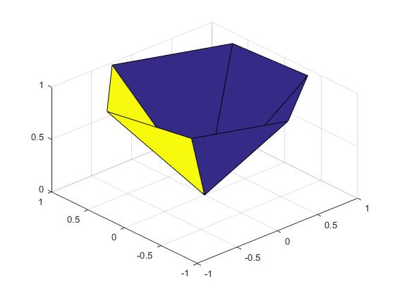
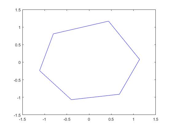
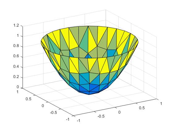
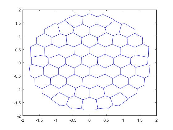
Fig. 2.1: A convex nodal function $u_{h}$ induces a convex piecewise linear function $\gamma_{h}=\Gamma(u_{h})$. The sub-differential $\partial u_{h}(0)$ of the convex nodal function $u_{h}$ at node $0$ is the convex hull of the piecewise gradients $\nabla\gamma_{h}|_{T}$, which is the polygon in the second figure. Let the domain $\Omega$ be a unit ball centered at $0$ and ${\mathcal{N}_{h}}$ be a nodal set in $\Omega$. A convex nodal function $u_{h}$ defined on ${\mathcal{N}_{h}}$ induces a piecewise linear function $\Gamma(u_{h})$. For each node $x_{i}\in{\mathcal{N}_{h}}$, there is an associated subdifferential $\partial u_{h}(x_{i})$ which corresponds to a polygon cell in the last figure. The piecewise gradient of $u_{h}$ can be viewed as a map between the domain $\Omega$ and the diagram.

To motivate the method introduced in [17], we first introduce the notion of an Alexandroff solution to the Monge-Ampère equation (1.1). To this end, note that if the solution to (1.1) is strictly convex, and if $u\in C^{2}(\Omega)$, then a change of variables reveals that

$$\int_{E}f\,dx=\int_{E}\det(D^{2}u)\,dx=\int_{\nabla u(E)}dx=|\nabla u(E)|\quad\text{for all Borel }E\subset\Omega,$$

where $|\nabla u(E)|$ denote the $d$-dimensional Lebesgue measure of $\nabla u(E)=\{\nabla u(x):\ x\in E\}$. To extend this identity to a larger class of functions, we introduce the subdifferential of the function $u$ at the point $x_{0}$ as

$$\partial u(x_{0})=\{p\in\mathbb{R}^{d}:\ u(x)\geq u(x_{0})+p\cdot(x-x_{0})\quad\forall x\in\Omega\}.$$

Thus, $\partial u(x_{0})$ is the set of supporting hyperplanes of the graph of $u$ at $x_{0}$. If $u$ is strictly convex and smooth then $\partial u(x_{0})=\{\nabla u(x_{0})\}$, and the same calculation as above shows that

$$\int_{E}f\,dx=|\partial u(E)|\quad\text{for all Borel }E\subset\Omega.$$ (2.4)

Definition 1.

A convex function $u\in C(\bar{\Omega})$ is an Alexandroff solution to (1.1) provided that $u=0$ on $\partial\Omega$ and (2.4) is satisfied.

The method introduced in [17] simply poses this solution concept onto the space of nodal functions. To do so, the definition of the subdifferential is extended to the spaces of nodal functions in the natural way:

$$\partial u_{h}(x_{i})=\{p\in\mathbb{R}^{d}:\ u(x_{j})\geq u_{h}(x_{i})+p\cdot(x_{j}-x_{j})\ \forall x_{j}\in{\mathcal{N}_{h}}\}.$$ (2.5)

To characterize the sub-differential of a nodal function $u_{h}$, we note that the convex envelope of a convex nodal function $u_{h}$, which is a piecewise linear function defined in $\Omega$, induces a mesh $\tilde{\mathcal{T}}_{h}$; see Figure 2.1. Then the sub-differential of $u_{h}$ at node $x_{i}$ can be characterized as the convex hull of the constant gradients $\bm{\nabla}\Gamma(u_{h})|_{T}$ for all $T\in\tilde{\mathcal{T}}_{h}$ which contain $x_{i}$; see Figure 2.1.

The discrete method is to find a convex nodal function $u_{h}$ with $u_{h}=0$ on ${\mathcal{N}_{h}^{B}}$ and

$$|\partial u_{h}(x_{i})|=f_{i}\qquad\forall x_{i}\in{\mathcal{N}_{h}^{I}},$$ (2.6)

where

$$f_{i}=\int_{\Omega}f(x)\phi_{i}(x)\,dx=\int_{\omega_{i}}f(x)\phi_{i}(x)\,dx.$$ (2.7)

Remark 2.1.

Existence and uniqueness of a solution to (2.6) is given in [17, 19].

2.3 Brunn Minkowski inequality and subdifferential of convex functions

In this subsection, we develop a few techniques which will be useful in establishing the error estimate. We start with the celebrated Brunn Minkowski inequality which relates the volumes of compact sets of $\mathbb{R}^{d}$.

Proposition 2.1 (Brunn Minkowski inequality).

Let $A$ and $B$ be two nonempty compact subsets of $\mathbb{R}^{d}$ for $d\geq 1$. Then the following inequality holds:

$$|A+B|^{1/d}\geq|A|^{1/d}+|B|^{1/d},$$

where $A+B$ denotes the Minkowski sum:

$$A+B:=\{v+w\in\mathbb{R}^{d}:v\in A\text{ and }w\in B\}.$$

Next, we make the following observation on the sum of two subdifferential sets.

Lemma 2 (Lemma 2.3 in [19]).

Let $u_{h}$ and $v_{h}$ be two convex nodal functions. Then there holds

$$\partial u_{h}(x_{i})+\partial v_{h}(x_{i})\subset\partial(u_{h}+v_{h})(x_{i})$$

for all $x_{i}\in{\mathcal{N}_{h}^{I}}$.

Proof.

Let $p_{1}$ and $p_{2}$ be in $\partial u_{h}(x_{i})$ and $\partial v_{h}(x_{i})$, respectively. By the definition of subdifferential (2.5), we have

$$p_{1}\cdot(x_{j}-x_{i})\leq u_{h}(x_{j})-u_{h}(x_{i})\quad\forall x_{j}\in{\mathcal{N}_{h}},$$

$$p_{2}\cdot(x_{j}-x_{i})\leq v_{h}(x_{j})-v_{h}(x_{i})\quad\forall x_{j}\in{\mathcal{N}_{h}}.$$

Adding both inequalites, we obtain

$$(p_{1}+p_{2})\cdot(x_{j}-x_{i})\leq(u_{h}+v_{h})(x_{j})-(u_{h}+v_{h})(x_{i})\quad\forall x_{j}\in{\mathcal{N}_{h}}.$$

This shows that $p_{1}+p_{2}\in\partial(u_{h}+v_{h})(x_{i})$. ∎

Combining both estimates, we derive the following result.

Lemma 3.

Let $u_{h}$ and $v_{h}$ be two convex nodal functions defined on ${\mathcal{N}_{h}}$ and $\mathcal{C}_{h}$ be the lower contact set of $(u_{h}-v_{h})$:

$$\mathcal{C}_{h}:=\big{\{}x_{i}\in{\mathcal{N}_{h}^{I}}:\ \Gamma(u_{h}-v_{h})(x_{i})=(u_{h}-v_{h})(x_{i})\big{\}}.$$

Then for any node $x_{i}\in\mathcal{C}_{h}$,

$$|\partial\Gamma(u_{h}-v_{h})(x_{i})|^{1/d}\leq|\partial u_{h}(x_{i})|^{1/d}-|\partial v_{h}(x_{i})|^{1/d}.$$ (2.8)

Proof.

The proof of this result is implicitly given in [19, Proposition 4.3], but we give it here for completeness.

The definition of the convex envelope and the subdifferential shows that

$$\partial\Gamma(u_{h}-v_{h})(x_{i})\subset\partial(u_{h}-v_{h})(x_{i})$$

for all $x_{i}\in\mathcal{C}_{\epsilon}$. Applying Lemma 2 then yields

$$\partial v_{h}(x_{i})+\partial\Gamma(u_{h}-v_{h})(x_{i})\subset\partial v_{h}(x_{i})+\partial(u_{h}-v_{h})(x_{i})\subset\partial u_{h}(x_{i}).$$

An application of the Brunn-Minkowski inequality (cf. Lemma 2.1) gets

$$|\partial v_{h}(x_{i})|^{1/d}+|\partial\Gamma(u_{h}-v_{h})(x_{i})|^{1/d} \leq|\partial v_{h}(x_{i})+\partial\Gamma(u_{h}-v_{h})(x_{i})|^{1/d}$$

$$\leq|\partial u_{h}(x_{i})|^{1/d}.$$

Rearranging terms we obtain (2.8). ∎

We also note that the numerical method (2.6) has a discrete comparison principle. Here, we refer to [19] for a proof.

Lemma 4 (discrete comparison principle, Corollary 4.4 in [19]).

Let $v_{h},w_{h}\in\mathcal{M}_{h}$ satisfy $v_{h}(x_{i})\geq w_{h}(x_{i})$ for all $x_{i}\in{\mathcal{N}_{h}^{B}}$ and $|\partial v_{h}(x_{i})|\leq|\partial w_{h}(x_{i})|$ for all $x_{i}\in{\mathcal{N}_{h}^{I}}$. Then

$$v_{h}(x_{i})\geq w_{h}(x_{i})\qquad\forall x_{i}\in{\mathcal{N}_{h}}.$$

3 Consistency of the Oliker-Prussner method

In this section, we state the consistency of the method (2.6) given in [19, Lemma 5.3, Proposition 5.4]. The result shows that the relative consistency error is of order $\mathcal{O}(h^{2})$ away from the boundary and of order $\mathcal{O}(1)$ in a $\mathcal{O}(h)$ region of the boundary.

Lemma 5.

Let ${\mathcal{N}_{h}}$ be translation invariant nodal set defined on the domain $\Omega$. If $u\in C^{k,\alpha}(\bar{\Omega})$ is a convex function with $0<\lambda I\leq D^{2}u\leq\Lambda I$ and $2\leq k+\alpha\leq 4$, there holds, for ${\rm dist}(x_{i},\partial\Omega)\geq Rh$,

$$\big{|}|\partial N_{h}u(x_{i})|-f_{i}\big{|}\leq Ch^{k+\alpha+d-2},$$ (3.1)

where $R$ depends on $\lambda$ and $\Lambda$. Moreover, there holds for ${\rm dist}(x_{i},\partial\Omega)\leq Rh$,

$$\big{|}\partial N_{h}u(x_{i})-f_{i}\big{|}\leq Ch^{d}.$$

Remark 3.1.

The regularity of $f$ and $\partial\Omega$, the strict convexity of $\Omega$, and the positivity of $f$ guarantees that the convex solution to (1.1) enjoys the regularity $u\in C^{k,\alpha}(\bar{\Omega})$. For example, if $f\in C^{k-2,\alpha}(\bar{\Omega})$ and $\Omega$ is smooth, then the solutions satisfies $u\in C^{k,\alpha}(\bar{\Omega})$ [11, 7, 20]

Thanks to the consistency error of the method, Lemma 5, an $L_{\infty}$-error estimate is derived in [19] which states

Proposition 6.

Let $\Omega$ be uniformly convex and ${\mathcal{N}_{h}^{I}}$ be translation invariant. Suppose further that the boundary nodes satisfy (2.1), that $f\geq\underline{f}>0$, and that the convex solution to (1.1) satisfies $u\in C^{k,\alpha}(\bar{\Omega})$ for some $2\leq k+\alpha\leq 4$ and $0<\lambda I\leq D^{2}u\leq\Lambda I$. Then the numerical solution to the discrete Monge-Ampère equation (2.6) satisfies

$$\|u_{h}-N_{h}u\|_{L_{\infty}({\mathcal{N}_{h}})}\leq Ch^{k+\alpha-2}\|u\|_{C^{k,\alpha}(\bar{\Omega})},$$

where $\|v_{h}\|_{L_{\infty}({\mathcal{N}_{h}})}:=\max_{x_{i}\in{\mathcal{N}_{h}}}|v_{h}(x_{i})|.$

We note that if $u\in C^{3,1}(\Omega)$, then the optimal order of the $L_{\infty}$ error is $\mathcal{O}(h^{2})$. By this $L_{\infty}$ error estimate and the assumption (2.1) that the boundary node is at least $h/2$ away from the boundary, we immediately deduce that $|\delta_{e}(N_{h}u-u_{h})(x_{i})|$ is bounded. This observation will be useful in the following sections when we investigate the discrete $W^{2}_{p}$ error estimate.

4 Stability of the Oliker-Prussner method

To derive the discrete $W^{2}_{p}$-estimate, we first make an observation that the contact set of a nodal function contains interesting information on its second order difference.

Lemma 7 (estimate of second order difference).

Given two convex nodal functions $v_{h}$ and $u_{h}$ defined on the nodal set ${\mathcal{N}_{h}}$, let

$$w_{\epsilon}=u_{h}-(1-\epsilon)v_{h}\quad\mbox{and}\quad w^{\epsilon}=v_{h}-(1-\epsilon)u_{h}$$

for some $0<\epsilon\leq 1$ and the contact sets

$$\mathcal{C}_{\epsilon}:= \;\{x_{i}\in{\mathcal{N}_{h}},\quad w_{\epsilon}(x_{i})=\Gamma w_{\epsilon}(x_{i})\},$$ (4.1)

$$\mathcal{C}^{\epsilon}:= \;\{x_{i}\in{\mathcal{N}_{h}},\quad w^{\epsilon}(x_{i})=\Gamma w^{\epsilon}(x_{i})\}.$$ (4.2)

If a node $x_{i}\in\mathcal{C}_{\epsilon}\cap\mathcal{C}^{\epsilon}$, then

$$-\epsilon\delta_{e}v_{h}(x_{i})\leq\delta_{e}(u_{h}-v_{h})(x_{i})\leq\frac{\epsilon}{1-\epsilon}\delta_{e}v_{h}(x_{i})$$ (4.3)

for any vector $e\in\mathbb{Z}^{d}$.

Proof.

We observe that if a node is in the contact set $x_{i}\in\mathcal{C}_{\epsilon}$, then the second order difference of $w_{\epsilon}$ satisfies $\delta_{e}w_{\epsilon}(x_{i})\geq\delta_{e}\Gamma w_{\epsilon}(x_{i})\geq 0$ for any vector $e\in\mathbb{Z}^{d}$. Hence, for any node $x_{i}\in\mathcal{C}_{\epsilon}$, we have

$$\delta_{e}(u_{h}-v_{h})(x_{i})\geq-\epsilon\delta_{e}v_{h}(x_{i}).$$ (4.4)

This inequality yields a lower bound of the second order difference.

To derive the upper bound, we apply a similar argument above to the function $w^{\epsilon}$ and derive

$$\delta_{e}(v_{h}-u_{h})(x_{i})\geq-\epsilon\delta_{e}u_{h}(x_{i})$$

for any node $x_{i}\in\mathcal{C}^{\epsilon}$. A simple algebraic manipulation yields

$$\delta_{e}(u_{h}-v_{h})(x_{i})\leq\frac{\epsilon}{1-\epsilon}\delta_{e}v_{h}(x_{i}).$$ (4.5)

Combining both the lower bound (4.4) and upper bound (4.5), we obtain the desired estimate. ∎

Remark 4.1.

The lemma above shows that we have control of the error $\delta_{e}(u_{h}-v_{h})$ on the contact sets $\mathcal{C}_{\epsilon}$ and $\mathcal{C}^{\epsilon}$. Define the set $E_{\tau}$ to be

$$E_{\tau}=\left\{x_{i}\in{\mathcal{N}_{h}},\ \delta_{e}(v_{h}-u_{h})(x_{i})\geq\tau\delta_{e}v_{h}(x_{i})\quad\mbox{for some vector $e\in\mathbb{Z}^{d}$}\right\},$$ (4.6)

where $\tau=\epsilon/(1-\epsilon)$. Then the proof of Lemma 7 shows that $E_{\tau}$ is contained in the non-contact set

$$S_{\epsilon}:={\mathcal{N}_{h}}\setminus\mathcal{C}_{\epsilon}.$$ (4.7)

Analogously,

$$E^{\tau}: =\left\{x_{i}\in{\mathcal{N}_{h}},\ \delta_{e}(u_{h}-v_{h})(x_{i})\geq\tau\delta_{e}v_{h}(x_{i})\quad\mbox{for some vector $e\in\mathbb{Z}^{d}$}\right\}$$

$$\subset S^{\epsilon}:={\mathcal{N}_{h}}\setminus\mathcal{C}^{\epsilon}.$$

In the next step, we estimate the cardinality of $S_{\epsilon}$. Heuristically, if $\epsilon=1$, then $w_{\epsilon}=u_{h}$ which is a convex nodal function, and so we have $S_{\epsilon}=\emptyset$. As $\epsilon$ decreases to zero, the function $w_{\epsilon}$ becomes ‘less convex’, and the cardinality $\#(S_{\epsilon})$ increases; see Figure 4.1. Therefore, our next goal is to estimate how fast $\#(S_{\epsilon})$ increases as $\epsilon\to 0$. The following lemma shows that this is controlled by the consistency error of the method.

Fig. 4.1: A pictorial description of Remark 4.1

Proposition 4.1.

Let $u_{h}$ and $v_{h}$ be two convex nodal functions satisfying $u_{h}=v_{h}$ on ${\mathcal{N}_{h}^{B}}$, $u_{h}\leq v_{h}$ in ${\mathcal{N}_{h}^{I}}$, and

$$|\partial u_{h}(x_{i})|=f_{i},\quad\mbox{ and }\quad|\partial v_{h}(x_{i})|=g_{i}$$ (4.8)

for all $x_{i}\in{\mathcal{N}_{h}^{I}}$. For any subset $S\subset{\mathcal{N}_{h}^{I}}$, let

$$\mu(S)=\sum_{x_{i}\in S}f_{i}\quad\mbox{and}\quad\nu_{\tau}(S)=\sum_{x_{i}\in S}\left(f_{i}^{1/d}+\frac{1}{\tau}e_{i}^{1/d}\right)^{d},$$ (4.9)

where $e_{i}^{1/d}=g_{i}^{1/d}-f_{i}^{1/d}$. Then

$$\mu(S_{\epsilon})\leq\nu_{\tau}(\mathcal{C}_{\epsilon})-\mu(\mathcal{C}_{\epsilon}),$$ (4.10)

where $\mathcal{C}_{\epsilon}$ is given by (4.1), $S_{\epsilon}$ is given by (4.7), and $\tau=\epsilon/(1-\epsilon)$. Consequently, there holds

$$\mu(S_{\epsilon})\leq\tau^{-1}C_{f}\|e^{1/d}\|_{\ell^{d}(\mathcal{C}_{\epsilon})},$$ (4.11)

with $C_{f}=d\|f^{1/d}\|_{\ell^{d}({\mathcal{N}_{h}^{I}})}^{d-1}.$

Proof.

We first show that

$$\sum_{x_{i}\in{\mathcal{N}_{h}^{I}}}\epsilon\partial u_{h}(x_{i})\subset\sum_{x_{i}\in{\mathcal{N}_{h}^{I}}}\partial\Gamma w_{\epsilon}(x_{i}),$$ (4.12)

where $w_{\epsilon}=u_{h}-(1-\epsilon)v_{h}$. Since $u_{h}\leq v_{h}$ in ${\mathcal{N}_{h}^{I}}$ and $u_{h}=v_{h}$ on ${\mathcal{N}_{h}^{B}}$, we get

$$w_{\epsilon}\leq\epsilon u_{h}\mbox{ in ${\mathcal{N}_{h}^{I}}$, }\quad\text{and}\quad w_{\epsilon}=\epsilon u_{h}\mbox{ on ${\mathcal{N}_{h}^{B}}$.}$$

Taking convex envelope on both side of the inequality, we obtain

$$\Gamma w_{\epsilon}(x)\leq\epsilon\Gamma u_{h}(x)\quad\mbox{in $\Omega$ and}\quad\Gamma w_{\epsilon}(x)=\epsilon\Gamma u_{h}(x)\quad\mbox{on $\partial\Omega$.}$$ (4.13)

Since $u_{h}=\Gamma u_{h}$ on ${\mathcal{N}_{h}}$ due to the convexity of $u_{h}$, the inequality (4.13) implies (4.12).

Taking measure on both sides of (4.12) and substituting (4.8) yields

$$\epsilon^{d}\sum_{x_{i}\in{\mathcal{N}_{h}^{I}}}f_{i}=\epsilon^{d}\sum_{x_{i}\in{\mathcal{N}_{h}^{I}}}|\partial u_{h}(x_{i})|\leq\sum_{x_{i}\in\mathcal{C}_{\epsilon}}|\partial\Gamma w_{\epsilon}(x_{i})|.$$

In view of the convexity of the measure of the subidfferential (2.8),

$$|\partial\Gamma w_{\epsilon}(x_{i})|^{1/d}\leq|f^{1/d}_{i}-(1-\epsilon)g^{1/d}_{i}|.$$

Therefore, we infer that

$$\epsilon^{d}\mu({\mathcal{N}_{h}^{I}})=\epsilon^{d}\sum_{x_{i}\in{\mathcal{N}_{h}^{I}}}f_{i}\leq\sum_{x_{i}\in\mathcal{C}_{\epsilon}}|f^{1/d}_{i}-(1-\epsilon)g^{1/d}_{i}|^{d}.$$

Thus, subtracting $\epsilon^{d}\mu(\mathcal{C}_{\epsilon})$, we obtain

$$\epsilon^{d}\mu(S_{\epsilon})=\epsilon^{d}\sum_{x_{i}\in S_{\epsilon}}f_{i}\leq \;\sum_{x_{i}\in\mathcal{C}_{\epsilon}}\big{(}|\epsilon f^{1/d}_{i}+(1-\epsilon)e_{i}^{1/d}|^{d}-\epsilon^{d}f_{i}\big{)}.$$

Therefore, dividing $\epsilon^{d}$, we obtain

$$\mu(S_{\epsilon})\leq\nu_{\tau}(\mathcal{C}_{\epsilon})-\mu(\mathcal{C}_{\epsilon}).$$

To derive the estimate (4.11), we first see that (4.10) is equivalent to

$$\|f^{1/d}\|_{\ell^{d}({\mathcal{N}_{h}^{I}})}\leq\|f^{1/d}+\tau^{-1}e^{1/d}\|_{\ell^{d}(\mathcal{C}_{\epsilon})},$$

and therefore $\|f^{1/d}\|_{\ell^{d}({\mathcal{N}_{h}^{I}})}-\|f^{1/d}\|_{\ell^{d}(\mathcal{C}_{\epsilon})}\leq\tau^{-1}\|e^{1/d}\|_{\ell^{d}(\mathcal{C}_{\epsilon})}$ by the Minkowski inequality. From this estimate and the inequality $a^{d}-b^{d}\leq da^{d-1}(a-b)$ for $a\geq b$, we derive

$$\mu(S_{\epsilon}) =\|f^{1/d}\|_{\ell^{d}({\mathcal{N}_{h}^{I}})}^{d}-\|f^{1/d}\|_{\ell^{d}(\mathcal{C}_{\epsilon})}^{d}$$

$$\leq d\|f^{1/d}\|_{\ell^{d}({\mathcal{N}_{h}^{I}})}^{d-1}\big{(}\|f^{1/d}\|_{\ell^{d}({\mathcal{N}_{h}^{I}})}-\|f^{1/d}\|_{\ell^{d}(\mathcal{C}_{\epsilon})}\big{)}$$

$$\leq C_{f}\tau^{-1}\|e^{1/d}\|_{\ell^{d}(\mathcal{C}_{\epsilon})}.$$

∎

5 $W^{2}_{p}$-estimate of the method

To establish $W^{2}_{p}$-estimates of the method, we first introduce an estimate of the discrete $L_{1}$ norm of a nodal function in terms of its level sets.

Lemma 8.

Let $s_{h}$ be a bounded nodal function with $|s_{h}(x_{i})|\leq M$ for some $M>0$. Then, for any $\sigma>0$,

$$\sum_{x_{i}\in{\mathcal{N}_{h}^{I}}}f_{i}|s_{h}(x_{i})|\leq\sigma\sum_{k=0}^{N}\mu(A_{k}),$$

where

$$A_{k}:=\{x_{i}\in{\mathcal{N}_{h}^{I}}:\ |s_{h}(x_{i})|\geq k\sigma\},$$

$\mu(\cdot)$ is given by (4.9), and $N=\lceil M/\sigma\rceil$.

Proof.

The estimate is illustrated in the Figure 5.1. Here, we give a rigorous proof.
Set

$$P_{k}:=\{x_{i}\in{\mathcal{N}_{h}^{I}}:\ k\sigma\leq|s_{h}(x_{i})|<(k+1)\sigma\}.$$

Then we clearly have

$$\sum_{x_{i}\in{\mathcal{N}_{h}^{I}}}f_{i}|s_{h}(x_{i})|=\sum_{k=0}^{N}\sum_{x_{i}\in P_{k}}f_{i}|s_{h}(x_{i})|\leq\sum_{k=0}^{N}(k+1)\sigma\mu(P_{k}).$$

We also have

$$A_{k}=\bigcup_{m\geq k}^{N}P_{m},$$

and so, since the sets $\{P_{k}\}$ are disjoint,

$$\mu(A_{k})=\sum_{m=k}^{N}\mu(P_{m}).$$

Therefore

$$\sigma\sum_{k=0}^{N}\mu(A_{k})=\sigma\sum_{k=0}^{N}\sum_{m=k}^{N}\mu(P_{m})=\sigma\sum_{k=0}^{N}(k+1)\mu(P_{k})\geq\sum_{x_{i}\in{\mathcal{N}_{h}^{I}}}f_{i}|s_{h}(x_{i})|.$$

∎

Fig. 5.1: A pictorial illustration of Lemma 8. Here, the measure $\mu(A_{k}):=\sum_{x_{i}\in A_{k}}f_{i}$.

5.1 Ideal Case

Now we are ready to prove the estimate in the case that the consistency error (3.1) holds for all interior grid points.

Theorem 9.

Let $u$ be the solution of the Monge-Ampère equation (1.1). Assume that

$$\big{|}|\partial N_{h}u(x_{i})|-f_{i}\big{|}\leq Ch^{2+d}\quad\mbox{ for every node $x_{i}\in{\mathcal{N}_{h}^{I}}$,}$$ (5.1)

where $N_{h}u$ is the interpolation of $u$ on the nodal set ${\mathcal{N}_{h}}$. Assume further that $f$ is uniformly positive on $\Omega$. Then the error in the weighted $W^{2}_{p}$-norm satisfies

$$\|N_{h}u-u_{h}\|_{W^{2}_{p}({\mathcal{N}_{h}^{I}})}\leq C\left\{\begin{array}[]{ll}h^{2}|\ln h|&\text{if $p=1$},\\ h^{2/p}&\text{if $p>1$}\end{array}\right.$$

provided that $h$ is sufficiently small.

Proof.

We start by setting $v_{h}=(1-Ch^{2})^{1/d}N_{h}u$, where the constant $C>0$ is large enough, but independent of $h$, to ensure that (cf. (5.1))

$$g_{i}:=|\partial v_{h}(x_{i})|=(1-Ch^{2})|\partial N_{h}u(x_{i})|\leq f_{i}.$$

By a comparison principle (cf. Lemma 4), we have $u_{h}\leq v_{h}$ on ${\mathcal{N}_{h}^{I}}$, and we see that

$$|f_{i}-g_{i}|\leq Ch^{2+d}\qquad\forall x_{i}\in{\mathcal{N}_{h}^{I}}$$ (5.2)

due to the assumption (5.1). We also have $g_{i}\geq Ch^{d}$ provided $h$ is sufficiently small, and $|(v_{h}-N_{h}u)(x_{i})|\leq Ch^{2}$.

Note that

$$\|N_{h}u-u_{h}\|_{W^{2}_{p}({\mathcal{N}_{h}^{I}})}\leq\|v_{h}-u_{h}\|_{W^{2}_{p}({\mathcal{N}_{h}^{I}})}+Ch^{2}\|N_{h}u\|_{W^{2}_{p}({\mathcal{N}_{h}^{I}})}$$

Thus, to prove the theorem, it suffices to show that

$$\sum_{x_{i}\in{\mathcal{N}_{h}^{I}}}f_{i}|\delta_{e}(v_{h}-u_{h})(x_{i})|^{p}\leq C\left\{\begin{array}[]{ll}h^{2}|\ln h|&\text{if $p=1$},\\ h^{2}&\text{if $p>1$}.\end{array}\right.$$

Define the positive and negative parts of $\delta_{e}(v_{h}-u_{h})(x_{i})$, respectively, as

$$\delta_{e}^{+}(v_{h}-u_{h})(x_{i}) =\max\{\delta_{e}(v_{h}-u_{h})(x_{i}),0\},$$

$$\delta_{e}^{-}(v_{h}-u_{h})(x_{i}) =\max\{-\delta_{e}(v_{h}-u_{h})(x_{i}),0\}.$$

We shall prove

$$\sum_{x_{i}\in{\mathcal{N}_{h}^{I}}}f_{i}|\delta_{e}^{+}(v_{h}-u_{h})(x_{i})|^{p}\leq C\left\{\begin{array}[]{ll}h^{2}|\ln h|&\text{if $p=1$},\\ h^{2}&\text{if $p>1$}.\end{array}\right.$$

The estimate for the negative part can be proved in a similar fashion.

Due to the regularity assumption of $u$, a Taylor expansion shows that $|\delta_{e}v_{h}(x_{i})|\leq C_{2}$ for all $x_{i}\in{\mathcal{N}_{h}^{I}}$, where $C_{2}>0$ depends on $\|u\|_{C^{1,1}(\bar{\Omega})}$. Moreover, from the $L_{\infty}$ error estimate, Proposition 6 and the assumption (2.1) that interior nodes are at least $h/2$ away from the boundary, we deduce that

$$\delta_{e}^{+}(v_{h}-u_{h})(x_{i})\leq C_{\infty}\qquad\forall x_{i}\in{\mathcal{N}_{h}^{I}},$$

where the constant $C_{\infty}>0$ depends on $\|u\|_{C^{3,1}(\bar{\Omega})}$.

Let $\tau_{k}=C_{2}k^{1/p}h^{2}$, and define the set

$$A_{k}:=\{x_{i}\in{\mathcal{N}_{h}^{I}},\quad\delta^{+}_{e}(v_{h}-u_{h})(x_{i})\geq\tau_{k}\}.$$

By Lemma 8 with $s_{h}(x_{i})=|\delta_{e}^{+}(v_{h}-u_{h})(x_{i})|^{p}$, $\sigma=C^{p}_{2}h^{2p}$, and $M=C_{\infty}^{p}$, we obtain

$$\sum_{x_{i}\in{\mathcal{N}_{h}^{I}}}f_{i}|\delta_{e}^{+}(v_{h}-u_{h})(x_{i})|^{p}\leq \;Ch^{2p}\left(\mu({\mathcal{N}_{h}^{I}})+\sum_{k=1}^{Ch^{-2p}}\mu(A_{k})\right).$$ (5.3)

We aim to estimate the measure of set $\mu(A_{k})$. Due to the relations of the second order difference and contact set given in Remark 4.1, we have $A_{k}\subset S_{\epsilon_{k}}={\mathcal{N}_{h}^{I}}\setminus\mathcal{C}_{\epsilon_{k}}$ with $\epsilon_{k}\in(0,1)$ satisfying $\tau_{k}=\epsilon_{k}/(1-\epsilon_{k})$. Therefore, by the estimate (4.11) given in Proposition 4.1,

$$\mu(A_{k})\leq\mu(S_{\epsilon_{k}})\leq\frac{C_{f}}{\tau_{k}}\|g^{1/d}-f^{1/d}\|_{\ell^{d}(\mathcal{C}_{\epsilon_{k}})}=\frac{C_{f}}{k^{1/p}h^{2}}\|g^{1/d}-f^{1/d}\|_{\ell^{d}(\mathcal{C}_{\epsilon_{k}})}.$$

From the concavity of $t\to t^{1/d}$, we have $(t+\epsilon)^{1/d}-t^{1/d}\leq d^{-1}t^{1/d-1}\epsilon$. Setting $t=g_{i}$ and $\epsilon=f_{i}-g_{i}\geq 0$, we get

$$|f_{i}^{1/d}-g_{i}^{1/d}|=f_{i}^{1/d}-g_{i}^{1/d}\leq d^{-1}g_{i}^{1/d-1}(f_{i}-g_{i})\leq Ch^{3}$$

due to the consistency error (5.2) and the lower bound $g_{i}\geq Ch^{d}$. Consequently, we find that

$$\|\,f^{1/d}-g^{1/d}\,\|_{\ell^{d}(\mathcal{C}_{\epsilon_{k}})}\leq Ch^{2},$$

and therefore $\mu(A_{k})\leq\frac{C}{k^{1/p}}$. Applying this bound in (5.3), we derive the estimate

$$\sum_{x_{i}\in{\mathcal{N}_{h}^{I}}}f_{i}|\delta_{e}^{+}(u_{h}-v_{h})(x_{i})|^{p}\leq \;Ch^{2p}\sum_{k=1}^{Ch^{-2p}}\frac{1}{k^{1/p}}\leq C\left\{\begin{array}[]{ll}h^{2}|\ln h|&\text{if $p=1$},\\ h^{2}&\text{if $p>1$}.\end{array}\right.$$

This completes the proof. ∎

Remark 5.1.

It is worth mentioning that the assumption on the consistency error (5.1) holds for nodes bounded away from the boundary $\partial\Omega$ provided that $u\in C^{3,1}(\Omega)$. However, for nodes close to the boundary $\partial\Omega$, such an estimate holds only for structured domain, such as a rectangle domain; see the first numerical experiment in Section 6. In general, this estimate may not be true. In fact, Lemma 5 shows that the (relative) consistency error, $\mathcal{O}(h)$ away from the boundary, is of order $\mathcal{O}(1)$. In the following subsection, we take into account the lack of consistency in the boundary layer.

5.2 Estimate on general domain

To this end, we define the barrier nodal function

$$b_{h}(x_{i})=\begin{cases}-h^{2}\quad&\text{if }x_{i}\in{\mathcal{N}_{h}^{I}},\\ 0\quad&\text{if }x_{i}\in{\mathcal{N}_{h}^{B}},\end{cases}$$

which will be used to “push down” the graph of the nodal interpolant of $u$ and as such, develop error estimates in a general setting.

Theorem 10.

Let $u\in C^{3,1}(\bar{\Omega})$ be the solution of the Monge-Ampère equation (1.1) with $0<\lambda I\leq D^{2}u\leq\Lambda I$, and assume that the nodal set ${\mathcal{N}_{h}^{I}}$ translation invariant and that $f$ is uniformly positive on $\Omega$. Then the error in the weighted $W^{2,p}$-norm satisfies

$$\|N_{h}u-u_{h}\|_{W^{2}_{p}({\mathcal{N}_{h}^{I}})}\leq C\begin{cases}h^{1/p}\quad&\mbox{if $p>d$,}\\ h^{1/d}\big{(}\ln\left(\frac{1}{h}\right)\big{)}^{1/d}\quad&\mbox{if $p\leq d$,}\end{cases}$$

where $N_{h}u$ is the interpolation of $u$ on the nodal set ${\mathcal{N}_{h}}$ and the constant $C$ depends on $\|u\|_{C^{3,1}(\bar{\Omega})}$, the dimension $d$, and the constant $p$.

Proof.

We define the boundary layer:

$$\Omega_{h}:=\{x_{i}\in{\mathcal{N}_{h}^{I}},\textrm{dist}(x_{i},\partial\Omega)\leq Rh\},$$

where the constant $R$ is the constant in the consistency error, Lemma 5, which depends on the ellipticity constants $\lambda$ and $\Lambda$ of $D^{2}u$. We set

$$v_{h}=N_{h}u-Cb_{h},\qquad g_{i}=|\partial v_{h}(x_{i})|,$$

where the constant $C>0$ is sufficiently large so that $u_{h}\leq v_{h}$; see Proposition 6. It is clear from the definition of $b_{h}$ that

$$|\partial v_{h}(x_{i})|=|\partial N_{h}u(x_{i})|\quad\mbox{for any $x_{i}\in{\mathcal{N}_{h}^{I}}\setminus\Omega_{h}$}$$

and

$$|\partial N_{h}u(x_{i})|\geq|\partial v_{h}(x_{i})|\geq 0\quad\mbox{for any $x_{i}\in\Omega_{h}$}.$$

This implies that $|f_{i}-g_{i}|\leq Ch^{2+d}$ in ${\mathcal{N}_{h}^{I}}\setminus\Omega_{h}$ and $|f_{i}-g_{i}|\leq Ch^{d}$ in $\Omega_{h}$. We have that $|\delta_{e}v_{h}(x_{i})|\leq C_{2}$ and $|\delta_{e}(v_{h}-u_{h})(x_{i})|\leq C_{\infty}$ for all $x_{i}\in{\mathcal{N}_{h}^{I}}$. As in Theorem 9, we shall prove the estimate for the positive part:

$$\sum_{x_{i}\in{\mathcal{N}_{h}^{I}}}f_{i}\left(\delta_{e}^{+}(v_{h}-u_{h})(x_{i})\right)^{p}\leq\begin{cases}Ch\quad&\mbox{if $p>d$,}\\ Ch\ln\left(\frac{1}{h}\right)\quad&\mbox{if $p=d$.}\end{cases}$$

The estimate for the negative part can be proved in a similar fashion. Also note that the estimate for $p<d$ follows from the estimate of $p=d$ and Hölder’s inequality:

$$\|N_{h}u-u_{h}\|_{W^{2}_{p}({\mathcal{N}_{h}^{I}})}\leq C_{\mu}\|N_{h}u-u_{h}\|_{W^{2}_{d}({\mathcal{N}_{h}^{I}})}\quad\mbox{where }C_{\mu}:=\mu({\mathcal{N}_{h}^{I}})^{1/p-1/d}.$$

We set $\tau_{k}=C_{2}k^{1/p}h$ and define the set

$$A_{k}:=\{x_{i}\in{\mathcal{N}_{h}^{I}},\quad\left(\delta^{+}_{e}(v_{h}-u_{h})(x_{i})\right)\geq\tau_{k}\}.$$

Then, by similar arguments as in Theorem 9, we find by Lemma 8 that

$$\sum_{x_{i}\in{\mathcal{N}_{h}^{I}}}f_{i}\left(\delta_{e}^{+}(v_{h}-u_{h})(x_{i})\right)^{p}\leq \;C_{2}h^{p}\left(\mu({\mathcal{N}_{h}^{I}})+\sum_{k=1}^{h^{-p}}\mu(A_{k})\right).$$ (5.4)

To estimate the measure of set $\mu(A_{k})$, we note that $A_{k}\subset S_{\epsilon_{k}}={\mathcal{N}_{h}^{I}}\setminus\mathcal{C}_{\epsilon_{k}}$ with $\tau_{k}=\epsilon_{k}/(1-\epsilon_{k})$. Invoking the estimate of the measure of the non-contact set $S_{\epsilon}$ stated in Proposition 4.1, we obtain

$$\mu(A_{k})\leq\mu(S_{\epsilon_{k}})\leq\nu_{\tau_{k}}(\mathcal{C}_{\epsilon_{k}})-\mu(\mathcal{C}_{\epsilon_{k}}).$$

We then divide the estimate of $\nu_{\tau_{k}}(\mathcal{C}_{\epsilon_{k}})-\mu(\mathcal{C}_{\epsilon_{k}})$ into two parts:

$$\nu_{\tau_{k}}(\mathcal{C}_{\epsilon_{k}})-\mu(\mathcal{C}_{\epsilon_{k}})= \;\sum_{x_{i}\in\mathcal{C}_{\epsilon_{k}}}\left[\left(f_{i}^{1/d}+\frac{1}{\tau_{k}}e_{i}^{1/d}\right)^{d}-f_{i}\right]$$

$$= \;\left(\sum_{x_{i}\in\mathcal{C}_{\epsilon_{k}}\cap\Omega_{h}}+\sum_{x_{i}\in\mathcal{C}_{\epsilon_{k}}\setminus\Omega_{h}}\right)\left[\left(f_{i}^{1/d}+\frac{1}{\tau_{k}}e_{i}^{1/d}\right)^{d}-f_{i}\right],$$

where we recall that $e_{i}^{1/d}=f_{i}^{1/d}-g_{i}^{1/d}$. Since $f_{i}^{1/d}=\mathcal{O}(h)$ and $g_{i}^{1/d}=\mathcal{O}(h)$, we have

$$\left|\left(f_{i}^{1/d}+\frac{1}{\tau_{k}}e_{i}^{1/d}\right)^{d}-f_{i}\right| \leq\frac{d}{\tau_{k}}\max\{\big{|}f_{i}^{1/d}+\frac{1}{\tau_{k}}e_{i}^{1/d}\big{|},f_{i}^{1/d}\}^{d-1}|e_{i}^{1/d}|$$

$$\leq\frac{Ch^{d-1}}{\tau_{k}^{d}}|e_{i}^{1/d}|.$$

In the set $\mathcal{C}_{\epsilon_{k}}\cap\Omega_{h}$, the consistency error satisfies $|e_{i}^{1/d}|=\mathcal{O}(h)$; see Lemma 5. Therefore, we have

$$\left|\left(f_{i}^{1/d}+\frac{1}{\tau_{k}}e_{i}^{1/d}\right)^{d}-f_{i}\right|\leq\frac{Ch^{d}}{\tau_{k}^{d}}\qquad\forall x_{i}\in\mathcal{C}_{\epsilon_{k}}\cap\Omega_{h}.$$

On the other hand, in the set $\mathcal{C}_{\epsilon_{k}}\setminus\Omega_{h}$, we conclude as in Theorem 9, that $|e_{i}^{1/d}|=\mathcal{O}(h^{3})$, and

$$\left|\left(f_{i}^{1/d}+\frac{1}{\tau_{k}}e_{i}^{1/d}\right)^{d}-f_{i}\right|\leq\frac{Ch^{2+d}}{\tau_{k}^{d}}.$$

Combining both estimate and applying the fact that $\#(\mathcal{C}_{\epsilon_{k}}\cap\Omega_{h})\leq Ch^{1-d}$ and $\#(\mathcal{C}_{\epsilon_{k}}\setminus\Omega_{h})\leq Ch^{-d}$, we obtain

$$\nu_{\tau_{k}}(\mathcal{C}_{\epsilon})-\mu(\mathcal{C}_{\epsilon})\leq\frac{Ch}{\tau_{k}^{d}}+\frac{Ch^{2}}{\tau_{k}^{d}}\leq\frac{Ch}{\tau_{k}^{d}}$$

because $h\leq 1$. Hence, we conclude that

$$\mu(A_{k})\leq\frac{Ch}{\tau_{k}^{d}}.$$

Applying this estimate to (5.4), we arrive at

$$\sum_{x_{i}\in{\mathcal{N}_{h}^{I}}}f_{i}|\delta_{e}^{+}(v_{h}-u_{h})(x_{i})|^{p}\leq C_{2}h^{p}\sum_{k=1}^{h^{-p}}\frac{h}{h^{d}k^{d/p}}.$$

Since

$$\sum_{k=1}^{h^{-p}}\frac{1}{k^{d/p}}\leq\begin{cases}C(d,p)h^{d-p}\quad&\mbox{if $p>d$,}\\ C\ln\left(\frac{1}{h}\right)\quad&\mbox{if $p=d$,}\end{cases}$$

we conclude that

$$\sum_{x_{i}\in{\mathcal{N}_{h}^{I}}}f_{i}|\delta_{e}^{+}(v_{h}-u_{h})(x_{i})|^{p}\leq\begin{cases}Ch\quad&\mbox{if $p>d$,}\\ Ch\ln\left(\frac{1}{h}\right)\quad&\mbox{if $p=d$.}\end{cases}$$

Finally we note that by Hölder’s inequality, there holds for $p<d$,

$$\|v_{h}\|_{W^{2}_{p}({\mathcal{N}_{h}^{I}})} =\Big{(}\sum_{x_{i}\in{\mathcal{N}_{h}^{I}}}f_{i}|\delta_{e}v_{h}(x_{i})|^{p}\Big{)}^{1/p}$$

$$\leq\big{(}\sum_{x_{i}\in{\mathcal{N}_{h}^{I}}}f_{i}|\delta_{e}v_{h}(x_{i})|^{d}\Big{)}^{1/d}\Big{(}\sum_{x_{i}\in{\mathcal{N}_{h}^{I}}}f_{i}\Big{)}^{(d-p)/(dp)}\leq C\|v_{h}\|_{W^{2}_{d}({\mathcal{N}_{h}^{I}})}.$$

This completes the proof. ∎

6 Numerical experiments

In this section, we perform numerical examples to illustrate the accuracy of the method, and to compare the results with the theory. In the tests, we replace the homogeneous boundary condition (1.1b) with $u=g$ on $\partial\Omega$. The theoretical results developed in the previous sections can be applied to this slightly more general problem with minor modifications.

We consider three different test problems, each reflecting different scenarios of regularity. Each set of problems is performed in two dimensions ($d=2$), and errors are reported in the (discrete) $L_{\infty}$, $H^{1}$, $W_{1}^{2}$, and $W^{2}_{2}$ norms. Here, a nine-point stencil is used in the definition of the $W^{2}_{p}$ norms with $e_{1}=(1,0)$, $e_{2}=(0,1)$, $e_{3}=(1,1)$ and $e_{4}=(1,-1)$. That is, with an abuse of notation, we set

$$\|v\|_{W^{2}_{p}({\mathcal{N}_{h}^{I}})}^{p}=\sum_{j=1}^{4}\sum_{x_{i}\in{\mathcal{N}_{h}^{I}}}|\delta_{e_{j}}v(x_{i})|^{p}.$$

As explained in [19] and in Section 2.2, a convex nodal function induces a triangulation of $\Omega$ whose set of vertices corresponds to ${\mathcal{N}_{h}}$. For a computed solution $u_{h}$, we associate with it a piecewise linear polynomial on the induced mesh, which we still denote by $u_{h}$, and use the quantity $\|u-u_{h}\|_{H^{1}(\Omega)}$ to denote the $H^{1}$ error in the experiments below.

A summary of the theoretical results in Sections 2.3 and 5 when $d=2$ are

$$\|N_{h}u-u_{h}\|_{L_{\infty}({\mathcal{N}_{h}^{I}})}=\mathcal{O}(h^{2}),\qquad\|N_{h}u-u_{h}\|_{W^{2}_{p}({\mathcal{N}_{h}^{I}})}=\mathcal{O}(h^{1/2-\epsilon}),\ p=1,2$$

for any $\epsilon>0$, provided that $u\in C^{3,1}(\bar{\Omega})$.

Example I: Smooth Solution $u\in C^{\infty}(\bar{\Omega})$

We consider the example

$$u(x,y)=e^{\frac{x^{2}+y^{2}}{2}},\quad f(x,y)=(1+x^{2}+y^{2})e^{x^{2}+y^{2}},\quad\text{and }\Omega=(-1,1)^{2},$$ (6.1)

and list the resulting errors and rates of the scheme in Table 6.1. The Table clearly shows that the errors decay with rate $\mathcal{O}(h^{2})$ in all norms. This behavior matches the theoretical results of Proposition 6, but indicates that the $W^{2}_{p}$ estimates stated in Theorem 10 are not sharp.

$h$	$L_{\infty}$	rate	$H^{1}$	rate	$W^{2}_{1}$	rate	$W^{2}_{2}$	rate
1	1.12e-01	0.00	2.24e-01		4.49e-01		1.44e+01
1/2	4.78e-02	1.23	1.35e-01	0.73	6.02e-01	-0.42	4.24e-01	5.08
1/4	1.37e-02	1.80	4.35e-02	1.63	2.94e-01	1.03	1.93e-01	1.13
1/8	3.55e-03	1.95	1.16e-02	1.91	9.93e-02	1.57	6.34e-02	1.61
1/16	8.96e-04	1.99	2.94e-03	1.98	2.86e-02	1.80	1.80e-02	1.82
1/32	2.24e-04	2.00	7.39e-04	1.99	7.66e-03	1.90	4.79e-03	1.91
1/64	5.61e-05	2.00	1.85e-04	2.00	1.98e-03	1.95	1.24e-03	1.95

Table 6.1: Rate of convergence for a smooth solution (Example I).

Example II: Piecewise Smooth Solution $u\in W^{2}_{\infty}$

In this example, the domain is $\Omega=(-1,1)^{2}$, and the exact solution and data are taken to be

$$u(x)= \left\{\begin{array}[]{ll}2|x|^{2}&\text{in $|x|\leq 1/2$},\\ 2(|x|-1/2)^{2}+2|x|^{2}&\text{in $1/2\leq|x|$},\end{array}\right.$$

$$f(x)= \left\{\begin{array}[]{ll}16&\text{in $|x|\leq 1/2$},\\ 64-16|x|^{-1}&\text{in $1/2\leq|x|$}.\end{array}\right.$$

A simple calculation shows that $u\in C^{1,1}(\bar{\Omega})$ and $u\in C^{4}(\Omega\setminus\partial B_{1})$, but $u\not\in C^{2}(\bar{\Omega})$. The errors and rates of convergence are given in Table 6.2. The table shows that, while all errors tend to zero as the mesh is refined, the rates of convergence in the $L_{\infty}$ and $W^{2}_{1}$ norms are less obvious than the previous set of experiments. Nonetheless, while Theorem 10 assumes more regularity of the exact solution, we do observe a convergence rate of approximately $\mathcal{O}(h^{1/2})$ in the $W^{2}_{2}$ as stated in the theorem.

$h$	$L_{\infty}$	rate	$H^{1}$	rate	$W^{2}_{1}$	rate	$W^{2}_{2}$	rate
1	4.02e-01	0.00	8.04e-01	0.00	1.61	0.00	1.61	0.00
1/2	4.19e-02	3.26	1.30e-01	2.63	6.08e-01	1.40	5.39e-01	1.58
1/4	2.89e-02	0.53	6.84e-02	0.92	6.46e-01	-0.09	5.54e-01	-0.04
1/8	1.27e-02	1.18	3.50e-02	0.97	5.14e-01	0.33	4.54e-01	0.29
1/16	4.58e-03	1.47	1.38e-02	1.34	2.76e-01	0.90	3.15e-01	0.53
1/32	8.02e-04	2.51	3.59e-03	1.94	1.08e-01	1.35	2.08e-01	0.60
1/64	4.33e-04	0.89	1.50e-03	1.26	6.36e-02	0.77	1.56e-01	0.42

Table 6.2: Rate of convergence of piecewise smooth viscosity solution (Example II).

Example III: Singular Solution $u\in W^{2}_{p}$ with $p<2$

In the last series of experiments, the domain is $\Omega=(-1,1)^{2}$, and the solution and data are

$$u(x) =\left\{\begin{array}[]{ll}x^{4}+\frac{3}{2}y^{2}/x^{2}&\text{in $|y|\leq|x|^{3}$},\\ \frac{1}{2}x^{2}y^{2/3}+2y^{4/3}&\text{in $|y|\geq|x|^{3}$},\end{array}\right.$$

$$f(x)= \left\{\begin{array}[]{ll}36-9y^{2}/x^{6}&\text{in $|y|\leq|x|^{3}$},\\ \frac{8}{9}-\frac{5}{9}x^{2}/y^{2/3}&\text{in $|y|>|x|^{3}$}.\end{array}\right.$$

This example is constructed in [21] to show that $D^{2}u(x)$ may not be in $W^{2}_{p}$ for large $p$ for discontinuous $f$. The errors of the method for this problem are listed in Table 6.3. Because the exact solution does not enjoy $W^{2}_{2}$ regularity, it is not expected that the discrete solution will converge in the discrete $W^{2}_{2}$ norm, and this is observed in the table. However, we do observe convergence in the $L_{\infty}$, $H^{1}$, and $W^{2}_{1}$ norms with approximate rates $\|N_{h}u-u_{h}\|_{L_{\infty}({\mathcal{N}_{h}^{I}})}=\mathcal{O}(h^{4/3})$, $\|N_{h}u-u_{h}\|_{H^{1}({\mathcal{N}_{h}^{I}})}=\mathcal{O}(h)$, and $\|N_{h}u-u_{h}\|_{W^{2}_{1}({\mathcal{N}_{h}^{I}})}=\mathcal{O}(h^{1/2})$.

$h$	$L_{\infty}$	rate	$H^{1}$	rate	$W^{2}_{1}$	rate	$W^{2}_{2}$	rate
1	8.36e-01	0.00	1.67	0.00	3.35	0.00	3.35	0.00
1/2	2.34e-01	1.84	9.11e-01	0.88	5.48	-0.71	3.94	-0.24
1/4	1.86e-01	0.33	4.80e-01	0.92	4.90	0.16	4.02	-0.03
1/8	8.52e-02	1.13	2.41e-01	1.00	4.00	0.29	3.94	0.03
1/16	3.41e-02	1.32	1.02e-01	1.24	2.38	0.75	3.33	0.24
1/32	1.35e-02	1.34	4.79e-02	1.09	1.59	0.58	3.17	0.07

Table 6.3: Rate of convergence of $W^{2}_{p}$ solution with $p<2$ (Example III).

References

- [1] G. Awanou, Quadratic mixed finite element approximations of the Monge-Ampère equation in 2D, Calcolo 52, 503–518, 2015.
- [2] G. Awanou, Spline element method for Monge-Ampère equations , B.I.T., 55, 625–646, 2015.
- [3] G. Barles and P. E. Souganidis, Convergence of approximation schemes for fully nonlinear second order equations, Asymptotic Anal., 4:271–283, 1991.
- [4] K. Böhmer, On finite element methods for fully nonlinear elliptic equations of second order, SIAM J. Numer. Anal., 46(3):1212–1249, 2008.
- [5] J. D. Benamou, F. Collino, and J. M. Mirebeau, Monotone and consistent discretization of the Monge-Ampère operator, Math. Comp., 85(302):2743–2775, 2016.
- [6] S. C. Brenner, T. Gudi, M. Neilan, and L-Y. Sung, penalty methods for the fully nonlinear Monge-Ampère equation, Math. Comp., 80(276):1979–1995, 2011.
- [7] L. Caffarelli, L. Nirenberg, and J. Spruck, The Dirichlet problem for nonlinear second-order elliptic equations. I. Monge-Ampère equation, Comm. Pure Appl. Math., 37(3):369–402, 1984.
- [8] X. Feng and M. Neilan, Vanishing moment method and moment solutions for fully nonlinear second order partial differential equations, J. Sci. Comput., 38(1):74–98, 2009.
- [9] X. Feng and M. Jensen, Convergent semi-Lagrangian methods for the Monge-Ampère equation on unstructured grids, SIAM J. Numer. Anal., 55(2), 691–712, 2017.
- [10] B. D. Froese and A. M. Oberman, Convergent finite difference solvers for viscosity solutions of the elliptic Monge-Ampére equation in dimensions two and higher, SIAM J. Numer. Anal., 49:1692–1714, 2011.
- [11] C. E. Gutiérrez, The Monge-Ampère equation, Progress in Nonlinear Differential Equations and their Applications, 44. Birkhäuser Boston, Inc., Boston, MA, 2001.
- [12] H-J. Kuo and N. S. Trudinger, A note on the discrete Aleksandrov-Bakelman maximum principle, In Proceedings of 1999 International Conference on Nonlinear Analysis (Taipei), vol. 4, pp. 55–64, 2000.
- [13] J. M. Mirebeau, Discretization of the 3D Monge-Ampère operator, between wide stencils and power diagrams, ESAIM Math. Model. Numer. Anal., 49(5):1511–1523, 2015.
- [14] M. Neilan, Quadratic finite element approximations of the Monge-Ampère equation J. Sci. Comput., 54(1):200–226, 2013.
- [15] M. Neilan, A. Salgado and W. Zhang Numerical analysis of strongly nonlinear PDEs Acta Numer., 26:137–303, 2017.
- [16] A. M. Oberman, Wide stencil finite difference schemes for the elliptic Monge-Ampère equation and functions of the eigenvalues of the Hessian, Discrete Contin. Dyn. Syst. Ser. B, 10:221–238, 2008.
- [17] V. I. Oliker and L. D. Prussner, On the numerical solution of the equation and its discretizations. I. Numer. Math., 54:271–293, 1988.
- [18] R. H. Nochetto and W. Zhang, Discrete ABP estimate and convergence rates for linear elliptic equations in non-divergence form, Found. Comput. Math., to appear.
- [19] R. H. Nochetto and W. Zhang, Pointwise rates of convergence for the Oliker–Prussner method for the Monge-Ampère equation, arXiv:1611.02786, 2017.
- [20] N. S. Trudinger, X.-J. Wang, Boundary regularity for the Monge-Ampère and affine maximal surface equations, Ann. of Math., 2(167):993–1028, 2008.
- [21] X.-J. Wang, Some counterexamples to the regularity of Monge-Ampère equations, Proceedings of the American Mathematical Society, 123(3):841–845, 1995.