FIT HE - 17-01

Tunneling in Quantum Cosmology
and Holographic SYM theory

^†Kazuo Ghoroku, Yoshimasa Nakano, ^§Motoi Tachibana
and ^‡Fumihiko Toyoda

^†Fukuoka Institute of Technology, Wajiro, Fukuoka 811-0295, Japan

^§Department of Physics, Saga University, Saga 840-8502, Japan

^‡Faculty of Humanity-Oriented Science and Engineering, Kinki University,

Iizuka 820-8555, Japan

Abstract

We study the time evolution of early universe which is developed by a cosmological constant $\Lambda_{4}$ and supersymmetric Yang-Mills (SYM) fields in the Friedmann-Robertson-Walker (FRW) space-time. The renormalized vacuum expectation value of energy-momentum tensor of the SYM theory is obtained in a holographic way. It includes a radiation of the SYM field, parametrized as $C$. The evolution is controlled by this radiation $C$ and the cosmological constant $\Lambda_{4}$. For positive $\Lambda_{4}$, an inflationary solution is obtained at late time. When $C$ is added, the quantum mechanical situation at early time is fairly changed. Here we perform the early time analysis in terms of two different approaches, (i) the Wheeler-DeWitt equation and (ii) Lorentzian path-integral with the Picard-Lefschetz method by introducing an effective action. The results of two methods are compared.

1 Introduction

Holographic approach has been extended to supersymmetric Yang-Mills (SYM) theory in Friedmann-Robertson-Walker (FRW) space-time in Refs. [1, 2, 3]. There, the vacuum expectation value of the energy-momentum tenser of the SYM fields, $\langle T_{\mu\nu}^{\mathrm{SYM}}\rangle$, has been obtained, and it has been used to study the dynamical properties of the SYM theory in FRW space-time. On the other hand, quantum and classical cosmology with a CFT has been studied in terms of this $\langle T_{\mu\nu}^{\mathrm{SYM}}\rangle$[4, 5, 6, 7, 8, 9].

Here, we develop the quantum cosmology in the system with $\langle T_{\mu\nu}^{\mathrm{SYM}}\rangle$. In both quantum approaches via the path integration and via the Wheeler-DeWitt (WDW) equation, we start from an action of the theory. In the FRW space-time, holographically obtained $\langle T_{\mu\nu}^{\mathrm{SYM}}\rangle$ is composed of the loop corrections of the SYM theory and the so-called dark radiation parametrized by $C$, which is interpreted as the radiation of SYM fields[5]. This stress tensor can not be derived from an general coordinate transformation invariant action.

Therefore, in performing quantum cosmology with a CFT, we need an effective action which can lead to the Einstein equation including the $\langle T_{\mu\nu}^{\mathrm{SYM}}\rangle$. Up to now, an example of such effective action has been given for the mini-superspace of FRW space-time in Refs. [4, 7, 8]. In these, however, it is difficult to find the WDW equation or to perform the path-integral due to the high non-linearity. Here we propose a new and simple effective action, which reserves the essential property of the original theory. Then, it becomes possible to construct the WDW equation and also to perform a Lorentzian path-integral to study the propagation of the universe[14, 15, 16].

We consider here the Einstein gravity with a cosmological constant $\Lambda_{4}$ and SYM theory (or CFT). The effective action given here is written in the same form of the starting action without the SYM theory. Namely, after integrating out SYM fields, its effect is reduced to the modification of $\Lambda_{4}$ to $\Lambda_{4}^{\rm eff}$ which depends on the scale factor $a_{0}$ and $C$. The dark radiation $C$ coming from SYM plays an important role in this effective action at small $a_{0}$ of the FRW metric.

The validity of the Lorentzian path integral has been shown in [14] for the gravity with $\Lambda_{4}$. A relevant path in the complex plane of the lapse field could provide a correct propagator of the universe. This propagator implies an appropriate boundary condition in solving the tunneling amplitude via WDW equation. When the dark radiation is absent, $\Lambda_{4}^{\rm eff}$ is a constant although it is smaller than the original $\Lambda_{4}$. So there is no qualitative change in this case even if we consider CFT. As a result, it is also possible to estimate the wave-function of the universe, which is created from nothing with no boundary condition, by the Lorentzian path integral via different path as shown in [21].

On the other hand, when the dark radiation exists, $\Lambda_{4}^{\rm eff}$ is written as a function of $a_{0}$. Then, the dynamical situation at early time is drastically changed. In this case, the scenario is changed as follows: First, the universe is generated as a small sized sphere of the radiation of SYM fields, and secondly it reappears as an inflationary universe after the tunneling process.

Our purpose is to investigate this tunneling behavior by the two methods. At first, we study by using the WDW equation, which is derived from our effective action, by imposing an appropriate boundary condition by hand. In the second, we execute Lorentzian path-integral based on the Picard-Lefschetz theory to obtain the propagator, as given in [14].

As shown in [14] for the case of the model without SYM theory, namely for $C=0$, we find that this method provides the semi-classical tunneling factor which is equivalent with the one obtained by the WDW equation method. In the case of $C>0$, since $\Lambda_{4}^{\rm eff}$ becomes complicated, we consider a simplified model to assure this point. Then we find the validity of the Lorentzian path integral method. It could give the tunneling amplitude, which is also obtained by solving the WDW equation with an appropriate boundary condition. Other interesting points found in this path integral method are discussed and some speculations are given.

The outline of this paper is as follows. In the next section, a gravitational model with SYM theory is given and the Einstein equations in the FRW space-time are given. They are solved at large $a_{0}(t)$, and why quantum cosmology is necessary at small $a_{0}(t)$ is explained for small $C$. In Sec. 3, a tractable effective action corrected by SYM theory is proposed. By using this action, quantum cosmological solutions at small $a_{0}(t)$ are shown through the WDW equation in Sec. 4 and through the Lorentzian path-integral method in Sec. 5. Summary and discussions are given in the final section.

2 Cosmology driven by CFT

Here we consider a model where the matter part is dominated by the ${\cal N}=4$ SYM field with the gauge group $SU(N)$. The 4D action is given as

$$S=\int d^{4}x\sqrt{-g}\left\{{1\over 2\kappa_{4}^{2}}\left(R_{4}-{2}\Lambda_{4}\right)\right\}+S_{\mathrm{SYM}}\,,$$ (2.1)

where $\kappa_{4}^{2}\equiv 8\pi G_{4}$ and $\Lambda_{4}$ denote the 4D gravitational constant and cosmological constant, respectively. $S_{\mathrm{SYM}}$ is the action for the ${\cal N}=4$ SYM theory. After integrating out all SYM fields under the FRW metric (with a scale parameter $a_{0}(t)$), the equation of motion for $a_{0}(t)$ is obtained by the Einstein equation

$$R_{\mu\nu}-{1\over 2}Rg_{\mu\nu}+\Lambda_{4}g_{\mu\nu}=\kappa_{4}^{2}\langle T_{\mu\nu}^{\mathrm{SYM}}\rangle\,,$$ (2.2)

where $\langle T_{\mu\nu}^{\mathrm{SYM}}\rangle$ represents the vacuum expectation value of the energy momentum tensor for the SYM field under a given background metric.

Here, Eq. (2.2) is solved with respect to $a_{0}(t)$ under the FRW background

$$ds_{(4)}^{2}=-dt^{2}+a_{0}(t)^{2}\gamma_{ij}dx^{i}dx^{j}\,,$$ (2.3)

where the 3D metric $\gamma_{ij}$ is defined as follows:

$$\gamma_{ij}(x)=\delta_{ij}\gamma^{2}(x)\,,\quad\gamma(x)=\frac{1}{1+k{\bar{r}^{2}\over 4\bar{r}_{0}{}^{2}}}\,,\quad\bar{r}^{2}=\sum_{i=1}^{3}(x^{i})^{2}\,.$$ (2.4)

Then two independent equations are obtained such that

$$\lambda\equiv\left({\dot{a}_{0}\over a_{0}}\right)^{2}+{k\over a_{0}^{2}}={\Lambda_{4}\over 3}+{\kappa_{4}^{2}\over 3}\langle T_{00}^{\mathrm{SYM}}\rangle\,,$$ (2.5)

$$2{\ddot{a}_{0}\over a_{0}}+\left({\dot{a}_{0}\over a_{0}}\right)^{2}+{k\over a_{0}^{2}}={\Lambda_{4}}-{\kappa_{4}^{2}\langle T_{ii}^{\mathrm{SYM}}\rangle}\,.$$ (2.6)

Eq. (2.5) is nothing but the $tt$ component of the Einstein equation, i.e., the Friedmann equation.

From (2.5) and (2.6), we obtain the following continuity equation for density $\rho$ and pressure $p$ of the SYM fields[17, 18, 19, 20]:

$$\dot{\rho}+3H(\rho+p)=0\,,\quad H\equiv\frac{\dot{a}_{0}}{a_{0}},$$ (2.7)

where the averaged energy-momentum tensor is written in terms of $\rho$ and $p$ as

$$\langle T_{\mu\nu}^{\rm SYM}\rangle={\rm diag}(\rho,pg_{ij}^{0})\,,$$ (2.8)

and

$$\rho = 3\alpha\left(\frac{C}{4R^{2}a_{0}^{4}}+\frac{\lambda^{2}}{16}\right)\,,\quad p=\alpha\left\{\frac{C}{4R^{2}a_{0}^{4}}-3{\lambda^{2}\over 16}\left(1+{2\dot{\lambda}\over 3\lambda}{a_{0}\over\dot{a}_{0}}\right)\right\}\,,$$ (2.10)

$$\hskip 108.405pt\alpha={4R^{3}\over 16\pi G_{N}^{(5)}}\,,$$

where $R$ denotes the radius of the AdS₅, and $C$ being the dark radiation density, regarded as the radiation of CFT. $G_{N}^{(5)}$ denotes the 5D gravitational constant, and $g_{ij}^{0}=a_{0}(t)^{2}\gamma_{ij}$ [17].

Note here that solving (2.5) and (2.6) is equivalent to solving (2.5) and (2.7) since (2.7) is derived from (2.5) and (2.6). On the other hand, (2.7) is satisfied for $\langle T_{\mu\nu}^{\mathrm{SYM}}\rangle$. Therefore, it is enough to solve Eq. (2.5) to obtain $a_{0}(t)$.

Here, Eq. (2.5) is written by using $\lambda$ as

$$\lambda={\Lambda_{4}\over 3}+\tilde{\alpha}^{2}\left(\frac{4C}{R^{2}a_{0}^{4}}+\lambda^{2}\right)\,,$$ (2.11)

where

$$\tilde{\alpha}^{2}={\kappa^{2}_{4}\over 16}\alpha\,.$$ (2.12)

Then (2.11) is solved with respect to $\lambda$ as

$$\lambda=\lambda_{\pm}$$ (2.13)

where

$$\lambda_{\pm}\equiv{1\pm\sqrt{1-4\tilde{\alpha}^{2}\left(\frac{\Lambda_{4}}{3}+\frac{4\tilde{\alpha}^{2}C}{R^{2}a_{0}^{4}}\right)}\over 2\tilde{\alpha}^{2}}\ .$$ (2.14)

The explicit form of (2.13) is given as

$$\left({\dot{a}_{0}\over a_{0}}\right)^{2}+{k\over a_{0}^{2}}={1\pm\sqrt{1-4\tilde{\alpha}^{2}\left(\frac{\Lambda_{4}}{3}+\frac{4\tilde{\alpha}^{2}C}{R^{2}a_{0}^{4}}\right)}\over 2\tilde{\alpha}^{2}}\,.$$ (2.15)

When we solve (2.15), we must notice the following points. At first for finite $C$, from the reality of this equation, we find that there is a minimum value of $a_{0}$ such as

$$a_{0}\geq a_{0}^{\mathrm{min}}=\tilde{\alpha}\left({16C\over R^{2}\tilde{\Lambda}_{4}}\right)^{1/4}\,,\quad\tilde{\Lambda}_{4}=1-4\tilde{\alpha}^{2}\frac{\Lambda_{4}}{3}.$$ (2.16)

For the case with $a_{0}<a_{0}^{\mathrm{min}}$, we need some improvement of the gravitational theory. This point remains as an open problem here. While the solutions $a_{0}(t)$ for $\lambda_{+}$ and $\lambda_{-}$ can be connected at $a_{0}=a_{0}^{\mathrm{min}}$[6], we consider here only the case with $\lambda_{-}$. The reason of this choice is as follows: In the limit $\tilde{\alpha}\to 0$, it would be natural that $\lambda\to\Lambda_{4}/3$. While $\lambda_{+}$ diverges, $\lambda_{-}$ approaches to $\Lambda_{4}/3$ in this limit.

In the case of $C=0$, the above constraint (2.16) leads to the upper bound of $\Lambda_{4}$,

$$\Lambda_{4}\leq{3\over 4\tilde{\alpha}^{2}}\,.$$ (2.17)

This is an interesting result given as the quantum effect of the SYM theory since we need some physical reason to suppress the cosmological constant to probably zero. Since $1/\tilde{\alpha}^{2}\propto 1/R^{3}$, it is possible to control $\Lambda_{4}$ by an appropriate choice of the radius $R$ of AdS₅.

It is easy to find a classical solution corresponding to $\lambda_{-}$. From (2.15), the equation to be solved is given by

$$\dot{a}_{0}^{2}=-k+a_{0}^{2}\frac{1-\sqrt{1-4\tilde{\alpha}^{2}(\frac{\Lambda_{4}}{3}+\frac{4\tilde{\alpha}^{2}C}{R^{2}a_{0}^{4}})}}{2\tilde{\alpha}^{2}}\ \ (\equiv-2V(a_{0}))$$ (2.18)

Here we consider the case of $\Lambda_{4}>0$ and $k=1$ (closed universe). At large $a_{0}$, we always find the inflationary solution, i.e.,

$${a}_{0}(t)\sim\exp\left(\gamma~{}t\right)\,,\quad\gamma={\sqrt{\frac{1-\sqrt{1-4\tilde{\alpha}^{2}\frac{\Lambda_{4}}{3}}}{2\tilde{\alpha}^{2}}}}\ .$$ (2.19)

Note that the expansion rate or the effective cosmological constant is suppressed by the quantum effect of the SYM theory. For small $\tilde{\alpha}$ or for small number of SYM fields, the factor $\gamma$ approaches to $\sqrt{\Lambda_{4}/3}$ as expected.

On the other hand, in the small $a_{0}$ region, we should be careful of the potential $V(a_{0})$ defined in (2.18). Let us classify this situation into the following three types.

(a) For $0\leq C\leq\frac{1}{4}k^{2}R^{2}(1-4\tilde{\alpha}^{2}\frac{\Lambda_{4}}{3})$, the classical solution is restricted to the region $a_{0}^{+}<a_{0}$, where $V(a_{0}^{+})=0$. Such a behavior is seen for the parameter region $0\leq C\leq 0.24$ in Fig. 1.

(b) For $\frac{1}{4}k^{2}R^{2}(1-4\tilde{\alpha}^{2}\frac{\Lambda_{4}}{3})\leq C\leq\frac{16\tilde{\alpha}^{2}\Lambda_{4}}{3}k^{2}R^{2}(1-4\tilde{\alpha}^{2}\frac{\Lambda_{4}}{3})$, there appears the potential barrier in the region $a_{0-}\leq a_{0}\leq a_{0+}$ (see the left panel of Fig. 2). In this region, no classical solutions are allowed.

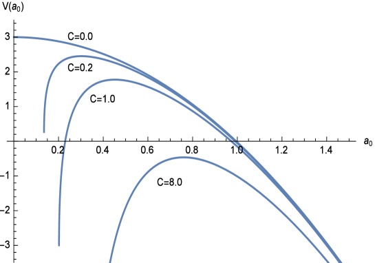
Fig. 1: Effective potential for $R=1.0,~{}\Lambda_{4}/3=1.0,~{}k=1,~{}\tilde{\alpha}^{2}=0.01$.

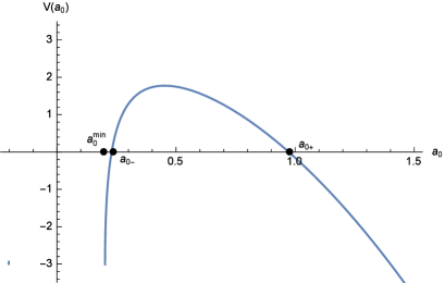
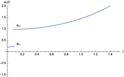
Fig. 2: Left: Potential barrier of $C=1.0$. Right: Two independent classical solutions for $a_{0}(t)$.

In the region $a_{0}^{\mathrm{min}}<a_{0}<a_{0-}$ (see the left panel of Fig. 2 again), there is a classical solution, but the solution does not provide the inflationary one. On the other hand, in the region $a_{0}>a_{0+}$, we obtain the inflationary solution. These two solutions are not connected to each other at the classical level. But they can be connected at the quantum level through the tunneling effect. See the right hand figure of Fig. 2. In [7], a new hilltop inflation scenario has been studied by using the Euclidean time solution (instanton) for this region.

(c) For $C\geq\frac{16\tilde{\alpha}^{2}\Lambda_{4}}{3}k^{2}R^{2}(1-4\tilde{\alpha}^{2}\frac{\Lambda_{4}}{3})$, there is no potential barrier and the classical inflationary solution is obtained for $a_{0}^{\rm min}<a_{0}$.

In the following sections, we consider the time evolution of the universe in the small $a_{0}$ region by using quantum cosmological approaches.

3 Quantum Cosmology and Effective Action

There are two quantum mechanical ways to study the small $a_{0}$ region, canonical approach and path-integral approach. In any case, we need an effective action which leads to the classical equations of motion (2.2) for an appropriate coordinate. It would be impossible to find a general coordinate invariant form since $\langle T_{\mu\nu}^{\mathrm{SYM}}\rangle$ comes from the conformal anomaly for the CFT.

However, we could find an effective action which provide the classical equations of motion, (2.5) and (2.6), written in the FRW metric. Namely, when the dynamical variable is restricted to the scale factor with a lapse function as a multiplier, it becomes possible to extend the analysis to the quantum cosmology.

Then we restrict ourselves in mini-superspace. Let us consider the metric

$$ds_{(4)}^{2}=-{\cal N}^{2}(t)dt^{2}+a_{0}(t)^{2}\gamma_{ij}dx^{i}dx^{j}\,,$$ (3.1)

where ${\cal N}(t)$ denotes the lapse function. According to the idea of [4, 8], the effective action is written as follows:

$$S = \int\!\!d^{4}x\sqrt{-g}\left\{{1\over 2\kappa_{4}^{2}}\left(R_{4}-{2}\Lambda_{4}\right)+L_{\mathrm{SYM}}^{\mathrm{eff}}\right\}\,$$ (3.2)

$$= V_{3}\!\!\int\!\!dt\,{\cal N}a_{0}^{3}\left\{{1\over\kappa_{4}^{2}}\left({3\over a_{0}^{2}}(-{\dot{a}_{0}^{2}\over{\cal N}^{2}}+k)-\Lambda_{4}\right)+L_{\mathrm{SYM}}^{\mathrm{eff}}\right\}\,,$$

where

$$L_{\mathrm{SYM}}^{\mathrm{eff}}=-{3N^{2}\over 32\pi^{2}}\left(\frac{4C}{R^{2}a_{0}^{4}}+{k^{2}\over a_{0}^{4}}-{2k\over a_{0}^{2}}{\dot{a}_{0}^{2}\over{\cal N}^{2}a_{0}^{2}}-{1\over 3{\cal N}^{4}}{\dot{a}_{0}^{4}\over a_{0}^{4}}\right)\,.$$ (3.3)

The Lagrangian $L_{\mathrm{SYM}}^{\mathrm{eff}}$ is determined such that we could find the Friedmann equation (2.5) from the stationary condition for ${\cal N}$ with ${\cal N}=1$ gauge. We should notice that (2.6) is also found from the variational equation of $a_{0}$. In this sense, (3.2) with (3.3) leads to a correct form of equations of motion to obtain our classical solutions. It is however difficult to develop an effective quantum theory based upon the action (3.2) due to the term (3.3). The situation is similar to the case with higher curvature terms.

Then we consider an alternative effective action which leads to (2.15) instead of (2.5). It is given as

$$S = \int\!\!d^{4}x\sqrt{-g}{1\over 2\kappa_{4}^{2}}\left(R_{4}-2\Lambda_{\rm eff}\right)\,$$ (3.4)

$$= V_{3}\!\!\int\!\!dt\,{\cal N}a_{0}^{3}{1\over\kappa_{4}^{2}}\left({3\over a_{0}^{2}}(-{\dot{a}_{0}^{2}\over{\cal N}^{2}}+k)-\Lambda_{\rm eff}\right)\,,$$

where

$$\Lambda_{\rm eff}^{\pm}=3\lambda_{\pm}\equiv 3\,{1\pm\sqrt{1-4\tilde{\alpha}^{2}\left(\frac{\Lambda_{4}}{3}+\tilde{\alpha}^{2}\frac{4}{R^{2}}\frac{C}{a_{0}^{4}}\right)}\over 2\tilde{\alpha}^{2}}\ .$$ (3.5)

This action is useful to perform the canonical formulation. In fact, from this action, it is easy to obtain the WDW equation (see Appendix A) which is not written here since we change the variable from $a_{0}$ to $q=a_{0}^{2}$.

3.1 Change of Variables

According to [14, 15], $a_{0}$ and ${\cal N}$ are changed as $q=a_{0}^{2}$ and ${\cal N}\rightarrow{\cal N}/a_{0}$, then we have

$$S = {V_{3}\over\kappa_{4}^{2}}\int\!\!dt\left(-{3\dot{q}^{2}\over 4\mathcal{N}}+\mathcal{N}(3k-q\Lambda_{\mathrm{eff}})\right)\,\ ,$$ (3.6)

$$\Lambda_{\mathrm{eff}} = 3\,\frac{~{}~{}1-\sqrt{1-4\tilde{\alpha}^{2}\left(\frac{\Lambda_{4}}{3}+\tilde{\alpha}^{2}\frac{4}{R^{2}}\frac{C}{q^{2}}\right)}~{}~{}}{2\tilde{\alpha}^{2}}\ .$$ (3.7)

In this formulation, the WDW equation is given as

$$\left(-\hbar^{2}\frac{\partial^{2}}{\partial q^{2}}+V(q)\right)\,\Psi(q)=0\ ,$$ (3.8)

which is also obtained by changing the variable as $q=a_{0}^{2}$ in (A.12), The potential $V(q)$ is given by

$$V_{\mathrm{eff}}(q)\equiv V(q)/(3v_{3}^{2})=3k-q\Lambda_{\mathrm{eff}}(q)\ .$$ (3.9)

3.2 $V_{\rm eff}(q)$ and tunneling

As shown in Sec. 2, we find similar behavior of the potential $V_{\rm eff}(q)$ to the case of $V(a_{0})$. The typical potentials are similar to Fig. 1, so they are abbreviated here.

Here we should notice as mentioned in Sec. 2 that there is a lower bound of $q$ for $C>0$. It corresponds to $a_{0}^{\rm nin}$ given in the previous section. The bound is given as

$$q^{\mathrm{min}}=\tilde{\alpha}^{2}\left({16C\over R^{2}\tilde{\Lambda}_{4}}\right)^{1/2}\,,\quad\tilde{\Lambda}_{4}=1-\frac{4\tilde{\alpha}^{2}\Lambda_{4}}{3}\,.$$ (3.10)

For $q<q^{\mathrm{min}}$, the potential becomes complex. So we cannot extend our model in this region. Therefore we concentrate our analysis on the region $q>q^{\mathrm{min}}$.

In this allowed region, several types of potentials are seen depending on the value of $C$. Hereafter we study the case shown in Fig. 3. This has two turning points, say $q_{-}$, and $q_{+}(>q_{-})$, in the two classical regions. For very small $C$, small sized universes may be made but they will soon disappear into the region of $q<q^{\mathrm{min}}$ where Einstein-Hilbert action is not available. However some of them would go through the mountain of the potential via a quantum tunneling effect. From the viewpoint of inflational scenario, this quantum jump of a small sized universe would give us a clue to the initial condition of the inflation.

Then, by using this potential, the tunneling birth of our universe can be studied.

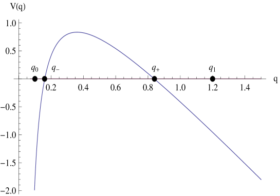
Fig. 3: Plots of $V_{\mathrm{eff}}(q)$ vs $q$ for $\Lambda_{4}=3,~{}k=1,~{}\tilde{\alpha}^{2}=0.01$ and $C=31.3$.

In principle, it is possible to calculate the propagator, $G(q_{1},q_{0})$ where the points $q_{0}$ and $q_{1}$ are shown in Fig. 3, according to the path-integral as discussed above in order to see the tunneling effect. However, it is difficult to find a saddle points in the complex ${\cal N}$ plane in the present model. So we perform the same calculation in terms of solving the WDW equation as given follows.

4 WDW equation and tunneling

Considering the potential as shown in Fig. 3, we give the tunneling amplitude for $C>0$ by solving the WDW equation (3.8). Supposing the form of the wave-function $\Psi(q)$ as follows:

$$\Psi(q)=A(q)e^{i\phi(q)/\hbar}\,,$$ (4.1)

the WDW equation (3.8) leads to the following equations,

$$(\partial_{q}\phi)^{2}+12\pi^{4}{V_{\rm eff}} = {\hbar^{2}\over A}\partial_{q}^{2}A\,,$$ (4.2)

$$\partial_{q}A\partial_{q}\phi+{1\over 2}A\partial_{q}^{2}\phi = 0\,.$$ (4.3)

They are solved by expanding $\phi$ with the power of $\hbar$.

In the regions of $q<q_{-}$ and $q_{+}<q$, the wave functions $\Psi_{1}$ and $\Psi_{3}$ are obtained in the following forms

$$\Psi_{1} = {c_{+}\over\sqrt{k(q)}}e^{-i\eta(q,~{}q_{-})}+{c_{-}\over\sqrt{k(q)}}e^{i\eta(q,~{}q_{-})}\,,$$ (4.4)

$$\Psi_{3} = {D_{+}\over\sqrt{k(q)}}e^{-i\eta(q_{+},~{}q)}+{D_{-}\over\sqrt{k(q)}}e^{i\eta(q_{+},~{}q)}\,,$$ (4.5)

where both the first terms of $\Psi_{1}$ and $\Psi_{3}$ represent the outgoing (growing) wave, and

$$k(q)=\sqrt{|V|}/\hbar\,,\quad\eta(q,~{}q_{-})=\int_{q}^{q_{-}}dq^{\prime}k(q^{\prime})\,,$$ (4.6)

where we notice that $\eta(q,~{}q_{-})=P(q,~{}q_{-})$ which is defined in the next section to express the Green function $G(q,~{}q_{-})$.

We can set various boundary conditions for the solutions of the wave-function $\Psi_{q}$. At first, we concentrate on the tunneling. In order to see the tunneling amplitude, we impose the condition $D_{-}=0$. Namely only the outgoing wave is restricted in the region $q_{+}<q$, then we find

$$D_{+}=c_{+}/\left({1\over 4}e^{-\eta(q_{-},~{}q_{+})}+e^{\eta(q_{-},~{}q_{+})}\right)\ .$$ (4.7)

Then we find the tunneling probability

$$T\simeq\left|{D_{+}\over c_{+}}\right|^{2}=e^{-2P(q_{+},q_{-})}\,.$$ (4.8)

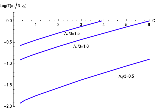
Fig. 4: Large $C$ dependence of the tunneling probability $T$ for different values of $\Lambda_{4}$

We expect that this result could also be found from the propagator given by the path-integral discussed above[14].

On the other hand, for the condition $D_{+}=-iD_{-}$, we find the relation

$$c_{+}={D_{+}\over 2}e^{-\eta(q_{-},~{}q_{+})}\,.$$ (4.9)

This leads to

$$\left|{D_{+}\over c_{+}}\right|^{2}=4\,e^{2P(q_{+},q_{-})}\,.$$ (4.10)

The sign of the exponent of $\left|{D_{+}\over c_{+}}\right|^{2}$ in this case is opposite to the tunneling case. This result corresponds to the one obtained in [21] as the wave-function of the WDW equation.

There are many other conditions, which lead to various forms of $\left|{D_{+}\over c_{+}}\right|^{2}$. The point we want to see is how these solutions of the WDW equation are related to the results of the path-integral. The saddle points given from the effective action of complex ${\cal N}$ can be related to the above solutions of the WDW equation. In order to answer to this question, we consider a simple model which has the properties of the above holographic model for $C>0$ case.

5 Quantum cosmology with Lorentzian path-integral

In the previous section, we considered canonical formalism to find the wave function of the universe by the WDW equation. In this section, let us consider the path-integral formalism to get the propagator of the universe.

The Feynman propagator in mini-superspace is defined as [14]

$$G(q_{1},q_{0})=\int_{0^{+}}^{\infty}d{\cal N}\int_{q_{0}}^{q_{1}}Dqe^{iS({\cal N},q)/\hbar}\,,$$ (5.1)

where $q_{0}=q(0)$ and $q_{1}=q(t_{1})$ are the initial and final values of $q(t)$. After integrating over $q$, we are left with the integration over ${\cal N}$. In order to perform the integration, we here try to apply the Lefschetz thimble method. In the Appendix C, the detail of this method is shown.

In this method, the original path is extended to the complex plane,

$${\cal N}=u_{1}+iu_{2}\ ,$$ (5.2)

where both $u_{1}=\mathrm{Re}\,({\cal N})$ and $u_{2}=\mathrm{Im}\,({\cal N})$ are real, and the propagator is evaluated by the saddle point approximation in the $\hbar\rightarrow 0$ limit. Below we shall see those examples concretely.

5.1 The case of $C=0$

In this case, the action (3.4) is equivalent to the one with the Einstein-Hilbert term and a cosmological constant. So, it has been already studied in [14]. Equation of motion for $q(t)$ and the constraint from (3.6) are

$$\ddot{q} = {2\over 3}\mathcal{N}^{2}\Lambda_{\mathrm{eff}},$$ (5.3)

$${3\dot{q}^{2}\over 4\mathcal{N}^{2}}+3k = q\Lambda_{\mathrm{eff}}\ .$$ (5.4)

The path integral over $q$ becomes Gaussian and is exactly treated. Then we are left with the integral over ${\cal N}$ as follows:

$$G(q_{1},q_{0})=\sqrt{\frac{3\pi i}{2\hbar}}\int_{0}^{\infty}\frac{d{\cal N}}{{\cal N}^{1/2}}e^{2\pi^{2}iS({\cal N})},$$ (5.5)

where

$$S({\cal N})=\frac{1}{36}{\cal N}^{2}\Lambda_{\mathrm{eff}}^{2}+\left(3k-\frac{1}{2}(q_{0}+q_{1})\right){\cal N}-\frac{3}{4{\cal N}}(q_{1}-q_{0})^{2}.$$ (5.6)

The action (5.6) has four saddle points in the complex ${\cal N}$ plane. If we choose, for instance, $k=1,\ \Lambda_{\mathrm{eff}}=3,\ q_{0}=0$ and $q_{1}=10$, those points lie at $(3,\ i),\ (3,-i),\ (-3,i)$ and $(-3,-i)$. Then, by using the thimble decomposition (as described in the Appendix C), it is found that the original contour is deformed to the Lefschetz thimble $J_{1}$ so that only one saddle ${\cal N}_{1}=(3,\ i)$ contributes to the integral (see Fig. 5).

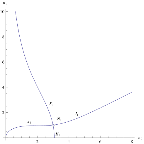
Fig. 5: Plots of Lefschetz thimble $J_{1}$ (the steepest descent) and $K_{1}$ (the steepest ascent) for the saddle $\mathcal{N}_{1}=(3,~{}i)$, where $\Lambda_{\mathrm{eff}}=3$, $k=1$, $q_{0}=0$, $q_{1}=10$.

The propagator obtained in this way is interpreted as the tunneling probability factor when the initial value $q_{0}$ is in the quantum region and the final point is at the zero point of $V_{\rm eff}$. It is given by

$$G(q_{1},q_{0})\propto e^{-2P(q_{1},q_{0})}\,,$$ (5.7)

where

$$P(q_{1},q_{0})={v_{3}\over\hbar}\int_{q_{0}}^{q_{1}}\!\!\sqrt{3V_{\rm eff}^{(0)}(q)}\,dq\ ,\quad V_{\rm eff}^{(0)}(q)=3k-q\Lambda_{\mathrm{eff}}^{(C=0)}(q)\,.$$ (5.8)

Here the oscillating part is abbreviated. This term precisely denotes the tunneling probability found in the WKB approximation of the WDW equation in the previous section.

Here is a comment. In this case, we find other three saddle points which do not contribute to the integration. However, they might affect in some case where the integration path is defined in a different way[21].

The tunneling factor (5.8) appears whenever either $q_{0}$ or $q_{1}$ is in the quantum region. So the Lefschetz thimble method is useful to study quantum cosmology and it is equivalent to solve the WDW equation under appropriate boundary conditions.

5.2 The case of $C\neq 0$

It is difficult to perform the path-integral for the potential $V_{\rm eff}(q)$ with $C\neq 0$ due to a complicated $q$-dependence of $V_{\rm eff}(q)$. Then let us consider the following action, that is,

$$S = {v_{3}}\!\int\!dt\left(-{3\dot{q}^{2}\over 4{\cal N}}+{\cal N}(3k-\mu(q_{c}-q)^{2}-\beta)\right)\,\qquad(\mu>0)\ .$$ (5.9)

Here the original $V_{\mathrm{eff}}(q)$ defined by (3.9) is approximated by a quadratic form near its maximum point, $q_{c}$.

By doing this, one can study the model analytically without losing characteristic properties of the original model within the approximation mentioned above. Then we use the following potential $V_{\mathrm{sim}}$ (see Fig. 6):

$$V_{\mathrm{sim}}\equiv 3k-\mu(q_{c}-q)^{2}-\beta\ ,$$ (5.10)

where $\mu$ and $\beta$ are constant parameters. Hereafter we discuss the case of $\beta=0$.

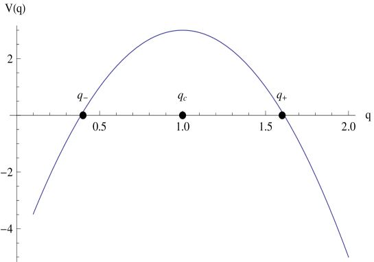
Fig. 6: Plots of $V_{\mathrm{sim}}=V(q)$, the simplified model (5.10), for $q_{c}=1$, $\mu=8$, and $k=1$. $q_{\pm}$ denote the zero points of $V(q)$.

Equation of motion for $q$ is easily solved as

$$q=q_{c}+a_{+}e^{\frac{{\cal N}}{t_{0}}t}+a_{-}e^{-\frac{{\cal N}}{t_{0}}t}\,,\quad t_{0}\equiv\sqrt{{3\over 4\mu}}\ .$$ (5.11)

The coefficients $a_{\pm}$ are determined through the boundary conditions, $q(0)=q_{0}$ and $q(1)=q_{1}$:

$$a_{+} = -{\tilde{q}_{0}e^{-\frac{{\cal N}}{t_{0}}}-\tilde{q}_{1}\over 2\sinh(\frac{{\cal N}}{t_{0}})}\,,$$ (5.12)

$$a_{-} = {\tilde{q}_{0}e^{\frac{{\cal N}}{t_{0}}}-\tilde{q}_{1}\over 2\sinh(\frac{{\cal N}}{t_{0}})}\,,$$ (5.13)

$$\tilde{q}_{i} \equiv q_{i}-q_{c}\ .$$ (5.14)

By substituting these coefficients into (5.9), we get

$$S_{\mathrm{sim}}^{(0)}=v_{3}\mu t_{0}\left({3k{\cal N}\over\mu t_{0}}-{(\tilde{q}_{1}^{2}+\tilde{q}_{0}^{2})\cosh(\frac{{\cal N}}{t_{0}})-2\tilde{q}_{1}\tilde{q}_{0}\over\sinh(\frac{{\cal N}}{t_{0}})}\right)\ .$$ (5.15)

From the stationary condition $\delta S_{\mathrm{sim}}^{(0)}/\delta{\cal N}=0$, we find two saddle points, say ${\cal N_{\pm}}$:

$${\cal N_{\pm}}=t_{0}\cosh^{-1}\left\{{\mu\over 3k}\left(\tilde{q}_{0}\tilde{q}_{1}\pm\sqrt{\left(\tilde{q}_{0}^{2}-{3k\over\mu}\right)\left(\tilde{q}_{1}^{2}-{3k\over\mu}\right)}\right)\right\}.$$ (5.16)

In order to solve (5.16), we parameterize ${\cal N}$ in the polar coordinate $(r,\ \theta)$:

$$e^{\frac{{\cal N}}{t_{0}}}=re^{i\theta}\,\quad{\rm or}\quad{\cal N}=(\log r+i~{}\theta)t_{0}\ .$$ (5.17)

Then (5.16) can be rewritten in terms of $r$ and $\theta$:

$$\cosh\left(\frac{{\cal N}}{t_{0}}\right) = {1\over 2}\left[\left(r+{1\over r}\right)\cos\theta+i\left(r-{1\over r}\right)\sin\theta\right]\,$$ (5.18)

$$= Q_{0}Q_{1}\pm\sqrt{(Q_{0}^{2}-1)(Q_{1}^{2}-1)}\,\equiv X_{\pm},$$

where

$$Q_{0}={\tilde{q}_{0}\over|\tilde{q}_{\pm}|}\,,\quad Q_{1}={\tilde{q}_{1}\over|\tilde{q}_{\pm}|}\,,\quad\tilde{q}_{\pm}=\pm\sqrt{{3k\over\mu}}\ .$$ (5.19)

Note that $\tilde{q}_{\pm}$ denote the zeroes of the potential term $V_{\mathrm{sim}}$ defined by (5.10).

5.2.1 Tunneling

Let us consider a situation that $q_{0}$ and $q_{1}$ are put on the opposite side of the hill of the potential (see Fig. 7). The transition from $q_{0}$ to $q_{1}$ would be realized by the quantum tunneling.

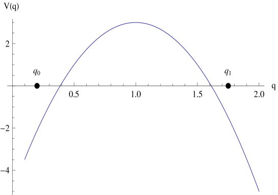
Fig. 7: Plots of the typical position of $q_{0}$ and $q_{1}$ for the tunneling process are shown with $V_{\mathrm{sim}}=V(q)$, the simplified model (5.10) shown in Fig. 6.

In this case, since $Q_{0}<-1$ and $Q_{1}>1$, $X_{\pm}$ in (5.18) are real and satisfy an inequality $X_{-}<X_{+}<-1$. Then we obtain

$$X_{\pm} = -{1\over 2}\left(r_{\pm}+{1\over r_{\pm}}\right)(<-1)\,,$$ (5.20)

$$\theta = \pm(2n+1)\pi\,,\quad n=0,\pm 1,\pm 2,\ldots$$ (5.21)

From this, we find two values of $r$, at $r_{\pm l}>1$ and $r_{\pm s}<1$, for $X_{\pm}$. So there are eight saddle points for one $|\theta|$ in the complex ${\cal N}$ plane. In Fig. 8, saddle points for $n=0$ with some specific parameters are shown.

Fig. 8: Plots of the saddle point of ${\cal N}$ for the simplified model. Here the case of $\theta=\pi$, $\tilde{q}_{0}=-\tilde{q}_{+}(1+0.2)$ and $\tilde{q}_{1}=\tilde{q}_{+}(1+0.5)$ is shown.

We should notice that there are no real ${\cal N}$ solutions in the present case. This implies that the path connecting $q_{0}$ and $q_{1}$ represents a quantum process.

For the saddle points with $\theta=\pi~{}~{}(n=0)$ and $r=r_{\pm s}$, the action is evaluated as

$$\mathrm{Re}\,\left[{2\pi^{2}\over\hbar}iS_{0}\right] = -{2\pi^{2}\over\hbar}{3\pi t_{0}}=-{3\sqrt{3}\pi^{3}\over\sqrt{\mu}\hbar}$$ (5.22)

$$= -{\sqrt{12}\pi^{2}\over\hbar}\int_{\tilde{q}_{-}}^{\tilde{q}_{+}}\sqrt{3k-\mu\tilde{q}^{2}}d\tilde{q}=-P(\tilde{q}_{+},\tilde{q}_{-}).$$

Then the factor $e^{-P(\tilde{q}_{+},\tilde{q}_{-})}$ corresponds to the tunneling amplitude.

As for the above solution, the propagator has a slightly different phase from the one of $r=r_{\pm s}$. This implies that this solution corresponds to the propagator traveling a slightly long path in the classical region $0<q<q_{-}$.

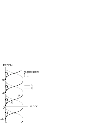
Fig. 9: A sketch of the thimbles: Due to the degeneracy between steepest descent and ascent flows (thimbles and dual thimbles), it is not possible to classify the flow segments, definitely. For each saddle point on the relevant integration path, a neighboring segment of a steepest descent flow is labeled with $J_{i}$ and one of a steepest ascent flow is with $K_{i}$.

The propagator is calculated by integrating the r. h. s. of (5.1) over $q$, and the integration path of $\mathcal{N}$ is deformed to a curve in the first quadrant of the complex $\mathcal{N}$ plane. In the method of the Lefschetz thimble, the curved path contains some steepest descent flows of $\mathrm{Re}\,[i{S^{(0)}_{\mathrm{min}}(\mathcal{N})}]$. As shown in Fig. 9, there are two possible saddle points each of which connects to the origin $\mathcal{N}=0$ through a steepest descent flow (a Lefschetz thimble). One is $\mathcal{N}_{p}^{(n=0)}=(-\cosh^{-1}(-Q_{0})+\cosh^{-1}Q_{1}+i\pi)t_{0}$ in the $\mathcal{N}_{p}$ series and another is $\mathcal{N}_{m}^{(n=0)}=(\cosh^{-1}(-Q_{0})+\cosh^{-1}Q_{1}+i\pi)t_{0}$ in the $\mathcal{N}_{m}$ series.

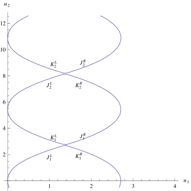
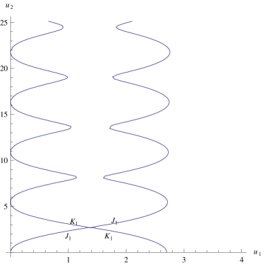
Fig. 10: Left: Plots of the Lefschetz thimbles for ${\cal N}_{m}$ of the simplified model. Here the case of $\theta=\pi$, $\tilde{q}_{0}=-\tilde{q}_{+}(1+0.2)$ and $\tilde{q}_{1}=\tilde{q}_{+}(1+0.5)$ is shown. Right: The thimbles corresponding to the first saddle of ${\cal N}_{m}$ series or an integral path when a perturbation $\Delta S_{0}=i{\cal N}/100.$ is included.

The thimble which passes the former saddle point $\mathcal{N}_{p}^{(n=0)}$ connects to the singular point at $\mathcal{N}=i(\pi+0)t_{0}$, and is terminated there. This means that the thimble attached to this saddle point is irrelevant to the present method. On the other hand, the thimble which passes the latter saddle point $\mathcal{N}_{m}^{(n=0)}$ does not reach any singular point before the next saddle point $\mathcal{N}_{m}^{(n=1)}=(\cosh^{-1}(-Q_{0})+\cosh^{-1}Q_{1}+3i\pi)t_{0}$. This thimble is shown as the set of $J_{1}^{L}$ and $J_{1}^{R}$ in Fig. 9 and also in the left panel of Fig. 10. Furthermore, its dual thimble (the steepest ascent flow) intersects the real axis of the complex $\mathcal{N}$ plane. Therefore, the relevant path should run from the origin toward the saddle point $\mathcal{N}_{m}^{(n=0)}$. Now, the Lefschetz thimbles are obtained as the flow lines emanating from the saddle points of the $\mathcal{N}_{m}$ series, as shown in the left of Fig. 10.

However, the situation is somewhat complicated because of the degeneracy between the flow lines $J_{i}$ and $K_{i+1}$ . To find the appropriate path over the saddle point $\mathcal{N}_{m}^{(n=1)}$, one may try to provide a perturbation term to the original action (5.15), for example, $\Delta S_{0}=i{\cal N}/100$. Actually, $\Delta S_{0}$ removes the degeneracy as depicted by the right panel of Fig. 10. Finally, setting $\Delta S_{0}=0$ again, one finds a unique path as $J_{1}^{L}\rightarrow J_{1}^{R}\rightarrow K_{2}^{R}\rightarrow J_{2}^{R}\rightarrow\cdots$ , where only the first saddle point $\mathcal{N}_{m}^{(n=0)}$ dominates the integration.

Tunneling probability via steepest descent method

The tunneling probability is estimated by using the propagator (5.1), and in the simplified model the amplitude is reduced to

$$G(q_{1},q_{0})=\int_{0^{+}}^{\infty}\!\!\sqrt{\frac{3i/2t_{0}}{2\pi\sinh(\frac{{\cal N}}{t_{0}})}}\,\,e^{iS_{\mathrm{sim}}^{(0)}(\mathcal{N})}\,d\mathcal{N}$$ (5.23)

after integrating over $q$.

As mentioned above, $G(q_{1},q_{0})$ is approximately evaluated by the main contribution of the saddle point at

$$\mathcal{N}_{0}\equiv\mathcal{N}_{m}^{(n=0)}=(\cosh^{-1}(-Q_{0})+\cosh^{-1}Q_{1}+i\pi)\,t_{0}\ ,$$ (5.24)

which is the joint of $J_{1}^{L}$ and $J_{1}^{R}$. Then, the amplitude (5.23) is calculated as follows:

$$G(q_{1},q_{0}) \simeq \sqrt{\frac{3i/2t_{0}}{2\pi\sinh(\frac{{\cal N}}{t_{0}})}}\,\,\,e^{i\mathrm{Re}\,S_{\mathrm{sim}}^{(0)}(\mathcal{N}_{0})}\!\!\mathop{\int}_{J_{1}^{L}+J_{1}^{R}}\!\!\!e^{-\mathrm{Im}\,S_{\mathrm{sim}}^{(0)}(\mathcal{N})}\,d\mathcal{N}$$ (5.25)

$$\simeq \sqrt{\frac{3i/2t_{0}}{2\pi\sinh(\frac{{\cal N}}{t_{0}})}}\,e^{i\mathrm{Re}\,S_{\mathrm{sim}}^{(0)}(\mathcal{N}_{0})}\!\!\int_{-\infty}^{\infty}\!\!\!\!e^{-\mathrm{Im}\,S_{\mathrm{sim}}^{(0)}(\mathcal{N}_{0})-\frac{1}{2}|S_{\mathrm{sim}}^{(0)}{}^{\prime\prime}(\mathcal{N}_{0})|\nu^{2}}e^{i\theta_{0}}d\nu$$ (5.26)

$$= \sqrt{\frac{3i/2t_{0}}{2\pi\sinh(\frac{{\cal N}}{t_{0}})}}\,e^{i(\mathrm{Re}\,S_{\mathrm{sim}}^{(0)}(\mathcal{N}_{0})+\theta_{0})}e^{-\mathrm{Im}\,S_{\mathrm{sim}}^{(0)}(\mathcal{N}_{0})}\,\sqrt{\frac{2\pi}{|S_{\mathrm{sim}}^{(0)}{}^{\prime\prime}(\mathcal{N}_{0})|}}\ ,$$ (5.27)

where $\theta_{0}$ is the incident angle of the thimble $J_{1}^{L}$ into the point $\mathcal{N}_{0}$ in the complex $\mathcal{N}$ plane. The angle $\theta_{0}$ is determined by

$$\tan\theta_{0}=\frac{\mathrm{Re}\,S_{\mathrm{sim}}^{(0)}{}^{\prime\prime}(\mathcal{N}_{0})}{|S_{\mathrm{sim}}^{(0)}{}^{\prime\prime}(\mathcal{N}_{0})|+\mathrm{Im}\,S_{\mathrm{sim}}^{(0)}{}^{\prime\prime}(\mathcal{N}_{0})}=\frac{|S_{\mathrm{sim}}^{(0)}{}^{\prime\prime}(\mathcal{N}_{0})|-\mathrm{Im}\,S_{\mathrm{sim}}^{(0)}{}^{\prime\prime}(\mathcal{N}_{0})}{\mathrm{Re}\,S_{\mathrm{sim}}^{(0)}{}^{\prime\prime}(\mathcal{N}_{0})}\ .$$ (5.28)

Since it holds that

$$S_{\mathrm{sim}}^{(0)}{}^{\prime\prime}(\mathcal{N})=\frac{3v_{3}k}{t_{0}}\,F^{(2)}\left(\frac{{\cal N}}{t_{0}}\right)$$ (5.29)

with

$$F^{(2)}\left(\frac{{\cal N}}{t_{0}}\right)=\left[\frac{2Q_{0}Q_{1}\cosh^{2}(\frac{{\cal N}}{t_{0}})-2(Q_{0}^{2}+Q_{1}^{2})\cosh(\frac{{\cal N}}{t_{0}})+2Q_{0}Q_{1}}{\sinh^{3}(\frac{{\cal N}}{t_{0}})}\right]\ ,$$ (5.30)

the second order derivative $S_{\mathrm{sim}}^{(0)}{}^{\prime\prime}(\mathcal{N})$ satisfies that

$$\mathrm{Re}\,S_{\mathrm{sim}}^{(0)}{}^{\prime\prime}(\mathcal{N}_{0})>0\ ,\quad\mathrm{Im}\,S_{\mathrm{sim}}^{(0)}{}^{\prime\prime}(\mathcal{N}_{0})=0\ .$$ (5.31)

Therefore, the angle $\theta_{0}$ is found to be $\frac{\pi}{4}$.

Now, the absolute value of the tunneling amplitude is given by

$$|G(q_{1},q_{0})| = \sqrt{\frac{3/2t_{0}}{|\sinh(\frac{{\cal N}}{t_{0}})\,S_{\mathrm{sim}}^{(0)}{}^{\prime\prime}(\mathcal{N}_{0})|}}\,e^{-\mathrm{Im}\,S_{\mathrm{sim}}^{(0)}(\mathcal{N}_{0})}$$ (5.32)

$$= \sqrt{\frac{1}{2v_{3}k|\sinh(\frac{{\cal N}}{t_{0}})\,F^{(2)}(\frac{{\cal N}}{t_{0}})|}}\,e^{-\mathrm{Im}\,S_{\mathrm{sim}}^{(0)}(\mathcal{N}_{0})}\ ,$$ (5.33)

in which the factor $|\sinh(\mathcal{N}_{0}/t_{0})\,F^{(2)}(\mathcal{N}_{0}/t_{0})|$ is a certain function of $Q_{0}$ and $Q_{1}$, and

$$-\mathrm{Im}\,S_{\mathrm{sim}}^{(0)}(\mathcal{N}_{0})=-3kv_{3}t_{0}\pi\ .$$ (5.34)

We can see $\mathrm{Im}\,S_{\mathrm{sim}}^{(0)}(\mathcal{N}_{0})=P(q_{+},q_{-})$, where $P(q_{+},q_{-})$ is defined by (4.6) in Sec. 4 when $V$ is replaced by the simplified potential $V_{\rm sim}$ used in the present section. This implies the result obtained here reproduces the tunneling probability $e^{-2P(q_{+},q_{-})}$ given in Sec. 4. From Eq. (5.33), it is found that $|G(q_{1},q_{0})|^{2}$ depends on $t_{0}$ such as

$$|G(q_{1},q_{0})|^{2}\propto e^{-6kv_{3}t_{0}\pi}\ .$$ (5.35)

5.2.2 Saddles for periodic Euclidean solution

In the previous subsection, we considered the saddle-point contribution from the $n=0$ sector. Then a natural question arises: What is the meaning of other infinite series of the saddle points for $n\geq 1$? We could answer to the question by considering the “instanton”[7]. In [7], the authors have found a periodic Euclidean solution of the Friedmann equation regarded as an instanton one, which oscillates between $q_{-}$ and $q_{+}$.

In the following, let us estimate the instanton contribution by using the Euclidean path-integral formalism. In our simplified model with $V_{\mathrm{sim}}$, equations of motion for $q$ in the Euclidean time $\tau$ is given by

$$\left({\partial q\over\partial\tau}\right)^{2}=-{4\over 3}\mu(q-q_{c})^{2}+4k$$ (5.36)

Then the solution is easily obtained as

$$q_{I}=\sqrt{{3\over\mu}}\sin\left(\sqrt{{4\mu\over 3}}\right)+q_{0}=2t_{0}\sin\left(\frac{\tau}{t_{0}}\right)+q_{0}$$ (5.37)

The period of the solution, $T_{0}$, becomes

$$T_{0}=2\pi t_{0}=\pi\sqrt{\frac{3}{\mu}}\,.$$ (5.38)

Then we get the Euclidean action for the instanton solution:

$$S_{0}^{E} = iv_{3}\int_{0}^{T_{0}}d\tau\left({3\over 4}\dot{q}^{2}+3k-\mu(q-q_{c})^{2}\right)\,$$ (5.39)

$$= iv_{3}\times 3T_{0}\ .$$ (5.40)

Therefore, we find

$$\mathrm{Re}\,\left[{2\pi^{2}\over\hbar}\,iS_{0}^{E}\right]=-{2\pi^{2}\over\hbar}{6\pi t_{0}}=-{6\sqrt{3}\pi^{3}\over\sqrt{\mu}\hbar}=-2P(\tilde{q}_{+},\tilde{q}_{-})\ .$$ (5.41)

On the other hand, for the saddle point solutions corresponding to (5.21), we have

$$\mathrm{Re}\,\left[{2\pi^{2}\over\hbar}\,iS_{0}\right]=-(2n+1)P(\tilde{q}_{+},\tilde{q}_{-})\,.$$ (5.42)

From this result, we could say that the saddle contribution with $n\geq 1$ represents that from “$n$ instantons”. They are exponentially suppressed compared to the leading $n=0$ contribution. These saddle points for $n\geq 1$, however, do not contribute as saddles in the integral given above to evaluate the propagator due to the path which is chosen as the Lefschetz thimble of $n=0$ saddle point.

6 Summary and Discussions

In this paper, cosmology driven by SYM theory is studied in the FRW space-time. Here all the SYM fields are integrated out and the vacuum expectation value of its energy-momentum tensor $\langle T_{\mu\nu}^{\mathrm{SYM}}\rangle$ is given by holographic method. Based on the equations of motion with this $\langle T_{\mu\nu}^{\mathrm{SYM}}\rangle$, we introduced a new simple effective action which could reproduce the equations of motion of the theory.

The SYM theory provides two kinds of terms in the action, loop correction term and a radiation term. The gravitational part includes the 4D cosmological constant $\Lambda_{4}$. The value of $\Lambda_{4}$ is restricted to be positive in order to realize the inflationary universe at large scale factor $a_{0}$. In the present case, however, it is not completely free. When SYM theory is included, $\Lambda_{4}$ is bounded from above, so the expansion rate at large $a_{0}$ is modified by the loop correction of the SYM fields.

In the region of small $a_{0}$, the radiation plays an important role. Although the magnitude of the radiation is arbitrary, there appears a lower bound of $a_{0}$. Further, a small scale universe with the radiation could be born and appear at large $a_{0}$ after a quantum tunneling. Here, this phenomenon is studied through two quantum cosmological methods for mini-superspace of gravity.

One is to solve the WDW equation. Here the WDW equation is easily given by considering our effective action introduced as mentioned above. In this sense, our effective action is very useful to study the quantum mechanics of the theory. The tunneling probability is calculated by imposing an appropriate boundary condition at large $a_{0}$ for both cases of $C=0$ and $C>0$.

The other is to calculate the same quantity by Lorentzian path-integral according to the method proposed by [14]. This method is useful when the radiation is absent. The result coincides with the solution of the WDW equation.

On the other hand, it is difficult to proceed the calculation in terms of the effective action used for the WDW equation when the radiation exists. So we consider a simplified model in which the potential in the WDW equation is approximated by the harmonic form. In this case, we could show a Lefschetz thimble as the unique path for the tunneling propagator. The calculation is performed according to the steepest descent method, and the result coincides with the solution of the WDW equation with the same harmonic potential. We should notice that, for the harmonic potential, we have many saddle points in the complex lapse ${\cal N}$ plane. However, the path, which contributes to the Lorentzian path-integral, has only one saddle which corresponds to the tunneling.

Although, here, we concentrated to the tunneling amplitude, there are other kinds of propagators whose initial and final values of $a_{0}$ are different from the one of the tunneling case. The situation is also depending on the form of potential. It is characterized by the radiation and $\Lambda_{4}$. On such various kinds of propagators, we will discuss in the future.

Appendix A The Wheeler-DeWitt equation

At first, we give the Wheeler-DeWitt equation used to obtain the wave-function of the universe. (3.4) is written as

$$S=\int\!\!dt\,L$$ (A.1)

$$L=\mathcal{N}a_{0}^{3}\left(\frac{3}{a_{0}^{2}}\left(-\frac{\dot{a}_{0}^{2}}{\mathcal{N}^{2}}+k\right)-\Lambda_{\mathrm{eff}}\right)v_{3}\,,\quad v_{3}={V_{3}\over\kappa_{4}^{2}}$$ (A.2)

where

$$\Lambda_{\mathrm{eff}}=3\lambda_{-}=3\,\frac{~{}~{}1-\sqrt{1-4\tilde{\alpha}^{2}\left(\frac{\Lambda_{4}}{3}+\tilde{\alpha}^{2}\frac{4}{R^{2}}\frac{C}{a_{0}^{4}}\right)}~{}~{}}{2\tilde{\alpha}^{2}}$$ (A.3)

$$p_{a}=\frac{\partial L}{\partial\dot{a}_{0}}=-{6\over\mathcal{N}}a_{0}\dot{a}_{0}v_{3}$$ (A.4)

Then

$$H = p_{a}\dot{a}_{0}-L$$ (A.5)

$$= -\frac{\mathcal{N}}{12a_{0}v_{3}}\left(p_{a}^{2}+{12a_{0}^{4}v_{3}^{2}}\left(\frac{3}{a_{0}^{2}}k-\Lambda_{\mathrm{eff}}\right)\right)$$ (A.6)

$$= \mathcal{N}\hat{H}$$ (A.7)

where

$$\hat{H}=-\frac{1}{12a_{0}v_{3}}\left(p_{a}^{2}+{12a_{0}^{4}v_{3}^{2}}\left(\frac{3}{a_{0}^{2}}k-\Lambda_{\mathrm{eff}}\right)\right)$$ (A.8)

Then we have

$$S=\int dt~{}(p_{a}\dot{a}_{0}-\mathcal{N}\hat{H})$$ (A.9)

This indicates the lapse function $\mathcal{N}$ is a Lagrange multiplier providing the constraint

$$\hat{H}=0$$ (A.10)

This is written to a quantized form by using

$$p_{a}\rightarrow-i\frac{\partial}{\partial a_{0}}$$ (A.11)

as

$$\left(-\frac{\partial^{2}}{\partial a_{0}^{2}}+{12a_{0}^{2}v_{3}^{2}}\left(3k-a_{0}^{2}\Lambda_{\mathrm{eff}}\right)\right)\,\Psi(a_{0})=0$$ (A.12)

This equation could be applied to the region where a classical solution for $a_{0}(t)$ is forbidden. In the below, by changing the variable in this equation, we show some numerical result for the tunneling process under an appropriate boundary conditions.

Appendix B Derivation of Eq. (3.3)

The result (3.3) is obtained as follows. Assuming the form of $L_{\mathrm{SYM}}^{\mathrm{eff}}$ as,

$$L_{\mathrm{SYM}}^{\mathrm{eff}}=h_{0}(a_{0})+{\dot{a}_{0}^{2}\over{\cal N}^{2}}h_{2}(a_{0})+{\dot{a}_{0}^{4}\over{\cal N}^{4}}h_{4}(a_{0})\,.$$ (B.1)

This form would be supported by the analyticity and $g_{0i}=0$ gauge (3.1). By substituting this into (3.2), we find from $\delta S/\delta{\cal N}=0$,

$$\left\{{1\over\kappa_{4}^{2}}\left(3a_{0}({\dot{a}_{0}^{2}\over{\cal N}^{2}}+k)-a_{0}^{3}\Lambda_{4}\right)+a_{0}^{3}\left(h_{0}-{\dot{a}_{0}^{2}\over{\cal N}^{2}}h_{2}-3{\dot{a}_{0}^{4}\over{\cal N}^{4}}h_{4}\right)\right\}\delta{\cal N}=0$$ (B.2)

This is compared with (2.5) for ${\cal N}=1$ gauge,

$$\lambda\equiv\left({\dot{a}_{0}\over a_{0}}\right)^{2}+{k\over a_{0}^{2}}={\Lambda_{4}\over 3}+{\kappa_{4}^{2}\over 3}\langle T_{00}^{\mathrm{SYM}}\rangle\,,$$ (B.3)

where

$$T_{00}^{\mathrm{SYM}}=\rho={3\alpha\over 16}\left(\frac{4C}{R^{2}a_{0}^{4}}+\lambda^{2}\right)\,,\quad\lambda={\dot{a}_{0}^{2}\over a_{0}^{2}}+{k\over a_{0}^{2}}$$ (B.4)

Then we have,

$$h_{0} = -{3\alpha\over 16}\left(\frac{4C}{R^{2}a_{0}^{4}}+{k^{2}\over a_{0}^{4}}\right)\,,$$ (B.5)

$$h_{2} = {3\alpha\over 8}{k\over a_{0}^{4}}\,,$$ (B.6)

$$h_{4} = {\alpha\over 16}{1\over a_{0}^{4}}\,,$$ (B.7)

Plugging this into (B.1) we find (3.3), which is expressed for general ${\cal N}$.

Appendix C Picard-Lefschetz method

In this Appendix, let us introduce the Picard-Lefschetz method . In the path-integral formalism, the partition function is defined by

$$Z=\int_{\mathcal{M}}d\Phi\exp\left({\cal F}(\Phi)/\hbar\right),$$ (C.1)

where $\mathcal{M}$ is the target space of parameters $\Phi$. Since this integral is, in general, an multi-dimensional oscillatory integral, we need a technique to consider about it. Here we use the Lefschetz-thimble method [23][24].

The basic idea is to deform the integration contour $\mathcal{M}$ into steepest descent cycles inside its complexified space $\mathcal{M}_{\mathbb{C}}$ by using the Cauchy theorem when ${\cal F}$ is holomorphic. We denote the holomorphic coordinate of $\mathcal{M}_{\mathbb{C}}$ as $\Phi=(z^{1},\ldots,z^{n})$, and the set of saddle points as

$$\Sigma=\{z_{\sigma}\}:=\left\{\frac{\partial{\cal F}}{\partial z^{i}}=0\right\}.$$ (C.2)

Using the Kähler metric on $\mathcal{M}_{\mathbb{C}}$, $ds^{2}=g_{i\overline{j}}dz^{i}\otimes d\overline{z^{j}}$, we define the gradient flow by

$$\frac{dz^{i}}{dt}=g^{i\overline{j}}{\left(\frac{\partial\overline{{\cal F}}}{\partial\overline{z^{j}}}\right)}.$$ (C.3)

As an important property of this differential equation, we have

$${d{\cal F}\over dt}=\left|\partial{\cal F}\right|^{2}\geq 0.$$ (C.4)

Therefore, along the flow line, the real part of the free energy increases while its imaginary part stays constant. This means that we can define the steepest descent and ascent cycles associated with each saddle point $z_{\sigma}$ by this gradient flow. Using solutions of the gradient flow $z(t)$, they are defined as

$$\mathcal{J}_{\sigma}=\{z(0)\,|\,z(t)\to z_{\sigma},t\to-\infty\},\quad\mathcal{K}_{\sigma}=\{z(0)\,|\,z(t)\to z_{\sigma},t\to+\infty\}.$$ (C.5)

These are called Lefschetz thimbles and dual thimbles. They are dual quantities in terms of the intersection pairing $\langle\cdot,\cdot\rangle$, i.e., $\langle\mathcal{J}_{\sigma},\mathcal{K}_{\tau}\rangle=\delta_{\sigma\tau}$, which means that one can decompose $\mathcal{M}$ in terms of $\mathcal{J}_{\sigma}$ as

$$\int_{\mathcal{M}}d\Phi\exp\left({\cal F}(\Phi)/\hbar\right)=\sum_{\sigma\in\Sigma}\langle\mathcal{M},\mathcal{K}_{\sigma}\rangle\int_{\mathcal{J}_{\sigma}}d^{n}z\exp\left({\cal F}(\Phi)/\hbar\right).$$ (C.6)

If all $\mathrm{Re}({\cal F}(\Phi_{\sigma}))$ are different with each other in the limit $\hbar\to 0$, we replace the integral by the saddle-point approximation. Then we obtain at the leading order that

$$Z=\sum_{\sigma}\langle\mathcal{M},\mathcal{K}_{\sigma}\rangle\exp\left({\cal F}(z_{\sigma})/\hbar\right).$$ (C.7)

We can summarize the necessary steps of the mean-field approximation with the sign problem as follows:

1. Complexify the target space $\mathcal{M}$ to $\mathcal{M}_{\mathbb{C}}$, and find the saddle points $z_{\sigma}$ by solving the equation $\partial{\cal F}=0$ in $\mathcal{M}_{\mathbb{C}}$.

2. Solve the gradient flow (C.3), and construct Lefschetz thimbles $\mathcal{J}_{\sigma}$ and dual thimbles $\mathcal{K}_{\sigma}$.

3. Pick up the saddle point $z_{\sigma}$ that has the minimal free energy $\mathrm{Re}({\cal F}(z_{\sigma}))$ with nonzero intersection number $\langle\mathcal{M},\mathcal{K}_{\sigma}\rangle$.

References

[1]
K. Ghoroku M. Ishihara and A. Nakamura,
Phys. Rev. D74 124020 (2006).
K. Ghoroku M. Ishihara and A. Nakamura,
Phys. Rev. D75 046005 (2007).
[2] J. Erdmenger, K. Ghoroku and R. Meyer,
Phys. Rev. D84, 026004 (2011)
[arXiv:1105.1776 (hep-th)].
[3] J. Erdmenger, K. Ghoroku, R. Meyer and I. Papadimitriou,
Fortsch. Phys. 60 (2012) 991—997
[arXiv:1205.0677 (hep-th)].
[4] M. V. Fischetti, J. B. Hartle, and B. L. Hu, Phys. Rev.
D20, 1757 (1979).
[5] K. Ghoroku, R. Meyer and F. Toyoda,
Phys. Rev. D96, 086011 (2017) [arXiv:1706.07889].
[6] A. Awad,
Phys. Rev. D93, 084006 (2016)
[arXiv:1512.06405[hep-th]].
[7] A. O. Barvinsky, A. Yu. Kamenshchik and D.V. Nesterev
[arXiv:1510.06858[hep-th]].
[8]A. O. Barvinsky and A. Yu. Kamenshchik, JCAP 0609, 014 (2006);
Phys. Rev. D74, 121502 (2006).
[9] N. Bilic,
Phys. Rev. D93, 066010 (2016) [arXiv:1511.07323 [gr-qc]].
[10] P. Binetruy, C. Deffayet, U. Ellwanger and D. Langlois,
Phys. Lett. B477 285-291 (2000) [hep-th/9910219].
[11] D. Langlois,
Phys. Rev. D62 126012 (2000) [hep-th/0005025].
D. Langlois and L. Sorbo,
Phys. Rev. D68 084006 (2003) [hep-th/0306281].
[12] T. Shiromizu, K. Maeda and M. Sasaki,
Phys. Rev. D62, 024012 (2000) [gr-qc/9910076].
[13] M. Sasaki, T. Shiromizu and K. Maeda,
Phys. Rev. D62, 024008 (2000) [hep-th/9912233].
K. Maeda, S. Mizuno and T. Torii,
Phys. Rev. D68, 024033 (2003) [gr-qc/0303039].
[14] J. Feldbrugge, J.-L. Lehners and N. Turok,
Phys. Rev. D95, 103508 (2017) [arXiv:1703.02076].
[15] J. J. Halliwell and J. Louko, Phys. Rev. D39 (1989) 2206.
[16] J. Feldbrugge, J.-L. Lehners and N. Turok,
[arXiv:1708.05104].
[17]
K. Ghoroku and A. Nakamura,
Phys. Rev. D87 063507 (2013)
[arXiv:1212.2304 (hep-th)].
[18]
S. de Haro, S. N. Solodukhin and K. Skenderis,
Commun. Math. Phys. 217, 595 (2001)
[hep-th/0002230].
[19] M. Bianchi, D. Z. Freedman and K. Skenderis,
Nucl. Phys. B631 159-194 (2002) [hep-th/0112119].
[20]
C. Fefferman and C. R. Graham, ‘Conformal Invariants’, in
Elie Cartan et les Mathématiques d’aujourd’hui
(Astérisque, 1985) 95.
[21] J. D. Dorronsoro, J. J. Halliwell, J. B. Hartle, T. Hertog and O. Janssen,
Phys. Rev. D96, 043505 (2017) [arXiv:1705.05340].
[22]
Y. Tanizaki and M. Tachibana,
JHEP 1702 (2017) 081, [arXiv:1612.06529].
[23]
E. Witten,
AMS/IP Stud. Adv. Math. 50 (2011) 347.
[24]
M. Cristoforetti, F. Di Renzo, A. Mukherjee and L. Scorzato,
Proc. Sci., LATTICE2013 1702 (2014) 197, [arXiv:1312.1052].