Cost-sensitive detection with variational autoencoders for environmental acoustic sensing

Abstract

Environmental acoustic sensing involves the retrieval and processing of audio signals to better understand our surroundings. While large-scale acoustic data make manual analysis infeasible, they provide a suitable playground for machine learning approaches. Most existing machine learning techniques developed for environmental acoustic sensing do not provide flexible control of the trade-off between the false positive rate and the false negative rate. This paper presents a cost-sensitive classification paradigm, in which the hyper-parameters of classifiers and the structure of variational autoencoders are selected in a principled Neyman-Pearson framework. We examine the performance of the proposed approach using a dataset from the HumBug project which aims to detect the presence of mosquitoes using sound collected by simple embedded devices.

1 Introduction

Environmental acoustic sensor systems are becoming ubiquitous as we strive to improve the understanding of our surroundings. Applications range from animal sound recognition Zilli et al., (2014); Theunis et al., (2017) to smart cities Kelly et al., (2014); Lloret et al., (2015). A significant quantity of previous work has concentrated on the development of smartphone apps or embedded device softwares that retrieve and transmit acoustic data. Manual analysis is usually then performed on the collected data. However, the burden of analysis becomes unreasonable with days, months or even years of recordings.

One popular automation approach consists of applying machine learning techniques to detection tasks in acoustic sensing. Off-the-shelf classification algorithms and hand-crafted features are typically combined to complete specific tasks Sigtia et al., (2016). Commonly used features extracted from audio signals include the spectrogram, the spectral centroid, frequency-band energy features, and mel-frequency cepstral coefficient (MFCC) Eronen et al., (2006); Portelo et al., (2009); Barchiesi et al., (2015). For classification methods, popular choices include support vector machines (SVM), hidden Markov model (HMM)-based classifiers and deep neural networks Scholler and Purwins, (2011); Lane et al., (2015); Salamon and Bello, (2017).

Classification metrics commonly used in environmental acoustic sensing include detection accuracy, the false positive and the false negative rates Sigtia et al., (2016). However, there has been little research devoted to how to obtain principled control of the false positive rate and the false negative rate for environmental acoustic sensing. The ability to control different types of errors can be important for environment sensing tasks. For example, a small false negative rate is critical in hazard event detection or rare bird species detection. Furthermore, it would be desirable to achieve a small false positive rate if the acoustic sensor stores recordings only when it detects events of interest due to the storage limit.

In this paper, we present a principled Neyman-Pearson approach to select classifier parameters that minimise the false negative rate while keeping the false positive rate below a pre-specified threshold. This approach is similar in spirit to fusing measurements from the most informative antenna pairs for cost-sensitive microwave breast cancer detection Li et al., 2017a . The variational autoencoder (VAE) Kingma and Welling, (2014) is used to harness the structure of the hand-crafted features of a large amount of unlabelled data common in environmental sensing applications. Here, we select the network structure of the VAE and the classifier hyper-parameters automatically by minimising the Neyman-Pearson measure Scott, (2007) using the ensemble selection method Caruana et al., (2006). We evaluate the proposed methods using a dataset from the HumBug project, with the aim of detecting, from audio recordings, mosquitoes capable of vectoring malaria.

The remainder of the paper is organised as follows: Section 2 introduces the cost-sensitive learning approach with a variational autoencoder. Experimental data and results are presented in Section 3 and the conclusion is provided in Section 4.

2 Method

2.1 Feature Extraction

Time-frequency representations such as spectrograms unveil important spectral characteristics of audio signals. However, their high dimensionality and correlations between frequency contents can render learning difficult with a small amount of data. Cepstral coefficients, in particular mel-frequency cepstral coefficients (MFCCs), are compact representations of spectral envelopes that are widely used in speech recognition and acoustic scene detection Barchiesi et al., (2015). In recent years, the rapid advances in both machine learning algorithms and hardware have led to very successful applications of deep learning in speech recognition Hinton et al., (2012). Deep learning methods such as autoencoders have become attractive solutions for feature extraction as the unsupervised learning does not require training labels Blaauw and Bonada, (2016); Tan and Sim, (2016).

2.1.1 The variational autoencoder

The variational autoencoder (VAE) is a variational inference technique using a neural network for function approximations Kingma and Welling, (2014). It has become one of the most popular choices for unsupervised learning of complex distributions. As a generative model, it assumes that there is a latent variable $z\sim p_{\theta}(z)$ that influences the observation $x$ through a conditional distribution (the probabilistic decoder) $p_{\theta}(x|z)$ parametrised by $\theta$. The variational lower bound on the marginal likelihood of a data point $x_{i}$ is

$$\log p_{\theta}(x_{i})\geq L(\theta,\phi;x_{i})=-D_{KL}(q_{\phi}(z|x_{i})||p_{\theta}(z))+\mathbb{E}_{q_{\phi}(z|x_{i})}[\log p_{\theta}(x_{i}|z)]\,\,,$$ (1)

where $D_{KL}$ is the KL-divergence term and the variational parameter $\phi$ specifies the recognition model (the probabilistic encoder) $q_{\phi}(z|x)$. The variational autoencoder jointly optimises $\phi$ and $\theta$ with respect to the variational lower bound $L(\theta,\phi;x_{i})$.

The VAE assumes that the latent variable $z$ can be drawn from an isotropic multivariate Gaussian distribution $p_{\theta}(z)=N(z;0,I)$ where $I$ is the identity matrix. It is then mapped through a complex function to approximate the data generating distribution using neural networks. More specifically, both the encoder $q_{\phi}(z|x)$ and the decoder $p_{\theta}(x|z)$ are modeled using multivariate Gaussian distributions with diagonal covariance matrices, where the means and variances of the Gaussian distributions are computed using neural networks. A re-parametrisation trick is needed to optimize the KL-divergence, by making the network differentiable so that back-propagation can be performed. We refer the readers to Kingma and Welling, (2014) for more details.

2.2 2$\nu$-SVM

The support vector machine (SVM) is a very popular classification technique due to its efficiency and effectiveness Cortes and Vapnik, (1995). It transforms the input vector $z_{i}$ into a high-dimensional space through a mapping function $h()$. The intuition is that the separation of two classes is easier in this transformed high-dimensional space in which the SVM constructs a max-margin classifier. The classification score $f(z)$ is defined as $f(z)=w^{T}h(z)+b$, where $w$ is the normal vector to the decision hyperplane and $b$ is the bias term that shifts the hyperplane. We can avoid explicitly evaluating $h()$ using a kernel trick. Slack variables $\epsilon_{i}\geq 0$ are introduced as in general the two classes cannot be separated even in the high-dimensional space. A value $\epsilon_{i}>0$ indicates a margin error that the data point $z_{i}$ lies on the wrong side of the decision hyperplane. The SVM maximizes the margin while penalizing margin error. Popular variants of the SVM include the $C$-SVM Cortes and Vapnik, (1995) and the $\nu$-SVM Schölkopf et al., (2000).

For the $\nu$-SVM, the maximum margin solution is a quadratic programming problem:

$$\min_{w,b,\epsilon,\rho} {\dfrac{1}{2}||w||^{2}-\nu\rho+\dfrac{1}{n}\sum_{i=1}^{n}\epsilon_{i}}$$ (2)

$$\mbox{subject to }\epsilon_{i} \geq 0,\rho\geq 0,y_{i}f(z_{i})\geq\rho-\epsilon_{i},\forall i\,\,.$$

This formulation allows for a straightforward interpretation of the parameters in the minimization. The parameter $\nu\in[0,1]$ serves as an upper bound on the fraction of margin errors and a lower bound on the fraction of support vectors Schölkopf et al., (2000). The parameter $\rho$ influences the width of the margin. $n$ is the number of data points.

To allow for cost-sensitive classification, Chew et al. proposed the 2$\nu$-SVM by introducing an additional parameter to produce an asymmetric error Chew et al., (2001); Davenport et al., (2010).

$$\min_{w,b,\epsilon,\rho}{\dfrac{1}{2}||w||^{2}-\nu\rho+\dfrac{w_{+}}{n}\sum_{i\in i_{+}}\epsilon_{i}+\dfrac{1-w_{+}}{n}\sum_{i\in I_{-}}\epsilon_{i}}$$ (3)

$$\mbox{subject to }\epsilon_{i}\geq 0,\rho\geq 0,y_{i}f(z_{i})\geq\rho-\epsilon_{i},\forall i.$$

$I_{+}$ denotes the set of data elements with the label $y_{i}=+1$, and $I_{-}$ denotes the set of data elements with the label $y_{i}=-1$. We can express the problem in a different way by introducing parameters $\nu_{+}\in[0,1]$ and $\nu_{-}\in[0,1]$ to replace $\nu$ and $w_{+}$ (hence the name $2\nu$-SVM). $\nu_{+}$ and $\nu_{-}$ bound the fractions of margin errors and support vectors from each class Davenport et al., (2010).

2.3 Cost-sensitive ensemble selection

In order to perform cost-sensitive classification, we need an objective function to gauge the performance of a classifier with different cost constraints. Scott et al. proposed a scalar performance measure $\hat{e}$ in Scott, (2007) that soft-constrained the false positive rate of the classifier to be below a target value $\alpha$, while minimising the false negative rate:

$$\hat{e}=\dfrac{1}{\alpha}\max\{\hat{P}_{F}-\alpha,0\}+\hat{P}_{M}\,\,$$ (4)

where $\widehat{P}_{F}$ and $\widehat{P}_{M}$ are the empirical false positive rate and the empirical false negative rate, respectively.

We may expect that certain variational autoencoder configurations are more effective in representation learning for specific audio signals. Different classifier hyper-parameters, e.g. $\nu_{+}$, $\nu_{-}$ and the detection threshold of detector outputs, may suit different cost objectives to varying degrees. We can apply the ensemble selection framework proposed in Caruana et al., (2006) to form a model ensemble that constitutes the most informative base models which minimise the Neyman-Pearson measure $\hat{e}$ in (4). In our context, base models are models with different autoencoder network structures and classifier hyper-parameters. Note that the base classifiers are not restricted to the $2\nu$-SVM in the cost-sensitive ensemble selection framework. Any classifier with probabilistic outputs can be adopted, as different types of errors can be controlled through a detection threshold applied on the probabilistic output. After the model selection, the classification decision in the test stage will be a majority vote among the committee of the selected $Q$ best models. The ensemble selection architecture is shown in Figure 1.

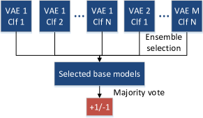
Figure 1: The ensemble selection approach. There are $M$ different VAE network candidate structures and $N$ different combinations of classifier hyper-parameter values.

3 Data and Results

3.1 Dataset

We conducted experiments using a dataset collected in the HumBug project . The HumBug project aims to detect malaria-vectoring mosquitoes through environment sound. The dataset used here includes 57 audio recordings with a total length of around 50 minutes. 736 seconds of these recordings contain sound of the Culex quinquefasciatus mosquitoes. We split these recordings into short audio clips, or what we call samples, with a duration of 0.1 seconds. Labels are given to each of these short audio clips. We resample to obtain a balanced dataset. Hence the dataset contains $7360$ positive samples (with mosquito sound) and $7360$ negative samples (no mosquito sound). A random sampling approach Li et al., 2017b , which randomly samples audio clips without replacement in the data set, was used to form the trainings set with $10\%$ of total samples. The remaining $90\%$ samples are used for testing.

3.2 Parameter values

Our target false positive rate threshold is set to $0.1$, i.e. we would like to minimise the missed detection while maintaining the false alarm rate to be below $10\%$. The SVM with the RBF kernel and the MFCC feature serves as the benchmark algorithm, as it leads to the best performance among a dozen of audio features (spectrogram, specentropy, etc.) and traditional classifiers (random forest, naive Bayes, etc.).

Candidate parameter values used to form the model library include the $2\nu$-SVM parameters: $\gamma:2^{-5},2^{-3},\ldots,2^{5}$ and $\nu_{+}/\nu_{-}:10^{-5},3\times 10^{-5},10^{-4},3\times 10^{-4},0.001,0.003,0.01,0.03,0.1,$ $0.2,0.3,0.4,\ldots,1$. The MFCC feature is 13-dimensional. To reduce feature dimension while maintaining most of detection power, we would like to use the VAE for feature re-representation. The candidate dimensions of the latent variable of the VAE include $3$ and $5$, while the number of nodes in the hidden layer can be either $10$ or $50$. Note that these choices are representative only and can vary for different datasets.

We initialise parameters of the VAE using a normal distribution with a standard deviation $0.01$. Adam Kingma and Ba, (2014) is used in the optimisation of the VAE. The cost-sensitive detector forms an ensemble of 100 base models to produce the final prediction.

3.3 Results

We performed 100 simulation trials, in which each trial differs due to the random seed initialisation, hence producing different data partitions and initial parameter values. We see from Figure 2(b) and Figure 2(c) that the cost-sensitive SVM (CSSVM) framework is able to maintain the false positive rate below $0.1$ in all simulation trials. The SVM with the MFCC feature has impressive performance (Figure 2(a)), but it fails to control the false positive rate to be below our target value.

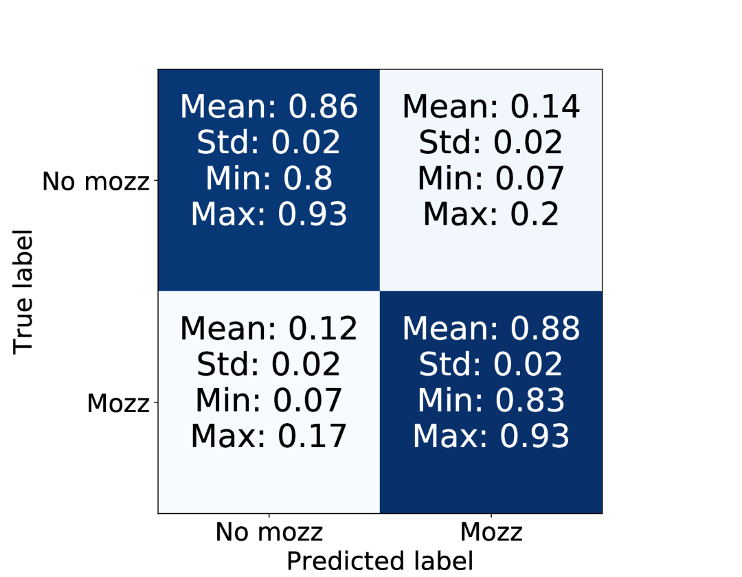
(a) MFCC, SVM

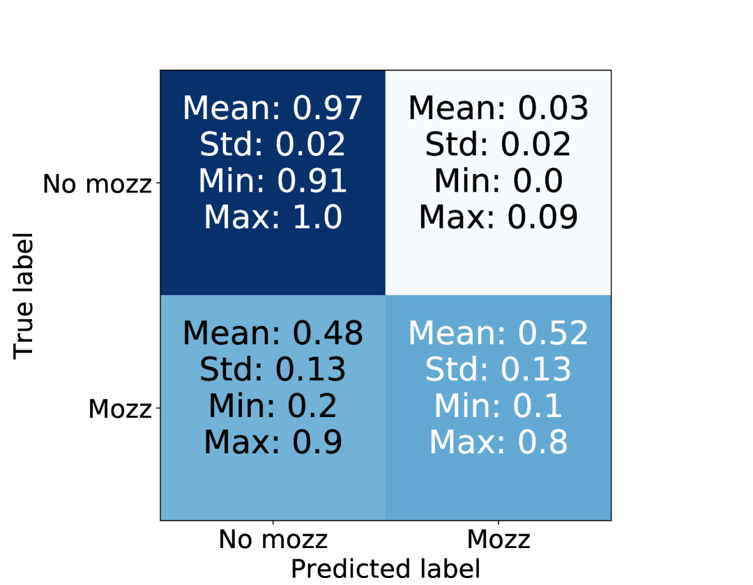
(b) MFCC, CSSVM

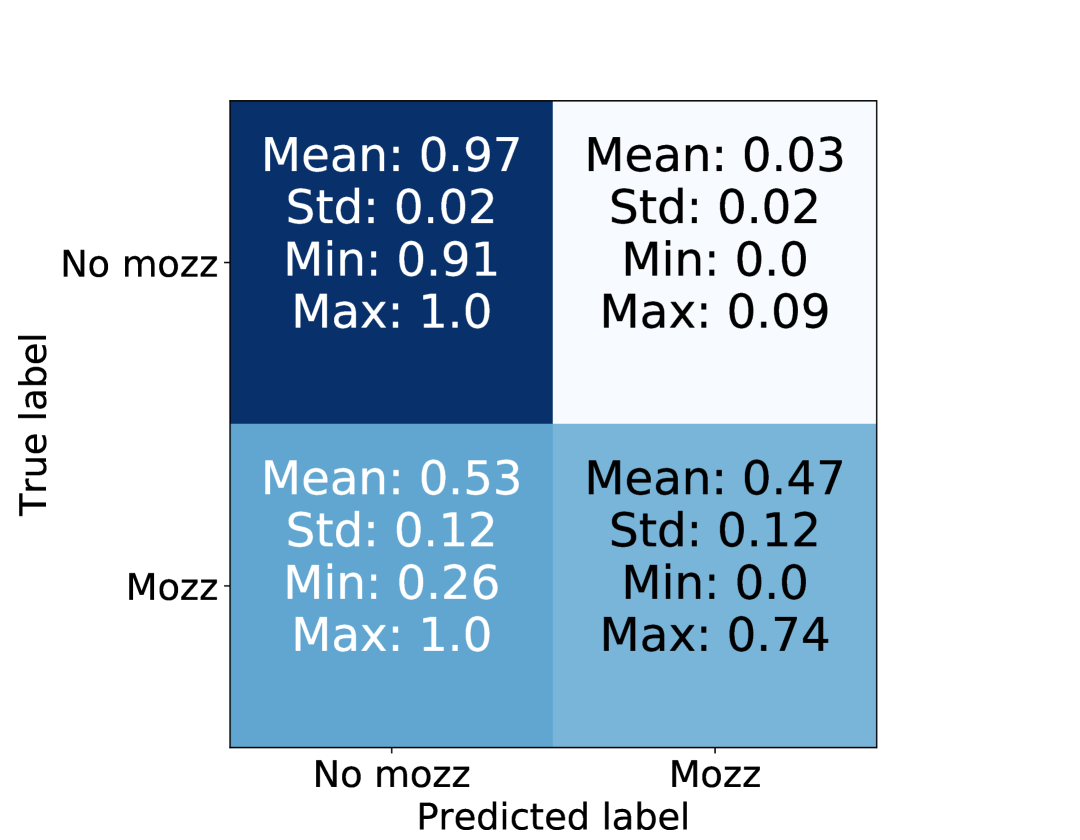
(c) MFCC+VAE, CSSVM

Figure 2: Confusion matrices of the test errors with different features and classifiers. “Mozz” is the positive class.

Although the VAE leads to slightly smaller sensitivity in detection performance for this dataset, the VAE provides a flexible mechanism to reduce feature dimension in the ensemble model. The reduction in the model size can be attractive in porting the model into embedded devices for environmental acoustic sensing Li et al., 2017b .

4 Conclusion

This paper presents a cost-sensitive classification framework for environmental audio sensing. The ensemble selection techniques are able to choose hyper-parameters of the feature extraction methods and the classifier in a principled manner. The proposed cost-sensitive SVM framework with the MFCC features is shown to ensure that the false positive rate lies below a pre-specified target value while minimising the false negative rate, by selecting a committee of best-performing individual models in a model library containing thousands of base models. We also consider VAE feature re-representations, which are helpful in selecting simple feature representations for low-power embedded systems.

Acknowledgements

This work is part-funded by a Google Impact Challenge award.

References

- Barchiesi et al., (2015) Barchiesi, D., Giannoulis, D., Stowell, D., and Plumbley, M. D. (2015). Acoustic scene classification: Classifying environments from the sounds they produce. IEEE Signal Processing Mag., 32(3):16–34.
- Blaauw and Bonada, (2016) Blaauw, M. and Bonada, J. (2016). Modeling and transforming speech using variational autoencoders. In Proc. Interspeech, pages 1770–1774.
- Caruana et al., (2006) Caruana, R., Munson, A., and Niculescu-Mizil, A. (2006). Getting the most out of ensemble selection. In Proc. Int. Conf. Data Mining (ICDM), pages 828–833.
- Chew et al., (2001) Chew, H.-G., Bogner, R. E., and Lim, C.-C. (2001). Dual -support vector machine with error rate and training size biasing. In Proc. Int. Conf. Acoustics, Speech and Signal Proc. (ICASSP), pages 1269–1272, Salt Lake City, USA.
- Cortes and Vapnik, (1995) Cortes, C. and Vapnik, V. (1995). Support-vector networks. Mach. Learn., 20(3):273–297.
- Davenport et al., (2010) Davenport, M. A., Baraniuk, R. G., and Scott, C. D. (2010). Tuning support vector machines for minimax and Neyman-Pearson classification. IEEE Trans. Pattern Anal. Mach. Intell., 32(10):1888–1898.
- Eronen et al., (2006) Eronen, A. J., Peltonen, V. T., Tuomi, J. T., Klapuri, A. P., Fagerlund, S., Sorsa, T., Lorho, G., and Huopaniemi, J. (2006). Audio-based context recognition. IEEE/ACM Trans. Speech Audio Process., 14:321–329.
- Hinton et al., (2012) Hinton, G., Deng, L., Yu, D., Dahl, G. E., r. Mohamed, A., Jaitly, N., Senior, A., Vanhoucke, V., Nguyen, P., Sainath, T. N., and Kingsbury, B. (2012). Deep neural networks for acoustic modeling in speech recognition: The shared views of four research groups. IEEE Signal Processing Mag., 29(6):82–97.
- Kelly et al., (2014) Kelly, B., Hollosi, D., Cousin, P., Leal, S., Iglár, B., and Cavallaro, A. (2014). Application of acoustic sensing technology for improving building energy efficiency. Procedia Computer Science, 32:661 – 664.
- Kingma and Ba, (2014) Kingma, D. and Ba, J. (2014). Adam: A method for stochastic optimization. arXiv:1412.6980.
- Kingma and Welling, (2014) Kingma, D. and Welling, M. (2014). Auto-encoding variational Bayes. In Proc. Intl. Conf. Learning Representations (ICLR).
- Lane et al., (2015) Lane, N. D., Georgiev, P., and Qendro, L. (2015). Deepear: Robust smartphone audio sensing in unconstrained acoustic environments using deep learning. In Proc. ACM Intl. J. Conf. Pervasive Ubiquitous Computing (UbiComp), pages 283–294.
- (13) Li, Y., Porter, E., Santorelli, A., Popović, M., and Coates, M. (2017a). Microwave breast cancer detection via cost-sensitive ensemble classifiers: Phantom and patient investigation. Biomed. Signal Process. Control, 31:366 – 376.
- (14) Li, Y., Zilli, D., Chan, H., Kiskin, I., Sinka, M., Roberts, S., and Willis, K. (2017b). Mosquito detection with low-cost smartphones: data acquisition for malaria research. In NIPS Workshop on Machine Learning for the Developing World, Long Beach, USA. arXiv:1711.06346.
- Lloret et al., (2015) Lloret, J., Canovas, A., Sendra, S., and Parra, L. (2015). A smart communication architecture for ambient assisted living. IEEE Commun. Mag., 53:26–33.
- Portelo et al., (2009) Portelo, J., Bugalho, M., Trancoso, I., Neto, J., Abad, A., and Serralheiro, A. (2009). Non-speech audio event detection. In Proc. Intl. Conf. Acoustics, Speech and Signal Proc. (ICASSP), pages 1973–1976.
- Salamon and Bello, (2017) Salamon, J. and Bello, J. P. (2017). Deep convolutional neural networks and data augmentation for environmental sound classification. IEEE Signal Process. Lett., 24(3):279–283.
- Schölkopf et al., (2000) Schölkopf, B., Smola, A. J., Williamson, R. C., and Bartlett, P. L. (2000). New support vector algorithms. Neural Comput., 12(5):1207–1245.
- Scholler and Purwins, (2011) Scholler, S. and Purwins, H. (2011). Sparse approximations for drum sound classification. IEEE J. Sel. Topics Signal Process., 5(5):933–940.
- Scott, (2007) Scott, C. (2007). Performance measures for neyman-pearson classification. IEEE Trans. Inf. Theory, 53:2852–2863.
- Sigtia et al., (2016) Sigtia, S., Stark, A. M., Krstulović, S., and Plumbley, M. D. (2016). Automatic environmental sound recognition: Performance versus computational cost. IEEE/ACM Trans. Speech Audio Process., 24:2096–2107.
- Tan and Sim, (2016) Tan, S. and Sim, K. C. (2016). Learning utterance-level normalisation using variational autoencoders for robust automatic speech recognition. In Proc. IEEE Spoken Language Technology Workshop (SLT), pages 43–49.
- Theunis et al., (2017) Theunis, J., Stevens, M., and Botteldooren, D. (2017). Sensing the environment. In Participatory Sensing, Opinions and Collective Awareness, pages 21–46. Springer International Publishing, Switzerland.
- Zilli et al., (2014) Zilli, D., Parson, O., Merrett, G. V., and Rogers, A. (2014). A hidden Markov model-based acoustic cicada detector for crowdsourced smartphone biodiversity monitoring. J. Artif. Intell. Res., 51:805–827.