Collective modes of an imbalanced unitary Fermi gas

Abstract

We study theoretically the collective mode spectrum of a strongly imbalanced two-component unitary Fermi gas in a cigar-shaped trap, where the minority species forms a gas of polarons. We describe the collective breathing mode of the gas in terms of the Fermi liquid kinetic equation taking collisions into account using the method of moments. Our results for the frequency and damping of the longitudinal in-phase breathing mode are in good quantitative agreement with an experiment by Nascimbène et al. [Phys. Rev. Lett. 103, 170402 (2009)] and interpolate between a hydrodynamic and a collisionless regime as the polarization is increased. A separate out-of phase breathing mode, which for a collisionless gas is sensitive to the effective mass of the polaron, however, is strongly damped at finite temperature, whereas the experiment observes a well-defined oscillation.

I Introduction

Landau’s Fermi liquid theory accounts for the fact that many normal state Fermi systems behave in a qualitatively similar way to a noninteracting Fermi gas Landau (1957a, b, 1959). The central assumption of the theory is the adiabatic continuity of excitations, meaning that excitations of the interacting system are characterized by the same quantum numbers of spin $\sigma=\uparrow,\downarrow$ and momentum ${\bf p}$ as the noninteracting system Pines and Nozières (1994); Lifshitz and Pitaevskii (2006); Giuliani and Vignale (2005). The robustness of this picture relies on phase space arguments and does not depend on the strength of the interparticle interaction.

Over the past ten years, the two-spin-component Fermi quantum gas has emerged as a new Fermi liquid Lobo et al. (2006). For small polarization $P=(N_{\uparrow}-N_{\downarrow})/(N_{\uparrow}+N_{\downarrow})$ ($N_{\uparrow,\downarrow}$ being the total number of atoms of each species), the ground state is a superfluid Zwerger (2016). As the polarization is increased beyond the Clogston-Chandrasekar limit, there is a first order phase transition to a Fermi liquid where both species coexist Chevy and Salomon (2012); Recati and Stringari (2012). In particular, the extreme limit $P\to 1$ describes a single spin-$\downarrow$ quasiparticle interacting with a majority spin-$\uparrow$ Fermi sea (a “polaron”) characterized by an effective mass $m^{*}$, energy $E_{p}=-\alpha E_{F}$ (where $E_{F}$ is the Fermi energy of the majority species), and quasiparticle residue. These parameters have been studied extensively at zero temperature Chevy (2006); Combescot et al. (2007); Veillette et al. (2008); Combescot and Giraud (2008); Prokof’ev and Svistunov (2008a, b); Punk et al. (2009); Vlietinck et al. (2013); Goulko et al. (2016).

There are three ways to measure the polaron parameters. First, through the equation of state Navon et al. (2010). Second, by measuring the radiofrequency spectrum, which has a pronounced quasiparticle peak at the polaron energy with a weight proportional to the quasiparticle residue Schirotzek et al. (2009); Kohstall et al. (2012); Scazza et al. (2017). The third method – which we are interested in here – measures the effective mass dynamically by exciting collective mode oscillations Nascimbène et al. (2009).

The experiment Nascimbène et al. (2009) by Nascimbène et al. studied the collective breathing modes in the longitudinal direction of an elongated harmonic trap as a function of polarization. At low polarization, both spin components oscillate in phase due to the strong coupling between them. At larger polarization, an additional out-of-phase mode was observed. In the $P\to 1$ limit its frequency was identified with the collisionless value $2\omega^{*}_{z}$, where $\omega^{*}_{z}$ is the axial trap frequency renormalized by the interaction of the minority atoms with the majority background Lobo et al. (2006):

$$\omega^{*}_{z} =\omega_{z}\sqrt{\frac{m}{m^{*}}(1+\alpha)}.$$ (1)

Reference Nascimbène et al. (2009) obtained the polaron effective mass from Eq. (1) after linearly extrapolating the experimental out-of-phase breathing mode frequency to $P=1$. This has resulted in a value at unitarity of $m^{*}/m=1.17(10)$, in close agreement with theoretical results Combescot and Giraud (2008); Combescot et al. (2009); Pilati and Giorgini (2008); Prokof’ev and Svistunov (2008a, b); Vlietinck et al. (2013).

In a subsequent theory paper Recati and Stringari (2010), Recati and Stringari analyzed the out-of-phase collective mode using a scaling ansatz with mean-field interactions but without collisions, and obtained a frequency behaviour that disagreed with the experiment Nascimbène et al. (2009) at lower values of polarization. However, at these polarizations collisions can become important so that a full theoretical description of the experiment is still lacking.

In this paper, we analyze the collective breathing mode spectrum of a Fermi liquid taking into account finite-temperature effects, mean-field interactions and also quasiparticle collisions. The theoretical framework that allows us to do this is the Landau-Boltzmann equation, which we solve using the method of moments. This method has already been successfully applied to study the collective modes of balanced Fermi gases Riedl et al. (2008); Chiacchiera et al. (2009); Lepers et al. (2010); Chiacchiera et al. (2011); Pantel et al. (2012); Chiacchiera et al. (2013). The paper is structured as follows: in Sec. II, we solve the quasiparticle kinetic equation for a trapped and strongly imbalanced Fermi gas using the single-polaron parameters obtained in Combescot and Giraud (2008). We obtain the eigenmodes in a trap by expanding the distribution function in small deviations from equilibrium in a finite-dimensional basis of trial functions. In this way, both the single-particle contribution to the kinetic equation as well as the collision integral can be reduced to a set of linear equations whose eigenvalues determine the collective mode frequencies. We present results for collective modes for the experimental setup of Ref. Nascimbène et al. (2009), and compare with the experimental results.

II Collective modes

In the high-polarization limit of the imbalanced Fermi gas, the minority atoms (spin-$\downarrow$) form a dilute gas of polarons that interact with the majority species (spin-$\uparrow$). Within Fermi liquid theory, the quasi-classical evolution of the minority and majority distribution function $n_{\sigma}({\bf r},{\bf p},t)$ is described by the coupled Landau-Boltzmann kinetic equation [setting $\hbar=1$],

$$\biggl{[}\partial_{t}+\frac{\partial\varepsilon_{\sigma}({\bf r},{\bf p})}{\partial{\bf p}}\cdot\frac{\partial}{\partial{\bf r}}-\frac{\partial\varepsilon_{\sigma}({\bf r},{\bf p})}{\partial{\bf r}}\cdot\frac{\partial}{\partial{\bf p}}\biggr{]}n_{\sigma}({\bf r},{\bf p})$$

$$\quad=-I_{\sigma}[n_{\uparrow},n_{\downarrow}],$$ (2)

where the distribution functions of each spin state are normalized as

$$N_{\sigma} =\int d^{3}r\,n_{\sigma}({\bf r})\quad{\rm with}\quad n_{\sigma}({\bf r})=\int\frac{d^{3}p}{(2\pi)^{3}}n_{\sigma}({\bf r},{\bf p}).$$ (3)

$\varepsilon_{\sigma}({\bf r},{\bf p})$ is the energy of a quasiparticle with spin $\sigma$ and momentum ${\bf p}$ at position ${\bf r}$:

$$\varepsilon_{\sigma}({\bf r},{\bf p}) =\frac{p^{2}}{2m_{\sigma}}+U_{\sigma}({\bf r})+V({\bf r}).$$ (4)

We take $m_{\downarrow}=m^{*}$, the effective polaron mass, and $m_{\uparrow}=m$, the bare atom mass. The spin-independent harmonic trapping potential with trapping frequencies $\omega_{i}$ ($i=x,y,z$) is given by

$$V({\bf r})=\sum_{i=x,y,z}\frac{m\omega_{i}^{2}}{2}r_{i}^{2}.$$ (5)

$U_{\sigma}=U_{\sigma}[n_{\uparrow}(\mathbf{r}),n_{\downarrow}(\mathbf{r})]$ are the mean-field interactions experienced by each spin component, which are deduced from the single-polaron parameters at zero temperature. For the minority species, the mean field potential is given by the single-polaron energy $U_{\downarrow}=-\alpha E_{F}(\mathbf{r})$, while the majority mean field $U_{\uparrow}$ is chosen such that the total force acting on the system vanishes,

$$U_{\downarrow}[n_{\uparrow},n_{\downarrow}] =-\alpha\frac{(6\pi^{2})^{2/3}}{2m}n_{\uparrow}^{2/3}({\bf r})$$ (6)

$$U_{\uparrow}[n_{\uparrow},n_{\downarrow}] =-\frac{2}{3}\alpha\frac{(6\pi^{2})^{2/3}}{2m}\frac{n_{\downarrow}({\bf r})}{n_{\uparrow}^{1/3}({\bf r})}.$$ (7)

The distribution in thermal equilibrium is the Fermi-Dirac distribution with chemical potential $\mu_{\sigma}$ Lifshitz and Pitaevskii (2006); Pines and Nozières (1994)

$$n_{\sigma}^{\rm eq}({\bf r},{\bf p}) =\frac{1}{e^{\beta(\varepsilon_{\sigma}({\bf r},{\bf p})-\mu_{\sigma})}+1}.$$ (8)

Unlike for a noninteracting gas, Eq. (8) is a complicated self-consistent expression since $n_{\sigma}^{\rm eq}({\bf r},{\bf p})$ enters $\varepsilon_{\sigma}({\bf r},{\bf p})$ through the mean-field potential. The attractive mean-field potential increases the particle density in the trap center.

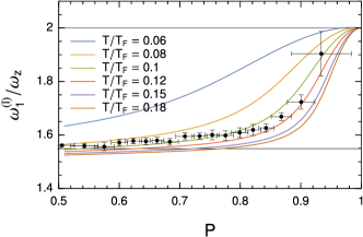
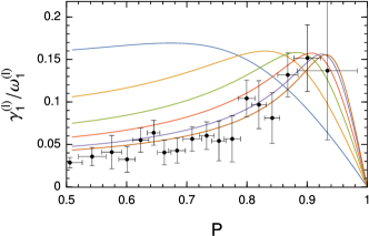
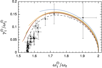
Figure 1: (a) Frequency and (b) damping of the longitudinal breathing mode of an imbalanced Fermi gas in an anisotropic trap with aspect ratio $\lambda=0.075$ as a function of polarization for different temperatures $T/T_{F}=0.06,0.08,0.1,0.12,0.15$ and $0.18$, respectively. The thin black lines in the first figure denote the collisionless limit $\omega_{\rm cl}=2\omega_{z}$ and the hydrodynamic limit $\omega_{\rm hd}=\sqrt{12/5}\omega_{z}$. (c) Scaling plot of frequency versus damping, which indicates the presence of a single dominant scattering lifetime. The black dashed line is the parametric estimate of Eq. (25). The experimental data points are taken from Ref. Nascimbène et al. (2009).

Interactions change the distribution function through the collision integral

$$I_{\sigma}[n_{\uparrow},n_{\downarrow}]=\int\frac{d^{3}p_{1}}{(2\pi)^{3}}\,\int d\Omega\,\frac{d\sigma}{d\Omega}\,|{\bf v}_{\rm rel}|\, \biggl{[}n_{\sigma}({\bf r},{\bf p},t)\,n_{\bar{\sigma}}({\bf r},{\bf p}_{1},t)\,(1-n_{\sigma}({\bf r},{\bf p}^{\prime},t))\,(1-n_{\bar{\sigma}}({\bf r},{\bf p}_{1}^{\prime},t))$$

$$\qquad-n_{\sigma}({\bf r},{\bf p}^{\prime},t)\,n_{\bar{\sigma}}({\bf r},{\bf p}_{1}^{\prime},t)\,(1-n_{\sigma}({\bf r},{\bf p},t))\,(1-n_{\bar{\sigma}}({\bf r},{\bf p}_{1},t))\biggr{]},$$ (9)

where $\bar{\sigma}$ denotes the opposite spin species of $\sigma$, ${\bf v}_{\rm rel}$ the relative velocity of colliding particles, and $\frac{d\sigma}{d\Omega}=\bigl{(}\frac{m_{\rm red}}{2\pi}f_{\uparrow\downarrow}\bigr{)}^{2}$ the differential scattering cross section, where the scattering amplitude $f_{\uparrow\downarrow}$ is linked to the single-polaron energy by $f_{\uparrow\downarrow}=\frac{\partial E_{p}}{\partial n_{\uparrow}}$. The first line of the collision integral describes the depopulation of the state $({\bf p},\sigma)$ by collisions with a quasiparticle $({\bf p}_{1},\bar{\sigma})$ to a final state $({\bf p}^{\prime},\sigma)$ and $({\bf p}_{1}^{\prime},\bar{\sigma})$. The second line describes the reverse process $({\bf p}^{\prime},\sigma)+({\bf p}_{1}^{\prime},\bar{\sigma})\to({\bf p},\sigma)+({\bf p}_{1},\bar{\sigma})$. The collisions are constrained by energy and momentum conservation. Writing in the center-of-mass frame ${\bf p}=\frac{m_{\sigma}}{M}{\bf P}+{\bf q}$ and ${\bf p}_{1}=\frac{m_{\bar{\sigma}}}{M}{\bf P}-{\bf q}$, where $M=m+m^{*}$ is the total mass and ${\bf P}={\bf p}+{\bf p}_{1}$ the total momentum, we have ${\bf p}^{\prime}=\frac{m_{\sigma}}{M}{\bf P}+{\bf q}^{\prime}$ and ${\bf p}_{1}^{\prime}=\frac{m_{\bar{\sigma}}}{M}{\bf P}-{\bf q}^{\prime}$, where $|{\bf q}|=|{\bf q}^{\prime}|$, as well as ${\bf v}_{\rm rel}={\bf q}/m_{\rm red}$ with $m_{\rm red}=\frac{mm^{*}}{m+m^{*}}$ the reduced mass. The integration over the angle element $d\Omega$ in Eq. (9) describes the change in the solid angle between ${\bf q}$ and ${\bf q}^{\prime}$.

Solving the full collision integral is a complicated task. Here, we use an approximate method to study small oscillations around the equilibrium distribution (see, e.g., Refs. Chiacchiera et al. (2009); Pantel et al. (2012) for more details). To this end, we expand the distribution function as

$$n_{\sigma}({\bf r},{\bf p},t)=n^{\rm eq}_{\sigma}({\bf r},{\bf p})$$

$$\qquad+n^{\rm eq}_{\sigma}({\bf r},{\bf p})(1-n^{\rm eq}_{\sigma}({\bf r},{\bf p}))\Phi_{\sigma}({\bf r},{\bf p},t),$$ (10)

where $n^{\rm eq}_{\sigma}({\bf r},{\bf p})$ is the equilibrium distribution (8). The prefactor in Eq. (10) is chosen such that $\Phi_{\sigma}$ can be interpreted as a potential perturbation that corrects the quasiparticle energy $\varepsilon_{\sigma}$. The collision integral then reads:

$$I_{\sigma}[\Phi_{\sigma},\Phi_{\bar{\sigma}}]=\int\frac{d^{3}p_{1}}{(2\pi)^{3}}\,\int d\Omega\,\frac{d\sigma}{d\Omega}\,|{\bf v}_{\rm rel}|$$

$$\times n^{\rm eq}_{\sigma}({\bf r},{\bf p})\,n^{\rm eq}_{\bar{\sigma}}({\bf r},{\bf p}_{1})\,(1-n^{\rm eq}_{\sigma}({\bf r},{\bf p}^{\prime}))\,(1-n^{\rm eq}_{\bar{\sigma}}({\bf r},{\bf p}_{1}^{\prime}))$$

$$\times\left[\Phi_{\sigma}({\bf r},{\bf p},t)+\Phi_{\bar{\sigma}}({\bf r},{\bf p}_{1},t)-\Phi_{\sigma}({\bf r},{\bf p}^{\prime},t)-\Phi_{\bar{\sigma}}({\bf r},{\bf p}_{1}^{\prime},t)\right].$$ (11)

This complicated kinetic equation can be solved approximately by expanding the perturbation $\Phi_{\sigma}({\bf r},{\bf p})$ in a suitably chosen set of basis functions

$$\Phi_{\sigma}({\bf r},{\bf p},t)=e^{-i\omega t}\sum_{j}c_{j,\sigma}\psi_{j,\sigma}({\bf r},{\bf p}),$$ (12)

where we assume a harmonic time-dependence with frequency $\omega$. Substituting this form in Eq. (2), multiplying by $\psi_{i}({\bf r},{\bf p})$, and integrating over ${\bf r}$ and ${\bf p}$ reduces the kinetic equation to a set of linear equations of the form

$$\omega M_{1}+M_{2}+M_{3}+C =0,$$ (13)

where $M_{1},M_{2},$ and $C$ are matrices with coefficients

$$(M_{1})^{\sigma\sigma^{\prime}}_{ij} =-i\int\frac{d^{3}rd^{3}p}{(2\pi)^{3}}\,\psi_{i,\sigma}({\bf r},{\bf p})\,n^{\rm eq}_{\sigma^{\prime}}({\bf r},{\bf p})$$

$$\quad\times(1-n^{\rm eq}_{\sigma^{\prime}}({\bf r},{\bf p}))\psi_{j,\sigma^{\prime}}({\bf r},{\bf p})$$ (14)

$$(M_{2})^{\sigma\sigma^{\prime}}_{ij} =\int\frac{d^{3}rd^{3}p}{(2\pi)^{3}}\,\psi_{i,\sigma}({\bf r},{\bf p})\,\Bigl{[}(\nabla_{\bf p}\varepsilon_{\sigma}({\bf r},{\bf p}))\cdot\nabla_{\bf r}$$

$$\quad-(\nabla_{\bf r}\varepsilon_{\sigma}({\bf r},{\bf p}))\cdot\nabla_{\bf p}\bigr{]}n^{\rm eq}_{\sigma^{\prime}}({\bf r},{\bf p})$$

$$\quad\times(1-n^{\rm eq}_{\sigma^{\prime}}({\bf r},{\bf p}))\psi_{j,\sigma^{\prime}}({\bf r},{\bf p})$$ (15)

$$(M_{3})^{\sigma\sigma^{\prime}}_{ij} =-\int\frac{d^{3}rd^{3}p}{(2\pi)^{3}}\,\psi_{i,\sigma}({\bf r},{\bf p})\,(\nabla_{\bf p}n^{\rm eq}_{\sigma}({\bf r},{\bf p}))\cdot$$

$$\quad\times\biggl{[}\nabla_{\bf r}\frac{\partial U_{eq,\sigma}}{\partial n^{\rm eq}_{\sigma^{\prime}}({\bf r})}\delta n_{j,\sigma^{\prime}}({\bf r})\biggr{]}$$ (16)

$$(C)^{\sigma\sigma^{\prime}}_{ij} =\int\frac{d^{3}rd^{3}p}{(2\pi)^{3}}\,\psi_{i,\sigma}({\bf r},{\bf p})\,I_{\sigma}[\psi_{j,\sigma^{\prime}}({\bf r},{\bf p}),0],$$ (17)

where

$$\delta n_{j,\sigma^{\prime}}({\bf r}) =\int\frac{d^{3}p}{(2\pi)^{3}}n^{\rm eq}_{\sigma^{\prime}}({\bf r},{\bf p})(1-n^{\rm eq}_{\sigma^{\prime}}({\bf r},{\bf p}))\psi_{j,\sigma^{\prime}}({\bf r},{\bf p}).$$ (18)

The eigenmodes $\omega$ are obtained by computing the matrices $M_{1},M_{2},M_{3},$ and $C$ numerically and solving the eigenvalue problem for the matrix $-M_{1}^{-1}[M_{2}+M_{3}+C]$. For the breathing mode oscillation, a suitable set of basis functions is

$$\psi_{1,\sigma} =x^{2}+y^{2}$$ (19)

$$\psi_{2,\sigma} =z^{2}$$ (20)

$$\psi_{3,\sigma} =xp_{x}+yp_{y}$$ (21)

$$\psi_{4,\sigma} =zp_{z}$$ (22)

$$\psi_{5,\sigma} =p_{x}^{2}+p_{y}^{2}$$ (23)

$$\psi_{6,\sigma} =p_{z}^{2}.$$ (24)

The computation of the moments is intricate, and we relegate the details of this calculation and the results to App. A.

II.1 In-phase mode

We first discuss the lowest-frequency breathing mode. For a weakly imbalanced Fermi gas, this mode corresponds to an in-phase breathing mode of both spin species, which changes at large polarization, where it describes the breathing mode of the majority species. In the following, we choose the same parameters as in the experiment Nascimbène et al. (2009): the aspect ratio of the trap is $\lambda=\omega_{z}/\omega_{r}=0.075$ and we explore the unitary limit $a\to\infty$ at low temperatures. The temperature scale is set by the majority density as $T_{F}=\omega_{0}(6N_{\uparrow})^{1/3}$ with $\omega_{0}=(\omega_{z}\omega_{r}^{2})^{1/3}$, which corresponds to the Fermi energy of a noninteracting trapped single-component gas.

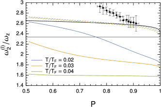
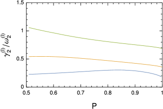
Figure 2: (a) Frequency and (b) damping of the longitudinal out-of-phase breathing mode of an imbalanced Fermi gas in an anisotropic trap with aspect ratio $\lambda=0.075$ as a function of polarization for three different temperatures $T/T_{F}=0.02,0.03$ and $0.04$. For comparison, we show the collisionless results as dashed lines. The continuous black line indicates the zero temperature scaling result of Ref. Recati and Stringari (2012) and the thin black line denotes the collisionless limit Eq. (1). The experimental data points are taken from Ref. Nascimbène et al. (2009).

Figure 1 shows the in-phase breathing mode as a function of polarization for several temperatures $T/T_{F}=0.06,0.08,0.1,0.12,0.15$, and $0.18$. Figure 1(a) shows the collective mode frequency, which clearly displays a crossover between a hydrodynamic and a collisionless limit. The oscillation frequency in the collisionless limit $P\to 1$ is equal to twice the trap frequency, $\omega_{\rm cl}=2\omega_{z}$. In the hydrodynamic limit $P\ll 1$, the frequency can be estimated by taking moments of the $z^{2}$ dynamic structure factor yielding $\omega_{\rm hd}=\sqrt{12/5}\omega_{z}$ Nascimbène et al. (2009). Both limiting cases are indicated by thin black lines. The solution of the Fermi liquid kinetic theory is in good agreement with the experimental measurements and provides an accurate description of the collisionless-to-hydrodynamic crossover with the experimental parameters. At unitarity, the Clogston-Chandrasekar limit is at $P=0.75$, which puts a lower limit on the applicability of our theory. Nevertheless, even below that, in the superfluid phase, there is only a small quantitative discrepancy with the experiment. Figure 1(b) shows the damping of the collective mode frequency. Again, our theoretical calculations are in good quantitative agreement with the experiment Nascimbène et al. (2009), with optimal agreement at a temperature $T\approx 0.12T_{F}$, the same optimal temperature as for the collective mode frequency.

Finally, in Fig. 1(c), we show a reduced plot of damping versus frequency, which does not contain the polarization. All results approximately collapse onto a single scaling curve. This indicates the presence of a single dominant relaxation time $\tau$ and is consistent with a thermodynamic argument for the crossover, which predicts that frequency and damping satisfy *[][; §78.]landau66

$$\omega^{2}=\omega_{\rm cl}^{2}+\frac{\omega_{\rm hd}^{2}-\omega_{\rm cl}^{2}}{1+i\omega\tau},$$ (25)

where $\omega$ is a complex number, the real part of which sets the mode frequency $\omega_{1}$ and the imaginary part sets the damping $\gamma_{1}$. This scaling solution is shown as a black dashed line in Fig. 1(c) for comparison.

In addition to the longitudinal in-phase breathing mode, there is also a radial in-phase oscillation. Because the radial trapping frequency is much larger than the longitudinal frequency, $\omega_{r}\gg\omega_{z}$, collisions are much less efficient here (as can be seen, for example, from Eq. (25)). For all temperatures in our calculation, the oscillation is only very weakly damped and remains close to the collisionless value $\omega_{1}^{(r)}=2\omega_{r}$ for all polarizations. We do not plot this mode.

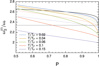
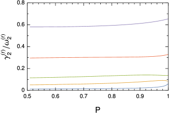
Figure 3: (a) Frequency and (b) damping of the radial out-of-phase breathing mode of an imbalanced Fermi gas in an anisotropic trap with aspect ratio $\lambda=0.075$ as a function of polarization for different temperatures $T/T_{F}=0.02,0.04,0.06,0.1$ and $0.15$. For comparison, we show the collisionless results as dashed lines. The continuous black line indicates the zero temperature scaling result of Ref. Recati and Stringari (2012) and the thin black line denotes the collisionless limit Eq. (1).

II.2 Out-of-phase mode

There is a second higher-frequency breathing mode excitation for each trap direction, which corresponds to an out-of-phase breathing mode at small polarization and reduces to an oscillation of the minority atoms at large polarization. This limit is of particular interest as the collisionless oscillation frequency, Eq. (1), depends on the polaron mass.

Figure 2 shows our results for the frequency and damping of the longitudinal out-of-phase for three different temperatures $T/T_{F}=0.02,0.03$, and $0.04$. Different from the in-phase oscillation, the collisionless limit cannot be reached by changing the polarization, and we find that the mode is very strongly damped at any polarization. Indeed, for any larger temperatures $T/T_{F}>0.05$, the mode is completely overdamped. For comparision, we include the collisionless frequencies as dashed lines in Fig. 2(a). We find that at small temperature and high polarization, the difference of the breathing mode from the single polaron frequency [Eq. (1)] is proportional to the radius of the minority cloud, which depends on the polarization as

$$\frac{R_{\downarrow}}{R_{\uparrow}}\sim\left(\frac{1-P}{1+P}\right)^{1/6}.$$ (26)

This result was previously established by Recati and Stringari Recati and Stringari (2010), who analyzed the mode at zero temperature neglecting collisions by combining a scaling ansatz and a density functional for the ground state energy of the imbalanced gas. We show their result in Fig. 2 for comparison (black line). At finite temperature, this effect is less pronounced and decreases with increasing temperature, and our calculation suggests a linear dependence of the collisionless breathing mode frequency on the polarization for $P<0.9$.

The calculated frequencies are at odds with the experimental measurements Nascimbène et al. (2009) (black points in Fig. 2). While already the collisionless results differs from the experimental data, it was suggested in Recati and Stringari (2010) that collisions could be responsible for this discrepancy. Our calculations, which do include collisions, would seem to refute this claim. We find that the damping of this mode is very significant, to the extent that it would be overdamped for all values of $P$ at the experimental temperatures, rendering it difficult to observe, in contradiction with the experiment.

The radial out-of-phase breathing mode persists over a larger range of temperatures since collisions are less efficient compared to the longitudinal oscillation. Figure 3 shows the frequency and damping of this mode for temperatures $T/T_{F}=0.02,0.04,0.06,0.1$, and $0.15$. Collisions decrease the oscillation frequency compared to the collisionless case (dashed lines) with a strong damping at any polarization. The oscillation reduces to the collisionless frequency only at small temperatures.

III Summary and Conclusions

In conclusion, we have studied the collective breathing modes of a strongly imbalanced unitary Fermi gas, assuming that it can be described as an interacting gas of minority polarons and majority atoms. We have solved the kinetic equation in an elongated harmonic trap taking into account quasiparticle collisions. For the in-phase breathing mode, our results provide an accurate description of both frequency and damping observed in the experiment by Nascimbène et al. Nascimbène et al. (2009). The theory displays a crossover between a collisionless limit at large polarization, where the mode frequency $\omega$ is much larger than the inverse collision time $1/\tau$, $\omega\tau\gg 1$, and a hydrodynamic limit $\omega\tau\ll 1$, where single excitations decay rapidly. Our theory appears to be reliable down to the critical polarization $P\sim 0.7$, below which a superfluid core forms at the trap center. By contrast, our results for the out-of-phase breathing mode oscillation differ from the findings in Nascimbène et al. (2009). While our results are consistent with predictions from a scaling ansatz for the collisionless gas Recati and Stringari (2012), taking into account collisions does not resolve the discrepancy between theory and experiment.

Appendix A Method of moments

We determine the lowest breathing mode excitations of a spin-imbalanced Fermi gas by solving the linearized Boltzmann equation using the method of moments. This appendix describes the details of the calculation.

We define the potential energy per spin species:

$$E_{\rm pot,\sigma} =\int d^{3}r\,V_{\rm trap}\,n^{\rm eq}_{\sigma}$$ (27)

and the kinetic energy

$$E_{\rm kin,\sigma} =\int\frac{d^{3}rd^{3}p}{(2\pi)^{3}}\,\frac{p^{2}}{2m_{\sigma}}\,n^{\rm eq}_{\sigma}.$$ (28)

They are related through the virial theorem

$$\frac{E_{{\rm kin},\sigma}}{E_{{\rm pot},\sigma}} =1-\tilde{\chi}_{\sigma},$$ (29)

where $\chi_{\sigma}$ is defined as

$$\tilde{\chi}_{\sigma} =-\frac{1}{2E_{\rm pot,\sigma}}\int d^{3}\tilde{r}\,n^{\rm eq}_{\sigma}\tilde{r}\,\frac{\partial U_{\sigma}^{\rm eq}}{\partial\tilde{r}}.$$ (30)

The eigenmodes are determined by solving the equation

$$\det(A+B) =0.$$ (31)

$A$ is the matrix of moments of the streaming term, and $B$ the matrix for the collision integral. They are:

$$A^{\sigma\sigma} =\left(\begin{matrix}\dfrac{2i\omega\omega_{0}(1+\varphi_{\sigma})}{\omega_{r}^{2}}&\dfrac{i\omega\omega_{0}(1+\varphi_{\sigma})}{2\omega_{r}^{2}}&1&0&\dfrac{i\omega}{\omega_{0}}\dfrac{m_{\sigma}}{m}&\dfrac{i\omega}{2\omega_{0}}\dfrac{m_{\sigma}}{m}\\[4.30554pt] \dfrac{2i\omega\omega_{0}(1+\varphi_{\sigma})}{\omega_{r}^{2}}&\dfrac{3i\omega\omega_{0}(1+\varphi_{\sigma})}{\omega_{r}^{2}}&0&2&2\dfrac{i\omega}{\omega_{0}}\dfrac{m_{\sigma}}{m}&\dfrac{i\omega}{\omega_{0}}\dfrac{m_{\sigma}}{m}\\[4.30554pt] 2(1+2\varphi_{1,\sigma\sigma}-\varphi_{3,\sigma\sigma})&\varphi_{1,\sigma\sigma}-\varphi_{3,\sigma\sigma}&-\dfrac{i\omega}{\omega_{0}}\dfrac{m_{\sigma}}{m}&0&-2\dfrac{\omega_{r}^{2}}{\omega_{0}^{2}}\dfrac{m_{\sigma}}{m}\left(1-\tilde{\chi}_{\sigma}-\chi_{\sigma\sigma}+2\chi_{\sigma\sigma}^{\prime}\right)&\dfrac{\omega_{r}^{2}}{\omega_{0}^{2}}\dfrac{m_{\bar{\sigma}}}{m}\left(\chi_{\sigma\sigma}-2\chi_{\sigma\sigma}^{\prime}\right)\\[4.30554pt] 2(\varphi_{1,\sigma\sigma}-\varphi_{3,\sigma\sigma})&2+3\varphi_{1,\sigma\sigma}-\varphi_{3,\sigma\sigma}&0&-\dfrac{i\omega}{\omega_{0}\lambda^{2}}\dfrac{m_{\sigma}}{m}&2\dfrac{\omega_{r}^{2}}{\omega_{0}^{2}}\dfrac{m_{\sigma}}{m}\left(\chi_{\sigma\sigma}-2\chi_{\sigma\sigma}^{\prime}\right)&-2\dfrac{\omega_{r}^{2}}{\omega_{0}^{2}}\dfrac{m_{\sigma}}{m}\left(1-\tilde{\chi}_{\sigma}-\chi_{\sigma\sigma}+2\chi_{\sigma\sigma}^{\prime}\right)\\[4.30554pt] \dfrac{im\omega\omega_{0}}{m_{\sigma}\omega_{r}^{2}(1-\tilde{\chi}_{\sigma})}&\dfrac{im\omega\omega_{0}}{2m_{\sigma}\omega_{r}^{2}(1-\tilde{\chi}_{\sigma})}&-\dfrac{m}{m_{\sigma}}&0&2\dfrac{i\omega}{\omega_{0}}&\dfrac{i\omega}{2\omega_{0}}\\[4.30554pt] \dfrac{im\omega\omega_{0}}{m_{\sigma}\omega_{r}^{2}(1-\tilde{\chi}_{\sigma})}&\dfrac{im\omega\omega_{0}}{2m_{\sigma}\omega_{r}^{2}(1-\tilde{\chi}_{\sigma})}&0&-\dfrac{m}{m_{\sigma}}&\dfrac{i\omega}{\omega_{0}}&\dfrac{3}{2}\dfrac{i\omega}{\omega_{0}}\end{matrix}\right),$$ (32)

$$A^{\sigma\bar{\sigma}} =\left(\begin{matrix}0&0&0&0&0&0\\[4.30554pt] 0&0&0&0&0&0\\[4.30554pt] 2(2\varphi_{1,\sigma\bar{\sigma}}-\varphi_{3,\sigma\bar{\sigma}})&\varphi_{1,\sigma\bar{\sigma}}-\varphi_{3,\sigma\bar{\sigma}}&0&0&2\dfrac{\omega_{r}^{2}}{\omega_{0}^{2}}\dfrac{m_{\bar{\sigma}}}{m}(\chi_{\sigma\bar{\sigma}}-2\chi_{\sigma\bar{\sigma}}^{\prime})&\dfrac{\omega_{r}^{2}}{\omega_{0}^{2}}\dfrac{m_{\bar{\sigma}}}{m}(\chi_{\sigma\bar{\sigma}}-2\chi_{\sigma\bar{\sigma}}^{\prime})\\[4.30554pt] 2(\varphi_{1,\sigma\bar{\sigma}}-\varphi_{3,\sigma\bar{\sigma}})&3\varphi_{1,\sigma\bar{\sigma}}-\varphi_{3,\sigma\bar{\sigma}}&0&0&2\dfrac{\omega_{r}^{2}}{\omega_{0}^{2}}\dfrac{m_{\bar{\sigma}}}{m}(\chi_{\sigma\bar{\sigma}}-2\chi_{\sigma\bar{\sigma}}^{\prime})&\dfrac{\omega_{r}^{2}}{\omega_{0}^{2}}\dfrac{m_{\bar{\sigma}}}{m}(\chi_{\sigma\bar{\sigma}}-2\chi_{\sigma\bar{\sigma}}^{\prime})\\[4.30554pt] 0&0&0&0&0&0\\[4.30554pt] 0&0&0&0&0&0\end{matrix}\right),$$ (33)

$$B^{\sigma\tau} =\begin{pmatrix}0&0&0&0&0&0\\ 0&0&0&0&0&0\\ 0&0&\dfrac{\pm 1}{\tau_{A\sigma}}&0&0&0\\ 0&0&0&\dfrac{\pm 1}{\lambda^{2}\tau_{A\sigma}}&0&0\\ 0&0&0&0&\dfrac{-1}{\tau_{B\sigma}}-\dfrac{m_{\sigma}\pm m_{\tau}}{M}\dfrac{1}{\tau_{C\sigma}}\mp\dfrac{m_{\sigma}m_{\tau}}{M^{2}}\left(\dfrac{1}{\tau_{D\sigma}}+\dfrac{1}{\tau_{E\sigma}}\right)&\dfrac{1}{\tau_{B\sigma}}+\dfrac{m_{\sigma}\pm m_{\tau}}{M}\dfrac{1}{\tau_{C\sigma}}\pm\dfrac{m_{\sigma}m_{\tau}}{M^{2}}\left(\dfrac{1}{\tau_{D\sigma}}-\dfrac{1}{\tau_{E\sigma}}\right)\\[4.30554pt] 0&0&0&0&\dfrac{2}{\tau_{B\sigma}}+\dfrac{m_{\sigma}\pm m_{\tau}}{M}\dfrac{2}{\tau_{C\sigma}}\pm\dfrac{2m_{\sigma}m_{\tau}}{M^{2}}\left(\dfrac{1}{\tau_{D\sigma}}-\dfrac{1}{\tau_{E\sigma}}\right)&-\dfrac{2}{\tau_{B\sigma}}-\dfrac{m_{\sigma}\pm m_{\tau}}{M}\dfrac{2}{\tau_{C\sigma}}\mp\dfrac{m_{\sigma}m_{\tau}}{M^{2}}\dfrac{2}{\tau_{D\sigma}}\end{pmatrix},$$ (34)

where the upper sign for $B$ applies if $\sigma=\tau$ and the lower if $\sigma\neq\tau$ and we define the dimensionless quantities (use rescaled coordinates $\tilde{r}_{i}=\omega_{i}r_{i}/\omega_{0}$):

$$\chi_{\sigma\tau} =-\frac{1}{2E_{\rm pot,\sigma}}\int d^{3}\tilde{r}\,n^{\rm eq}_{\tau}\,\tilde{r}\,\frac{\partial U_{\sigma}^{\rm eq}}{\partial n^{\rm eq}_{\tau}}\,\frac{\partial n^{\rm eq}_{\sigma}}{\partial\tilde{r}}$$ (35)

$$\chi_{\sigma\tau}^{\prime} =\frac{3}{4E_{\rm pot,\sigma}}\int d^{3}\tilde{r}\,n^{\rm eq}_{\sigma}\,n^{\rm eq}_{\tau}\,\frac{\partial U_{\sigma}^{\rm eq}}{\partial n^{\rm eq}_{\tau}}$$ (36)

$$\varphi_{\sigma} =\frac{1}{10E_{\rm pot,\sigma}}\int d^{3}\tilde{r}\,\tilde{r}^{2}\frac{\partial n^{\rm eq}_{\sigma}}{\partial\tilde{r}}\,\frac{\partial U_{\sigma}^{\rm eq}}{\partial\tilde{r}}\,\frac{1}{1+\dfrac{1}{m\omega_{0}^{2}\tilde{r}}\dfrac{\partial U_{\sigma}^{\rm eq}}{\partial\tilde{r}}}$$ (37)

$$\varphi_{1,\sigma\tau} =\frac{1}{10E_{\rm pot,\sigma}}\int d^{3}\tilde{r}\,\tilde{r}^{2}\frac{\partial n^{\rm eq}_{\sigma}}{\partial\tilde{r}}\,\frac{\partial n^{\rm eq}_{\tau}}{\partial\tilde{r}}\,\frac{\partial U_{\sigma}^{\rm eq}}{\partial n^{\rm eq}_{\tau}}\,\frac{1}{1+\dfrac{1}{m\omega_{0}^{2}\tilde{r}}\dfrac{\partial U_{\tau}^{\rm eq}}{\partial\tilde{r}}}$$ (38)

$$\varphi_{3,\sigma\tau} =-\frac{1}{2E_{\rm pot,\sigma}}\int d^{3}\tilde{r}\,\tilde{r}n^{\rm eq}_{\sigma}\,\frac{\partial n^{\rm eq}_{\tau}}{\partial\tilde{r}}\,\frac{\partial U_{\sigma}^{\rm eq}}{\partial n^{\rm eq}_{\tau}}\,\frac{1}{1+\dfrac{1}{m\omega_{0}^{2}\tilde{r}}\dfrac{\partial U_{\tau}^{\rm eq}}{\partial\tilde{r}}}.$$ (39)

The various relaxation times can be calculated along the lines of Ref. Vichi (2000):

$$\frac{1}{\tau_{i\sigma}} =\int_{0}^{\infty}d\tilde{r}\,\tilde{r}^{2}\,\int_{0}^{\infty}dP\,P^{2}\,\int_{0}^{\infty}dq\,q^{5}\,\frac{d\sigma}{d\Omega}\,\int_{-1}^{1}d(x,y)\,n_{\downarrow}({\bf r},{\bf p})\,n_{\uparrow}({\bf r},{\bf p}_{1})\,(1-n_{\downarrow}({\bf r},{\bf p}^{\prime}))\,(1-n_{\uparrow}({\bf r},{\bf p}_{1}^{\prime}))\times g_{i,\sigma}(x,y),$$ (40)

where $g_{A,\sigma}(x,y)=\frac{\beta\omega_{0}\tilde{r}^{2}(1-xy)}{6\pi^{2}m_{\rm red}E_{{\rm pot},\sigma}}$ and

$$g_{i,\sigma}(x,y) =\frac{\beta}{\pi^{2}m_{\rm red}m_{\sigma}^{2}\omega_{0}E_{{\rm kin},\sigma}}\begin{cases}\dfrac{q^{2}}{40}(1+x^{2}+y^{2}-3x^{2}y^{2})&i=B\\[8.61108pt] \dfrac{qP}{30}(x+y)(1-xy)&i=C\\[8.61108pt] \dfrac{P^{2}}{10}(1+x^{2}+y^{2}-3xy)&i=D\\[8.61108pt] \dfrac{P^{2}}{4}(x-y)^{2}&i=E\end{cases}.$$ (41)

References

• Landau (1957a) L. D. Landau, “Theory of the Fermi Liquid,” Sov. Phys. JETP 3, 920 (1957a).
• Landau (1957b) L. D. Landau, “Oscillations in a Fermi Liquid,” Sov. Phys. JETP 5, 101 (1957b).
• Landau (1959) L. D. Landau, “On the Theory of the Fermi Liquid,” Sov. Phys. JETP 35, 70 (1959).
• Pines and Nozières (1994) D. Pines and P. Nozières, Theory Of Quantum Liquids, Volume I: Normal Fermi Liquids (Westview Press, 1994).
• Lifshitz and Pitaevskii (2006) E. M. Lifshitz and L. P. Pitaevskii, Course of Theoretical Physics, Vol. 9: Statistical Physics, Part 2 (Butterworth-Heinemann, 2006).
• Giuliani and Vignale (2005) G. Giuliani and G. Vignale, Quantum Theory of the Electron Liquid (Cambridge University Press, 2005).
• Lobo et al. (2006) C. Lobo, A. Recati, S. Giorgini,  and S. Stringari, “Normal State of a Polarized Fermi Gas at Unitarity,” Phys. Rev. Lett. 97, 200403 (2006).
• Zwerger (2016) W. Zwerger, “Strongly Interacting Fermi Gases,” in Proceedings of the International School of Physics “Enrico Fermi” - Course 191 “Quantum Matter at Ultralow Temperatures”, edited by M. Inguscio, W. Ketterle, S. Stringari,  and G. Roati (IOS Press, Amsterdam; SIF Bologna, 2016).
• Chevy and Salomon (2012) F. Chevy and C. Salomon, “Thermodynamics of Fermi Gases,” in The BCS–BEC Crossover and the Unitary Fermi Gas, edited by W. Zwerger (Springer, 2012) Chap. 11.
• Recati and Stringari (2012) A. Recati and S. Stringari, “Normal Phase of Polarised Strongly Interacting Fermi Gases,” in The BCS–BEC Crossover and the Unitary Fermi Gas, edited by W. Zwerger (Springer, 2012) Chap. 12.
• Chevy (2006) F. Chevy, “Universal Phase Diagram of a Strongly Interacting Fermi Gas with Unbalanced Spin Populations,” Phys. Rev. A 74, 063628 (2006).
• Combescot et al. (2007) R. Combescot, A. Recati, C. Lobo,  and F. Chevy, “Normal State of Highly Polarized Fermi Gases: Simple Many-Body Approaches,” Phys. Rev. Lett. 98, 180402 (2007).
• Veillette et al. (2008) M. Veillette, E. G. Moon, A. Lamacraft, L. Radzihovsky, S. Sachdev,  and D. E. Sheehy, “Radio-Frequency Spectroscopy of a Strongly Imbalanced Feshbach-Resonant Fermi Gas,” Phys. Rev. A 78, 033614 (2008).
• Combescot and Giraud (2008) R. Combescot and S. Giraud, “Normal State of Highly Polarized Fermi Gases: Full Many-Body Treatment,” Phys. Rev. Lett. 101, 050404 (2008).
• Prokof’ev and Svistunov (2008a) N. Prokof’ev and B. Svistunov, “Fermi-Polaron Problem: Diagrammatic Monte Carlo Method for Divergent Sign-Alternating Series,” Phys. Rev. B 77, 020408 (2008a).
• Prokof’ev and Svistunov (2008b) N. V. Prokof’ev and B. V. Svistunov, “Bold Diagrammatic Monte Carlo: A Generic Sign-Problem Tolerant Technique for Polaron Models and Possibly Interacting Many-Body Problems,” Phys. Rev. B 77, 125101 (2008b).
• Punk et al. (2009) M. Punk, P. T. Dumitrescu,  and W. Zwerger, “Polaron-to-Molecule Transition in a Strongly Imbalanced Fermi Gas,” Phys. Rev. A 80, 053605 (2009).
• Vlietinck et al. (2013) J. Vlietinck, J. Ryckebusch,  and K. Van Houcke, “Quasiparticle Properties of an Impurity in a Fermi Gas,” Phys. Rev. B 87, 115133 (2013).
• Goulko et al. (2016) O. Goulko, A. S. Mishchenko, N. Prokof’ev,  and B. Svistunov, “Dark Continuum in the Spectral Function of the Resonant Fermi Polaron,” Phys. Rev. A 94, 051605 (2016).
• Navon et al. (2010) N. Navon, S. Nascimbène, F. Chevy,  and C. Salomon, “The Equation of State of a Low-Temperature Fermi Gas with Tunable Interactions,” Science 328, 729–732 (2010).
• Schirotzek et al. (2009) A. Schirotzek, C.-H. Wu, A. Sommer,  and M. W. Zwierlein, “Observation of Fermi Polarons in a Tunable Fermi Liquid of Ultracold Atoms,” Phys. Rev. Lett. 102, 230402 (2009).
• Kohstall et al. (2012) C. Kohstall, M. Zaccanti, M. Jag, A. Trenkwalder, P. Massignan, G. M. Bruun, F. Schreck,  and R. Grimm, “Metastability and Coherence of Repulsive Polarons in a Strongly Interacting Fermi Mixture,” Nature 485, 615 (2012).
• Scazza et al. (2017) F. Scazza, G. Valtolina, P. Massignan, A. Recati, A. Amico, A. Burchianti, C. Fort, M. Inguscio, M. Zaccanti,  and G. Roati, “Repulsive Fermi Polarons in a Resonant Mixture of Ultracold ${}^{6}\mathrm{Li}$ Atoms,” Phys. Rev. Lett. 118, 083602 (2017).
• Nascimbène et al. (2009) S. Nascimbène, N. Navon, K. J. Jiang, L. Tarruell, M. Teichmann, J. McKeever, F. Chevy,  and C. Salomon, “Collective Oscillations of an Imbalanced Fermi Gas: Axial Compression Modes and Polaron Effective Mass,” Phys. Rev. Lett. 103, 170402 (2009).
• Combescot et al. (2009) R. Combescot, S. Giraud,  and X. Leyronas, “Analytical Theory of the Dressed Bound State in Highly Polarized Fermi Gases,” EPL 88, 60007 (2009).
• Pilati and Giorgini (2008) S. Pilati and S. Giorgini, “Phase Separation in a Polarized Fermi Gas at Zero Temperature,” Phys. Rev. Lett. 100, 030401 (2008).
• Recati and Stringari (2010) A. Recati and S. Stringari, “Spin Oscillations of the Normal Polarized Fermi Gas at Unitarity,” Phys. Rev. A 82, 013635 (2010).
• Riedl et al. (2008) S. Riedl, E. R. Sánchez Guajardo, C. Kohstall, A. Altmeyer, M. J. Wright, J. Hecker Denschlag, R. Grimm, G. M. Bruun,  and H. Smith, “Collective Oscillations of a Fermi Gas in the Unitarity Limit: Temperature Effects and the Role of Pair Correlations,” Phys. Rev. A 78, 053609 (2008).
• Chiacchiera et al. (2009) S. Chiacchiera, T. Lepers, D. Davesne,  and M. Urban, “Collective Modes of Trapped Fermi Gases With In-Medium Interaction,” Phys. Rev. A 79, 033613 (2009).
• Lepers et al. (2010) T. Lepers, D. Davesne, S. Chiacchiera,  and M. Urban, “Numerical Solution of the Boltzmann Equation for the Collective Modes of Trapped Fermi Gases,” Phys. Rev. A 82, 023609 (2010).
• Chiacchiera et al. (2011) S. Chiacchiera, T. Lepers, D. Davesne,  and M. Urban, “Role of Fourth-Order Phase-Space Moments in Collective Modes of Trapped Fermi Gases,” Phys. Rev. A 84, 043634 (2011).
• Pantel et al. (2012) P.-A. Pantel, D. Davesne, S. Chiacchiera,  and M. Urban, “Trap Anharmonicity and Sloshing Mode of a Fermi Gas,” Phys. Rev. A 86, 023635 (2012).
• Chiacchiera et al. (2013) S. Chiacchiera, S. Davesne, T. Enss,  and M. Urban, “Damping of the Quadrupole Mode in a Two-Dimensional Fermi Gas,” Phys. Rev. A 88, 053616 (2013).
• Landau and Lifshitz (1966) L. D. Landau and E. M. Lifshitz, Course of Theoretical Physics, Vol. 6: Fluid Mechanics (Butterworth-Heinemann, 1966).
• Vichi (2000) L. Vichi, “Collisional Damping of the Collective Oscillations of a Trapped Fermi Gas,” J. Low T. Phys. 121, 177 (2000).