Cumulant analysis of the statistical properties of a deterministically thermostated harmonic oscillator

Abstract

Usual approach to investigate the statistical properties of deterministically thermostated systems is to analyze the regime of the system motion. In this work the cumulant analysis is used to study the properties of the stationary probability distribution function of the deterministically thermostated harmonic oscillators. This approach shifts attention from the investigation of the geometrical properties of solutions of the systems to the studying a probabilistic measure. The cumulant apparatus is suitable for studying the correlations of dynamical variables, which allows one to reveal the deviation of the actual probabilistic distribution function from canonical one and to evaluate it. Three different thermostats, namely the Nosé-Hoover, Patra-Bhatacharya and Hoover-Holian ones, were investigated. It is shown that their actual distribution functions are non-canonical because of nonlinear coupling of the oscillators with thermostats. The problem of ergodicity of the deterministically thermostated systems is discussed.

I Introduction

The molecular dynamics approach is widely used to investigate equilibrium thermodynamic properties of many body systems. The thermostats, that is physical equations of motion modified by a dynamic temperature control tool, are commonly used to simulate systems of particles at constant temperature. There are stochastic and deterministic thermostats.

In the case of a stochastic thermostat the thermodynamic ensemble is described by a set of stochastic Langevin equations of motion. This approach allow us to create a canonical ensemble. But in some cases this approach is unsuitable because of very slow converging to the equilibrium state.

Deterministic thermostats are an alternative way to solve the problem. In this case the ensemble is described by a set of deterministic nonlinear ordinary differential equations in an extended phase space. Additional phase variables are one, two or more pseudo-friction coefficients which obey specific equations of motion. These equations are arranged in such a way that they can control some macroscopic parameters of the ensemble. Thus, Nosé nose and Nosé-Hoover (NH) hoover thermostats enhance the phase space by one variable and control the kinetic temperature. More complicated thermostats by Patra-Bhattacharya (PB) patra and Hoover-Holian (HH) hh add two variables and control two parameters of the ensemble. As a result of generalization of these methods in kus ; mart ; wat ; patra2 , families of thermostats for which the above are special cases were proposed. Samoletov and Vasiev samolet propose a dynamic principle underlying a range of thetmostats derived using fundamental laws of statistical physics. Their approach covers both stochastic and deterministic schemes.

The statistical properties of the stationary dynamical system are described by the stationary probability distribution function (PDF) the domain of definition of which is the whole phase space. Such PDF obeys the stationary Liouville continuity equation corresponding to the system under consideration. For the stationary dynamical system coupled with any deterministic thermostat one of the solution of the equation is the PDF which is canonical in the physical phase space and is Gaussian with respect to the additional phase variables. But the actual PDF obtained by solving the equations of motion can be different and it is, of course, not canonical.

The ergodicity of the system is another problem. The system is ergodic if its probabilistic measure is invariant or, in other words, its PDF doesn’t depend on initial conditions. In the case of thermostated systems the usual approach to this problem is to analyze the regime of the system motion. It boils down to the study of the character of the filling of the phase space with the trajectories of the system.

In the quasi-periodic regime of motion the system evidently is not ergodic because in this case there exist invariant tori separating the system phase space into invariant domains depending on the initial conditions. The chaotic regime is much more consistent with the concept of ergodicity.

The statistical properties of the deterministically thermostated systems are investigated mainly on the base of the model of a one-dimensional harmonic oscillator. The authors of the articles hoover ; posch ; legoll showed that under some conditions in the system of the harmonic oscillator coupled with the Nosé and NH thermostats there exist invariant tori. The conditions are determined by the system parameters and the initial conditions.

A detailed study of the ergodicity of the singly and doubly thermostated harmonic oscillators in the chaotic regime gave inconclusive results. The harmonic oscillators coupled with the Nosé and NH thermostats were shown posch ; hoover to be nonergodic. Patra and Bhattacharya patra3 , when working with the harmonic oscillator coupled with the two-chain NH thermostat, find that it does not generate the canonical distribution and does not provide ergodicity of the system. In other papers hoover2 ; hoover3 ; patra4 ; hoover4 ; hoover5 the conclusion was drawn that this thermostat is ergodic and the ergodicity of some other thermostats is being discussed.

An undeniable evidence of the nonergodicity of a dynamical system can be the existence of a conserved integral of motion. Such integrals are known for the harmonic oscillators thermostated by NH, HH, NH chain and some other thermostats samolet ; samolet2 . But, in general, the problem of the ergodicity of the deterministically thermostated harmonic oscillator is still open.

In this work, the statistical properties of the harmonic oscillator coupled with the NH, PB and HH thermostats are studied by means of the cumulant approach. This method is a powerful tool for studying the correlation properties of nonlinear dynamical systems. Its use, together with the numerical approach makes it possible to investigate the canonicity and ergodicity of the created thermodynamic ensembles. The minimal information on the cumulant approach, which is necessary to understand the matter under discussion, is given in Sec. II. The statistical properties of the NH system are considered in Sec. III. In Sec. IV, the properties of the PB and HH thermostats are discussed. In the final section, the conclusive considerations are given. In the Application, one can find some intermediate equations that are mentioned in the text.

II Degenerated equations for cumulants.

The purpose of this work is a statistical analysis of deterministic dynamic systems, the evolution of which is determined by the equations of motion. of the form

$$\dot{\textbf{q}}=\textbf{g}(\textbf{q}),$$ (1)

where q is a vector of phase variables and g is a vector nonlinear differentiable function. The distribution of the system in the phase space is described by a PDF $W(\textbf{q},t)$. The existence of the stationary limit $W(\textbf{q})=W(\textbf{q},t\rightarrow\infty)$ of this function is assumed.

The characteristic function $\theta(\textbf{v},t)$ which is a Fourier transform of the $W(\textbf{q},t)$

$$\theta(\textbf{v},t)=\int e^{\imath(\textbf{qv})}W(\textbf{q},t)d\textbf{q}$$ (2)

is an equivalent way to describe the distribution of the system. Moments and cumulants are coefficients of expansion in a series of the characteristic function and its logarithm respectively

$$\theta(\textbf{v},t) = \sum_{m_{1},...m_{n}=0}^{\infty}\frac{\alpha(t)_{m_{1},...m_{n}}^{q_{1},...q_{n}}}{m_{1}!...m_{n}!}(\imath v_{1})^{m_{1}}...(\imath v_{n})^{m_{n}}$$ (3)

$$= \exp\left[\sum_{m_{1},...m_{n}=0}^{\infty}\frac{\kappa(t)_{m_{1},...m_{n}}^{q_{1},...q_{n}}}{m_{1}!...m_{n}!}(\imath v_{1})^{m_{1}}...(\imath v_{n})^{m_{n}}\right].$$

Here $\alpha(t)_{m_{1},...m_{n}}^{q_{1},...q_{n}}$ is the joint moment and $\kappa(t)_{m_{1},...m_{n}}^{q_{1},...q_{n}}$ is the the joint cumulant of $n$ variables $q_{1},...q_{n}$ and $\imath$ is the imaginary unit. The full set of moments or cumulants completely represents $W(\textbf{q},t)$ as long as the series (3) converge at all $\{v_{i}\}_{i=1}^{n}$.

But the role of the moments and cumulants in the analysis of statistical, in particular correlation, properties of a dynamical system is very different. If the joint moment of some dynamical variables is different from zero, it does not mean the existence of a statistical dependence of these variables yet. But the difference from zero of the joint cumulant uniquely manifest such a dependence.

Hereinafter, the concept of cumulant brackets going to be required. They are the angle brackets with arguments separated by commas. If arguments are single variables the cumulant bracket coincides with the corresponding cumulant, for example $\langle q_{i},q_{j},q_{i}\rangle=\kappa_{2,1}^{q_{i},q_{j}}$. In the case if one or several arguments are functions the operation ”to open cumulant brackets” is need in order to represent a cumulant bracket as a function of cumulants malakh ; primak .

The cumulant analysis is widely used for statistical analysis of stochastic differential equations in the theory of Markov processes malakh ; primak . To analyze deterministic differential equations this approach was applied by V. Kontorovich kant . In this work the set of degenerated equations for cumulants was obtained as the limit of the full set, in which the amplitudes of random forces tend to zero.

Here we propose simplified derivation of the degenerate equations for cumulants assuming, that all necessary conditions are satisfied. The PDF $W(\textbf{q},t)$ corresponding to the system (1) obeys the Liouville continuity equation

$$\frac{\partial W}{\partial t}+\frac{\partial\left(\textbf{K}_{1}W\right)}{\partial\textbf{q}}=\frac{\partial W}{\partial t}+\frac{\partial\left(\dot{\textbf{q}}W\right)}{\partial\textbf{q}}=0.$$ (4)

The notation $\textbf{K}_{1}=\textbf{g}(\textbf{q})$ for kinetic coefficients is introduced to bring our notations in line with the established those in the existing literature malakh ; primak ; kant . Let $f(\textbf{q})$ be a phase variables function. Then

$$\frac{d}{dt}\left\langle f(\textbf{q})\right\rangle = \int f(\textbf{q})\frac{\partial W}{\partial t}d\textbf{q}=$$ (5)

$$= -\int f(\textbf{q})\frac{\partial(\textbf{K}_{1}W)}{\partial\textbf{q}}d\textbf{q}=\left\langle\textbf{K}_{1}\frac{\partial f(\textbf{q})}{\partial\textbf{q}}\right\rangle,$$

where the angle brackets mean the statistical average. In the third term, the Liouville equation (4) was used to replace the time derivative and the last one is obtained as the result of the integration by parts.

Substituting monomials of the variables $q_{i}$ insread of $f(\textbf{q})$ we arrive at the set of equations for the moments

$$\frac{d}{dt}\left\langle q_{i}\right\rangle = \left\langle K_{1i}\right\rangle,$$

$$\frac{d}{dt}\left\langle q_{i}q_{j}\right\rangle = \left\langle q_{i}K_{1j}\right\rangle+\left\langle K_{1i}q_{j}\right\rangle=2\left\{\left\langle q_{i}K_{1j}\right\rangle\right\}_{s},$$

$$\frac{d}{dt}\left\langle q_{i}q_{j}q_{k}\right\rangle = \left\langle q_{i}q_{j}K_{1k}\right\rangle+\left\langle K_{1i}q_{j}q_{k}\right\rangle+\left\langle q_{i}K_{1j}q_{k}\right\rangle=$$

$$= 3\left\{\left\langle q_{i}q_{j}K_{1k}\right\rangle\right\}_{s},$$

$$\vdots$$

Here the symbol $n\{\ldots\}_{s}$ is the Stratonovich brackets. It denotes the completely symmetrical sum of the variables which are enclosed in the brackets. The number before the brackets is the number of terms in the expression.

To obtain the equations for cumulants one should use the interrelationship of cumulants and moments. As a result, the equations get the same form as for moments if the moment brackets (statistical averaging) are replaced by the cumulant ones malakh ; primak .

$$\frac{d}{dt}\left\langle q_{i}\right\rangle = \left\langle K_{1i}\right\rangle,$$

$$\frac{d}{dt}\left\langle q_{i},q_{j}\right\rangle = 2\left\{\left\langle q_{i},K_{1j}\right\rangle\right\}_{s},$$ (7)

$$\frac{d}{dt}\left\langle q_{i},q_{j},q_{k}\right\rangle = 3\left\{\left\langle q_{i},q_{j},K_{1k}\right\rangle\right\}_{s},$$

$$\vdots$$

In the next sections the stationary statistical properties of the different thermostated systems are studied. In each case, only a limited number of stationary equations from the infinite set (II) are analyzed.

The phase space dimension of the systems under consideration is three or four. The phase variables are the coordinates $x$, the momenta $p$ and one or two friction coefficients $\zeta$ and $\xi$, $\textbf{q}=(x,p,\zeta(,\xi))$. For the sake of simplicity the upper indices in the cumulants are omitted but, instead, the order of the variables in subscripts are fixed, namely

$$\kappa_{k,l,m(,n)}^{x,p,\zeta(,\xi)}\equiv\kappa_{k,l,m(,n)}.$$ (8)

III Nosé-Hoover thermostat

III.1 Equations of motion and canonical PDF

Dynamics of a harmonic oscillator which is coupled with the NH thermostat obeys the set of three ordinary differential equations of the first order

$$\dot{x} = \frac{p}{m},$$

$$\dot{p} = -kx-\zeta p,$$ (9)

$$\dot{\zeta} = \frac{1}{\tau}\left(\frac{p^{2}}{mT}-1\right).$$

Here $\textbf{q}=(x,p,\zeta)$ is a vector of phase variables, $m$ and $\tau$ are the masses of the oscillator and the thermostat, $k$ is the coefficient of elasticity and $T$ is the temperature.

The well known feature of the system (9) is that the stationary PDF

$$W_{c}(\textbf{q})\propto\exp\left\{-\frac{p^{2}}{2mT}-\frac{kx^{2}}{2T}\right\}\exp\left\{-\frac{\zeta^{2}}{2\tau^{-1}}\right\}$$ (10)

obeys the stationary Liouville continuity equation $\frac{\partial}{\partial\textbf{q}}\left(\dot{\textbf{q}}W(\textbf{q})\right)=0$. The marginal PDF in the physical phase subspace $(x,p)$ is canonical and the whole PDF is Gaussian. This function is completely determined by three nonzero cumulants of the second order

$$\kappa_{2,0,0}=\frac{T}{k},\;\kappa_{0,2,0}=Tm,\;\kappa_{0,0,2}=\frac{1}{\tau}.$$ (11)

All other cumulants are equal to zero. The phase variables, distribution of which in a phase space are described by such a function, are statistically independent.

III.2 Equations for cumulants

The kinetic coefficients of the system are

$$\textbf{K}_{1}=\left(K_{1x},K_{1p},K_{1\zeta}\right)=\left(\frac{p}{m},-kx-\zeta p,\frac{1}{\tau}\left(\frac{p^{2}}{mT}-1\right)\right).$$ (12)

The equations for cumulants are an infinite set of nonlinear algebraic equations. In this section the stationary equations corresponding to nonstationary ones with time derivatives from $\dot{\kappa}_{1,0,0}$ to $\dot{\kappa}_{0,0,4}$ are analyzed. The number of the equations is 34. But the key equations are written out here only. To the left of each expression, the corresponding time derivative is written to specify from which equation for cumulants this stationary equation was obtained.

The first equation is

$$\dot{\kappa}_{1,0,0}:\;\;\left\langle K_{1x}\right\rangle=\left\langle\frac{p}{m}\right\rangle=\frac{1}{m}\kappa_{0,1,0}=0.$$ (13)

The solution gives a zero value of the cumulant $\kappa_{0,1,0}$. The second representative equation is more complicated

$$\dot{\kappa}_{0,0,1}:\;\;\left\langle K_{1\zeta}\right\rangle=\frac{1}{\tau}\left(\frac{\left\langle p^{2}\right\rangle}{mT}-1\right)=\frac{1}{\tau}\left(\frac{\kappa_{0,2,0}}{mT}-1\right)=0.$$ (14)

In the last term the dependence of the second moment on cumulants (37) and the equality to zero of the cumulant $\kappa_{0,1,0}$ (13) are taken into account. Thus, the equation (14) gives $\kappa_{0,2,0}=Tm$. The characteristic features of these solutions are that they are completely determined by the equations for cumulants and both of them coincide with the corresponding cumulants (11) of the canonical PDF (10).

There are a number of other zero solutions of the equations having the same features. They are all cumulants of the first order, the cumulants $\kappa_{1,1,0}$, $\kappa_{1,0,1}$ and $\kappa_{0,1,1}$ of the second order, all cumulants of the third order with the exception of $\kappa_{1,1,1}$, and eight cumulants of the fourth order.

The rest of the cumulants are the solutions of other type. They obey the set of equations

$$\dot{\kappa}_{1,1,0} : \;\;k\kappa_{2,0,0}+\kappa_{1,1,1}-T=0,$$

$$\dot{\kappa}_{2,0,1} : \;\;\frac{1}{\tau T}\kappa_{2,2,0}+2\kappa_{1,1,1}=0,$$

$$\dot{\kappa}_{0,2,1} : \;\;\frac{1}{\tau Tm}\kappa_{0,4,0}+\frac{2Tm}{\tau}-2k\kappa_{1,1,1}-2Tm\kappa_{0,0,2}=0$$

$$\dot{\kappa}_{3,1,0} : \;\;\frac{3}{m}\kappa_{2,2,0}-k\kappa_{4,0,0}=0,$$ (15)

$$\dot{\kappa}_{1,3,0} : \;\;\frac{1}{m}\kappa_{0,4,0}-3k\kappa_{2,2,0}-6Tm\kappa_{1,1,1}=0,$$

$$\dot{\kappa}_{1,1,2} : \;\;k\kappa_{2,0,2}+2\kappa_{1,1,1}\kappa_{0,0,2}-\frac{4}{\tau}\kappa_{1,1,1}=0$$

To obtain these equations the solutions for the canonical cumulants were taken into account. The set contains six equations for seven unknowns. So, the set is underdetermined and has an infinite number of solutions. To solve these equations one need to take one of the unknowns as a parameter. Let it be $\kappa_{1,1,1}$. Then

$$\kappa_{2,0,0} = \frac{T}{k}-\frac{1}{k}\kappa_{1,1,1},$$ (16)

$$\kappa_{0,0,2} = \frac{1}{\tau}+\frac{1}{T}\left(\frac{3}{\tau}-\frac{4k}{m}\right)\kappa_{1,1,1}.$$ (17)

These cumulants differ from canonical ones (11) because of the summands proportional to $\kappa_{1,1,1}$. The fourth order cumulants, entering into Eqs. (15), are directly proportional to $\kappa_{1,1,1}$. For example

$$\kappa_{0,4,0}=6Tm(m-k\tau)\kappa_{1,1,1}.$$ (18)

Nonzero value of the cumulant $\kappa_{1,1,1}$ means that the variables $x$, $p$ and $\zeta$ are statistically dependent. It is easy to understand from the structure of the equations for cumulants that the cumulant $\kappa_{1,1,1}$ in Eqs. (15) arises because of the nonlinear term $\zeta p$ in the equations of motion. This means that the coupling of the oscillator with the thermostat, which is provided by this term, leads to the appearance of non-physical correlations of the dynamic variables and, thus, to the non-canonicity of the ensemble.

So, the analysis of the equations for cumulants shows that all cumulants can be divided into two groups. The first one includes the cumulants which are unique solutions of the equations. They are $\kappa_{0,2,0}$ and all zero valued cumulants. These cumulants coincide with those of the canonical PDF and in what follows are referred to as canonical. The other group includes the cumulants which depend on a free parameter, similarly to the solutions of Eqs. (15). These cumulants are nonzero because of the statistical dependence of phase variables which is the cause of the distinction between the actual PDF and the canonical one. They below are termed as non-canonical.

Further analysis of the equations for cumulants gives no any new information. To achieve further progress in studying the system behavior the equations (9) were solved numerically.

III.3 Numerical approach

The purpose of the numerical approach is to calculate the cumulants of the stationary PDF as time averages along the trajectory of the system motion. But cumulants are not statistical averages. They are non-linear combinations of moments, which are statistical averages. The moments can be calculated as time averages asymptotically at $t_{av}\rightarrow\infty$ converging to their limiting values

$$\langle x^{k}p^{m}\zeta^{n}\rangle_{t}=\frac{1}{t_{av}}\int_{t}^{t+t_{av}}ds\>x(s)^{k}p(s)^{m}\zeta(s)^{n}.$$ (19)

Here $t_{av}$ is the time of averaging, $x(s)$, $p(s)$ and $\zeta(s)$ are the values of the phase variables on the system trajectory at time $s$. In order to calculate the cumulant as a time average, one need to express it in terms of time averaged moments malakh ; primak and calculate this combination. See for example Eqs. (42, 43).

The motion type of the system is determined by its parameters and initial conditions. The analysis of the system behavior was performed at fixed parameters $k=m=1$ and $T=0.5$. The thermostat mass was chosen $\tau=10$ in the regular regime and $\tau\leq 2$ in the chaotic one. The initial conditions are specified later when the results are discussed. To solve the equations (9) the modification hockney of the Verlet algorithm verlet is used with the time step $\triangle t=0.01$ or $0.001$ depending on the parameters.

III.4 Regular motion

The regular motion of the system is ensured by rather large value of the thermostat mass $\tau=10$ and relatively small values of the initial coordinates $x_{0}$ and momenta $p_{0}$. Numerical calculations show that the expressions to be averaged converge rather rapidly (the averaging time $t_{av}\sim 10^{3}-10^{4}$) to the corresponding values resulting from the equations for cumulants. The results of averaging over time of the expressions $\langle x,x\rangle_{t}$, $\langle p,p\rangle_{t}$ and $\langle x,p,\zeta\rangle_{t}$ which asymptotically approximate to $\kappa_{2,0,0}$, $\kappa_{0,2,0}$ and $\kappa_{1,1,1}$ are shown in Fig.1 as functions of $t_{av}$ at initial conditions $x_{0}=0$, $p_{0}=0.1$ and $\zeta_{0}=0$. One can see that these averages are in good agreement with the expressions (14) and (16).

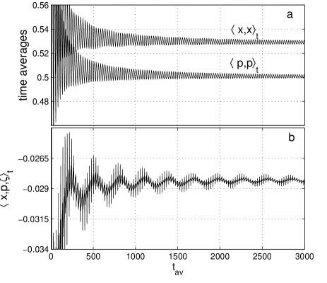
Figure 1: Dependence of the time averages $\langle x,x\rangle_{t}$, $\langle p,p\rangle_{t}$ (a) and $\langle x,p,\ \zeta\rangle_{t}$ (b) on $t_{av}$ for the NH thermostat in the regular regime of motion.

Special attention was payed to the properties of the cumulant $\kappa_{1,1,1}$ which in the numerical analysis is approximated by the time average $\langle x,p,\zeta\rangle_{t}$. In the previous subsection this variable was taken as a free parameter and it cannot be found from the equations. In the numerical approach it is obtained as the average over time along a trajectory and is always determined well. Numerical calculation shows that $\kappa_{1,1,1}$, as well as other cumulants connected with them (15, 16, 17), depends on the initial conditions. The dependence of $\langle x,p,\zeta\rangle_{t}\simeq\kappa_{1,1,1}$ on $x_{0}$ is shown in Fig.2 for $\zeta_{0}=0$, different $p_{0}$ and $t_{av}=3000$.

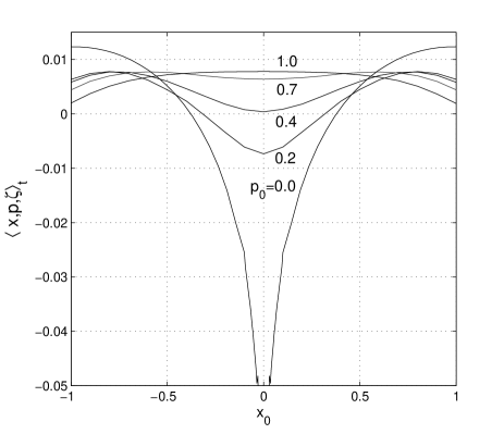
Figure 2: Dependence of the time average $\langle x,p,\zeta\rangle_{t}$ converging to $\kappa_{1,1,1}$ on the initial coordinate $x_{0}$ at different initial momenta $p_{0}$ and at the initial friction coefficient $\zeta_{0}=0$.

So, under the condition of the regular motion (motion on torus) the system PDF is non-canonical and it depends on the initial conditions, that is the PDF is different on different trajectories. This means that the system is not ergodic. This result is in quite agreement with the earlier obtained ones hoover ; legoll .

III.5 Chaotic motion

To study the chaotic regime of the system motion the values of the thermostat mass $\tau\leq 2$ and the initial values of the oscillator position $x_{0}=0$ and $0.5$, the momentum $p_{0}=4.0$, and $\zeta_{0}=0$ were chosen. The numerical analysis of the solutions of Eqs.(9) shows that the time averages corresponding to the canonical and non-canonical cumulants in this case behave differently.

The averages approximating to the canonical cumulants converge rapidly ($t_{av}\sim 10^{3}-10^{4}$) to corresponding solutions of the equations for cumulants. They are $\langle p,p\rangle_{t}$, converging to $\kappa_{0,2,0}$, and all averages converging to zero valued cumulants. As an example see the plot $\langle p,p\rangle_{t}$ vs $t_{av}$ in Fig.3.

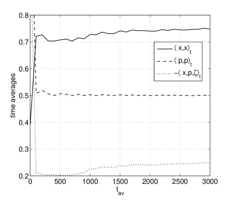
Figure 3: Dependence of the time averages $\langle x,x\rangle_{t}$, $\langle p,p\rangle_{t}$ and $\langle x,p,\ \zeta\rangle_{t}$ on $t_{av}$ for the NH thermostat in the chaotic regime of motion.

Other time averages approximating to the non-canonical cumulants converge to limiting values very slowly. The time average $\langle x,p,\zeta\rangle_{t}$ converging to $\kappa_{1,1,1}$ is shown in Fig.4 up to $t_{av}=10^{9}$ for different $\tau$ and initial conditions. It is clearly seen that the averaged values are still far from their limits.

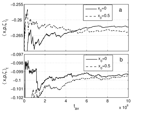
Figure 4: Dependence of the time averages $\langle x,p,\zeta\rangle_{t}$, on $t_{av}$ at the initial conditions $x_{0}=0$, $0.5$, $p_{0}=4$ and $\zeta_{0}=0$ for the NH thermostat at $\tau=2$ (a) and $\tau=0.1$ (b) in the chaotic regime of motion.

On the other hand all combinations of the time averages corresponding to the equations for cumulants, including Eqs.(15), converge to their zero values rather quickly ($t_{av}\sim 10^{3}-10^{4}$) in spite of the fact that some summands converge very slowly. An example of such behavior can be found in Fig.3 where the averages $\langle x,x\rangle_{t}$, $\langle p,p\rangle_{t}$ and $\langle x,p,\zeta\rangle_{t}$ are plotted as functions of $t_{av}$. It is seen that these averages at $t_{av}=3000$ satisfy the first equation in the set (15) with good accuracy while the individual terms are far from their stationary values.

In the previous section the dependence of the cumulant $\kappa_{1,1,1}$ on initial conditions was produced for the case of periodic motion. This became possible due to the rapid converging of the time averages. In the case of chaotic motion the situation is more difficult because of their slow converging. As it can be seen in Fig.4 that after averaging during time $t_{av}=10^{9}$ it is still impossible to conclude with certainty whether the limits corresponding to the initial conditions $x_{0}=0$ and $0.5$ coincide or differ. On the other hand at $\tau=2$ the system demonstrates chaotic motion under the initial conditions $x_{0}=0$, $p_{0}=4$, $\zeta=0$ and periodic one with $x_{0}=0$, $p_{0}=0.4$, $\zeta=0$ that is evidence of the nonergodicity of the system.

In the chaotic regime the dependence of the non-canonical cumulants (in particular $\kappa_{1,1,1}$) on the thermostat mass $\tau$ is of special interest. The dependence of $-\langle x,p,\zeta\rangle_{t}$ on $\tau$ is shown in Fig.5 with open circles in the double logarithmic scale. All points are obtained by the averaging over time and the accuracy of the obtained values is small. However the points corresponding to $\tau\leq 0.1$ demonstrate the linear dependence in the logarithmic scale. This corresponds to the power law which parameters were found by the mean square method

$$\kappa_{1,1,1}=-0.123\tau^{0.1}.$$ (20)

It is shown in Fig.5 by a solid line. Such behavior of the non-canonical cumulants means that the actual PDF, as $\tau$ decreases, approaches the canonical one.

This feature of the system statistical properties are connected with the existence of two characteristic times. The first one is the characteristic time of the mechanical motion of the oscillator in the phase space which is of the order of $t_{osc}\simeq 2\pi\sqrt{m/k}$. The second is the characteristic time of the energy exchange between the oscillator and thermostat and it is $t_{exch}=\sqrt{\tau}$. So, the conditions for obtaining good statistical properties of the thermostat is the inequality $t_{exch}\ll t_{osc}$.

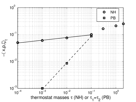
Figure 5: Dependence of the time averages $\langle x,p,\zeta\rangle_{t}$ on the thermostat mass for the NH and PB thermostats in the chaotic regime of motion.

IV Other thermostats

In this section the statistical properties of the harmonic oscillator coupled with more complicated thermostats are discussed. The phase spaces of these systems are four-dimensional. The extension of the dimension is due to the inclusion of an additional dynamical variable which is one more friction coefficient. The advantage of these thermostats is the fact that they ensure one more cumulant of the actual PDF to be canonical.

The statistical properties of the systems are similar to those discussed in the previous section. Therefore, they are discussed in less detail. Only the main traits and distinguishing features of the systems are represented. Besides, the statistical properties of the chaotic motion only are discussed.

IV.1 Patra-Bhattacharya thermostat.

The dynamical system, which is a harmonic oscillator coupled with the PB thermostat patra , can be described by the set of four ordinary differential equations

$$\dot{x} = \frac{p}{m}-\xi x,$$

$$\dot{p} = -kx-\zeta p,$$

$$\dot{\zeta} = \frac{1}{\tau_{1}}\left(\frac{p^{2}}{mT}-1\right),$$ (21)

$$\dot{\xi} = \frac{1}{\tau_{2}}\left(\frac{kx^{2}}{T}-1\right).$$

Here the phase variables $\textbf{q}=(x,p,\zeta,\xi)$ form a four-dimencional vector, $\xi$ is the additional configurational friction coefficient and $\tau_{1}$ and $\tau_{2}$ are the masses of the thermostats.

Gaussian PDF

$$W_{c}(\textbf{q})\propto\exp\left\{-\frac{p^{2}}{2mT}-\frac{kx^{2}}{2T}\right\}\exp\left\{-\frac{\zeta^{2}}{2\tau^{-1}_{1}}-\frac{\xi^{2}}{2\tau^{-1}_{2}}\right\}$$ (22)

obeys the stationary Liouville continuity equation corresponding to this system. The marginal PDF in the physical phase space $(x,p)$ is canonical and whole PDF is completely determined by four non-zero cumulants

$$\kappa_{2,0,0,0}=\frac{T}{k},\;\kappa_{0,2,0,0}=Tm,\;\kappa_{0,0,2,0}=\frac{1}{\tau_{1}},\;\kappa_{0,0,0,2}=\frac{1}{\tau_{2}}.$$ (23)

The kinetic coefficients of the system are

$$\textbf{K}_{1} = \left(K_{1x},K_{1p},K_{1\zeta},K_{1\xi}\right)=$$

$$= \left(\frac{p}{m}-\xi x,-kx-\zeta p,\frac{1}{\tau_{1}}\left(\frac{p^{2}}{mT}-1\right),\frac{1}{\tau_{2}}\left(\frac{kx^{2}}{T}-1\right)\right).$$

Only three equations for cumulants, demonstrating the main features of the actual PDF, are considered in this section. They are

$$\dot{\kappa}_{0,0,1,0} : \;\;\langle K_{1\zeta}\rangle=\frac{1}{\tau_{1}}\left(\frac{\langle p,p\rangle+\langle p\rangle^{2}}{mT}-1\right)=0,$$

$$\dot{\kappa}_{0,0,0,1} : \;\;\langle K_{1\xi}\rangle=\frac{1}{\tau_{2}}\left(\frac{k\langle x,x\rangle+k\langle x\rangle^{2}}{T}-1\right)=0,$$ (25)

$$\dot{\kappa}_{1,1,0,0} : \;\;\langle p,K_{1x}\rangle+\langle x,K_{1p}\rangle=$$

$$= \frac{1}{m}\langle p,p\rangle-\langle p,\xi x\rangle-k\langle x,x\rangle-\langle x,\zeta p\rangle=0.$$

In the first two equations the averages $\langle x^{2}\rangle$ and $\langle p^{2}\rangle$ are transformed in accordance with Eqs. (36) and (37). In order to get resulting expressions one need to open cumulant brackets $\langle x,\zeta p\rangle$ (38) and $\langle p,\xi x\rangle$ (39) and to take into account that all cumulants of the first order are equal to zero. The latter fact follows from the symmetry of Eqs. (21) and are verified by the numerical calculations.

As a result, Eqs. (25) lead to follow expressions for cumulants

$$\kappa_{0,2,0,0} = Tm,$$ (26)

$$\kappa_{2,0,0,0} = \frac{T}{k},$$ (27)

$$k\kappa_{2,0,0,0} = \frac{1}{m}\kappa_{0,2,0,0}-\kappa_{1,1,1,0}-\kappa_{1,1,0,1}.$$ (28)

The expressions (26) and (27) show that the cumulants $\kappa_{0,2,0,0}$ and $\kappa_{2,0,0,0}$ are canonical. This means that the PB thermostat controls both the kinetic and the configurational temperature in contrast to the NH thermostat which controls only the kinetic one.

The expression (28) together with (26) and (27) results in the equality $\kappa_{1,1,1,0}=-\kappa_{1,1,0,1}$. Numerical analysis shows that these cumulants are nonzero and the equality is satisfied well at $t_{av}\geq 1000$. This means that the PDF of the PB system is non-canonical because of the nonphysical statistical dependence of the phase variables.

It is clear from the structure of the equations (25) that non-canonical cumulants $\kappa_{1,1,1,0}$ and $\kappa_{1,1,0,1}$ in Eqs. (26)-(28) arise because of the presence of nonlinear terms $\zeta p$ and $\xi x$ in the equations of motion (21) that ensure the coupling of the oscillator with the thermostat. So, the origin of the non-canonicity of the PB system is the same as for the NH one, namely, the nonlinearity introduced into the equations of motion by the thermostat.

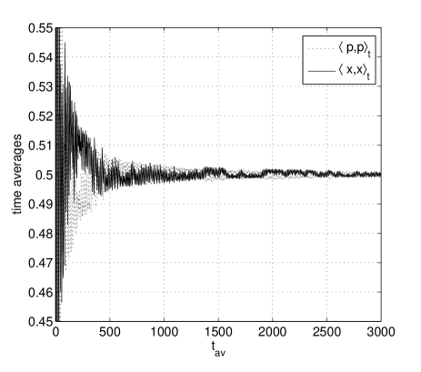
Figure 6: Dependence of the time averages $\langle x,x\rangle_{t}$, and $\langle p,p\rangle_{t}$ on $t_{av}$ for the PB thermostat at the initial conditions $x_{0}=0$, $p_{0}=4$, $\zeta_{0}=0$ and $\xi_{0}=0$.

The numerical solution of Eqs. (21), presented here, was obtained at the model parameters $k=m=1$, $T=0.5$, $\tau_{1}=\tau_{2}\leq 1$ and the initial conditions $x_{0}=0$ and $x_{0}=0.5$, $p_{0}=4$, $\zeta_{0}=0$ and $\xi_{0}=0$. The rates of converging of the time averages to the canonical and non-canonical cumulants, as well as in the case of the NH thermostat, vary greatly.

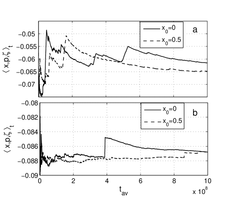
Figure 7: Dependence of the time averages $\langle x,p,\zeta\rangle_{t}$ on $t_{av}$ for the PB thermostat at the initial conditions $x_{0}=0$, $0.5$, $p_{0}=4$, $\zeta_{0}=0$ and $\xi_{0}=0$ and at $\tau_{1}=\tau_{2}=1$ (a) and $0.1$ (b).

The averages $\langle x,x\rangle_{t}$ and $\langle p,p\rangle_{t}$ approximating to the canonical cumulants $\kappa_{2,0,0,0}$ and $\kappa_{0,2,0,0}$ are shown in Fig.6 as functions of $t_{av}$. They converge rather rapidly to the configurational and kinethic temperatures $T=0.5$. On the other hand, the time average $\langle x,p,\zeta\rangle_{t}$ plotted in Fig.7 converges to $\kappa_{1,1,1,0}$ much slower.

The dependence of the $\langle x,p,\zeta\rangle_{t}\simeq\kappa_{1,1,1,0}$ on the thermostat masses $\tau_{1}=\tau_{2}$ is also established. It is shown in Fig.5 with open squares. The fitting function

$$\kappa_{1,1,1,0}=-0.837\tau^{0.99}$$ (29)

is plotted by a dashed line.

IV.2 Hoover-Holian thermostat.

The dynamical system which is a harmonic oscillator, coupled with the HH thermostat hh , can be represented by the set of four ordinary differential equations

$$\dot{x} = \frac{p}{m},$$

$$\dot{p} = -kx-\zeta p-\xi p^{3},$$

$$\dot{\zeta} = \frac{1}{\tau_{1}}\left(\frac{p^{2}}{mT}-1\right),$$ (30)

$$\dot{\xi} = \frac{1}{\tau_{2}}\left(\frac{p^{4}}{m^{2}T^{2}}-\frac{3p^{2}}{mT}\right).$$

The canonical Gaussian PDF (22) obeys the Liouville continuous equation corresponding to this system and it is completely defined by four nonzero cumulants (23).

The kinetic coefficients of the system are

$$\textbf{K}_{1} = \left(K_{1x},K_{1p},K_{1\zeta},K_{1\xi}\right)=$$

$$= \left(\frac{p}{m},-kx-\zeta p-\xi p^{3},\right.$$

$$\left.\;\;\;\frac{1}{\tau_{1}}\left(\frac{p^{2}}{mT}-1\right),\frac{1}{\tau_{2}}\left(\frac{p^{4}}{m^{2}T^{2}}-\frac{p^{2}}{mT}\right)\right).$$

The equations for cumulants, which are considered here, are

$$\dot{\kappa}_{0,0,1,0} : \;\;\langle K_{1\zeta}\rangle=\frac{1}{\tau_{1}}\left(\frac{\langle p,p\rangle+\langle p\rangle^{2}}{mT}-1\right)=0,$$

$$\dot{\kappa}_{0,0,0,1} : \;\;\langle K_{1\xi}\rangle=\frac{1}{\tau_{2}}\left(\frac{\langle p^{4}\rangle}{m^{2}T^{2}}-3\frac{\langle p^{2}\rangle}{mT}\right)=0,$$ (32)

$$\dot{\kappa}_{1,1,0,0} : \;\;\langle p,K_{1x}\rangle+\langle x,K_{1p}\rangle=$$

$$= \frac{1}{m}\langle p,p\rangle-k\langle x,x\rangle-\langle x,\zeta p\rangle-\langle x,\xi p^{3}\rangle=0.$$

After opening the cumulant brackets (see Appendix) and taking into account, that all cumulants of the first order and all joined cumulants of the second order are equal to zero (verified by numerical calculations), the solutions of the Eqs.(32) take the form

$$\kappa_{0,2,0,0} = mT,$$ (33)

$$\kappa_{0,4,0,0} = 3\kappa_{0,2,0,0}(mT-\kappa_{0,2,0,0})=0,$$ (34)

$$k\kappa_{2,0,0,0} = \kappa_{0,2,0,0}\left(\frac{1}{m}-3\kappa_{1,1,0,1}\right)-\kappa_{1,1,1,0}-\kappa_{1,3,0,1}.$$ (35)

Eq. (33) shows that the HH thermostat, as well as the NH and PB ones, controls the kinetic temperature of the system. The expression (34) demonstrates the fact that the HH thermostat controls additionally the fourth moment $\langle p^{4}\rangle$ (see Eq.(40)) in such a way as to ensure its equivalence to the canonical one. In the terms of cumulants this condition corresponds to the equality $\kappa_{0,4,0,0}=0$ (compare it with the same cumulant (18) of the NH system PDF).

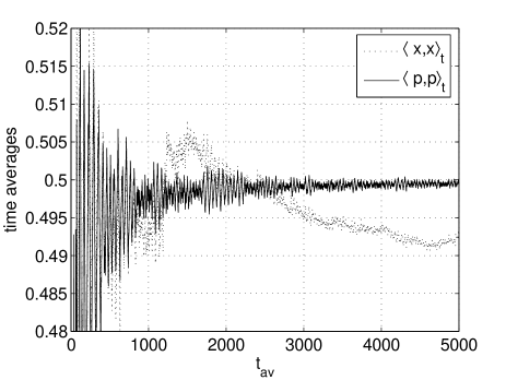
Figure 8: Dependence of the time averages $\langle x,x\rangle_{t}$ and $\langle p,p\rangle_{t}$ on $t_{av}$ for the HH thermostat at the initial conditions $x_{0}=0$, $p_{0}=4$, $\zeta_{0}=0$ and $\xi_{0}=0$.

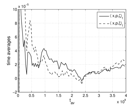
Figure 9: Dependence of the time averages $\langle x,p,\zeta\rangle_{t}$ and $\langle x,p,\xi\rangle_{t}$ on $t_{av}$ for the HH thermostat with masses $\tau_{1}=\tau_{2}=0.1$ at the initial conditions $x_{0}=0$, $p_{0}=4$, $\zeta_{0}=0$ and $\xi_{0}=0$.

The numerical analysis of the statistical properties of the dynamical system (30) shows that its behaviour is qualitatively similar to that of the NH and PB thermostats. The time averages approximating to the canonical cumulants converge rather rapidly to their equilibrium values (see $\langle p,p\rangle_{t}$ in Fig.8). But the averages approximating to the non-canonical cumulants converge much more slowly, Fig.9. The nonzero values of these cumulants, as it was shown in the previous cases, are the effect of the statistical dependence of the phase variables because of the nonlinearities $\zeta p$ and $\xi p^{4}$ introduced into the equations of motion by the thermostat.

V Discussion and conclusion

Equilibrium states in statistical mechanics are considered as canonical ensembles which are described by the Gibbs PDF. This PDF is determined by the total energy of the system. In most cases which are of interest the total energy is the sum of the kinetic and potential energies. Then the Gibbs PDF can be represented as a product of two functions, one of which depends only on momenta, and the other only on spatial coordinates. This means that the coordinates and momenta in the canonical ensemble are statistically independent.

The deterministic thermostats introduce additional nonlinearity into the equation of motion of the system. These nonlinearities lead to the appearance in the ensemble of nonphysical statistical dependencies between dynamical variables. In this work the analysis of these dependencies is represented on the example of three thermostats. The cumulant approach used is well suited for solving just this kind of problems.

The properties of the PDF of the harmonic oscillator, coupled with the NH, PB and HH thermostats, were analyzed. It is shown that the PDFs of the systems considered are non-canonical. This is revealed in the fact that some cumulants, which are equal to zero in the canonical PDF, are different from zero. This is a consequence of the statistical dependence of the phase variables because of the nonlinearities $\zeta p$, $\xi x$ and $\xi p^{3}$ introduced into the equations of motion by the thermostats. The degree of the non-canonicity of the PDFs studied can be evaluated by the value of the non-canonical cumulants, such as $\kappa_{1,1,1}$ for the NH thermostat or $\kappa_{1,1,1,0}$ and $\kappa_{1,1,0,1}$ for the PB and HH ones. For the NH and PB thermostats it is shown that the thermostat masses reduction leads to decreasing the values of non-canonical cumulants and, therefore, to approximating the actual PDF to the canonical one.

The ergodicity is more difficult to analyze. In the case of the quasiperiodic motion the situation is clear. The invariant tori exist in this case and the PDF of the system depends on the initial conditions because of such dependence of the non-canonical cumulants. This means that the system is nonergodic.

The chaotic regime of systems is more in line with the idea of ergodicity. But the cumulant method doesn’t allow to identify directly the ergodicity or nonergodicity of the system. It gives only sufficient conditions of ergodicity. If the set of equations for cumulants is well determinated, i.e. all equations are independent and the set is compatible, the system is ergodic. In this case the PDF is completely determined by the system parameters and doesn’t depend on the initial conditions for the equation of motion.

It should be noted that now it cannot be ruled out the possibility that these conditions are also necessary. But this statement has to be proved.

The systems that are analyzed in the work, do not meet these conditions. As it was shown in Sec.III, the set of equations for cumulants of the NH system splits into two subsets. One of the subsets is quite determinated and the other is underdetermined. The solutions of the first subset are the canonical cumulants and those of the second one are non-canonical. So, the whole set is underdetermined and the PDF of the system is non-canonical and, most likely, non-ergodic.

The PB and HH systems were studied in a lesser extent. But existence of the rapidly and slowly converging time averages to the canonical and non-canonical cumulants, analogous to that in the NH system, is indirect evidence in favour of the fact that the structure of the sets of the equations for cumulants are also analogous.

The existence of different rates of convergence of time averages, corresponding to canonical and noncanonical cumulants, also allows one to draw some conclusions about the ergodicity of the systems under discussion. To do this one have to take into account the difference in the behaviour of the regular and chaotic trajectories of the systems and the approximate nature of the numerical solution of the differential equations of motion of the systems.

A characteristic feature of periodic and quasiperiodic motions is that trajectories close at the initial time instant $t=0$ (close initial conditions) remain close for an arbitrarily long time. Chaotic trajectories behave differently. Trajectories that are arbitrary close at some point in time can diverge to a large distance (of the order of the characteristic system dimension) during a finite time approaching at the same time the trajectories with different initial conditions. This instability has been intensively studied using the Lyapunov exponent spectrum, see licht ; eckmann ; thompson and references therein.

A special feature of the numerical approach to the analysis of dynamical systems is that the differential equations of motion are replaced by difference equations with a finite time step $dt$. The solutions of such equations coincide with the differential ones only approximately. Their accuracy depends on the difference scheme used and the time step value. This means that the numerical solution at each time step jumps from one trajectory at time $t$ to another close one at time $t+dt$.

In the case of regular motion of the system the numerical trajectory occupies a small tube, thickness of which is determined by the method accuracy, around the exact trajectory. Since all exact trajectories that are placed in the tube correspond to close initial conditions, the averages calculated along the numerical one can be find with the required accuracy irrespective of their dependence on the initial conditions. An example of such calculations is shown in subsection III.4.

In the case of chaotic motion the situation is very different. A numerical trajectory in this case is not close to any exact one. It represents a set of points placed on different trajectories with very different boundary conditions. The averaging along such a trajectory is not the same as averaging along any exact one. If the value under calculation does not depend on the initial conditions, then it does not matter over which set of points the corresponding expression is averaged, the result will be achieved during rather short time and will be well determined. Canonical cumulants satisfy these conditions. Examples of the time averages converging to canonical cumulants can be seen in Figs.3, 6, 8. Otherwise, when the desired value depends on the initial conditions, the result of averaging along the numerical trajectory is not related to the time average along any exact trajectory. Under this condition the time averages of the corresponding expressions ”converge” much slower. This kind of behavior typical of non-canonical time averages can be seen in Figs.4, 7, 9. The behavior of the time averages described here is an indication that the PDFs of the NH, PB and HH thermostats depend on the initial conditions, and consequently the thermodynamic ensembles created by these thermostats are non-ergodic. Therefore, one can conclude that the canonicity and ergodicity of these systems are closely connected with each other, that is, the non-canonicity of the ensemble means its non-ergodicity.

Generalizing all the above-stated, one can conclude that not only the NH, PB and HH thermostats, but all deterministic thermostats create non-canonical and non-ergodic ensembles. The results obtained can also be qualitatively extended to nonlinear and many body systems. As it is shown above, non-physical correlations of dynamic variables, which are an attribute of an ensemble non-canonicity and, apparently, non-ergodicity, are determined by the presence of nonlinear terms in the equations of motion that provide a coupling of the system with the thermostat. The type of thermostat and its parameters affect only the degree of non-canonicity.

So, the cumulant approach is proposed as a new method for the studying the statistical properties of deterministically thermostated dynamical systems. In particular, it allows one to test the canonicity and ergodicity of the thermodynamical ensembles created by thermostats and to evaluate the degree of their non-canonicity. The applicability of the method is not limited only to the harmonic oscillator. It can be successfully used to investigate nonlinear and many-body systems. It is possible because there is no need to write out and analyze a large number of equations for cumulants to clarify the main statistical properties of the system. As it was shown by the example of the PB and HH thermostats, it is enough to study (numerically) only a small number of key cumulants.

*

Appendix A The expressions that are referenced in the text.

The opening of the cumulant brackets used in the text.

$$\langle x^{2}\rangle = \kappa_{2,0,0(,0)}+\kappa_{1,0,0(,0)}^{2},$$ (36)

$$\langle p^{2}\rangle = \kappa_{0,2,0(,0)}+\kappa_{0,1,0(,0)}^{2},$$ (37)

$$\langle x,\zeta p\rangle = \kappa_{1,1,1,0}+\kappa_{1,1,0,0}\kappa_{0,0,1,0}+\kappa_{1,0,1,0}\kappa_{0,1,0,0},$$ (38)

$$\langle p,\xi x\rangle = \kappa_{1,1,0,1}+\kappa_{0,1,0,1}\kappa_{1,0,0,0}+\kappa_{1,1,0,0}\kappa_{0,0,0,1},$$ (39)

$$\langle p^{4}\rangle = \kappa_{0,4,0,0}+3\kappa_{0,2,0,0}^{2}+4\kappa_{0,1,0,0}\kappa_{0,3,0,0}$$ (40)

$$+ 6\kappa_{0,1,0,0}^{2}\kappa_{0,2,0,0}+\kappa_{0,1,0,0}^{4},$$

$$\langle x,\xi p^{3}\rangle = \kappa_{1,3,0,1}+3\kappa_{1,2,0,1}\kappa_{0,1,0,0}+\kappa_{1,3,0,0}\kappa_{0,0,0,1}$$ (41)

$$+ 3\kappa_{1,1,0,1}\kappa_{0,1,0,0}^{2}+3\kappa_{1,2,0,0}\kappa_{0,1,0,0}\kappa_{0,0,0,1}$$

$$+ \kappa_{1,0,0,1}\kappa_{0,1,0,0}^{3}+3\kappa_{1,1,0,0}\kappa_{0,1,0,0}^{2}\kappa_{0,0,0,1}$$

$$+ 3\kappa_{1,0,0,1}\kappa_{0,2,0,0}\kappa_{0,1,0,0}+3\kappa_{1,1,0,0}\kappa_{0,1,0,1}\kappa_{0,1,0,0},$$

The example of the cumulants expressed in terms of the moments

$$\kappa_{0,2,0} = \langle p,p\rangle=\langle p^{2}\rangle-\langle p\rangle^{2},$$ (42)

$$\kappa_{1,1,1} = \langle x,p,\zeta\rangle=\langle xp\zeta\rangle-\langle x\rangle\langle p\zeta\rangle-\langle p\rangle\langle x\zeta\rangle$$ (43)

$$- \langle\zeta\rangle\langle xp\rangle+2\langle x\rangle\langle p\rangle\langle\zeta\rangle.$$

- (1) Nose S.: A unified formulation of the constant temperature molecular dynamics methods. J. Chem. Phys. 81, 511-519 (1984).
- (2) Hoover W.G.: Canonical dynamics: Equilibrium phase-space distributions. Phys. Rev. A 31, 1695-1697 (1985).
- (3) Patra P.K, Bhattacharya B.: A deterministic thermostat for controlling temperature using all degrees of freedom. J. Chem. Phys. 140, 064106 (2014)
- (4) Hoover W.G., Holian B.L.: Kinetic moments method for the canonical ensemble distribution. Phys. Lett. A 211, 253-257 (1996).
- (5) Kusnezov D., Bulgac A., and Bauer W.Kusnezov D.: Canonical Ensembles from Chaos. Ann. Phys. 204, 155-185 (1990).
- (6) Martyna G. J.,Klein M. L., and Tuckerman M.: Nose Hoover chains: The canonical ensemble via continuous dynamics. J. Chem. Phys. 97, 2635-2643 (1992).
- (7) Watanabe H. and Kobayashi H.: Ergodicity of a thermostat family of the Nose-Hoover type. Phys. Rev. E75, 040102(R) (2007).
- (8) Patra P.K., Bhattacharya B.: An ergodic configurational thermostat using selective control of higher order temperatures J. Chem. Phys. 142, 194103-1-8 (2015).
- (9) Samoletov A., and Vasiev V.: Dynamic principle for ensemble control tools. J. Chem. Phys. 147, 204106 (2017).
- (10) Posch H. A., Hoover W. G.,Vesely F. J.: Canonical dynamics of the Nose oscillator: Stability, order, and chaos. Phys. Rev.A 33, 4253-4265 (1986).
- (11) Legoll F., Luskin M., and Moeckel R.: Non-Ergodicity of the Nose Hoover Thermostatted Harmonic Oscillator. Arch. Ration. Mech. Anal. 184, 449-463 (2007).
- (12) Patra P.K., Bhattacharya B.: Nonergodicity of the Nose-Hoover chain thermostat in computationally achievable time. Phys. Rev. E 90, 043304 (2014).
- (13) Hoover W.G., Hoover C. G.: Ergodicity of a Time-Reversibly Thermostated Harmonic Oscillator and the 2014 Ian Snook Prize. CMST 20, 87-92 (2014).
- (14) Hoover W.G., Hoover C. G., Isbister D. J.: Chaos, ergodic convergence, and fractal instability for a thermostated canonical harmonic oscillator. Phys. Rev. E 63, 026209-1-5 (2001).
- (15) Patra P.K., Sprott J. C., Hoover W.G., Hoover C. G.: Deterministic time-reversible thermostats: chaos, ergodicity, and the zeroth law of thermodynamics. Mol. Phys. 113, 2863-2872 (2015).
- (16) Hoover W.G., Hoover C. G.: Ergodicity of the Martyna-Klein-Tuckerman Thermostat and the 2014 Ian Snook Prize. CMST 21, 5-10 (2015).
- (17) Hoover W.G., Sprott J. C., Patra P.K.: Ergodic time-reversible chaos for Gibbs canonical oscillator. Phys. Lett. A 379, 2935-2940 (2015).
- (18) Samoletov A. A., Dettman C. P., Chaplain C. P.: Thermostats for ”slow” configurational modes. J. Stat. Phys. 128, 1321-1336 (2007).
- (19) Malakhov A. N.: Cumulant Analysis of Random Non-Gaussian Processes and their Transformation. Sovetskoe Radio, Moscow (1978) (in Russian).
- (20) Primak S., Kontorovich V.,Lyandres V.: Stochastic Methods and their Applications to Communications. Stochastic Differential Equations Approach. Wiley, New York (2004).
- (21) Kontorovich V.: Applied statistical analysis for strange attractors and related problems. Math. Meth. Appl. Sci., 30, 1705-1717 (2007)
- (22) Hockney R. W.: The potential calculation and some applications. Methods Comput. Phys. 9, 136-211 (1970).
- (23) Verlet L.: Computer ”experiment” on classical fluids. 1. Thermodynamical properties of Lennard-Jones molecules. Phys. Rev. 159, 98-103 (1967).
- (24) Lichtenberg A. J., Liberman M. A.: Regular and Stochastic Motion. Springer-Verlag, New York (1983).
- (25) Eckmann J.-P., Ruelle D.: Ergodic Theory of Chaos and Strange Attractors. Rev. Mod. Phys. 57 (1985).
- (26) Thompson J. M. T. Stewar, H. B.: Nonlinear Dynamics and Chaos Wiley, New York, 1986.